A First Look at BISTRO Observations of The $\rho$ Oph-A core

Abstract

We present 850 $\mu$m imaging polarimetry data of the $\rho$ Oph-A core taken with the Submillimeter Common-User Bolometer Array-2 (SCUBA-2) and its polarimeter (POL-2), as part of our ongoing survey project, BISTRO ($\bm{B}$-fields In STar forming RegiOns). The polarization vectors are used to identify the orientation of the magnetic field projected on the plane of the sky at a resolution of 0.01 pc. We identify 10 subregions with distinct polarization fractions and angles in the 0.2 pc $\rho$ Oph A core; some of them can be part of a coherent magnetic field structure in the $\rho$ Oph region. The results are consistent with previous observations of the brightest regions of $\rho$ Oph-A, where the degrees of polarization are at a level of a few percents, but our data reveal for the first time the magnetic field structures in the fainter regions surrounding the core where the degree of polarization is much higher ($>5\%$). A comparison with previous near-infrared polarimetric data shows that there are several magnetic field components which are consistent at near-infrared and submillimeter wavelengths. Using the Davis-Chandrasekhar-Fermi method, we also derive magnetic field strengths in several sub-core regions, which range from approximately 0.2 to 5 mG. We also find a correlation between the magnetic field orientations projected on the sky with the core centroid velocity components.

=130

1 INTRODUCTION

Stars form in dense and cold molecular clouds and it has long been considered that magnetic fields may play significant roles in various stages of star formation (e.g., Shu et al., 1987; Bergin & Tafalla, 2007; McKee & Ostriker, 2007; André et al., 2013). Near-infrared linear polarimetry is one of the traditional methods of tracing magnetic field structure in order to measure the magnetic fields in denser regions than those traced by optical polarimetry, which are directly related to the star formation process (e.g., Davis & Greenstein, 1951; Lazarian, 2007). The magnetic field has been successfully traced in dense regions of several molecular clouds (e.g., Wilking et al., 1979; Tamura et al., 1987, 1988, 2007; Kwon et al., 2010, 2011, 2015; Cashman & Clemens, 2014; Santos et al., 2014; Ward-Thompson et al., 2017a). Polarization at near-infrared wavelengths, however, relies on measurements of dust extinction from background stars and as such cannot trace well magnetic fields in denser substructures like filaments and cores within clouds. As these structures are directly linked to star formation, it is vital to measure their magnetic fields. Observations of dust polarization from thermal emission at far-infrared and (sub)millimeter wavelengths can trace these high column densities and probe how the magnetic field influences the star formation process (e.g., Tamura et al., 1999; Pattle et al., 2015; Ward-Thompson et al., 2017b; see also Soler et al. 2016).

The $\rho$ Ophiuchi (hereafter $\rho$ Oph) dark cloud complex is one of the closest star-forming regions at a distance of approximately 120–165 pc (e.g., Chini, 1981; de Geus et al., 1989; Knude & Hog, 1998; Rebull et al., 2004; Loinard et al., 2008; Lombardi et al., 2008; Mamajek, 2008; Snow et al., 2008; Ortiz-León et al., 2017). It has also been widely studied (see Kwon et al., 2015; Wilking et al., 2008, for a reference summary). It is a nearby region of clustered low- to intermediate-mass star formation (e.g., Wilking et al., 2008) and is heavily influenced by the nearby Sco OB2 association (Vrba, 1977; Loren, 1989a, b; Kwon et al., 2015). It was observed as part of the JCMT Gould Belt Legacy Survey (Ward-Thompson et al., 2007), the Herschel Gould Belt Survey (André et al., 2010), and the Spitzer Gould Belt Survey (Evans et al., 2009). In the main body of $\rho$ Oph, detailed DCO⁺ observations have identified several very dense, cold cores labeled A–F (Loren & Wootten, 1986; Loren et al., 1990), and $\rho$ Oph-A appears to be the warmest among these cores (Zeng et al., 1984). The first submillimeter continuum observations of the $\rho$ Oph-A core region were obtained by Ward-Thompson et al. (1989). Many sub-cores in this region were identified (e.g., André et al. 2007; Motte et al. 1998), which will be described in Section 5. In this paper, we use the term “core” for the $\rho$ Oph-A complex and the term “sub-core” for the smaller condensations within it.

Here we present new observations of the $\rho$ Oph-A core in dust polarization from the James Clerk Maxwell Telescope (JCMT) as part of the $\bm{B}$-fields In STar forming RegiOns (BISTRO) survey (Ward-Thompson et al., 2017a). The JCMT magnetic field survey of the Gould Belt clouds is a large-scale project, which aims to map the submillimeter polarization of the dust thermal emission in the densest parts of all of the Gould Belt star forming regions. The combination of SCUBA-2 (Submillimeter Common-User Bolometer Array-2; Holland et al., 2013) and its polarimeter POL-2 (Bastien et al, in prep.) enables deep submillimeter polarimetry and is one of the most powerful instruments to reveal the magnetic field structure in star forming regions thanks to its high sensitivity and high resolution (Ward-Thompson et al. 2017a; Pattle et al. 2017).

The paper is outlined as follows: In Section 2, we describe the submillimeter observations, and the SCUBA-2/POL-2 data reduction is described in Section 3. In Section 4, we present the results of the submillimeter imaging polarimetry. In Section 5, we discuss the magnetic field structure related to the star-forming activity in the $\rho$ Oph-A core region. A summary is given in Section 6.

2 OBSERVATIONS

Continuum observations of $\rho$ Oph-A at 850 $\mu$m were made by inserting POL-2 into the optical path of SCUBA-2 between 2016 April 15 and 2016 April 24. The region was observed in 20 sets of 41-minute observations and among the 20 sets, 2 sets with bad quality data were excluded. Note that the BISTRO time was allocated to take place during Band 2 weather ($0.05<\tau_{225\rm\,GHz}<0.08$). The observations were made using fully-sampled 12$\arcmin$ diameter circular regions with a resolution of 14$\farcs$1 using a version of the SCUBA-2 DAISY mapping mode (Holland et al., 2013) optimized for POL-2 observations. The POL-2 DAISY scan pattern produces a central 3$\arcmin$ diameter region of approximately even coverage, with noise increasing to the edge of the map. The mode has a scan speed of 8$\arcsec$/s, with a half-waveplate rotation speed of 2 Hz (Friberg et al., 2016). Continuum polarimetric observations were simultaneously taken at 450 $\mu$m with a resolution of 9.6$\arcsec$. In this paper we discuss 850 $\mu$m data only.

3 DATA REDUCTION

The 850 $\mu$m POL-2 data were reduced in a three-stage process using the $pol2map$ routine (the version updated on 2017 May 27) in smurf (Berry et al. 2005; Chapin et al. 2013), which we summarize here. POL-2 data reduction is described in detail by Bastien et al. (in prep.). See also Ward-Thompson et al. 2017a for a brief summary.

In the first stage, the raw bolometer timestreams for each observation are converted into separate Stokes $Q$, $U$, and $I$ timestreams using the process $calcqu$. An initial Stokes $I$ map is created from the $I$ timestream from each observation using the iterative map-making routine $makemap$. For each reduction, areas of astrophysical emission are defined using a signal-to-noise-based mask determined iteratively by $makemap$. Areas outside this masked region are set to zero until the final iteration of $makemap$ (see Mairs et al. 2015 for a detailed description of the role of masking in SCUBA-2 data reduction). Each map is compared to the first map in the sequence to determine a set of relative pointing corrections. The individual $I$ maps are coadded to produce an initial $I$ map of the region.

In the second stage, an improved Stokes $I$ map is created from the $I$ timestreams of each observation using $makemap$. The initial $I$ map (described above) is used to generate a fixed signal-to-noise-based mask for all iterations of $makemap$. The pointing corrections determined in Stage 1 are applied during the map-making process. In all cases, the polarized sky background is estimated by doing a Principal Component Analysis (PCA) of the $I$, $Q$, and $U$ timestreams to identify components that are common to multiple bolometers. In the first stage, the 50 most correlated components are removed at each iteration. In the second stage 150 components are removed at each iteration, resulting in smaller changes in the map between iterations and lower noise in the final map. All of the individual improved $I$ maps are co-added to form the final output $I$ map.

In the third stage, the Stokes $Q$ and $U$ maps, and the final vector catalogue, are created. Individual $Q$ and $U$ maps are reduced separately using $makemap$, and are created from the timestreams created in Stage 1, using the same mask based on the initial Stokes $I$ map as was used in Stage 2, and using the pointing offsets determined in Stage 1. Correction for instrumental polarization is performed, based on the final output $I$ map. The sets of individual $Q$ and $U$ maps are then coadded to create final $Q$ and $U$ maps. The final coadded Stokes $Q$, $U$ and $I$ maps are used to create an output vector catalogue, which includes the coordinates (J2000.0), values of Stokes parameters, degrees of polarization ($P\pm\delta P$), and polarization position angles ($\theta\pm\delta\theta$). Therefore, it uses exactly the same map-making procedure to create all three maps – Stokes $Q$, $U$, and $I$, and spatial frequencies present in the three maps are all in common.

The output $Q$, $U$ and $I$ maps are gridded to 4^′′ pixels and are calibrated in mJy beam^-1 using a flux conversion factor (FCF) of 725 Jy pW^-1 (the standard SCUBA-2 850 $\mu$m FCF of 537 Jy pW^-1 multiplied by a factor of 1.35 to account for additional losses from POL-2; cf. Dempsey et al. 2013; Friberg et al. 2016). The output vectors are debiased using the mean of their $Q$ and $U$ variances to remove statistical biasing in regions of low signal-to-noise (see Equation 3 below).

The raw degree of polarization, $P^{\prime}$, and the uncertainty in the degree of polarization, $\delta P$, can be calculated from the expressions:

$$P^{\prime}={\sqrt{Q^{2}+U^{2}}\over I}\times 100\%$$ (1)

and

$$\delta P^{\prime}=(P^{\prime}I^{2})^{-1}\sqrt{(Q^{2}\delta Q^{2}+U^{2}\delta U^{2}+(P^{\prime})^{4}I^{2}\delta I^{2})}$$ (2)

Note that in the pipeline software (without debiasing; see below), $P^{\prime}I$ is first calculated from $Q$, $\delta Q$, $U$, and $\delta U$, then $\delta P^{\prime}$ is calculated from $I$, $\delta I$, $Q$, $U$, and $\delta PI$. The expression here is identical to the formula in the pipeline but tries to show the dependence on the errors of $I$, $Q$, and $U$.

As mentioned, a bias exists that tends to increase the polarization percentage value, even when Stokes $Q$ and $U$ are consistent with a value of zero because polarization percentage is forced to be positive (Vaillancourt, 2006). To mitigate this problem, approximate de-biased values are calculated in the pipeline, assuming $\delta Q\sim\delta U$, as follows:

$$PI=\sqrt{Q^{2}+U^{2}-0.5(\delta Q^{2}+\delta U^{2})}$$ (3)

and the degree of polarization $P$ is derived from the polarized intensity $PI$ as

$$P=PI/I.$$ (4)

The polarization position angles, $\theta$, and their errors, $\delta\theta$, can then be calculated by the following relations:

$$\theta={1\over 2}\,{\rm tan}^{-1}{U\over Q}$$ (5)

and

$$\delta\theta=0.5\times\sqrt{Q^{2}\times\delta U^{2}+U^{2}\times\delta Q^{2}}/(Q^{2}+U^{2})\times 180\arcdeg/\pi$$ (6)

The data reduction process described above derives the Stokes $I$ map from the same POL-2 observations that are used to derive the Stokes $Q$ and $U$ maps. A consequence of this is that the FCF for the Stokes $I$, $Q$, and $U$ maps are then all equal and so cancel out when calculating the fractional polarization. As a result, the $I$ and the $Q$ and $U$ maps necessarily have exactly the same spatial scales. Earlier versions of the POL-2 pipeline software derived the Stokes $I$ map from separate observations taken without POL-2 in the beam, resulting in the $I$ map having a different FCF to the Stokes $Q$ and $U$ maps because of the attenuation caused by POL-2 and differences in the map-making procedure (cf. Friberg et al. 2016).

4 Results

4.1 POL-2 Data Verification

The BISTRO survey has recently begun to systematically investigate magnetic field structures in the dense cores using measurements of polarized dust emission, which is one of the most effective ways of probing the magnetic fields of such cores. Since POL-2 is newly commissioned, it is an important step to verify the consistency of our new data with those of previous studies. Therefore, we compare the POL-2 observations of $\rho$ Oph-A with data from the SCUPOL polarimeter on the previous generation submillimeter bolometer array on the JCMT, SCUBA (Greaves et al., 1999).

Figure 1 shows the 850 $\mu$m intensity map (Stokes $I$) obtained using the JCMT with SCUBA-2/POL-2 with well known submillimeter and infrared sources labeled. The Stokes $I$ image is consistent with previous deep submillimeter continuum images (e.g., Pattle et al. 2015).

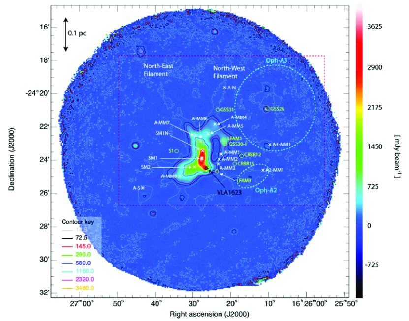
Figure 1: Stokes $I$ image (linear scale) of the $\rho$ Oph-A field centered on Oph-A1 (Motte et al., 1998) obtained using JCMT with SCUBA-2/POL-2. Notable sources and features in this region are labeled. The spatial resolution is 14$\farcs$1 or approximately 0.01 pc assuming a distance to the Oph cloud of 140 pc. The white crosses indicate the positions of the starless condensations identified by Motte et al. (1998) in the dust continuum at 1.2 mm (corresponding to the red dashed rectangle region in this figure), the yellow circles indicate the position of young embedded stars, and the black star indicates the position of VLA 1623. The cyan dashed circles indicate Oph-A2 and Oph-A3, respectively, defined by Motte et al. (1998). The contour levels are arbitrarily chosen to emphasize the Oph-A core and their keys are shown in mJy beam^-1 unit.

Figure 2 shows a comparison between the SCUBA-2/POL-2 data and the previous polarization data from SCUPOL (Greaves et al., 1999). Figures 2(a)–(c) respectively show Stokes $I$, $Q$, and $U$ images of the $\rho$ Oph-A core region obtained from the JCMT with SCUBA-2/POL-2 (this work), and Figures 2(d)–(f) respectively show Stokes $I$, $Q$, and $U$ images of the $\rho$ Oph-A core region obtained from JCMT with SCUPOL (previous work; see also the SCUBA Polarimeter Legacy Catalogue, Matthews et al. 2009). The black boxes in Figures 2(a)–(c) show the regions covered by SCUPOL. As shown in Figure 2, our data are deeper and more clearly provide the morphology of the surrounding regions in all of the Stokes $I$, $Q$, and $U$ images, although two have the same spatial resolution. However, it should be noted that the SCUPOL data are binned to generate 10$\arcsec$ polarization vectors.

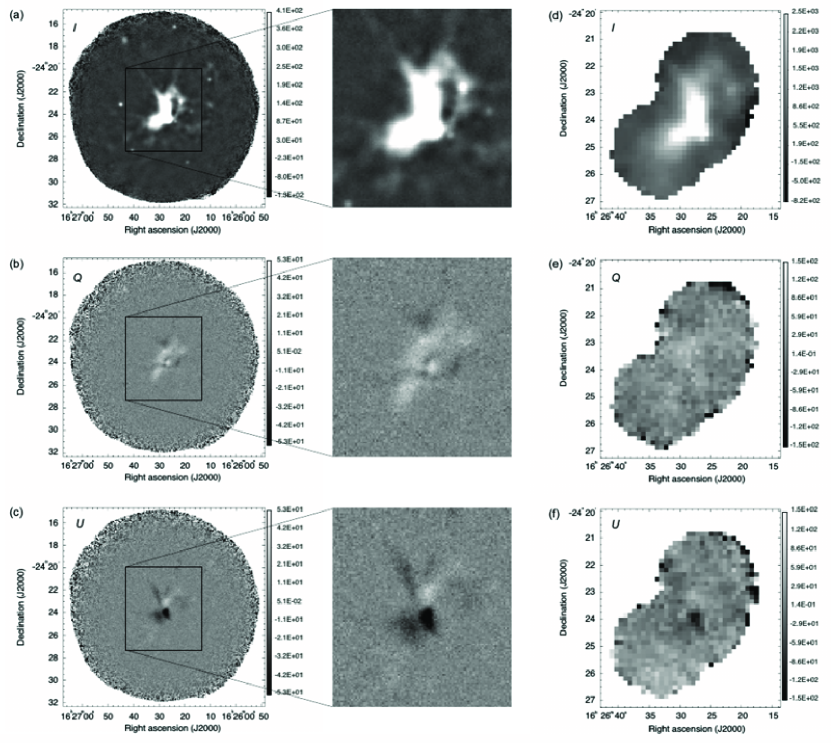
Figure 2: SCUBA-2/POL-2 data (this work) compared with SCUPOL (previous work). The intensity grey scales are different between the POL-2 and SCUPOL data. (a)–(c) Stokes $I$, $Q$, and $U$ images (linear scale) of the $\rho$ Oph-A core region obtained with the JCMT with SCUBA-2/POL-2. The Stokes $Q$ and $U$ images (b and c) have the same grey scale in mJy beam^-1 units. The SCUPOL field of view (d)–(f) is indicated by a black box in Figures 2(a)–(c), respectively. (d)–(f) 850 $\mu$m Stokes $I$, $Q$, and $U$ images of the $\rho$ Oph-A core region obtained from the JCMT with SCUPOL (from The SCUBA Polarimeter Legacy Catalogue). The Stokes $Q$ and $U$ images (e and f) have the same grey scale in mJy beam^-1 units. The original units are pW and Volt in the SCUBA-2/POL-2 and SCUPOL data, which are converted to mJy using the conversion factors of 725 Jy beam^-1 pW^-1 and 455 Jy beam^-1 Volt^-1 (see Matthews et al. 2009). Note that the SCUPOL data are binned to generate 10$\arcsec$ vectors. The grey scale ranges in SCUBA-2/POL-2 and SCUPOL are different so that fainter regions in $Q$ and $U$ images are clearly seen in each image.

To compare the best intensity morphology with that from the previous data, we first introduce the detailed submillimeter morphology of the $\rho$ Oph-A core, and then present the polarimetric results.

4.2 Morphology of $\rho$ Oph-A

Figure 1 shows the morphology of $\rho$ Oph-A from our 850 $\mu$m Stokes $I$ emission map. The region contains several sub-cores, which we outline below:

Oph-A SM1

Oph-A SM1 is a sub-core located toward the peak of the 850 $\mu$m intensity (Ward-Thompson et al. 1989, also cf. Figure 1). It has the brightest submillimeter continuum in all of $\rho$ Oph. The filamentary morphology in $\rho$ Oph suggests that SM1 may be influenced by the B4 star Oph S1 (cf. Figure 1), which is a nearby young B-type star. Motte et al. (1998) report that the total mass and dust temperature of Oph-A SM1 are 2 $M_{\sun}$ and $T\approx 20$ K, respectively.

VLA 1623

VLA 1623 is the prototypical Class 0 star (André et al., 1993). It drives a large-scale bipolar molecular outflow (Dent et al., 1995; Yu & Chernin, 1997) and is embedded within a nearly spherical dust envelope (André et al., 1993). Bontemps & Andre (1997) found three emission clumps at centimeter wavelengths with the Very Large Array, which they interpreted as knots in the radio jet driving the large CO outflow (see also, Chen et al. 2013). However, the position angles of the radio jet and the CO outflow differ by approximately 30°. Clump A was further resolved into two components at a high angular resolution (Chen et al., 2013), with the Submillimeter Array (SMA). VLA 1623 is also binary system, with two components separated at high angular resolutions (Looney et al., 2000; Ward-Thompson et al., 2011). Since the POL-2 resolution is approximately 14$\farcs$1 at 850 $\mu$m, we cannot separate these components and refer to them as a single source, VLA 1623 in this paper.

Other local structures

There are two filaments in the north part of the $\rho$ Oph-A core. These structures are consistent with not only the results obtained with SCUBA on the JCMT (Wilson et al., 1999) but also those seen in the map made with SCUBA-2 (Pattle et al., 2015) and IRAM (Motte et al., 1998) results. In addition to the filaments, Wilson et al. (1999) reported that there are two arcs of emission in the direction of the northwest extension of the VLA 1623 outflow. The outer arc appears relatively smooth at 850 $\mu$m, while the inner arc breaks up into a number of individual clumps, some of which are known protostars.

4.3 New Submillimeter Polarization Vector Map

Polarized thermal emission from dust grains in clouds offers an ideal probe of the magnetic field structure on multiple scales, from protostellar disks to cores and clumps (e.g., Matthews et al., 2001; Crutcher et al., 2004).

Figure 3 shows our submillimeter polarization vector maps of the $\rho$ Oph-A region, observed with SCUBA-2/POL-2. Since it is worthwhile to directly compare our data with the previous submillimeter polarization vector map, Figure 3 is prepared with the same criteria, $I>0$, $P/\delta P>2$, and $\delta P<4\%$, as were used in the previous results by SCUPOL (See Figure 44 of Matthews et al. 2009). The selection criteria here are mainly for the purpose of the comparison with the SCUPOL data; however, we have found this to be fairly reasonable to see the magnetic field structure in this region by changing various $P/\delta P$ or $\delta P$ selections. In addition, Figure 3 suggests the vector maps with both $P/\delta P>2$ and $P/\delta P>3$ are almost the same, if we use the additional criterion of $\delta P<4\%$. Without this $\delta P$ criterion, the vector map with $P/\delta P>2$ has many more vectors, but has RMS noise values of $\delta P$ and $\delta\theta$ too high to allow interpretation of the magnetic field behavior. Therefore, we use the criteria of $I>0$, $P/\delta P>2$, and $\delta P<4\%$ in the following discussion to maximize the number of polarization vectors that can be used for our discussion below on the magnetic field directions. The angle errors ($\delta\theta$) of approximately 15$\arcdeg$ in the 2$\sigma$ case are acceptable for such discussions. Therefore, we show both 2$\sigma$ and 3$\sigma$ cases in several figures and use 2$\sigma$ data for the discussion on magnetic field directions.

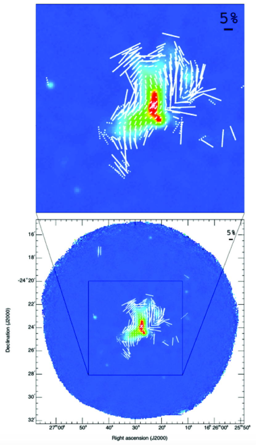
Figure 3: The 850 $\mu$m polarization vector maps. The vectors are sampled on a 12$\arcsec$ grid ($3\times 3$ pixel smoothing) and plotted where $I>0$, $P/\delta P>2$, and $\delta P<4\%$ (dotted vectors) and $I>0$, $P/\delta P>3$, and $\delta P<4\%$ (solid vectors), respectively.

Our data are more sensitive than those obtained by SCUPOL as shown in Section 4.1. The new submillimeter polarization vectors inside the dense regions agree well with the results by Matthews et al. (2009), especially in the bright region near SM1. The dominant submillimeter polarization position angle in the bright region is approximately 130$\arcdeg$ (as discussed in the following section). We have also checked if our new data are consistent with the JCMT 800 $\mu$m aperture polarimetric data of Holland et al. (1996). The measured positions are not exactly the same, but both $P$ and $\theta$ values are consistent with each other between the two studies.

Note that there are clear inconsistencies between SCUBA-2/POL-2 and SCUPOL data in the outer parts of the Oph-A core region. To the south-east and south of the core, SCUPOL data show more numerous polarization vectors even at a very low intensity level while to the north-west and north-east, SCUBA-2/POL-2 data reveal more vectors. Since our data have a higher S/N ratio, as shown in Figure 2, we believe that our SCUBA-2/POL-2 data are more reliable in the faint outer regions, down to approximately 30 mJy beam^-1, while care is necessary when using the SCUPOL vectors in the outer regions. The reason why the SCUPOL data have more vectors in some outer core regions is not clear. However, we note that the SCUPOL maps were made by chopping, while POL-2 in a scanning mode. Therefore, the chopping effect cannot be excluded in the SCUPOL data, which were taken at different times by different observers.

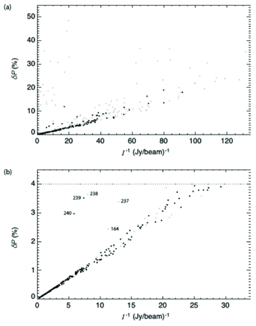
Figure 4: Degree of polarization errors ($\delta P$) vs. 1/Intensity ($I$). Five dots with large $\delta P$ are labeled (cf. Table 1). These five sources are located in outer regions of the Oph-A core region where the noise levels are higher. (a) Grey circles: $I>0$, $P/\delta P>2$. Black circles: $I>0$, $P/\delta P>3$. (b) Grey circles: $I>0$, $P/\delta P>2$, and $\delta P<4\%$. Black circles: $I>0$, $P/\delta P>3$, and $\delta P<4\%$.

Based on the robustness toward the fainter regions mentioned above, our data clearly show the polarizations in the fainter regions surrounding the core and the degrees of polarization are much higher ($>5\%$) in the outer envelope. This trend is clear in our polarization map whose vector length is proportional to the degree of polarization (see also Figure 7).

4.4 Experimental Criteria

Figure 4 shows the degree of polarization errors ($\delta P$) versus the inverse intensity ($I^{-1}$); the polarization uncertainty increases steadily with decreasing intensity. For $\delta P>4\%$, we see significant scatter in this relation, whereas the data with $\delta P<4\%$ are fairly well correlated. There are five vectors with $\delta P<4\%$ that show substantial scatter from the main trend and are labeled on Figure 4 (cf. Table 1). Aside from these five cases, vectors with $\delta P<4\%$ appear to be robust. All five anomalous positions (ID: 164, 237, 238, 239, 240) are located near the map boundary where the noise levels are higher. Vector 164 is located in the east of Oph-A, and vector 237 is located between the north-west filamentary structure and GSS 26 and vectors, 238, 239 and 240, are located in the upper part of the north-east filamentary structure. Note that including these five vectors does not affect our results. Figure 4 also shows that our polarization data present a large scatter when the intensity levels are less than approximately 30 mJy beam^-1, which corresponds to $N$(H₂) $\sim$ 4 $\times$ 10²¹ cm^-2 assuming a temperature of 10 K (Kauffmann, 2007).

5 DISCUSSION

Magnetic fields in star formation are significant as they can influence core collapse, star formation rates, and molecular cloud lifetimes (e.g., Myers & Goodman, 1988; Hartmann et al., 2001; Elmegreen, 2000). We use our polarization data to determine the magnetic field strength in $\rho$ Oph-A below.

5.1 Magnetic Field Structures in $\rho$ Oph-A

The $\rho$ Oph molecular cloud has been observed with 1.3 mm continuum mapping (Motte et al., 1998) and line mapping (Umemoto et al. 1999, see also White et al. 2015), and the $\rho$ Oph-A core region is one of the most obvious sources. Matthews et al. (2009) presented a bulk analysis of SCUPOL 850 $\mu$m polarization vector maps, which include the $\rho$ Oph-A core. The submillimeter polarization position angle is about 130$\arcdeg$ in average (measured east of north), which indicates a magnetic field direction of approximately 40$\arcdeg$ (by rotating the submillimeter polarization vectors by 90$\arcdeg$). This angle is consistent with the well-known 50$\arcdeg$ component determined via infrared polarimetry observations (Sato et al., 1988; Kwon et al., 2015). Therefore, the magnetic field seems largely consistent between the outer low-density cloud and the high density cores.

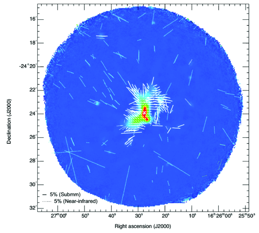
Figure 5: Same as Figure 3 but rotated by 90$\arcdeg$ with near-infrared polarization vectors (cyan dotted vectors) from Kwon et al. (2015). These vectors therefore show the inferred magnetic field orientation projected on the plane of the sky. Scale vectors of 5% at submillimeter and near-infrared wavelengths are shown in the bottom left corner.

To investigate magnetic field structures in this region in more detail, we use the POL-2 polarization vectors rotated by 90$\arcdeg$, as shown in Figure 5. Figure 6 shows the inferred morphology of the magnetic field in the $\rho$ Oph-A core region. In this figure, vector maps are shown in two ways; one selected with the polarization signal-to-noise ratio ($P/\delta P>$ 2 or 3) and the other selected with the intensity signal-to-noise ratio ($I/\delta I>20$). The latter intensity-selection is shown because selecting by S/N in $P$ will tend to bias the polarization data sample to high $P$ values (especially towards regions of low intensity), so a comparison with a sample selected by $I/\delta I$ is made to show that without this bias the polarization fraction is still larger on average for cloud sightlines in the envelope. Figure 7 demonstrates that this correlation is robust, as seen also from the negative correlation between the degrees of polarization and intensities in both of the $P$ and $I$ selection data. We find that $P\propto I^{\gamma}$ where $\gamma\sim-0.8$ for the $P$ selection to $-0.7$ for the $I$ selection. Note that there is a larger dispersion at the low-intensity regions in the $I$ selection because not only high $P$ data but also several low $P$ data exist in the $I$ selection. This trend might be due to a combination of several factors such grain alignment and magnetic field geometry. A detailed discussion will be presented elsewhere.

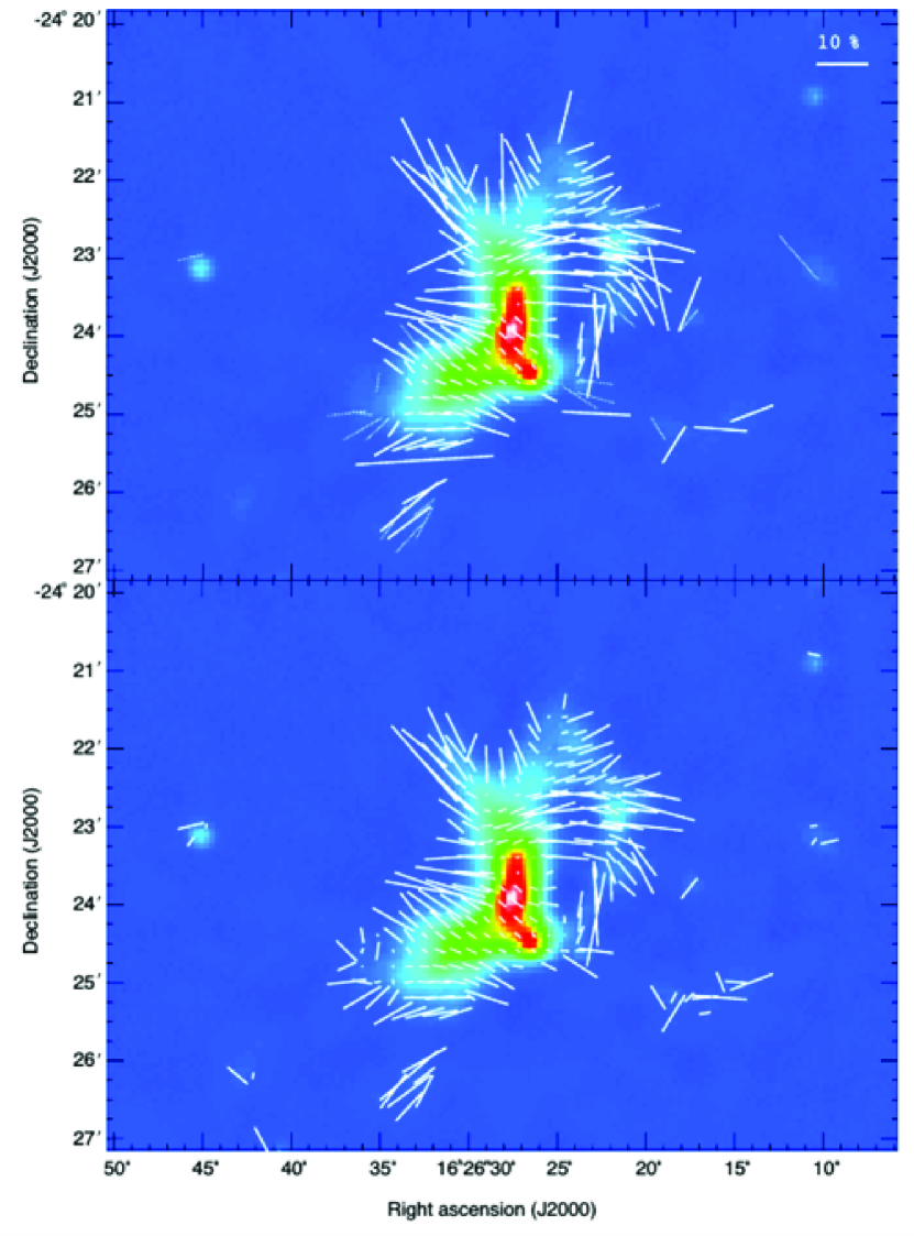
Figure 6: The 850 $\mu$m polarization vector maps, sampled on a 12$\arcsec$ grid and rotated by 90$\arcdeg$ (i.e., as in Figure 3 but rotated by 90$\arcdeg$). The 90$\arcdeg$ rotated vectors, which show the inferred magnetic field orientation projected on the plane of the sky, are plotted where $I>0$, $P/\delta P>2$, and $\delta P<4\%$ (dotted vectors) and $I>0$, $P/\delta P>3$, and $\delta P<4\%$ (solid vectors) in the top panel and where $I>0$ and $I/\delta I>20$ in the bottom panel, respectively. A 10% scale vector is shown in the upper right corner. See text for these two panels with different selections ($P/\delta P$ and $I/\delta I$).

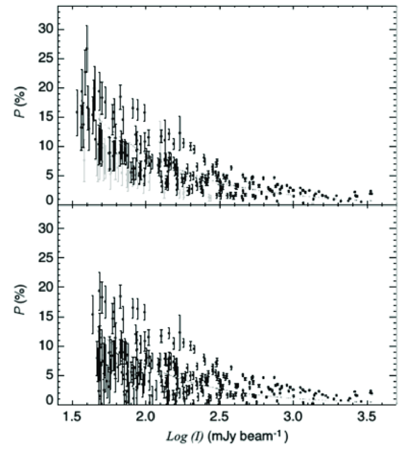
Figure 7: Degree of polarization ($P$) vs. Intensity ($I$). Top panel: Black circles show the sources with $I>0$, $P/\delta P>3$, and $\delta P<4\%$, and grey circles show the sources with $I>0$, $P/\delta P>2$, and $\delta P<4\%$. Bottom panel: Black circles show the sources with $I>0$, $I/\delta I>20$, and $P>0$. Each least-square-fit power-law is shown as dotted curves.

We have found by eye that there are at least 10 distinct magnetic field components in the core region, and we refer to them as “Components a–j” (see Figure 8). Please note that our division of these components does not mean that these field component are always independent but all or some of them could be smoothly connected with eath other. The aim of the region division here is mainly to identify the change of directions and degrees of the polarization vectors and to compare them with the near-infrared polarization data. A summary of these components is as follows:

1. Small $P$ ($<$ 3%) and $\sim$50$\arcdeg$ component at SM 1 and VLA 1623 around the center of the observed field-of-view,

2. Large $P$ and $\sim$40$\arcdeg$ component near A-MM 7 to the east of A-MM 5,

3. Large $P$ and $\sim$20$\arcdeg$ component near A-MM 5,

4. Large $P$ and $\sim$100$\arcdeg$ component at A-MM 4,

5. Small $P$ ($<$ 3%) and $\sim$100$\arcdeg$ component between A-MM 5 and SM 1N,

6. Large $P$ and $\sim$80$\arcdeg$ component to the west of SM 1,

7. Large $P$ and $\sim$70$\arcdeg$ component to the east of SM 1 and SM 1N,

8. Large $P$ and $\sim$80$\arcdeg$ component at A-MM 3,

9. Small $P$ ($<$ 3%) and $\sim$80$\arcdeg$ component between SM 2 and A-MM 8,

10. Large $P$ and $\sim$120$\arcdeg$ component between SM 2 and A-MM 8.

Figure 8 illustrates that these components differ from each other either in polarization position angle or degree of polarization (see also Table 2). Components a, c, and i are already seen in, and are consistent with, SCUPOL data (Tamura, 1999). Components b, d, e, f, g, h, and j are additionally identified in our SCUBA-2/POL-2 data. One can also see the polarization vectors associated with the Components b, d, e, g, and j in Matthews et al. (2009). We also note that our results suggest the magnetic field is mostly well organized (rather than disordered due to turbulence; see Section 5.2).

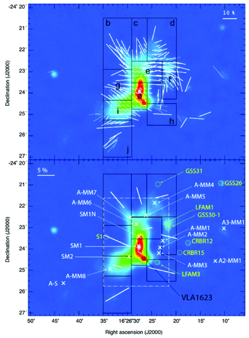
Figure 8: Close up of the $\rho$ Oph-A core region in Figure 1, with regions divided according to the magnetic field direction (top panel), and showing the median of the magnetic field directions of each region shown in Table 2 (bottom panel). Black boxes indicate the Componets a-j (see Section 5.1). 10% and 5% scale vectors are shown in the upper right (top panel) and left (bottom panel) corners, respectively. Note that $P/\delta P>2$ (dotted vectors) and $P/\delta P>3$ (solid vectors) data are shown here, therefore the errors of the polarization vector angle are typically much less than 15$\arcdeg$. The region indicated with the white dash-dotted box in the bottom panel is corresponding to the region shown in Figure 10.

In the central region around SM 1 (Component a), the vectors are well aligned with the 50$\arcdeg$ magnetic field component observed in the surrounding medium on various scales (see Section 5.4). Although the average direction of the main component is approximately 50$\arcdeg$, the magnetic field tends to be locally perpendicular (approximately 100$\arcdeg$–110$\arcdeg$) to the arc-structure (south part of Region f). Between SM 1N and A-MM 6, the magnetic field direction is almost east-west (Component e) while the arc extends to the north-east or north-west, and the magnetic field directions extend toward LFAM1 and GSS 30–1 (Component f). A perpendicular field relative to the core shape (i.e., the elongation of the arc-structure between north-east and north-west filaments) is important for the formation and growth of this core. Such orthogonal fields are often seen in the densest parts of the cloud or cloud cores (Tamura et al., 1987, 1988; Nagai et al., 1998; Palmeirim et al., 2013; Matthews et al., 2014; Fissel et al., 2016; André et al., 2013; Planck Collaboration et al., 2016).

There are other local structures besides the 50$\arcdeg$ component. To the north of A-MM6 (Component c), the magnetic field direction is almost north-south, and to the north of A-MM7, the magnetic field direction is almost north-east (Component b), which is the same as the direction of the north-east filament. Notable are the low degree of polarization near SM 1N and some deviation in magnetic field direction near VLA 1623 and its outflow region.

In this paper, we have assumed that the 850 $\mu$m emission measured by SCUBA-2 is dominated by the thermal dust continuum emission. However, the continuum emission can be contaminated by CO (3–2) line emission (Drabek et al., 2012). Figure 9 shows an overlay of the CO (3–2) line emission from White et al. (2015) on the 850 $\mu$m continuum map. In the dense center of Oph-A, the CO contamination fraction is typically $<1\%$. However, in the brightest regions of CO emission from the outfow from VLA 1623, the contamination fraction can be much higher (Pattle et al., 2015). The regions that have high CO contamination have very low column density values, and are mostly along the jet axis between Oph-B and Oph-C/E/F, outside our field of view. In the dense center of Oph-A, the fractional contribution of CO is $<1\%$ and generally does not exceed 10% anywhere on source. The ring-shaped region seen in our Stokes $I$ image to the west of Oph-A is dominated by the CO emission rather than the thermal dust emission. Since the CO emission is weak toward the bright dust emission ($<5\%$), even if it is polarized by the Goldreich-Kylafis effect, it will contribute minimally to our results.

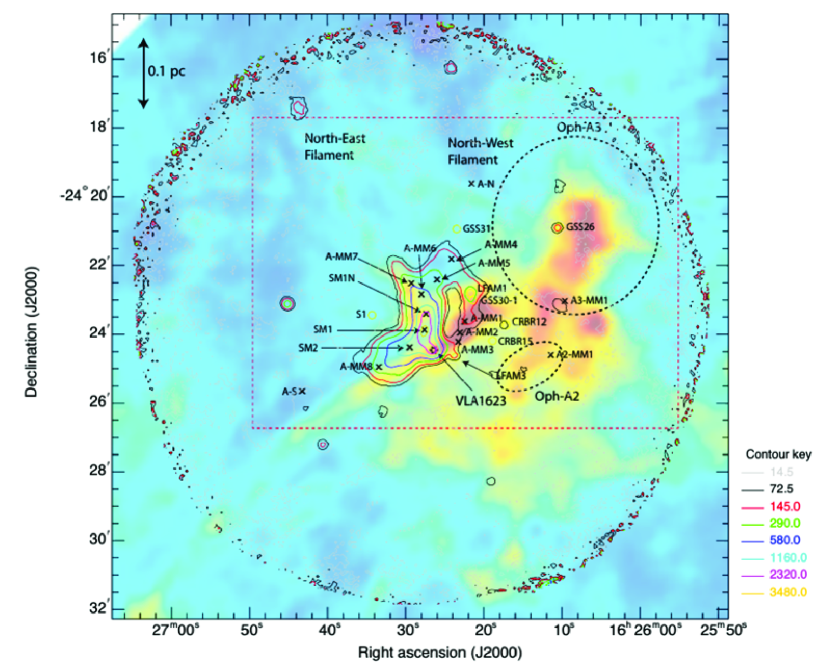
Figure 9: Contours of the 850 $\mu$m total intensity (Stokes $I$) image (cf. Figure 1 of this work) of the $\rho$ Oph-A field superimposed on HARP CO $J=3-2$ observations showing the integrated emission between $-$5 and $+$12 km s^-1 (cf. Figure 1 of White et al. 2015).

5.2 Local Magnetic Field Strength

Polarization arising from dust grains, which are aligned with their major axes perpendicular to the magnetic field (e.g., Hoang & Lazarian 2009), allows us to estimate the magnetic field direction. However, the present uncertainties in theories of dust grain alignment limit the ability with current techniques to trace magnetic fields without ambiguities (see Lazarian, 2007; Lazarian et al., 2015, for a review).

The most common method to infer a magnetic field strength from polarized dust emission is the Davis-Chandrasekhar-Fermi method (more commonly referred as the Chandrasekhar-Fermi (CF) method; Davis 1951; Chandrasekhar & Fermi 1953; see also Houde et al. 2016 and Pattle et al. 2017). The Davis-Chandrasekhar-Fermi method infers a magnetic field strength by statistically comparing the dispersion in the polarization orientation with the dispersion in velocity. Therefore, the magnetic field strength projected on the plane of the sky can be calculated by

$$\begin{split}B_{p}&={\cal Q}\sqrt{4\pi\rho}\ {{\delta v_{\rm los}}\over{\delta\theta}}\\ \end{split}$$ (7)

assuming that velocity perturbations are isotropic (Ostriker et al., 2001). In Equation (7), $\cal Q$ is a factor to account for various averaging effects (see Houde 2004 and Crutcher et al. 2004 for details), $\rho$ is the mean density of the cloud, $\delta v_{\rm los}$ is the rms line-of-sight velocity, and $\delta\theta$ is the dispersion in the polarization angle. To estimate a magnetic field strength in the $\rho$ Oph-A core region, a correction factor of $\cal Q=$0.5 is adopted here because the magnetic field appears to be ordered (Ostriker et al. 2001; Houde 2004, also see Falceta-Gonçalves et al. 2008; Novak et al. 2009; Pattle et al. 2017). Since we apply this formula only to the sub-regions where the angle dispersion is relatively small ($\leq 25\arcdeg$) and the velocity dispersion of the molecular lines tracing high density regions is available in the next paragraph, $\cal Q$ = 0.5 is appropriate, as simulated by Ostriker et al. (2001). Note that if the turbulence correlation length is not resolved and therefore their simulation assumption is not valid, the case the $\cal Q$ factor can be much lower (Heitsch et al. 2001, see also Houde et al. 2009). Then Equation (7) can be expressed as follows (Lai et al., 2002):

$$\begin{split}B_{p}&=8.5{\sqrt{n_{\rm H2}/(10^{6}\,\rm cm^{-3})}\,\Delta v/(\rm km\,s^{-1})\over{\delta\theta(\arcdeg)}}\rm\,mG\end{split}$$ (8)

Here, $n_{\rm H_{2}}$ is the number density of hydrogen molecules and $\Delta v$ is the line width.

As mentioned in previous section, there are several magnetic field components in the $\rho$ Oph-A core region. Since they are different from each other either in direction or degree of polarization, we estimate the magnetic field strength of each component separately. To investigate their magnetic field strengths individually, we estimated median polarization position angles, which indicate the local average magnetic field directions of each component. Table 2 shows the median degrees of polarizations and position angles calculated using Stokes $Q$ and $U$ in each region. Figure 8 shows the vectors in each region averaged over in each region.

The local average density in each of the Components a–j is calculated from our Stokes $I$ data, assuming that the core-depth is equal to the geometric mean size of each sub-core where the polarization data exist, and ranges from $2\times 10^{6}$ cm^-3 to $7\times 10^{4}$ cm^-3. Since the $\rho$ Oph-A core has a complex magnetic field structure showing various directions in each sub-core, we do not attempt to apply to the Davis-Chandrasekhar-Fermi method to the entire core but only to the sub-cores showing a relatively well-defined magnetic field direction. In Components a, d and e, André et al. (2007) estimated a velocity dispersion of 0.26 km s^-1, 0.15 km s^-1, and 0.17 km s^-1, respectively. These are non-thermal line dispersions from N₂H⁺ (1–0) observations. Using these values with the standard deviation in field direction of 1.5$\arcdeg$, 5.8$\arcdeg$, and 2.7$\arcdeg$ found in each region, the magnetic field strength projected on the plane of the sky is calculated as $Bp\sim$ 5, 0.2, and 0.8 mG (cf. Table 2). The estimated magnetic field strength in the $\rho$ Oph-A core region is larger than that in other molecular clouds derived using the Davis-Chandrasekhar-Fermi method (namely 20–200 $\mu$G; Andersson & Potter 2005; Poidevin & Bastien 2006; Alves et al. 2008; Kwon et al. 2010, 2011; Sugitani et al. 2011; Kusune et al. 2015) but comparable to those in the Orion A region (see e.g., Pattle et al. 2017). Our high magnetic field strengths may be attributed to using the higher H₂ densities associated with the sub-cores rather than the lower H₂ densities associated with the larger $\rho$ Oph-A core. Thus, we conservatively take these field strengths as an order-of-magnitude estimate. These values are still representative of the field strength toward the sub-cores in $\rho$ Oph-A and can be taken as an upper limit for the surrounding gas.

Finally, it should be noted that there are certain limitations in the Davis-Chandrasekhar-Fermi technique such as the effect of the limited telescope resolution (Heitsch et al., 2001). Also note that our estimates are only for some sub-regions where the field dispersions are relatively small. Therefore, both of these effects tend to bias towards a high magnetic field strength. In addition, more sophisticated applications of the Davis-Chandrasekhar-Fermi technique such as described in Pattle et al. (2017) or Hildebrand et al. (2009) would be desirable in future works.

5.3 Magnetic Fields and Centroid Velocity

Our polarimetric data will be useful to discuss the correlation between the magnetic field and the velocity field in each core. However, this will be beyond the scope of this first-look paper. Therefore, in this section, we show an example of a possible correlation between magnetic field and velocity gradient.

Strong Alfvénic turbulence develops eddy-like motions perpendicular to the local magnetic field direction (Goldreich & Sridhar, 1995). Very recently, González-Casanova & Lazarian (2017) have proposed that this fact can be used to study the direction of magnetic fields by using the velocity gradient calculated from the centroid velocity. The centroid velocity is an intensity-weighted average velocity along the line of sight (e.g., Miesch et al. 1999). Here, we try to compare the magnetic field direction in the $\rho$ Oph-A core region with centroid velocity components.

André et al. (2007) measured subsonic or transonic levels of internal turbulence within the condensations, and their result supports the view that most of the L1688 starless condensations are gravitationally bound and prestellar in nature. Figure 10 shows a comparison between magnetic field direction (this work) and centroid velocity components of N₂H⁺(1–0) spectra (André et al., 2007). The apparent main velocity core gradient (indicated by arrows in Figure 10) appears to be roughly perpendicular to the magnetic field orientation traced by POL-2. Certainly these observations should be compared with theoretical modeling using the physical parameters of the $\rho$ Oph-A core in future.

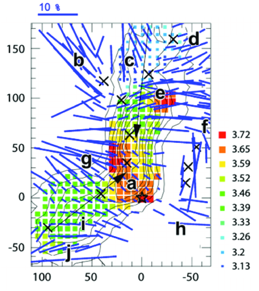
Figure 10: Comparison between magnetic field directions from this work and the centroid velocity components of N₂H⁺(1–0) spectra (filled squares of varying sizes and colors, Figure 6(c) of André et al. 2007). The (0, 0) offset corresponds to the position $\alpha$ = 16^h 26^m 26$\fs$45, $\delta$ = -24$\arcdeg$ 24$\arcmin$ 30.8$\arcsec$ [J2000]. The contours, which were drawn by André et al. (2007), go from 2 to 16 K km s^-1. The color code shows the velocity centroid. The underlying contours represent the same N₂H⁺(1–0) integrated intensity maps. Our suggested centroid velocity gradient is shown by black arrows, which are not in the original figure (André et al., 2007). Shown in the upper left is the 10% scale vector for the 90$\arcdeg$-rotated submillimeter polarization vectors. The letters a–j are the magnetic field components defined from our submillimeter polarimetry (see text). Crosses mark the 1.2 mm continuum positions of starless condensations, while stars mark the positions of VLA 1623 (see André et al. 2007). The labels a–j indicate the distinct magnetic field components in each sub-region a–j.

5.4 Tracing magnetic fields across different wavelengths

Polarimetry in the $\rho$ Oph-A core region was reported previously by several authors at other wavelengths. Sato et al. (1988) carried out near-infrared polarimetry (in the $K$ band only) of 20 sources which are embedded within the densest region of the $\rho$ Oph dark cloud with a single channel detector, and they suggested that there are three dominant components of the polarization position angles 0°, 50°, and 150°. Recently, Kwon et al. (2015) presented wide and deep near-infrared polarimetry (in the $JHK_{s}$ bands) of the $\rho$ Oph regions, which corresponds to the densest part of L1688. Since they cover a wider region than our observations (but much more sparsely due to the limited number of stars available for the aperture polarimetry), we compare their polarimetry data covering a 40′$\times$ 40′region with our submillimeter data. In this active cluster-forming region, they found that the magnetic fields appear to be connected from core to core, rather than as a simple overlap of the different cloud core components. Putting it differently, the magnetic field morphology seems to be connected between different cores in the $\rho$ Oph molecular cloud complex. In addition, comparing their near-infrared polarimetric results with the large-scale magnetic field structures obtained from previous optical polarimetric study (Vrba et al., 1976), they suggested that the magnetic field structures in the $\rho$ Oph core were distorted by the cluster formation in this region, which may have been induced by shock compression due to wind/radiation from the Scorpius–Centaurus association. Also note that there is 350 $\mu$m submillimeter polarization from the CSO in Dotson et al. (2010) for $\rho$ Oph-A. Their data are broadly consistent with our 850 $\mu$m map.

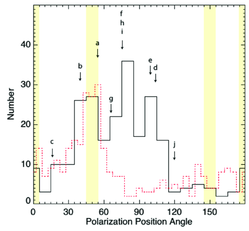
Figure 11: Histogram of polarization position angles for the 90$\arcdeg$-rotated submillimeter vectors with $I>0$, $P/\delta P>2$, and $\delta P<4\%$ (black). Black line: 90$\arcdeg$ rotated submillimeter polarization vectors (this work). Note that a 10$\arcdeg$ bin is used. Red dotted line: $H$-band polarization position angles (Kwon et al., 2015). Black arrows indicate the magnetic field components from the submillimeter data. The labels a–j indicate the average magnetic field direction of the distinct magnetic field components a–j projected on the plane of the sky. Yellow colored regions indicate the major magnetic field directions suggested from the previous near-infrared data.

Our new submillimeter polarimetry demonstrates that one of the main polarization position angles in Oph-A are approximately 50$\arcdeg$ (see Figures 3–10), and so are well aligned with the 50$\arcdeg$ magnetic field found in the near-infrared (Kwon et al. 2015; see also Figure 5 for their comparison within the same field-of-view). Kwon et al. (2015) found that the “50$\arcdeg$ component” is the dominant magnetic field component in the observed region; it can be seen as a distinct clump in the diagram plotting degree of polarization versus polarization angle (Figure 9 of Kwon et al. 2015) and in the histogram of polarization position angles (Figure 10 of Kwon et al. 2015). This component is seen in the northeast regions of $\rho$ Oph-A (and in $\rho$ Oph-B and $\rho$ Oph-E in a large scale, regions not covered in this work). The “0$\arcdeg$ component” can be seen from $\rho$ Oph-A toward $\rho$ Oph-AC (located at the southeastern region of $\rho$ Oph-A, which is not shown in our submillimeter map; cf. Kwon et al. 2015). In contrast, in Oph-A, both the 0$\arcdeg$ and the 50$\arcdeg$ components exist.

Figure 11 shows the histogram of polarization position angles for the 90$\arcdeg$ rotated submillimeter polarization vectors as well as for the $H$-band polarization position angles from Kwon et al. (2015). The distribution is relatively widespread, but if we refer to both the $H$-band polarization vector map (Figure 8 of Kwon et al. 2015) and this histogram, we see several components, of which the components at 0°and 50$\arcdeg$ are most clearly seen. As shown in Figure 11, the distribution of the polarization position angles obtained from submillimeter polarimetry is in relatively good agreement with those obtained from near-infrared polarimetry for the 0$\arcdeg$ and 50$\arcdeg$ components but not for the 150$\arcdeg$ component. Note that since our submillimeter map covers a small part of the area covered by the near-infrared polarimetry survey and we see much higher-column-density regions of $\rho$ Oph-A, there is also some inconsistency between the distributions of submillimeter and near-infrared polarization angles. Therefore, our results indicate that both submillimeter emission polarization and near-infrared dichroic polarization may trace the magnetic field structures associated with the $\rho$ Oph-A core region at different spatial scales and at different region along the line-of-sight.

Previous observations have shown agreement between the magnetic field structures seen at various wavelengths such as near- and far-infrared, or submillimeter wavelengths (e.g., Tamura et al., 1996, 2007; Kandori et al., 2007; Kwon et al., 2011). Our new results are consistent with this behavior, although the greatest density regions can be traced only by submillimeter polarimetry. The 50$\arcdeg$ component seen in the lower-density regions of the submillimeter map around the edge of the core (the north-east filament, cf. Figure 1) is consistent with the 50$\arcdeg$ component seen in the lower-density tracer of near-infrared polarization (Kwon et al., 2015), giving us still further confidence in our observations. Our data are also consistent with the recently released HAWC+ data taken by SOFIA (Santos et al., 2018). A combination of polarimetric observations over wavelengths and scales observed by instruments such as ALMA and by 8-m class optical/infrared telescopes will become more important in the future, to test the range of scales over which this behavior holds.

6 SUMMARY

In this paper, we present the first-look analysis for the $\rho$ Oph-A SCUBA-2/POL-2 continuum map observed by the JCMT Gould Belt polarization survey at 850 $\mu$m. The $\rho$ Oph molecular cloud complex is one of the nearest laboratories for examining active star-formation sites, offering a wealth of objects to aid in a better understanding of the dominant physical processes present in the region. The SCUBA-2/POL-2 polarimeter is a very powerful instrument to trace the magnetic eld structure in star forming regions such as the Oph molecular cloud complex. The main results are as follows.

1. We have identified at least 10 magnetic field components in the $\rho$ Oph-A core region, whose position angles and degrees of polarization are distinct from each other. However, some of them can be part of a coherent structure. Our polarimetric results are not only consistent with previous results in the bright core regions, but also reveal the fields in the outer regions for the first time. These components represent the magnetic fields of the sub-cores identified as local continuum intensity peaks or distinct velocity structures within the Oph-A core; they show a large variation even within the small (approximately 0.2 pc) region observed.

2. The dominant component of the magnetic field over $\rho$ Oph-A is the 50$\arcdeg$ component. This direction is consistent with that inferred from the near-infrared polarimetry of the $\rho$ Oph cloud core.

3. Although the average direction of the main component is approximately 50$\arcdeg$, the magnetic field tends to be locally perpendicular (approximately 100$\arcdeg$–110$\arcdeg$) to the arc-structure. Between SM 1N and A-MM 6, the field direction is almost east-west, while the arc extends to the north-east or north-west, and the field direction extends toward LFAM 1 and GSS 30–1. The perpendicularity between the core shape and the magnetic field direction may be important in understanding the origin and formation of this core. Such perpendicularity is often seen in the densest parts of clouds and cloud cores.

4. There are local structures besides the 50$\arcdeg$ component. To the north of A-MM 6, the field direction is almost north-south, and to the north of A-MM 7, the field direction is almost north-east, which is the same of the direction of the north-east filament. Notable are the low degree of polarization near SM 1N and some deviation in field direction near VLA 1623 and its outflow region.

5. Using the Davis-Chandrasekhar-Fermi method, we roughly estimate the strengths of the magnetic field projected on the plane of the sky in several sub-core regions to be up to a few mG.

6. We have found that the main large-scale core velocity gradient is approximately perpendicular to the inferred cloud magnetic field orientation.

Table 1: Submillimeter Polarimetry in the $\rho$ Ophiuchi Cloud Core

ID	Position		$I\pm\delta I$	$Q\pm\delta Q$	$U\pm\delta U$	$P\pm\delta P$	$\theta\pm\delta\theta$	Component
	$\alpha_{\rm J2000}$	$\delta_{\rm J2000}$	(mJy/beam)	(mJy/beam)	(mJy/beam)	(%)	(°)
1	16:26:33.4	-24:26:35.10	51.430 $\pm$ 2.098	-0.342 $\pm$ 1.619	4.101 $\pm$ 1.608	7.37 $\pm$ 3.14	47.4 $\pm$ 11.3	j
2	16:26:34.3	-24:26:23.10	58.272 $\pm$ 2.122	-1.394 $\pm$ 1.615	4.885 $\pm$ 1.616	8.26 $\pm$ 2.79	53.0 $\pm$ 9.1	j
3	16:26:32.5	-24:26:23.10	62.223 $\pm$ 2.095	-2.642 $\pm$ 1.595	3.811 $\pm$ 1.592	7.00 $\pm$ 2.57	62.4 $\pm$ 9.8	j
4	16:26:33.4	-24:26:23.10	67.742 $\pm$ 2.103	2.010 $\pm$ 1.603	6.867 $\pm$ 1.597	10.30 $\pm$ 2.38	36.8 $\pm$ 6.4	j
5	16:26:33.4	-24:26:11.10	69.851 $\pm$ 2.038	1.644 $\pm$ 1.576	10.126 $\pm$ 1.563	14.51 $\pm$ 2.28	40.4 $\pm$ 4.4	j
6	16:26:32.5	-24:26:11.10	74.294 $\pm$ 2.043	1.045 $\pm$ 1.552	4.014 $\pm$ 1.556	5.18 $\pm$ 2.10	37.7 $\pm$ 10.7	j
7	16:26:32.5	-24:25:59.10	50.015 $\pm$ 2.039	2.705 $\pm$ 1.519	4.317 $\pm$ 1.510	9.73 $\pm$ 3.05	29.0 $\pm$ 8.5	j
8	16:26:32.5	-24:25:35.10	39.887 $\pm$ 2.062	10.629 $\pm$ 1.467	1.343 $\pm$ 1.482	26.61 $\pm$ 3.93	3.6 $\pm$ 4.0	j
9	16:26:34.3	-24:25:23.10	61.159 $\pm$ 2.082	2.735 $\pm$ 1.496	4.664 $\pm$ 1.506	8.49 $\pm$ 2.48	29.8 $\pm$ 7.9	j
10	16:26:33.4	-24:25:23.10	106.577 $\pm$ 2.065	5.813 $\pm$ 1.473	4.804 $\pm$ 1.484	6.94 $\pm$ 1.39	19.8 $\pm$ 5.6	j
11	16:26:32.5	-24:25:23.10	136.809 $\pm$ 2.039	9.366 $\pm$ 1.450	5.233 $\pm$ 1.458	7.77 $\pm$ 1.07	14.6 $\pm$ 3.9	j
12	16:26:30.8	-24:25:23.10	140.545 $\pm$ 2.035	7.720 $\pm$ 1.442	5.518 $\pm$ 1.452	6.67 $\pm$ 1.03	17.8 $\pm$ 4.4	j
13	16:26:31.6	-24:25:23.10	158.406 $\pm$ 2.045	10.415 $\pm$ 1.443	3.233 $\pm$ 1.449	6.82 $\pm$ 0.92	8.6 $\pm$ 3.8	j
14	16:26:18.5	-24:25:23.08	60.328 $\pm$ 2.255	-2.298 $\pm$ 1.482	4.702 $\pm$ 1.505	8.31 $\pm$ 2.51	58.0 $\pm$ 8.1	$\cdots$
15	16:26:29.0	-24:25:11.10	72.854 $\pm$ 2.037	5.357 $\pm$ 1.399	-3.862 $\pm$ 1.396	8.86 $\pm$ 1.94	-17.9 $\pm$ 6.1	$\cdots$
16	16:26:34.3	-24:25:11.10	163.985 $\pm$ 2.057	-2.271 $\pm$ 1.473	5.622 $\pm$ 1.495	3.58 $\pm$ 0.91	56.0 $\pm$ 7.0	i
17	16:26:29.9	-24:25:11.10	179.956 $\pm$ 2.042	1.486 $\pm$ 1.404	-3.252 $\pm$ 1.405	1.83 $\pm$ 0.78	-32.7 $\pm$ 11.3	i
18	16:26:33.4	-24:25:11.10	243.825 $\pm$ 2.065	5.194 $\pm$ 1.455	0.295 $\pm$ 1.469	2.05 $\pm$ 0.60	1.6 $\pm$ 8.1	i
19	16:26:32.5	-24:25:11.10	263.398 $\pm$ 2.060	11.865 $\pm$ 1.441	0.168 $\pm$ 1.450	4.47 $\pm$ 0.55	0.4 $\pm$ 3.5	i
20	16:26:31.6	-24:25:11.10	285.549 $\pm$ 2.022	15.906 $\pm$ 1.409	2.776 $\pm$ 1.435	5.63 $\pm$ 0.50	5.0 $\pm$ 2.5	i
21	16:26:30.8	-24:25:11.10	296.876 $\pm$ 2.016	16.204 $\pm$ 1.409	1.031 $\pm$ 1.408	5.45 $\pm$ 0.48	1.8 $\pm$ 2.5	i
22	16:26:36.0	-24:25:11.09	52.454 $\pm$ 2.123	2.267 $\pm$ 1.542	4.078 $\pm$ 1.549	8.39 $\pm$ 2.97	30.5 $\pm$ 9.5	$\cdots$
23	16:26:35.2	-24:25:11.09	64.541 $\pm$ 2.038	0.240 $\pm$ 1.505	4.359 $\pm$ 1.504	6.35 $\pm$ 2.34	43.4 $\pm$ 9.9	$\cdots$
24	16:26:19.3	-24:25:11.08	57.627 $\pm$ 2.173	-1.546 $\pm$ 1.457	-2.992 $\pm$ 1.477	5.26 $\pm$ 2.57	-58.7 $\pm$ 12.4	$\cdots$
25	16:26:15.8	-24:25:11.06	48.901 $\pm$ 2.371	5.178 $\pm$ 1.543	-0.781 $\pm$ 1.566	10.23 $\pm$ 3.20	-4.3 $\pm$ 8.6	$\cdots$
26	16:26:28.1	-24:24:59.10	79.582 $\pm$ 2.088	2.094 $\pm$ 1.378	-4.110 $\pm$ 1.383	5.53 $\pm$ 1.74	-31.5 $\pm$ 8.6	$\cdots$
27	16:26:29.0	-24:24:59.10	209.209 $\pm$ 2.086	7.624 $\pm$ 1.374	-7.347 $\pm$ 1.388	5.02 $\pm$ 0.66	-22.0 $\pm$ 3.7	$\cdots$
28	16:26:34.3	-24:24:59.10	275.086 $\pm$ 2.023	-3.445 $\pm$ 1.464	-0.868 $\pm$ 1.472	1.18 $\pm$ 0.53	-82.9 $\pm$ 11.9	i
29	16:26:33.4	-24:24:59.10	407.349 $\pm$ 2.051	7.166 $\pm$ 1.441	2.139 $\pm$ 1.454	1.80 $\pm$ 0.35	8.3 $\pm$ 5.6	i
30	16:26:29.9	-24:24:59.10	421.360 $\pm$ 2.050	9.406 $\pm$ 1.387	-10.463 $\pm$ 1.378	3.32 $\pm$ 0.33	-24.0 $\pm$ 2.8	i
31	16:26:30.8	-24:24:59.10	472.817 $\pm$ 2.054	19.633 $\pm$ 1.387	-6.862 $\pm$ 1.412	4.39 $\pm$ 0.29	-9.6 $\pm$ 1.9	i
32	16:26:32.5	-24:24:59.10	506.147 $\pm$ 2.067	14.517 $\pm$ 1.422	-3.031 $\pm$ 1.424	2.92 $\pm$ 0.28	-5.9 $\pm$ 2.8	i
33	16:26:31.6	-24:24:59.10	535.088 $\pm$ 2.043	20.017 $\pm$ 1.408	-4.015 $\pm$ 1.409	3.81 $\pm$ 0.26	-5.7 $\pm$ 2.0	i
34	16:26:22.9	-24:24:59.09	36.637 $\pm$ 2.072	4.997 $\pm$ 1.386	-0.534 $\pm$ 1.386	13.19 $\pm$ 3.86	-3.1 $\pm$ 7.9	h
35	16:26:36.9	-24:24:59.09	48.555 $\pm$ 2.180	3.892 $\pm$ 1.580	0.981 $\pm$ 1.573	7.60 $\pm$ 3.27	7.1 $\pm$ 11.2	$\cdots$
36	16:26:36.0	-24:24:59.09	105.173 $\pm$ 2.056	4.079 $\pm$ 1.527	-1.656 $\pm$ 1.529	3.93 $\pm$ 1.45	-11.0 $\pm$ 9.9	$\cdots$
37	16:26:14.1	-24:24:59.05	56.258 $\pm$ 2.532	3.874 $\pm$ 1.604	3.473 $\pm$ 1.615	8.80 $\pm$ 2.89	20.9 $\pm$ 8.9	$\cdots$
38	16:26:25.5	-24:24:47.10	128.626 $\pm$ 2.111	2.576 $\pm$ 1.331	-3.453 $\pm$ 1.347	3.18 $\pm$ 1.04	-26.6 $\pm$ 8.9	h
39	16:26:27.3	-24:24:47.10	315.284 $\pm$ 2.174	6.195 $\pm$ 1.357	-1.949 $\pm$ 1.352	2.01 $\pm$ 0.43	-8.7 $\pm$ 6.0	$\cdots$
40	16:26:28.1	-24:24:47.10	322.238 $\pm$ 2.094	3.581 $\pm$ 1.354	-9.384 $\pm$ 1.351	3.09 $\pm$ 0.42	-34.6 $\pm$ 3.9	$\cdots$
41	16:26:33.4	-24:24:47.10	448.077 $\pm$ 2.046	6.608 $\pm$ 1.425	-0.974 $\pm$ 1.431	1.46 $\pm$ 0.32	-4.2 $\pm$ 6.1	i
42	16:26:29.0	-24:24:47.10	505.237 $\pm$ 2.110	9.237 $\pm$ 1.360	-16.107 $\pm$ 1.369	3.67 $\pm$ 0.27	-30.1 $\pm$ 2.1	$\cdots$
43	16:26:32.5	-24:24:47.10	608.888 $\pm$ 2.048	12.679 $\pm$ 1.403	-2.942 $\pm$ 1.413	2.13 $\pm$ 0.23	-6.5 $\pm$ 3.1	i
44	16:26:29.9	-24:24:47.10	781.876 $\pm$ 2.061	20.867 $\pm$ 1.368	-17.607 $\pm$ 1.377	3.49 $\pm$ 0.18	-20.1 $\pm$ 1.4	i
45	16:26:31.6	-24:24:47.10	834.935 $\pm$ 2.056	24.301 $\pm$ 1.389	-9.222 $\pm$ 1.397	3.11 $\pm$ 0.17	-10.4 $\pm$ 1.5	i
46	16:26:30.8	-24:24:47.10	834.771 $\pm$ 2.034	21.231 $\pm$ 1.376	-13.423 $\pm$ 1.377	3.00 $\pm$ 0.17	-16.2 $\pm$ 1.6	i
47	16:26:22.9	-24:24:47.09	38.256 $\pm$ 2.075	2.747 $\pm$ 1.353	-1.657 $\pm$ 1.371	7.60 $\pm$ 3.58	-15.6 $\pm$ 12.2	h
48	16:26:23.7	-24:24:47.09	46.716 $\pm$ 2.083	1.630 $\pm$ 1.347	-3.585 $\pm$ 1.355	7.92 $\pm$ 2.92	-32.8 $\pm$ 9.8	h
49	16:26:33.4	-24:24:35.10	375.056 $\pm$ 2.013	-1.943 $\pm$ 1.399	-5.926 $\pm$ 1.412	1.62 $\pm$ 0.38	-54.1 $\pm$ 6.4	i
50	16:26:32.5	-24:24:35.10	550.300 $\pm$ 2.058	3.323 $\pm$ 1.387	-6.657 $\pm$ 1.393	1.33 $\pm$ 0.25	-31.7 $\pm$ 5.3	i
51	16:26:25.5	-24:24:35.10	553.396 $\pm$ 2.136	5.956 $\pm$ 1.308	-5.067 $\pm$ 1.317	1.39 $\pm$ 0.24	-20.2 $\pm$ 4.8	h
52	16:26:31.6	-24:24:35.10	930.155 $\pm$ 2.048	16.612 $\pm$ 1.368	-14.349 $\pm$ 1.370	2.36 $\pm$ 0.15	-20.4 $\pm$ 1.8	i
53	16:26:28.1	-24:24:35.10	1003.480 $\pm$ 2.149	9.105 $\pm$ 1.330	-12.010 $\pm$ 1.332	1.50 $\pm$ 0.13	-26.4 $\pm$ 2.5	a
54	16:26:29.0	-24:24:35.10	1119.110 $\pm$ 2.061	17.792 $\pm$ 1.332	-14.137 $\pm$ 1.336	2.03 $\pm$ 0.12	-19.2 $\pm$ 1.7	a
55	16:26:30.8	-24:24:35.10	1174.260 $\pm$ 2.021	20.439 $\pm$ 1.352	-20.801 $\pm$ 1.362	2.48 $\pm$ 0.12	-22.8 $\pm$ 1.3	i
56	16:26:29.9	-24:24:35.10	1282.560 $\pm$ 2.076	19.135 $\pm$ 1.338	-24.433 $\pm$ 1.349	2.42 $\pm$ 0.10	-26.0 $\pm$ 1.2	i
57	16:26:27.3	-24:24:35.10	1371.780 $\pm$ 2.362	7.661 $\pm$ 1.329	-11.563 $\pm$ 1.319	1.01 $\pm$ 0.10	-28.2 $\pm$ 2.7	a
58	16:26:26.4	-24:24:35.10	1887.860 $\pm$ 2.594	3.423 $\pm$ 1.319	-17.786 $\pm$ 1.322	0.96 $\pm$ 0.07	-39.6 $\pm$ 2.1	a
59	16:26:22.9	-24:24:35.09	47.454 $\pm$ 2.053	3.372 $\pm$ 1.335	-0.894 $\pm$ 1.355	6.79 $\pm$ 2.83	-7.4 $\pm$ 11.1	h
60	16:26:35.2	-24:24:35.09	96.748 $\pm$ 2.068	-3.614 $\pm$ 1.467	1.021 $\pm$ 1.481	3.57 $\pm$ 1.52	82.1 $\pm$ 11.3	$\cdots$
61	16:26:23.7	-24:24:35.09	168.924 $\pm$ 2.043	3.591 $\pm$ 1.313	0.056 $\pm$ 1.332	1.98 $\pm$ 0.78	0.4 $\pm$ 10.6	h
62	16:26:34.3	-24:24:23.10	162.147 $\pm$ 2.032	1.783 $\pm$ 1.437	-7.161 $\pm$ 1.433	4.46 $\pm$ 0.89	-38.0 $\pm$ 5.6	i
63	16:26:33.4	-24:24:23.10	333.190 $\pm$ 2.020	-2.890 $\pm$ 1.380	-10.016 $\pm$ 1.409	3.10 $\pm$ 0.42	-53.0 $\pm$ 3.8	i
64	16:26:32.5	-24:24:23.10	534.381 $\pm$ 1.993	1.523 $\pm$ 1.365	-8.430 $\pm$ 1.379	1.58 $\pm$ 0.26	-39.9 $\pm$ 4.6	i
65	16:26:25.5	-24:24:23.10	778.337 $\pm$ 2.115	-0.120 $\pm$ 1.295	-5.106 $\pm$ 1.291	0.63 $\pm$ 0.17	-45.7 $\pm$ 7.3	$\cdots$
66	16:26:31.6	-24:24:23.10	816.746 $\pm$ 2.022	4.701 $\pm$ 1.351	-20.827 $\pm$ 1.353	2.61 $\pm$ 0.17	-38.6 $\pm$ 1.8	i
67	16:26:30.8	-24:24:23.10	1158.130 $\pm$ 1.998	11.575 $\pm$ 1.341	-27.026 $\pm$ 1.337	2.54 $\pm$ 0.12	-33.4 $\pm$ 1.3	i
68	16:26:29.9	-24:24:23.10	1493.050 $\pm$ 2.017	12.956 $\pm$ 1.320	-31.557 $\pm$ 1.326	2.28 $\pm$ 0.09	-33.8 $\pm$ 1.1	i
69	16:26:29.0	-24:24:23.10	1660.180 $\pm$ 2.071	8.695 $\pm$ 1.314	-23.456 $\pm$ 1.304	1.50 $\pm$ 0.08	-34.8 $\pm$ 1.5	a
70	16:26:28.1	-24:24:23.10	1964.770 $\pm$ 2.153	3.659 $\pm$ 1.314	-30.492 $\pm$ 1.312	1.56 $\pm$ 0.07	-41.6 $\pm$ 1.2	a
71	16:26:26.4	-24:24:23.10	2416.880 $\pm$ 2.535	-4.410 $\pm$ 1.289	-25.770 $\pm$ 1.303	1.08 $\pm$ 0.05	-49.9 $\pm$ 1.4	a
72	16:26:27.3	-24:24:23.10	2643.620 $\pm$ 2.315	4.500 $\pm$ 1.290	-42.859 $\pm$ 1.297	1.63 $\pm$ 0.05	-42.0 $\pm$ 0.9	a
73	16:26:23.7	-24:24:23.09	136.669 $\pm$ 2.065	-3.840 $\pm$ 1.302	3.425 $\pm$ 1.307	3.64 $\pm$ 0.96	69.1 $\pm$ 7.3	$\cdots$
74	16:26:34.3	-24:24:11.10	86.585 $\pm$ 2.059	4.128 $\pm$ 1.419	-6.984 $\pm$ 1.433	9.22 $\pm$ 1.67	-29.7 $\pm$ 5.0	g
75	16:26:33.4	-24:24:11.10	200.755 $\pm$ 2.019	1.662 $\pm$ 1.381	-9.789 $\pm$ 1.392	4.90 $\pm$ 0.70	-40.2 $\pm$ 4.0	g
76	16:26:32.5	-24:24:11.10	354.117 $\pm$ 1.999	-0.931 $\pm$ 1.355	-17.182 $\pm$ 1.359	4.84 $\pm$ 0.38	-46.6 $\pm$ 2.3	g
77	16:26:31.6	-24:24:11.10	454.205 $\pm$ 1.989	3.053 $\pm$ 1.323	-22.731 $\pm$ 1.347	5.04 $\pm$ 0.30	-41.2 $\pm$ 1.7	g
78	16:26:25.5	-24:24:11.10	473.293 $\pm$ 2.094	1.082 $\pm$ 1.276	-8.387 $\pm$ 1.288	1.77 $\pm$ 0.27	-41.3 $\pm$ 4.3	f
79	16:26:30.8	-24:24:11.10	627.260 $\pm$ 2.010	3.335 $\pm$ 1.322	-28.680 $\pm$ 1.329	4.60 $\pm$ 0.21	-41.7 $\pm$ 1.3	g
80	16:26:29.9	-24:24:11.10	953.887 $\pm$ 2.014	9.991 $\pm$ 1.303	-26.395 $\pm$ 1.314	2.96 $\pm$ 0.14	-34.6 $\pm$ 1.3	g
81	16:26:26.4	-24:24:11.10	1417.450 $\pm$ 2.182	11.137 $\pm$ 1.272	-24.760 $\pm$ 1.281	1.91 $\pm$ 0.09	-32.9 $\pm$ 1.3	a
82	16:26:29.0	-24:24:11.10	1576.900 $\pm$ 2.115	1.175 $\pm$ 1.300	-26.510 $\pm$ 1.300	1.68 $\pm$ 0.08	-43.7 $\pm$ 1.4	a
83	16:26:27.3	-24:24:11.10	2618.600 $\pm$ 2.216	6.129 $\pm$ 1.275	-57.370 $\pm$ 1.284	2.20 $\pm$ 0.05	-42.0 $\pm$ 0.6	a
84	16:26:28.1	-24:24:11.10	2697.520 $\pm$ 2.215	-6.913 $\pm$ 1.285	-40.965 $\pm$ 1.300	1.54 $\pm$ 0.05	-49.8 $\pm$ 0.9	a
85	16:26:22.9	-24:24:11.09	50.474 $\pm$ 2.353	-8.634 $\pm$ 1.307	3.476 $\pm$ 1.310	18.26 $\pm$ 2.73	79.0 $\pm$ 4.0	f
86	16:26:23.7	-24:24:11.09	127.343 $\pm$ 2.063	-6.138 $\pm$ 1.283	1.183 $\pm$ 1.297	4.80 $\pm$ 1.01	84.5 $\pm$ 5.9	f
87	16:26:33.4	-24:23:59.10	68.829 $\pm$ 2.028	-1.088 $\pm$ 1.388	-3.856 $\pm$ 1.393	5.46 $\pm$ 2.03	-52.9 $\pm$ 9.9	g
88	16:26:32.5	-24:23:59.10	144.438 $\pm$ 1.971	3.840 $\pm$ 1.353	-11.073 $\pm$ 1.367	8.06 $\pm$ 0.95	-35.4 $\pm$ 3.3	g
89	16:26:31.6	-24:23:59.10	201.312 $\pm$ 1.996	7.689 $\pm$ 1.324	-18.711 $\pm$ 1.332	10.03 $\pm$ 0.67	-33.8 $\pm$ 1.9	g
90	16:26:25.5	-24:23:59.10	254.610 $\pm$ 2.083	9.190 $\pm$ 1.261	-3.073 $\pm$ 1.279	3.77 $\pm$ 0.50	-9.2 $\pm$ 3.8	f
91	16:26:30.8	-24:23:59.10	300.531 $\pm$ 2.007	8.665 $\pm$ 1.317	-18.943 $\pm$ 1.315	6.92 $\pm$ 0.44	-32.7 $\pm$ 1.8	g
92	16:26:29.9	-24:23:59.10	524.082 $\pm$ 2.014	10.789 $\pm$ 1.291	-21.277 $\pm$ 1.305	4.55 $\pm$ 0.25	-31.6 $\pm$ 1.6	g
93	16:26:29.0	-24:23:59.10	1115.710 $\pm$ 2.140	17.291 $\pm$ 1.284	-27.305 $\pm$ 1.295	2.89 $\pm$ 0.12	-28.8 $\pm$ 1.1	a
94	16:26:26.4	-24:23:59.10	1292.280 $\pm$ 2.185	26.583 $\pm$ 1.273	-17.224 $\pm$ 1.278	2.45 $\pm$ 0.10	-16.5 $\pm$ 1.2	a
95	16:26:27.3	-24:23:59.10	3352.910 $\pm$ 2.478	23.719 $\pm$ 1.283	-75.009 $\pm$ 1.285	2.35 $\pm$ 0.04	-36.2 $\pm$ 0.5	a
96	16:26:28.1	-24:23:59.10	3402.040 $\pm$ 2.498	11.316 $\pm$ 1.285	-63.491 $\pm$ 1.298	1.90 $\pm$ 0.04	-39.9 $\pm$ 0.6	a
97	16:26:22.9	-24:23:59.09	81.824 $\pm$ 2.074	-13.510 $\pm$ 1.310	-1.131 $\pm$ 1.321	16.49 $\pm$ 1.66	-87.6 $\pm$ 2.8	f
98	16:26:23.7	-24:23:59.09	82.906 $\pm$ 2.072	-4.200 $\pm$ 1.289	1.345 $\pm$ 1.299	5.09 $\pm$ 1.56	81.1 $\pm$ 8.4	f
99	16:26:32.5	-24:23:47.10	43.684 $\pm$ 1.993	6.401 $\pm$ 1.355	-2.398 $\pm$ 1.360	15.34 $\pm$ 3.18	-10.3 $\pm$ 5.7	g
100	16:26:31.6	-24:23:47.10	67.312 $\pm$ 1.970	9.691 $\pm$ 1.331	-7.843 $\pm$ 1.335	18.42 $\pm$ 2.05	-19.5 $\pm$ 3.1	g
101	16:26:30.8	-24:23:47.10	143.749 $\pm$ 1.981	14.878 $\pm$ 1.313	-9.170 $\pm$ 1.314	12.12 $\pm$ 0.93	-15.8 $\pm$ 2.2	g
102	16:26:25.5	-24:23:47.10	237.806 $\pm$ 2.070	6.513 $\pm$ 1.263	1.656 $\pm$ 1.276	2.78 $\pm$ 0.53	7.1 $\pm$ 5.4	f
103	16:26:29.9	-24:23:47.10	304.683 $\pm$ 2.024	20.928 $\pm$ 1.292	-8.904 $\pm$ 1.301	7.45 $\pm$ 0.43	-11.5 $\pm$ 1.6	g
104	16:26:29.0	-24:23:47.10	761.543 $\pm$ 2.091	18.376 $\pm$ 1.273	-16.700 $\pm$ 1.291	3.26 $\pm$ 0.17	-21.1 $\pm$ 1.5	a
105	16:26:26.4	-24:23:47.10	1388.390 $\pm$ 2.214	18.759 $\pm$ 1.263	-12.531 $\pm$ 1.278	1.62 $\pm$ 0.09	-16.9 $\pm$ 1.6	a
106	16:26:28.1	-24:23:47.10	2694.310 $\pm$ 2.563	4.042 $\pm$ 1.289	-39.784 $\pm$ 1.301	1.48 $\pm$ 0.05	-42.1 $\pm$ 0.9	a
107	16:26:27.3	-24:23:47.10	3342.890 $\pm$ 2.437	3.979 $\pm$ 1.275	-65.795 $\pm$ 1.288	1.97 $\pm$ 0.04	-43.3 $\pm$ 0.6	a
108	16:26:21.1	-24:23:47.09	75.114 $\pm$ 2.166	0.361 $\pm$ 1.367	-3.412 $\pm$ 1.369	4.19 $\pm$ 1.83	-42.0 $\pm$ 11.4	f
109	16:26:22.0	-24:23:47.09	90.150 $\pm$ 2.150	-4.675 $\pm$ 1.347	-0.223 $\pm$ 1.340	4.97 $\pm$ 1.50	-88.6 $\pm$ 8.2	f
110	16:26:22.9	-24:23:47.09	104.711 $\pm$ 2.086	-8.144 $\pm$ 1.315	-2.148 $\pm$ 1.329	7.94 $\pm$ 1.27	-82.6 $\pm$ 4.5	f
111	16:26:17.6	-24:23:47.07	81.837 $\pm$ 2.416	-0.953 $\pm$ 1.480	4.201 $\pm$ 1.473	4.95 $\pm$ 1.81	51.4 $\pm$ 9.8	$\cdots$
112	16:26:24.6	-24:23:35.10	34.165 $\pm$ 2.103	5.500 $\pm$ 1.287	-0.679 $\pm$ 1.299	15.78 $\pm$ 3.90	-3.5 $\pm$ 6.7	f
113	16:26:30.8	-24:23:35.10	98.238 $\pm$ 2.043	14.844 $\pm$ 1.313	-4.484 $\pm$ 1.322	15.73 $\pm$ 1.38	-8.4 $\pm$ 2.4	g
114	16:26:29.9	-24:23:35.10	283.551 $\pm$ 2.024	18.141 $\pm$ 1.301	-3.264 $\pm$ 1.311	6.48 $\pm$ 0.46	-5.1 $\pm$ 2.0	g
115	16:26:25.5	-24:23:35.10	303.698 $\pm$ 2.099	3.975 $\pm$ 1.272	3.232 $\pm$ 1.276	1.63 $\pm$ 0.42	19.6 $\pm$ 7.1	f
116	16:26:29.0	-24:23:35.10	676.103 $\pm$ 2.073	19.248 $\pm$ 1.289	-5.387 $\pm$ 1.297	2.95 $\pm$ 0.19	-7.8 $\pm$ 1.9	a
117	16:26:26.4	-24:23:35.10	1357.650 $\pm$ 2.208	3.294 $\pm$ 1.273	-0.445 $\pm$ 1.283	0.23 $\pm$ 0.09	-3.8 $\pm$ 11.1	a
118	16:26:28.1	-24:23:35.10	2104.370 $\pm$ 2.360	13.236 $\pm$ 1.290	-4.725 $\pm$ 1.297	0.67 $\pm$ 0.06	-9.8 $\pm$ 2.6	a
119	16:26:27.3	-24:23:35.10	2889.410 $\pm$ 2.241	0.268 $\pm$ 1.270	-14.623 $\pm$ 1.284	0.50 $\pm$ 0.04	-44.5 $\pm$ 2.5	a
120	16:26:22.9	-24:23:35.09	133.382 $\pm$ 2.143	-3.114 $\pm$ 1.325	-0.235 $\pm$ 1.336	2.12 $\pm$ 0.99	-87.8 $\pm$ 12.3	f
121	16:26:21.1	-24:23:35.09	141.695 $\pm$ 2.191	-1.824 $\pm$ 1.382	-7.951 $\pm$ 1.390	5.67 $\pm$ 0.98	-51.5 $\pm$ 4.9	f
122	16:26:22.0	-24:23:35.09	176.072 $\pm$ 2.160	-5.984 $\pm$ 1.356	-5.542 $\pm$ 1.369	4.57 $\pm$ 0.78	-68.6 $\pm$ 4.8	f
123	16:26:20.2	-24:23:35.08	68.531 $\pm$ 2.214	-3.665 $\pm$ 1.414	-5.246 $\pm$ 1.406	9.11 $\pm$ 2.08	-62.5 $\pm$ 6.3	f
124	16:26:17.6	-24:23:35.07	45.658 $\pm$ 2.459	-3.891 $\pm$ 1.486	3.613 $\pm$ 1.498	11.16 $\pm$ 3.33	68.6 $\pm$ 8.1	$\cdots$
125	16:26:24.6	-24:23:23.10	72.227 $\pm$ 2.084	6.803 $\pm$ 1.299	-1.181 $\pm$ 1.310	9.39 $\pm$ 1.82	-4.9 $\pm$ 5.4	e
126	16:26:30.8	-24:23:23.10	85.309 $\pm$ 2.073	10.189 $\pm$ 1.334	1.491 $\pm$ 1.335	11.97 $\pm$ 1.59	4.2 $\pm$ 3.7	g
127	16:26:29.9	-24:23:23.10	310.310 $\pm$ 2.079	16.010 $\pm$ 1.312	-2.907 $\pm$ 1.329	5.23 $\pm$ 0.42	-5.1 $\pm$ 2.3	g
128	16:26:25.5	-24:23:23.10	321.875 $\pm$ 2.090	4.902 $\pm$ 1.290	-0.923 $\pm$ 1.295	1.50 $\pm$ 0.40	-5.3 $\pm$ 7.4	e
129	16:26:29.0	-24:23:23.10	701.789 $\pm$ 2.107	18.357 $\pm$ 1.302	-0.381 $\pm$ 1.323	2.61 $\pm$ 0.19	-0.6 $\pm$ 2.1	e
130	16:26:26.4	-24:23:23.10	1168.270 $\pm$ 2.178	2.500 $\pm$ 1.283	3.359 $\pm$ 1.291	0.34 $\pm$ 0.11	26.7 $\pm$ 8.8	e
131	16:26:28.1	-24:23:23.10	1718.330 $\pm$ 2.270	19.074 $\pm$ 1.298	8.152 $\pm$ 1.310	1.20 $\pm$ 0.08	11.6 $\pm$ 1.8	e
132	16:26:27.3	-24:23:23.10	2362.890 $\pm$ 2.281	10.365 $\pm$ 1.290	12.325 $\pm$ 1.292	0.68 $\pm$ 0.05	25.0 $\pm$ 2.3	e
133	16:26:22.9	-24:23:23.09	97.956 $\pm$ 2.203	4.341 $\pm$ 1.339	-2.653 $\pm$ 1.346	5.01 $\pm$ 1.37	-15.7 $\pm$ 7.6	f
134	16:26:21.1	-24:23:23.09	122.827 $\pm$ 2.216	1.495 $\pm$ 1.410	-7.600 $\pm$ 1.403	6.20 $\pm$ 1.15	-39.4 $\pm$ 5.2	f
135	16:26:22.0	-24:23:23.09	162.363 $\pm$ 2.222	-0.593 $\pm$ 1.368	-4.353 $\pm$ 1.383	2.57 $\pm$ 0.85	-48.9 $\pm$ 8.9	f
136	16:26:19.3	-24:23:23.08	40.275 $\pm$ 2.341	-6.088 $\pm$ 1.449	-3.108 $\pm$ 1.464	16.59 $\pm$ 3.74	-76.5 $\pm$ 6.1	$\cdots$
137	16:26:20.2	-24:23:23.08	66.519 $\pm$ 2.301	-1.848 $\pm$ 1.412	-5.787 $\pm$ 1.421	8.88 $\pm$ 2.16	-53.9 $\pm$ 6.7	f
138	16:26:24.6	-24:23:11.10	87.122 $\pm$ 2.106	9.494 $\pm$ 1.307	-1.679 $\pm$ 1.312	10.96 $\pm$ 1.52	-5.0 $\pm$ 3.9	e
139	16:26:30.8	-24:23:11.10	99.378 $\pm$ 2.120	7.089 $\pm$ 1.338	-2.624 $\pm$ 1.359	7.49 $\pm$ 1.36	-10.2 $\pm$ 5.1	g
140	16:26:25.5	-24:23:11.10	320.829 $\pm$ 2.114	12.169 $\pm$ 1.306	1.902 $\pm$ 1.318	3.82 $\pm$ 0.41	4.4 $\pm$ 3.1	e
141	16:26:29.9	-24:23:11.10	335.974 $\pm$ 2.101	14.871 $\pm$ 1.338	-7.919 $\pm$ 1.346	5.00 $\pm$ 0.40	-14.0 $\pm$ 2.3	g
142	16:26:29.0	-24:23:11.10	686.497 $\pm$ 2.134	17.110 $\pm$ 1.316	6.580 $\pm$ 1.322	2.66 $\pm$ 0.19	10.5 $\pm$ 2.1	e
143	16:26:26.4	-24:23:11.10	815.059 $\pm$ 2.143	14.348 $\pm$ 1.306	7.082 $\pm$ 1.316	1.96 $\pm$ 0.16	13.1 $\pm$ 2.4	e
144	16:26:28.1	-24:23:11.10	1001.860 $\pm$ 2.132	20.516 $\pm$ 1.311	14.985 $\pm$ 1.322	2.53 $\pm$ 0.13	18.1 $\pm$ 1.5	e
145	16:26:27.3	-24:23:11.10	1208.520 $\pm$ 2.179	16.976 $\pm$ 1.303	20.285 $\pm$ 1.320	2.19 $\pm$ 0.11	25.0 $\pm$ 1.4	e
146	16:26:23.7	-24:23:11.09	36.854 $\pm$ 2.139	7.226 $\pm$ 1.329	-0.484 $\pm$ 1.343	19.32 $\pm$ 3.78	-1.9 $\pm$ 5.3	e
147	16:26:22.9	-24:23:11.09	101.073 $\pm$ 2.259	8.288 $\pm$ 1.362	-2.030 $\pm$ 1.374	8.33 $\pm$ 1.36	-6.9 $\pm$ 4.6	f
148	16:26:21.1	-24:23:11.09	110.047 $\pm$ 2.299	6.195 $\pm$ 1.405	-5.566 $\pm$ 1.409	7.46 $\pm$ 1.29	-21.0 $\pm$ 4.8	f
149	16:26:22.0	-24:23:11.09	193.122 $\pm$ 2.272	4.598 $\pm$ 1.386	-1.217 $\pm$ 1.401	2.36 $\pm$ 0.72	-7.4 $\pm$ 8.4	f
150	16:26:20.2	-24:23:11.08	41.152 $\pm$ 2.353	2.214 $\pm$ 1.423	-5.069 $\pm$ 1.439	12.98 $\pm$ 3.57	-33.2 $\pm$ 7.4	f
151	16:26:31.6	-24:22:59.10	37.752 $\pm$ 2.203	3.501 $\pm$ 1.386	4.052 $\pm$ 1.401	13.70 $\pm$ 3.79	24.6 $\pm$ 7.4	g
152	16:26:24.6	-24:22:59.10	71.414 $\pm$ 2.169	5.972 $\pm$ 1.330	2.543 $\pm$ 1.344	8.89 $\pm$ 1.89	11.5 $\pm$ 5.9	e
153	16:26:30.8	-24:22:59.10	138.114 $\pm$ 2.176	0.977 $\pm$ 1.363	-5.578 $\pm$ 1.384	3.98 $\pm$ 1.00	-40.0 $\pm$ 6.9	g
154	16:26:25.5	-24:22:59.10	304.060 $\pm$ 2.147	13.581 $\pm$ 1.329	3.681 $\pm$ 1.338	4.61 $\pm$ 0.44	7.6 $\pm$ 2.7	e
155	16:26:29.9	-24:22:59.10	369.449 $\pm$ 2.144	7.799 $\pm$ 1.361	-11.722 $\pm$ 1.355	3.79 $\pm$ 0.37	-28.2 $\pm$ 2.8	g
156	16:26:26.4	-24:22:59.10	532.961 $\pm$ 2.154	20.744 $\pm$ 1.328	14.188 $\pm$ 1.338	4.71 $\pm$ 0.25	17.2 $\pm$ 1.5	e
157	16:26:29.0	-24:22:59.10	720.738 $\pm$ 2.125	16.729 $\pm$ 1.329	4.677 $\pm$ 1.349	2.40 $\pm$ 0.18	7.8 $\pm$ 2.2	e
158	16:26:27.3	-24:22:59.10	744.220 $\pm$ 2.160	25.034 $\pm$ 1.322	24.150 $\pm$ 1.348	4.67 $\pm$ 0.18	22.0 $\pm$ 1.1	e
159	16:26:28.1	-24:22:59.10	904.956 $\pm$ 2.147	26.453 $\pm$ 1.329	14.877 $\pm$ 1.338	3.35 $\pm$ 0.15	14.7 $\pm$ 1.3	e
160	16:26:22.9	-24:22:59.09	91.979 $\pm$ 2.279	9.092 $\pm$ 1.376	-3.091 $\pm$ 1.397	10.33 $\pm$ 1.52	-9.4 $\pm$ 4.2	f
161	16:26:21.1	-24:22:59.09	222.216 $\pm$ 2.338	13.295 $\pm$ 1.406	-6.026 $\pm$ 1.429	6.54 $\pm$ 0.64	-12.2 $\pm$ 2.8	f
162	16:26:22.0	-24:22:59.09	345.663 $\pm$ 2.325	15.068 $\pm$ 1.400	-3.957 $\pm$ 1.413	4.49 $\pm$ 0.41	-7.4 $\pm$ 2.6	f
163	16:26:20.2	-24:22:59.08	60.825 $\pm$ 2.358	9.465 $\pm$ 1.441	-2.125 $\pm$ 1.467	15.77 $\pm$ 2.45	-6.3 $\pm$ 4.3	f
164	16:26:45.7	-24:22:59.05	88.311 $\pm$ 3.019	4.615 $\pm$ 2.132	2.294 $\pm$ 2.148	5.31 $\pm$ 2.43	13.2 $\pm$ 11.9	$\cdots$
165	16:26:11.4	-24:22:59.04	48.636 $\pm$ 3.084	-0.765 $\pm$ 1.829	-5.855 $\pm$ 1.843	11.53 $\pm$ 3.87	-48.7 $\pm$ 8.9	$\cdots$
166	16:26:24.6	-24:22:47.10	53.074 $\pm$ 2.265	9.215 $\pm$ 1.363	1.841 $\pm$ 1.366	17.52 $\pm$ 2.68	5.6 $\pm$ 4.2	e
167	16:26:30.8	-24:22:47.10	134.127 $\pm$ 2.222	3.846 $\pm$ 1.393	-9.789 $\pm$ 1.399	7.77 $\pm$ 1.05	-34.3 $\pm$ 3.8	b
168	16:26:25.5	-24:22:47.10	180.227 $\pm$ 2.233	15.879 $\pm$ 1.353	10.538 $\pm$ 1.373	10.55 $\pm$ 0.77	16.8 $\pm$ 2.1	e
169	16:26:26.4	-24:22:47.10	381.385 $\pm$ 2.224	19.126 $\pm$ 1.354	14.805 $\pm$ 1.361	6.33 $\pm$ 0.36	18.9 $\pm$ 1.6	e
170	16:26:29.9	-24:22:47.10	407.585 $\pm$ 2.203	6.420 $\pm$ 1.378	-11.779 $\pm$ 1.384	3.27 $\pm$ 0.34	-30.7 $\pm$ 2.9	b
171	16:26:27.3	-24:22:47.10	585.774 $\pm$ 2.234	13.418 $\pm$ 1.348	13.767 $\pm$ 1.370	3.27 $\pm$ 0.23	22.9 $\pm$ 2.0	e
172	16:26:29.0	-24:22:47.10	658.788 $\pm$ 2.224	7.521 $\pm$ 1.370	-4.418 $\pm$ 1.374	1.31 $\pm$ 0.21	-15.2 $\pm$ 4.5	e
173	16:26:28.1	-24:22:47.10	739.262 $\pm$ 2.188	9.876 $\pm$ 1.351	8.635 $\pm$ 1.360	1.77 $\pm$ 0.18	20.6 $\pm$ 3.0	e
174	16:26:23.7	-24:22:47.09	38.876 $\pm$ 2.281	8.239 $\pm$ 1.371	-3.363 $\pm$ 1.383	22.62 $\pm$ 3.78	-11.1 $\pm$ 4.4	e
175	16:26:22.9	-24:22:47.09	159.157 $\pm$ 2.341	9.114 $\pm$ 1.389	-4.033 $\pm$ 1.406	6.20 $\pm$ 0.88	-11.9 $\pm$ 4.0	f
176	16:26:21.1	-24:22:47.09	314.588 $\pm$ 2.401	12.322 $\pm$ 1.422	-3.301 $\pm$ 1.436	4.03 $\pm$ 0.45	-7.5 $\pm$ 3.2	f
177	16:26:22.0	-24:22:47.09	413.865 $\pm$ 2.349	8.794 $\pm$ 1.403	-10.808 $\pm$ 1.419	3.35 $\pm$ 0.34	-25.4 $\pm$ 2.9	f
178	16:26:19.3	-24:22:47.08	59.614 $\pm$ 2.493	7.615 $\pm$ 1.482	-4.514 $\pm$ 1.498	14.64 $\pm$ 2.57	-15.3 $\pm$ 4.8	$\cdots$
179	16:26:20.2	-24:22:47.08	156.319 $\pm$ 2.393	9.025 $\pm$ 1.453	-2.469 $\pm$ 1.475	5.91 $\pm$ 0.94	-7.7 $\pm$ 4.5	f
180	16:26:24.6	-24:22:35.10	127.395 $\pm$ 2.270	14.736 $\pm$ 1.376	2.503 $\pm$ 1.397	11.68 $\pm$ 1.10	4.8 $\pm$ 2.7	e
181	16:26:30.8	-24:22:35.10	212.186 $\pm$ 2.256	3.442 $\pm$ 1.415	-19.852 $\pm$ 1.426	9.47 $\pm$ 0.68	-40.1 $\pm$ 2.0	b
182	16:26:25.5	-24:22:35.10	251.386 $\pm$ 2.291	16.480 $\pm$ 1.379	8.631 $\pm$ 1.404	7.38 $\pm$ 0.55	13.8 $\pm$ 2.2	e
183	16:26:26.4	-24:22:35.10	413.479 $\pm$ 2.280	11.576 $\pm$ 1.375	5.455 $\pm$ 1.392	3.08 $\pm$ 0.33	12.6 $\pm$ 3.1	e
184	16:26:29.9	-24:22:35.10	456.761 $\pm$ 2.252	5.149 $\pm$ 1.392	-9.420 $\pm$ 1.406	2.33 $\pm$ 0.31	-30.7 $\pm$ 3.7	b
185	16:26:27.3	-24:22:35.10	455.718 $\pm$ 2.279	4.230 $\pm$ 1.381	1.790 $\pm$ 1.391	0.96 $\pm$ 0.30	11.5 $\pm$ 8.7	e
186	16:26:23.7	-24:22:35.09	104.526 $\pm$ 2.323	11.715 $\pm$ 1.390	-3.032 $\pm$ 1.401	11.50 $\pm$ 1.35	-7.3 $\pm$ 3.3	e
187	16:26:22.9	-24:22:35.09	178.125 $\pm$ 2.360	6.971 $\pm$ 1.401	-1.650 $\pm$ 1.422	3.94 $\pm$ 0.79	-6.7 $\pm$ 5.7	f
188	16:26:21.1	-24:22:35.09	220.112 $\pm$ 2.435	8.737 $\pm$ 1.443	-1.179 $\pm$ 1.461	3.95 $\pm$ 0.66	-3.8 $\pm$ 4.7	f
189	16:26:22.0	-24:22:35.09	261.877 $\pm$ 2.396	8.756 $\pm$ 1.426	-5.262 $\pm$ 1.445	3.86 $\pm$ 0.55	-15.5 $\pm$ 4.0	f
190	16:26:19.3	-24:22:35.08	56.937 $\pm$ 2.484	4.730 $\pm$ 1.488	-2.345 $\pm$ 1.503	8.90 $\pm$ 2.65	-13.2 $\pm$ 8.1	$\cdots$
191	16:26:20.2	-24:22:35.08	125.177 $\pm$ 2.428	9.520 $\pm$ 1.454	-1.563 $\pm$ 1.467	7.62 $\pm$ 1.17	-4.7 $\pm$ 4.4	f
192	16:26:31.6	-24:22:23.10	87.998 $\pm$ 2.335	-0.555 $\pm$ 1.462	-14.397 $\pm$ 1.483	16.29 $\pm$ 1.74	-46.1 $\pm$ 2.9	b
193	16:26:24.6	-24:22:23.10	235.612 $\pm$ 2.314	8.555 $\pm$ 1.405	5.685 $\pm$ 1.427	4.32 $\pm$ 0.60	16.8 $\pm$ 4.0	d
194	16:26:30.8	-24:22:23.10	265.974 $\pm$ 2.288	1.192 $\pm$ 1.444	-14.088 $\pm$ 1.458	5.29 $\pm$ 0.55	-42.6 $\pm$ 2.9	b
195	16:26:28.1	-24:22:23.10	321.044 $\pm$ 2.315	-9.868 $\pm$ 1.410	-4.661 $\pm$ 1.431	3.37 $\pm$ 0.44	-77.4 $\pm$ 3.7	c
196	16:26:25.5	-24:22:23.10	327.336 $\pm$ 2.300	7.121 $\pm$ 1.404	3.980 $\pm$ 1.421	2.45 $\pm$ 0.43	14.6 $\pm$ 5.0	d
197	16:26:29.0	-24:22:23.10	356.454 $\pm$ 2.331	-5.714 $\pm$ 1.432	-1.487 $\pm$ 1.440	1.61 $\pm$ 0.40	-82.7 $\pm$ 7.0	c
198	16:26:29.9	-24:22:23.10	376.302 $\pm$ 2.288	-4.820 $\pm$ 1.422	-5.187 $\pm$ 1.446	1.84 $\pm$ 0.38	-66.4 $\pm$ 5.8	b
199	16:26:27.3	-24:22:23.10	393.647 $\pm$ 2.295	-3.922 $\pm$ 1.410	-4.097 $\pm$ 1.413	1.40 $\pm$ 0.36	-66.9 $\pm$ 7.1	c
200	16:26:21.1	-24:22:23.09	121.082 $\pm$ 2.429	7.619 $\pm$ 1.462	3.376 $\pm$ 1.476	6.78 $\pm$ 1.22	11.9 $\pm$ 5.1	d
201	16:26:23.7	-24:22:23.09	163.410 $\pm$ 2.324	8.735 $\pm$ 1.416	3.330 $\pm$ 1.424	5.65 $\pm$ 0.87	10.4 $\pm$ 4.4	d
202	16:26:22.0	-24:22:23.09	181.200 $\pm$ 2.453	3.215 $\pm$ 1.440	2.708 $\pm$ 1.459	2.18 $\pm$ 0.80	20.1 $\pm$ 9.9	d
203	16:26:22.9	-24:22:23.09	182.764 $\pm$ 2.444	5.491 $\pm$ 1.429	6.321 $\pm$ 1.438	4.51 $\pm$ 0.79	24.5 $\pm$ 4.9	d
204	16:26:20.2	-24:22:23.08	52.899 $\pm$ 2.470	3.222 $\pm$ 1.474	2.652 $\pm$ 1.488	7.38 $\pm$ 2.82	19.7 $\pm$ 10.2	d
205	16:26:32.5	-24:22:11.10	48.267 $\pm$ 2.362	-1.336 $\pm$ 1.509	-9.367 $\pm$ 1.509	19.35 $\pm$ 3.27	-49.1 $\pm$ 4.6	b
206	16:26:29.0	-24:22:11.10	143.786 $\pm$ 2.370	-10.132 $\pm$ 1.461	-0.830 $\pm$ 1.466	7.00 $\pm$ 1.02	-87.7 $\pm$ 4.1	c
207	16:26:31.6	-24:22:11.10	154.485 $\pm$ 2.387	-2.150 $\pm$ 1.496	-16.003 $\pm$ 1.504	10.41 $\pm$ 0.99	-48.8 $\pm$ 2.7	b
208	16:26:28.1	-24:22:11.10	160.939 $\pm$ 2.374	-9.426 $\pm$ 1.444	-2.592 $\pm$ 1.456	6.01 $\pm$ 0.90	-82.3 $\pm$ 4.3	c
209	16:26:29.9	-24:22:11.10	222.641 $\pm$ 2.385	-3.662 $\pm$ 1.455	-6.375 $\pm$ 1.471	3.24 $\pm$ 0.66	-59.9 $\pm$ 5.7	b
210	16:26:24.6	-24:22:11.10	234.259 $\pm$ 2.338	8.571 $\pm$ 1.436	3.194 $\pm$ 1.436	3.86 $\pm$ 0.61	10.2 $\pm$ 4.5	d
211	16:26:30.8	-24:22:11.10	247.756 $\pm$ 2.364	-7.141 $\pm$ 1.472	-18.687 $\pm$ 1.488	8.05 $\pm$ 0.60	-55.5 $\pm$ 2.1	b
212	16:26:27.3	-24:22:11.10	253.879 $\pm$ 2.372	-10.082 $\pm$ 1.438	-5.984 $\pm$ 1.451	4.58 $\pm$ 0.57	-74.7 $\pm$ 3.5	c
213	16:26:25.5	-24:22:11.10	268.096 $\pm$ 2.378	2.588 $\pm$ 1.436	2.764 $\pm$ 1.451	1.31 $\pm$ 0.54	23.4 $\pm$ 10.9	d
214	16:26:22.0	-24:22:11.09	97.438 $\pm$ 2.497	0.420 $\pm$ 1.441	4.959 $\pm$ 1.464	4.88 $\pm$ 1.51	42.6 $\pm$ 8.3	d
215	16:26:22.9	-24:22:11.09	154.229 $\pm$ 2.455	6.446 $\pm$ 1.441	9.270 $\pm$ 1.460	7.26 $\pm$ 0.95	27.6 $\pm$ 3.7	d
216	16:26:23.7	-24:22:11.09	186.026 $\pm$ 2.417	8.161 $\pm$ 1.437	4.268 $\pm$ 1.452	4.89 $\pm$ 0.78	13.8 $\pm$ 4.5	d
217	16:26:28.1	-24:21:59.10	44.226 $\pm$ 2.375	-7.979 $\pm$ 1.483	-0.338 $\pm$ 1.496	17.74 $\pm$ 3.49	-88.8 $\pm$ 5.4	c
218	16:26:32.5	-24:21:59.10	62.207 $\pm$ 2.364	1.265 $\pm$ 1.538	-7.122 $\pm$ 1.549	11.36 $\pm$ 2.53	-40.0 $\pm$ 6.1	b
219	16:26:29.9	-24:21:59.10	92.685 $\pm$ 2.414	-4.357 $\pm$ 1.499	3.663 $\pm$ 1.503	5.92 $\pm$ 1.63	70.0 $\pm$ 7.6	b
220	16:26:27.3	-24:21:59.10	147.180 $\pm$ 2.391	-7.698 $\pm$ 1.476	-8.673 $\pm$ 1.491	7.81 $\pm$ 1.02	-65.8 $\pm$ 3.7	c
221	16:26:31.6	-24:21:59.10	161.920 $\pm$ 2.428	-1.451 $\pm$ 1.507	-11.238 $\pm$ 1.529	6.93 $\pm$ 0.95	-48.7 $\pm$ 3.8	b
222	16:26:30.8	-24:21:59.10	190.935 $\pm$ 2.390	-2.690 $\pm$ 1.498	-11.650 $\pm$ 1.517	6.21 $\pm$ 0.80	-51.5 $\pm$ 3.6	b
223	16:26:26.4	-24:21:59.10	205.434 $\pm$ 2.365	-0.648 $\pm$ 1.464	-5.748 $\pm$ 1.466	2.72 $\pm$ 0.71	-48.2 $\pm$ 7.3	c
224	16:26:24.6	-24:21:59.10	239.257 $\pm$ 2.468	6.322 $\pm$ 1.458	1.838 $\pm$ 1.478	2.68 $\pm$ 0.61	8.1 $\pm$ 6.4	d
225	16:26:22.9	-24:21:59.09	148.213 $\pm$ 2.557	8.257 $\pm$ 1.467	6.551 $\pm$ 1.499	7.04 $\pm$ 1.01	19.2 $\pm$ 4.0	d
226	16:26:23.7	-24:21:59.09	242.340 $\pm$ 2.485	10.178 $\pm$ 1.458	5.633 $\pm$ 1.468	4.76 $\pm$ 0.60	14.5 $\pm$ 3.6	d
227	16:26:32.5	-24:21:47.10	44.850 $\pm$ 2.477	-5.374 $\pm$ 1.581	-7.263 $\pm$ 1.592	19.83 $\pm$ 3.71	-63.2 $\pm$ 5.0	b
228	16:26:27.3	-24:21:47.10	49.048 $\pm$ 2.464	-3.068 $\pm$ 1.502	-4.613 $\pm$ 1.514	10.87 $\pm$ 3.13	-61.8 $\pm$ 7.8	c
229	16:26:30.8	-24:21:47.10	75.361 $\pm$ 2.418	-3.993 $\pm$ 1.540	-5.164 $\pm$ 1.555	8.41 $\pm$ 2.07	-63.9 $\pm$ 6.8	b
230	16:26:31.6	-24:21:47.10	98.617 $\pm$ 2.441	-6.708 $\pm$ 1.555	-8.407 $\pm$ 1.571	10.79 $\pm$ 1.61	-64.3 $\pm$ 4.2	b
231	16:26:26.4	-24:21:47.10	141.314 $\pm$ 2.503	-2.150 $\pm$ 1.490	-4.842 $\pm$ 1.518	3.59 $\pm$ 1.07	-57.0 $\pm$ 8.1	c
232	16:26:22.9	-24:21:47.09	81.893 $\pm$ 2.610	2.848 $\pm$ 1.503	4.478 $\pm$ 1.528	6.21 $\pm$ 1.87	28.8 $\pm$ 8.2	d
233	16:26:23.7	-24:21:47.09	196.629 $\pm$ 2.582	4.398 $\pm$ 1.501	2.858 $\pm$ 1.505	2.56 $\pm$ 0.76	16.5 $\pm$ 8.2	d
234	16:26:26.4	-24:21:35.10	84.813 $\pm$ 2.582	-3.771 $\pm$ 1.539	-4.027 $\pm$ 1.558	6.24 $\pm$ 1.84	-66.6 $\pm$ 8.0	c
235	16:26:23.7	-24:21:35.09	90.810 $\pm$ 2.636	3.895 $\pm$ 1.538	3.342 $\pm$ 1.551	5.39 $\pm$ 1.71	20.3 $\pm$ 8.6	d
236	16:26:24.6	-24:21:11.10	47.959 $\pm$ 2.837	-4.625 $\pm$ 1.611	2.377 $\pm$ 1.643	10.31 $\pm$ 3.43	76.4 $\pm$ 9.0	d
237	16:26:10.6	-24:19:35.03	77.061 $\pm$ 4.747	-2.700 $\pm$ 2.625	5.578 $\pm$ 2.565	7.31 $\pm$ 3.38	57.9 $\pm$ 12.1	$\cdots$
238	16:26:43.9	-24:17:35.06	124.438 $\pm$ 7.065	13.784 $\pm$ 4.443	-2.667 $\pm$ 4.528	10.70 $\pm$ 3.63	-5.5 $\pm$ 9.2	$\cdots$
239	16:26:43.1	-24:17:23.06	134.654 $\pm$ 7.249	15.535 $\pm$ 4.650	-0.423 $\pm$ 4.745	11.01 $\pm$ 3.51	-0.8 $\pm$ 8.7	$\cdots$
240	16:26:43.9	-24:17:23.06	170.148 $\pm$ 7.541	21.291 $\pm$ 4.948	-2.326 $\pm$ 5.059	12.25 $\pm$ 2.96	-3.1 $\pm$ 6.8	$\cdots$

Note. — Units of right ascension are hours, minutes, and seconds, and units of declination are degrees, arcminutes, and arcseconds. Positions are from the Stokes $I$ image (Figure 1), and these sources are sorted by declinations. Sources with $I>0$, $P/\delta P>2$, and $\delta P<4$ are listed. Components refer to regions shown in Figure 8.

Table 2: Median $P$, Median $\theta$, and Magnetic Field Direction in Each Component from Figure 8

Component	$P$	$\theta$	†MF Direction
	(%)	($\arcdeg$)	($\arcdeg$)
a	1.44 $\pm$ 0.07	144.4 $\pm$ 1.5	54.4
b	6.18 $\pm$ 0.95	129.7 $\pm$ 4.4	39.7
c	5.19 $\pm$ 0.95	106.5 $\pm$ 5.2	16.5
d	3.96 $\pm$ 0.80	14.0 $\pm$ 5.8	104.0
e	3.12 $\pm$ 0.29	9.6 $\pm$ 2.7	99.6
f	4.83 $\pm$ 0.79	166.2 $\pm$ 4.7	76.2
g	8.28 $\pm$ 0.97	156.3 $\pm$ 3.3	66.3
h	7.92 $\pm$ 2.82	166.9 $\pm$ 10.2	76.9
i	2.76 $\pm$ 0.29	165.0 $\pm$ 3.0	75.0
j	7.96 $\pm$ 2.23	29.9 $\pm$ 8.0	119.9

Note. — Median polarization degrees $P$ and polarization position angles $\theta$ were calculated using Stokes $Q$ and $U$ in each component of Figure 8. ^†MF: Indicated magnetic field direction, which is $\theta$ rotated by 90°.

References

- Alves et al. (2008) Alves, F. O., Franco, G. A. P., & Girart, J. M. 2008, A&A, 486, L13
- Andersson & Potter (2005) Andersson, B.-G., & Potter, S. B. 2005, MNRAS, 356, 1088
- André et al. (1993) Andre, P., Ward-Thompson, D., & Barsony, M. 1993, ApJ, 406, 122
- André et al. (2007) André, P., Belloche, A., Motte, F., & Peretto, N. 2007, A&A, 472, 519
- André et al. (2010) André, P., Men’shchikov, A., Bontemps, S., et al. 2010, A&A, 518, L102
- André et al. (2013) André, P., Könyves, V., Arzoumanian, D., Palmeirim, P., & Peretto, N. 2013, New Trends in Radio Astronomy in the ALMA Era: The 30th Anniversary of Nobeyama Radio Observatory, 476, 95
- Bergin & Tafalla (2007) Bergin, E. A., & Tafalla, M. 2007, ARA&A, 45, 339
- Berry et al. (2005) Berry, D. S., Gledhill, T. M., Greaves, J. S., & Jenness, T. 2005, Astronomical Polarimetry: Current Status and Future Directions, 343, 71
- Bontemps & Andre (1997) Bontemps, S., & Andre, P. 1997, Herbig-Haro Flows and the Birth of Stars, 182, 63
- Cashman & Clemens (2014) Cashman, L. R., & Clemens, D. P. 2014, ApJ, 793, 126
- Chandrasekhar & Fermi (1953) Chandrasekhar, S., & Fermi, E. 1953, ApJ, 118, 113
- Chapin et al. (2013) Chapin, E. L., Berry, D. S., Gibb, A. G., et al. 2013, MNRAS, 430, 2545
- Chen et al. (2013) Chen, X., Arce, H. G., Zhang, Q., et al. 2013, ApJ, 768, 110
- Chini (1981) Chini, R. 1981, A&A, 99, 346
- Crutcher et al. (2004) Crutcher, R. M., Nutter, D. J., Ward-Thompson, D., & Kirk, J. M. 2004, ApJ, 600, 279
- Currie et al. (2014) Currie, M. J., Berry, D. S., Jenness, T., et al. 2014, Astronomical Data Analysis Software and Systems XXIII, 485, 391
- Davis (1951) Davis, L. 1951, Physical Review, 81, 890
- Davis & Greenstein (1951) Davis, L., Jr., & Greenstein, J. L. 1951, ApJ, 114, 206
- de Geus et al. (1989) de Geus, E. J., de Zeeuw, P. T., & Lub, J. 1989, A&A, 216, 44
- Dempsey et al. (2013) Dempsey, J. T., Friberg, P., Jenness, T., et al. 2013, MNRAS, 430, 2534
- Dent et al. (1995) Dent, W. R. F., Matthews, H. E., & Walther, D. M. 1995, MNRAS, 277, 193
- Di Francesco et al. (2004) Di Francesco, J., André, P., & Myers, P. C. 2004, ApJ, 617, 425
- Dotson et al. (2010) Dotson, J. L., Vaillancourt, J. E., Kirby, L., et al. 2010, ApJS, 186, 406
- Drabek et al. (2012) Drabek, E., Hatchell, J., Friberg, P., et al. 2012, MNRAS, 426, 23
- Elmegreen (2000) Elmegreen, B. G. 2000, ApJ, 539, 342
- Evans et al. (2009) Evans, N. J., II, Dunham, M. M., Jørgensen, J. K., et al. 2009, ApJS, 181, 321-350
- Falceta-Gonçalves et al. (2008) Falceta-Gonçalves, D., Lazarian, A., & Kowal, G. 2008, ApJ, 679, 537-551
- Fissel et al. (2016) Fissel, L. M., Ade, P. A. R., Angilè, F. E., et al. 2016, ApJ, 824, 134
- Friberg et al. (2016) Friberg, P., Bastien, P., Berry, D., et al. 2016, Proc. SPIE, 9914, 991403
- Goldreich & Sridhar (1995) Goldreich, P., & Sridhar, S. 1995, ApJ, 438, 763
- González-Casanova & Lazarian (2017) González-Casanova, D. F., & Lazarian, A. 2017, ApJ, 835, 41
- Goodman et al. (1992) Goodman, A. A., Jones, T. J., Lada, E. A., & Myers, P. C. 1992, ApJ, 399, 108
- Greaves et al. (1999) Greaves, J. S., Holland, W. S., Minchin, N. R., Murray, A. G., & Stevens, J. A. 1999, A&A, 344, 668
- Hartmann et al. (2001) Hartmann, L., Ballesteros-Paredes, J., & Bergin, E. A. 2001, ApJ, 562, 852
- Heitsch et al. (2001) Heitsch, F., Zweibel, E. G., Mac Low, M.-M., Li, P., & Norman, M. L. 2001, ApJ, 561, 800
- Hildebrand et al. (2009) Hildebrand, R. H., Kirby, L., Dotson, J. L., Houde, M., & Vaillancourt, J. E. 2009, ApJ, 696, 567
- Holland et al. (1996) Holland, W. S., Greaves, J. S., Ward-Thompson, D., & Andre, P. 1996, A&A, 309, 267
- Holland et al. (2013) Holland, W. S., Bintley, D., Chapin, E. L., et al. 2013, MNRAS, 430, 2513
- Hoang & Lazarian (2009) Hoang, T., & Lazarian, A. 2009, ApJ, 697, 1316
- Houde (2004) Houde, M. 2004, ApJ, 616, L111
- Houde et al. (2009) Houde, M., Vaillancourt, J. E., Hildebrand, R. H., Chitsazzadeh, S., & Kirby, L. 2009, ApJ, 706, 1504
- Houde et al. (2016) Houde, M., Hull, C. L. H., Plambeck, R. L., Vaillancourt, J. E., & Hildebrand, R. H. 2016, ApJ, 820, 38
- Johnstone et al. (2000) Johnstone, D., Wilson, C. D., Moriarty-Schieven, G., et al. 2000, ApJ, 545, 327
- Kandori et al. (2007) Kandori, R., Tamura, M., Kusakabe, N., et al. 2007, PASJ, 59, 487
- Kauffmann (2007) Kauffmann, J. 2007, Ph.D. Thesis,
- Knude & Hog (1998) Knude, J., & Hog, E. 1998, A&A, 338, 897
- Kusune et al. (2015) Kusune, T., Sugitani, K., Miao, J., et al. 2015, ApJ, 798, 60
- Kwon et al. (2010) Kwon, J., Choi, M., Pak, S., et al. 2010, ApJ, 708, 758
- Kwon et al. (2011) Kwon, J., Tamura, M., Kandori, R., et al. 2011, ApJ, 741, 35
- Kwon et al. (2015) Kwon, J., Tamura, M., Hough, J. H., et al. 2015, ApJS, 220, 17
- Lai et al. (2002) Lai, S.-P., Crutcher, R. M., Girart, J. M., & Rao, R. 2002, ApJ, 566, 925
- Lazarian (2007) Lazarian, A. 2007, J. Quant. Spec. Radiat. Transf., 106, 225
- Lazarian et al. (2015) Lazarian, A., Andersson, B.-G., & Hoang, T. 2015, Polarimetry of Stars and Planetary Systems, 81
- Loinard et al. (2008) Loinard, L., Torres, R. M., Mioduszewski, A. J., & Rodríguez, L. F. 2008, ApJ, 675, L29
- Lombardi et al. (2008) Lombardi, M., Lada, C. J., & Alves, J. 2008, A&A, 480, 785
- Looney et al. (2000) Looney, L. W., Mundy, L. G., & Welch, W. J. 2000, ApJ, 529, 477
- Loren (1989a) Loren, R. B. 1989, ApJ, 338, 902
- Loren (1989b) Loren, R. B. 1989, ApJ, 338, 925
- Loren & Wootten (1986) Loren, R. B., & Wootten, A. 1986, ApJ, 306, 142
- Loren et al. (1990) Loren, R. B., Wootten, A., & Wilking, B. A. 1990, ApJ, 365, 269
- Mairs et al. (2015) Mairs, S., Johnstone, D., Kirk, H., et al. 2015, MNRAS, 454, 2557
- Mamajek (2008) Mamajek, E. E. 2008, Astronomische Nachrichten, 329, 10
- Matthews et al. (2001) Matthews, B. C., Wilson, C. D., & Fiege, J. D. 2001, ApJ, 562, 400
- Matthews et al. (2009) Matthews, B. C., McPhee, C. A., Fissel, L. M., & Curran, R. L. 2009, ApJS, 182, 143
- Matthews et al. (2014) Matthews, T. G., Ade, P. A. R., Angilè, F. E., et al. 2014, ApJ, 784, 116
- McKee & Ostriker (2007) McKee, C. F., & Ostriker, E. C. 2007, ARA&A, 45, 565
- Miesch et al. (1999) Miesch, M. S., Scalo, J., & Bally, J. 1999, ApJ, 524, 895
- Motte et al. (1998) Motte, F., Andre, P., & Neri, R. 1998, A&A, 336, 150
- Myers & Goodman (1988) Myers, P. C., & Goodman, A. A. 1988, ApJ, 329, 392
- Nagai et al. (1998) Nagai, T., Inutsuka, S.-i., & Miyama, S. M. 1998, ApJ, 506, 306
- Nakamura et al. (2011) Nakamura, F., Kamada, Y., Kamazaki, T., et al. 2011, ApJ, 726, 46
- Nakamura et al. (2012) Nakamura, F., Takakuwa, S., & Kawabe, R. 2012, ApJ, 758, L25
- Novak et al. (2009) Novak, G., Dotson, J. L., & Li, H. 2009, ApJ, 695, 1362
- Ostriker et al. (2001) Ostriker, E. C., Stone, J. M., & Gammie, C. F. 2001, ApJ, 546, 980
- Ortiz-León et al. (2017) Ortiz-León, G. N., Loinard, L., Kounkel, M. A., et al. 2017, ApJ, 834, 141
- Palmeirim et al. (2013) Palmeirim, P., André, P., Kirk, J., et al. 2013, A&A, 550, A38
- Pattle et al. (2015) Pattle, K., Ward-Thompson, D., Kirk, J. M., et al. 2015, MNRAS, 450, 1094
- Pattle et al. (2017) Pattle, K., Ward-Thompson, D., Berry, D., et al. 2017, ApJ, 846, 122
- Poidevin & Bastien (2006) Poidevin, F., & Bastien, P. 2006, ApJ, 650, 945
- Planck Collaboration et al. (2016) Planck Collaboration, Ade, P. A. R., Aghanim, N., et al. 2016, A&A, 586, A138
- Rebull et al. (2004) Rebull, L. M., Wolff, S. C., & Strom, S. E. 2004, AJ, 127, 1029
- Santos et al. (2014) Santos, F. P., Franco, G. A. P., Roman-Lopes, A., Reis, W., & Román-Zúñiga, C. G. 2014, ApJ, 783, 1
- Santos et al. (2018) Santos, F., Dowell, C. D., Houde, M., et al. 2018, American Astronomical Society Meeting Abstracts, 231, #130.04
- Sato et al. (1988) Sato, S., Tamura, M., Nagata, T., et al. 1988, MNRAS, 230, 321
- Shu et al. (1987) Shu, F. H., Adams, F. C., & Lizano, S. 1987, ARA&A, 25, 23
- Snow et al. (2008) Snow, T. P., Destree, J. D., & Welty, D. E. 2008, ApJ, 679, 512-530
- Soler et al. (2016) Soler, J. D., Alves, F., Boulanger, F., et al. 2016, A&A, 596, A93
- Sugitani et al. (2011) Sugitani, K., Nakamura, F., Watanabe, M., et al. 2011, ApJ, 734, 63
- Tamura et al. (1987) Tamura, M., Nagata, T., Sato, S., & Tanaka, M. 1987, MNRAS, 224, 413
- Tamura et al. (1988) Tamura, M., Yamashita, T., Sato, S., Nagata, T., & Gatley, I. 1988, MNRAS, 231, 445
- Tamura et al. (1996) Tamura, M., Hayashi, S., Itoh, Y., Hough, J. H., & Chrysostomou, A. 1996, Polarimetry of the Interstellar Medium, 97, 372
- Tamura et al. (1999) Tamura, M., Hough, J. H., Greaves, J. S., et al. 1999, ApJ, 525, 832
- Tamura (1999) Tamura, M. 1999, Star Formation 1999, 212
- Tamura et al. (2007) Tamura, M., Kandori, R., Hashimoto, J., et al. 2007, PASJ, 59, 467
- Umemoto et al. (1999) Umemoto, T., Mikami, H., Yamamoto, S., & Hirano, N. 1999, ApJ, 525, L105
- Vaillancourt (2006) Vaillancourt, J. E. 2006, PASP, 118, 1340
- van Kempen et al. (2009) van Kempen, T. A., van Dishoeck, E. F., Salter, D. M., et al. 2009, A&A, 498, 167
- Vrba et al. (1976) Vrba, F. J., Strom, S. E., & Strom, K. M. 1976, AJ, 81, 958
- Vrba (1977) Vrba, F. J. 1977, AJ, 82, 198
- Yu & Chernin (1997) Yu, T., & Chernin, L. M. 1997, ApJ, 479, L63
- Ward-Thompson et al. (1989) Ward-Thompson, D., Robson, E. I., Whittet, D. C. B., et al. 1989, MNRAS, 241, 119
- Ward-Thompson et al. (2007) Ward-Thompson, D., Di Francesco, J., Hatchell, J., et al. 2007, PASP, 119, 855
- Ward-Thompson et al. (2011) Ward-Thompson, D., Kirk, J. M., Greaves, J. S., & André, P. 2011, MNRAS, 415, 2812
- Ward-Thompson et al. (2017a) Ward-Thompson, D., Pattle, K., Bastien, P., et al. 2017a, ApJ, 842, 66
- Ward-Thompson et al. (2017b) Ward-Thompson, D., Pattle, K., Kirk, J. M., Andre, P., & Di Francesco, J. 2017b, Publication of Korean Astronomical Society, 32, 117
- White et al. (2015) White, G. J., Drabek-Maunder, E., Rosolowsky, E., et al. 2015, MNRAS, 447, 1996
- Wilking et al. (1979) Wilking, B. A., Lebofsky, M. J., Kemp, J. C., & Rieke, G. H. 1979, AJ, 84, 199
- Wilking et al. (2008) Wilking, B. A., Gagné, M., & Allen, L. E. 2008, Handbook of Star Forming Regions, Volume II, 5, 351
- Wilson et al. (1999) Wilson, C. D., Avery, L. W., Fich, M., et al. 1999, ApJ, 513, L139
- Zeng et al. (1984) Zeng, Q., Batrla, W., & Wilson, T. L. 1984, A&A, 141, 127