Abstract

This paper is concerned with high-dimensional error-in-variables regression that aims at identifying a small number of important interpretable factors for corrupted data from the applications where measurement errors or missing data can not be ignored. Motivated by CoCoLasso due to Datta and Zou (2017) and the advantage of the zero-norm regularized LS estimator over Lasso for clean data, we propose a calibrated zero-norm regularized LS (CaZnRLS) estimator by constructing a calibrated least squares loss with a positive definite projection of an unbiased surrogate for the covariance matrix of covariates, and use the multi-stage convex relaxation approach to compute this estimator. Under a restricted strong convexity on the true covariate matrix, we derive the $\ell_{2}$-error bound of every iterate and establish the decreasing of the error bound sequence and the sign consistency of the iterates after finite steps. The statistical guarantees are also provided for the CaZnRLS estimator under two types of measurement errors. Numerical comparisons with CoCoLasso and NCL (the nonconvex Lasso of Loh and Wainwright (2012)) show that CaZnRLS has better relative RMSE as well as comparable even more correctly identified predictors.

Key words and phrases: Error-in-variables regression, high-dimensional, multi-stage convex relaxation, zero-norm regularized LS.

1. Introduction

Over the past decade or so, high-dimensional regression is found to have wide applications in various fields such as genomics, finance, image processing, climate science, sensor network, and so on. The canonical high-dimensional linear regression model assumes that the number of available predictors $p$ is larger than the sample size $n$, although the number of true relevant predictors $s$ is much less than $p$. This model can be expressed as

$$y=X\beta^{*}+\varepsilon$$ (1.1)

where $y=(y_{1},\ldots,y_{n})^{\mathbb{T}}$ is the vector of responses, $X=(x_{ij})$ is the $n\times p$ matrix of covariates, $\beta^{*}\in\mathbb{R}^{p}$ is a sparse coefficient vector with $s$ nonzero entries, and $\varepsilon=(\varepsilon_{1},\ldots,\varepsilon_{n})^{\mathbb{T}}$ is the noise vector. Unless otherwise states, we assume that all covariates are centered so that the intercept term is not included in (1.1) and the matrix $X$ of covariates has normalized columns.

The current popular high-dimensional regression methods include convex type estimators such as Lasso in Tibshirani (1996), adaptive Lasso in Zou (2006), elastic net in Zou and Hastie (2005) and Dantzig selector in Candès and Tao (2007); and nonconvex type estimators such as SCAD in Fan and Li (2001) and MCP in Zhang (2010). The reader may refer to the article of Fan and Lv (2010) and the monograph of Bühlmann and van de Geer (2011) for an excellent overview of these methods. They are to some extent imitating the performance of the zero-norm penalized LS estimator

$$\beta^{\rm zn}\in\mathop{\arg\min}_{\|\beta\|_{\infty}\leq R}\,\left\{\frac{1}{2n\lambda}\|y-X\beta\|^{2}+\|\beta\|_{0}\right\}$$ (1.2)

where the ball constraint $\|\beta\|_{\infty}\leq R$ for some $R>0$ ensures the well-definedness of $\beta^{\rm zn}$, and $\lambda>0$ is the regularization parameter. Recently, by developing a global exact penalty for the equivalent mathematical program with equilibrium constraints (MPEC), Bi and Pan (2018) showed that a global optimal solution of (1.2) can be obtained from the solution of a global exact penalization problem, and the popular SCAD estimator is the product yielded by eliminating the dual part of a global exact penalization problem. By solving the global exact penalization problem in an alternating way, they proposed a multi-stage convex relaxation approach (GEP-MSCRA), which can be regarded as an adaptive Lasso embedded with the dual information. We notice that for the clean design matrix $X$, the zero-norm regularized LS estimator computed with GEP-MSCRA has a remarkable advantage over Lasso in reducing the prediction error and capturing sparsity.

In many applications, we often face corrupted data due to inaccurate observations for covariates or missing values. Common examples include sensor network data (see Slijepcevic, Megerian and Potkonjak (2002)), high-throughout sequencing (see Benjamini and Speed (2012)), and gene expression data (see Purdom and Holmes (2005)). In this setting, if the high-dimensional regression method for clean data is naively applied to the corrupted data, one will obtain misleading inference results, see Rosenbaum and Tsybakov (2010). Then, it is natural to ask how to modify the zero-norm regularized LS estimator so that it can still display its strong points for the corrupted data. Motivated by CoCoLasso in Datta and Zou (2017), we shall propose a calibrated zero-norm regularized LS estimator. For the convenience of discussion, we assume that a corrupted covariate matrix $Z=(z_{ij})_{n\times p}$ instead of the true covariate matrix $X$ is observed. As mentioned in Loh (2014) and Datta and Zou (2017), depending on the specific context, there are various ways to model the measurement errors. For example, in the additive noise setting, $Z\!=X+A$ where $A=(a_{ij})_{n\times p}$ is the additive noise matrix; in the multiplicative errors setup, $Z=X\circ M$ where $M=(m_{ij})_{n\times p}$ is the matrix of multiplicative errors and “$\circ$” denotes the elementwise multiplication operator; and missing values can be viewed as a special case of multiplicative errors.

The loss term $\frac{1}{2n}\|y-X\beta\|^{2}$ in the clean setting can be rewritten as

$$\frac{1}{2}\beta^{\mathbb{T}}\Sigma\beta-\xi^{\mathbb{T}}\beta+\frac{1}{2n}\|y\|^{2}\ \ {\rm with}\ \Sigma:=\frac{1}{n}X^{\mathbb{T}}X\ {\rm and}\ \xi:=\frac{1}{n}X^{\mathbb{T}}y.$$ (1.3)

By recalling that the covariates are centered, it is easy to check that $(\Sigma,\xi)$ is an unbiased estimator of $(\Sigma_{x},\Sigma_{x}\beta^{*})$ where $\Sigma_{x}$ denotes the covariance matrix of the covariates. With the corrupted $Z$ and $y$, Loh and Wainwright (2012) constructed an unbiased surrogate $(\widehat{\Sigma},\widehat{\xi})$ of $(\Sigma,\xi)$, and obtained an estimation for the true $\beta^{*}$ via the following optimization model

$$\widehat{\beta}\in\mathop{\arg\min}_{\|\beta\|_{1}\leq R_{0}}\left\{\frac{1}{2}\beta^{\mathbb{T}}\widehat{\Sigma}\beta-\widehat{\xi}^{\mathbb{T}}\beta+\lambda_{n}\|\beta\|_{1}\right\}.$$ (1.4)

Notice that the unbiased surrogate $\widehat{\Sigma}$ constructed with $Z$ may not be positive semidefinite; for example, when $x_{ij}$ is corrupted by the independent additive errors $a_{ij}$ with mean $0$ and variance $\tau^{2}$, the matrix $\widehat{\Sigma}=\frac{1}{n}Z^{\mathbb{T}}Z-\tau^{2}I$ is an unbiased surrogate for $\Sigma$ which has a negative eigenvalue due to $n<p$. So, the objective function of (1.4) may be nonconvex and lower unbounded. Loh and Wainwright introduced the constraint $\|\beta\|_{1}\leq R_{0}$ in the model (1.4) to guarantee that it has an optimal solution. Through some careful analysis, they showed that if $R_{0}$ is properly chosen, a projected gradient descent algorithm will converge in polynomial time to a small neighborhood of the set of all global minimizers. However, as remarked in Datta and Zou (2017), the practical performance of the nonconvex Lasso model (1.4) depends greatly on the choice of $R_{0}$. Similar shortcoming also appears in the procedure of Chen and Caramanis (2013).

To overcome the shortcoming of (1.4) and enjoy the convex formulation of Lasso, Datta and Zou (2017) recently proposed a convex conditioned Lasso (CoCoLasso). Let $W\succeq\widehat{\epsilon}I$ mean that $W-\widehat{\epsilon}I$ is positive semidefinite (PSD) and $\|Z\|_{\rm max}=\max_{i,j}|z_{ij}|$ denotes the elementwise maximum norm of a matrix $Z$. They first solved the following PSD optimization problem

$$\overline{\Sigma}\in\mathop{\arg\min}_{W\succeq\widehat{\epsilon}I}\|W-\widehat{\Sigma}\|_{\rm max}\ \ {\rm for\ some}\ \widehat{\epsilon}>0$$ (1.5)

to obtain a nearest PD approximation to the unbiased surrogate $\widehat{\Sigma}$ of $\Sigma$ constructed as in Loh and Wainwright (2012) with $Z$, and then define

$$\overline{\beta}=\mathop{\arg\min}_{\beta\in\mathbb{R}^{p}}\left\{\frac{1}{2n}\|\overline{y}-\overline{Z}\beta\|^{2}+\lambda\|\beta\|_{1}\right\}$$ (1.6)

with the Cholesky factor $\overline{Z}/\sqrt{n}$ of $\overline{\Sigma}$ and the vector $\overline{y}$ satisfying $\overline{Z}^{\mathbb{T}}\overline{y}=Z^{\mathbb{T}}y$.

The elementwise maximum norm in the model (1.5) plays a twofold role: measuring the approximation of $\overline{\Sigma}$ to $\Sigma$ and removing a certain noise involved in $\widehat{\Sigma}$. Compared with other elementwise norms such as $\ell_{1}$-norm and Frobenius norm, the maximum norm indeed yields an approximation whose entries are closer to those of $\widehat{\Sigma}$. However, the computation of $\overline{\Sigma}$ is expensive since the model (1.5) is a convex program of $p^{2}$ variables which involves two nonsmooth terms: the objective function $\|W-\widehat{\Sigma}\|_{\rm max}$ and the PSD constraint. Figure 1 below indicates that when using the alternating direction method of multipliers (ADMM) described in Appendix A of Datta and Zou (2017) to solve (1.5) with $\widehat{\Sigma}$ from the data in Subsection 5.1.1, the computing time increases quickly with the increase of $p$ or the accuracy improvement of solution. Consider that the problem (1.5) aims at seeking an approximation to the covariance matrix $\Sigma_{x}$ instead of the noisy unbiased surrogate $\widehat{\Sigma}$. It is reasonable to seek an approximation which has a little worse approximate accuracy but can be cheaply achieved, and then employ a more effective high-dimensional regression method than Lasso to define an estimator. When the elementwise maximum norm in (1.5) is replaced by the Frobenius norm, its solution is exactly the projection of $\widehat{\Sigma}-\widehat{\epsilon}I$ onto the PSD cone and can be obtained from one eigenvalue decomposition for $\widehat{\Sigma}$. Also, when $\widehat{\Sigma}=\frac{1}{n}Z^{\mathbb{T}}Z-\tau^{2}I$, this solution well matches the structure of $\widehat{\Sigma}$. Motivated by this, we replace the objective function of (1.5) with the Frobenius norm of $W-\widehat{\Sigma}$ to obtain an approximation $\widetilde{\Sigma}$, and with its eigenvalue decomposition define a zero-norm regularized LS estimator.

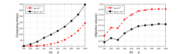
Figure 1: The computing time and objective value of Algorithm 1 due to Datta and Zou (2017) with the stopping condition $\max(\|A_{i+1}\!-A_{i}\|_{F},\|B_{i+1}\!-B_{i}\|,\|\Lambda_{i+1}\!-\Lambda_{i}\|)\leq{\rm tol}$

We also notice that a Dantzig selector type estimator and its improved version were proposed in (Rosenbaum and Tsybakov, 2010, 2013) and Belloni, Rosenbaum and Tsybakov (2017), respectively, for additive measurement error models. Since these estimators are defined via an optimization problem with an D.C. (difference of convexity) constraint, it is difficult to obtain these estimators in practice. To overcome the difficulty caused by the D.C. constraint, they recently relaxed the nonconvex constraint set to a convex set and proposed two conic programming based on estimators for the same model setup (see Belloni, Rosenbaum and Tsybakov (2016)), which can be viewed as a relaxed version of the Dantzig selector for the clean data. In addition, Städler and Bühlmann (2012) derived an algorithm for sparse linear regression with missing data based on a sparse inverse covariance matrix estimation. In the same spirit of Loh and Wainwright (2012) and Datta and Zou (2017), we propose the CaZnRLS estimator that can handle simultaneously additive errors, multiplicative errors and missing data case. Although the CaZnRLS estimator is defined by a nonconvex optimization problem, the GEP-MSCRA in Bi and Pan (2018) (see Section 3) provides an efficient solver for it, which consists of solving a sequence of weighted $\ell_{1}$-regularized LS problems. As shown by the simulation study in Section 5, the estimator still displays its merits in reducing prediction error and capturing sparsity for the contaminated data as it does for the clean data.

The rest of this paper is organized as follows. In Section 2, we define the calibrated zero-norm regularized LS estimator and provide a primal-dual view on this estimator. Section 3 describes the GEP-MSCRA solver for computing the CaZnRLS estimator. In Section 4, under a restricted eigenvalue assumption on the matrix $\Sigma$, we provide the deterministic theoretical guarantees including the $\ell_{2}$-error bound for every iterate, the decreasing of the error bound sequence, and the sign consistency of the iterates after finite steps; and the statistical guarantees for the computed estimator under two types of measurement errors. In Section 5, we compare the performance of CaZnRLS with that of CoCoLasso and NCL.

To close this section, we introduce some necessary notations. Let $\mathbb{S}^{p}$ be the space consisting of all $p\times p$ real symmetric matrices, equipped with the trace inner product $\langle W,Y\rangle={\rm trace}(W^{\mathbb{T}}Y)$ and its induced Frobenius norm $\|\cdot\|_{F}$, and let $\mathbb{S}_{+}^{p}$ be the cone consisting of all PSD matrices in $\mathbb{S}^{p}$. For any symmetric matrix $W$, let $\lambda_{\rm min}(W)$ and $\lambda_{\rm max}(W)$ denote the smallest and largest eigenvalues of $W$. For any vector $z$, $\|z\|_{\infty}$ denotes the infinity norm of $z$. Let $I$ and $e$ denote an identity matrix and a vector of all ones, respectively, whose dimensions are known from the context. For a closed set $\Omega$, $\delta_{\Omega}(\cdot)$ denotes the indicator function on $\Omega$, i.e., $\delta_{\Omega}(x)=0$ if $x\in\Omega$ and otherwise $\delta_{\Omega}(x)=+\infty$; and when $\Omega$ is convex, $\Pi_{\Omega}(\cdot)$ denotes the projection operator onto $\Omega$. For an index set $\Lambda\subseteq\{1,\ldots,p\}$, write $\Lambda^{c}:=\{1,\ldots,p\}\backslash\Lambda$ and denote by $\mathbb{I}_{\Lambda}(\cdot)$ the characterization function on $\Lambda$, and $Y_{\Lambda}$ by the submatrix of $Y$ consisting of the column $Y_{j}$ with $j\in\Lambda$. For any nonnegative real number $a$, $\lfloor a\rfloor$ and $\lceil a\rceil$ denote the largest integer less than $a$ and the smallest integer greater than $a$, respectively.

2 Calibrated zero-norm regularized LS estimator

When the data is corrupted by measurement errors, the observed matrix $Z$ of predictors is a function of the true covariate matrix $X$ and random errors. In this case, one may construct an unbiased surrogate $(\widehat{\Sigma},\widehat{\xi})$ for the pair $(\Sigma,\xi)$ with $Z$ and $y$ as in Loh and Wainwright (2012). For the specific form of $(\widehat{\Sigma},\widehat{\xi})$ under various types of measurement errors, one may refer to Section 2 in Loh and Wainwright (2012) or see Appendix B. Now assume that an unbiased surrogate $(\widehat{\Sigma},\widehat{\xi})$ is available. Let $\widehat{\Sigma}$ have the eigenvalue decomposition as $\widehat{\Sigma}=P{\rm Diag}(\theta_{1},\ldots,\theta_{p})P^{\mathbb{T}}$ where $P$ is a $p\times p$ orthonormal matrix and $\theta_{1}\geq\theta_{2}\geq\cdots\geq\theta_{p}$ are the eigenvalues of $\widehat{\Sigma}$.

Since it is time-consuming to compute a solution of (1.5) when $p$ is large, we replace the elementwise maximum norm in (1.5) with the Frobenius norm and achieve a nearest PD approximation to $\widehat{\Sigma}$ via the following model

$$\widetilde{\Sigma}=\mathop{\arg\min}_{W\succeq\widehat{\epsilon}I}\|W-\widehat{\Sigma}\|_{F}.$$ (2.1)

Note that (2.1) has the same solution set as $\min_{W\succeq\widehat{\epsilon}I}\|W-\widehat{\Sigma}\|_{F}^{2}$ does. So,

$$\widetilde{\Sigma}=\widehat{\epsilon}I+\Pi_{\mathbb{S}_{+}^{p}}(\widehat{\Sigma}\!-\!\widehat{\epsilon}I)=P{\rm Diag}\big{(}\max(\theta_{1},\widehat{\epsilon}),\ldots,\max(\theta_{p},\widehat{\epsilon})\big{)}P^{\mathbb{T}}.$$ (2.2)

Clearly, when $\widehat{\Sigma}=\frac{1}{n}Z^{\mathbb{T}}Z-\tau^{2}I$, a composite of a low-rank matrix and an identity matrix, the solution $\widetilde{\Sigma}$ keeps this structure. Also, one eigenvalue decomposition of $\frac{1}{n}Z^{\mathbb{T}}Z$ is enough to formulate the solution $\widetilde{\Sigma}$. Indeed, let

$$\left\{\begin{array}[]{ll}\widetilde{Z}:=\sqrt{n}P{\rm Diag}\Big{(}\sqrt{\max(\theta_{1},\widehat{\epsilon})},\ldots,\sqrt{\max(\theta_{p},\widehat{\epsilon})}\Big{)}P^{\mathbb{T}},\\ \widetilde{y}:=\sqrt{n}P{\rm Diag}\Big{(}\frac{1}{\sqrt{\max(\theta_{1},\widehat{\epsilon})}},\ldots,\frac{1}{\sqrt{\max(\theta_{p},\widehat{\epsilon})}}\Big{)}P^{\mathbb{T}}\widehat{\xi}.\end{array}\right.$$ (2.3)

By invoking (2.2), one may check that $\widetilde{\Sigma}=\frac{1}{n}\widetilde{Z}^{\mathbb{T}}\widetilde{Z}$ and $\widehat{\xi}=\frac{1}{n}\widetilde{Z}^{\mathbb{T}}\widetilde{y}$.

Although the computation of $\widetilde{\Sigma}$ becomes much cheaper than that of $\overline{\Sigma}$, it is a worse approximation to $\widehat{\Sigma}$ than the latter since the minimization of the elementwise maximum norm tends to give smaller entries. This requires us to define an estimator by more effective high-dimensional regression methods than Lasso. A natural candidate is the nonconvex type estimator such as SCAD and MCP since they can remove the bias of Lasso. Note that SCAD and MCP functions are actually imitating the performance of zero-norm. We define the zero-norm regularized LS estimator

$$\widetilde{\beta}\in\mathop{\arg\min}_{\beta\in\mathbb{R}^{p}}\Big{\{}\frac{1}{2n\lambda}\|\widetilde{Z}\beta-\widetilde{y}\|^{2}+\|\beta\|_{0}\Big{\}}.$$ (2.4)

Taking into account that $(\widetilde{Z},\widetilde{y})$ is a calibrated pair of $(\widehat{\Sigma},\widehat{\xi})$, we call (2.4) a calibrated version of the zero-norm regularized LS estimator defined with the corrupted observation $Z$ as in (1.2), except that the ball constraint is now removed due to the coerciveness of the strong convex $\|\widetilde{Z}\beta-\widetilde{y}\|^{2}$. Compared with the SCAD estimator, the solution of (2.4) seems to be much more difficult since the problem (2.4) is even discontinuous due to the combinatorial property of zero-norm. However, as demonstrated later, the SCAD estimator is actually equivalent to the zero-norm regularized LS.

Next we shall provide a primal-dual look into the estimator $\widetilde{\beta}$. Define

$$\phi(t):=\frac{a\!-\!1}{a\!+\!1}t^{2}+\frac{2}{a\!+\!1}t\ \ (a>1)\quad\ {\rm for}\ \ t\in\mathbb{R}.$$ (2.5)

With this function, it is immediate to check that for any $\beta\in\mathbb{R}^{p}$,

$$\|\beta\|_{0}=\min_{w\in\mathbb{R}^{p}}\!\bigg{\{}\sum_{i=1}^{p}\phi(w_{i})\!:\langle e-w,|\beta|\rangle=0,\ 0\leq w\leq e\bigg{\}}.$$

This shows that the zero-norm is essentially an optimal value function of a parameterized MPEC, since $\langle e-w,|\beta|\rangle=0$ and $e-w\geq 0$ constitute an equilibrium constraint. Thus, (2.4) is equivalent to the following MPEC

$$\min_{\beta,w\in\mathbb{R}^{p}}\!\bigg{\{}\frac{1}{2n\lambda}\|\widetilde{Z}\beta-\widetilde{y}\|^{2}+\sum_{i=1}^{p}\phi(w_{i})\!:\,\langle e-w,|\beta|\rangle=0,\,0\leq w\leq e\bigg{\}},$$ (2.6)

in the sense that if $\widetilde{\beta}^{\natural}$ is a global optimal solution of (2.4), then $(\widetilde{\beta}^{\natural},{\rm sign}(|\widetilde{\beta}^{\natural}|))$ is globally optimal to (2.6); and conversely, if $(\widetilde{\beta}^{\natural},\widetilde{w}^{\natural})$ is a global optimal solution of (2.6), then $\widetilde{\beta}^{\natural}$ is globally optimal to (2.4) with $\|\widetilde{\beta}^{\natural}\|_{0}=\sum_{i=1}^{p}\phi(\widetilde{\beta}^{\natural}_{i})$.

The MPEC form (2.6) shows that the difficulty to compute the estimator $\widetilde{\beta}$ arises from the constraint $\langle e-\!w,|\beta|\rangle=0$, which brings the bothersome nonconvexity. Since it is much harder to handle nonconvex constraints than to handle nonconvex objective, we consider its penalized version

$$\min_{\beta\in\mathbb{R}^{p},w\in[0,e]}\!\bigg{\{}\frac{1}{2n\lambda}\|\widetilde{Z}\beta-\widetilde{y}\|^{2}+\sum_{i=1}^{p}\phi(w_{i})+\rho\langle e-w,|\beta|\rangle\bigg{\}}$$ (2.7)

where $\rho>0$ is the penalty parameter. By the coerciveness of the function $\beta\mapsto\|\widetilde{Z}\beta-\widetilde{y}\|^{2}$, there exists a constant $\widehat{R}>0$ such that (2.6) and (2.7) are equivalent to their respective version in which the variable $\beta$ is required to lie in the set $\{\beta\in\mathbb{R}^{p}\ |\ \|\beta\|_{\infty}\leq\widehat{R}\}$. Thus, by invoking Theorem 2.1 of Bi and Pan (2018), we have the following result.

Theorem 1.

Let $L_{\!f}$ be the Lipschitz constant of $f(\beta):=\frac{1}{2n}\|\widetilde{Z}\beta-\widetilde{y}\|^{2}$ on the ball $\{\beta\in\mathbb{R}^{p}\!:\|\beta\|_{\infty}\leq\widehat{R}\}$. Then, for every $\rho\geq\overline{\rho}:=\frac{4aL_{\!f}}{(a+1)\lambda}$, the global optimal solution set of (2.7) associated to $\rho$ coincides with that of (2.6).

Theorem 1 shows that the problem (2.7) is a global exact penalty of (2.6) in the sense that it has the same global optimal solution set as (2.6) does once $\rho$ is greater than a threshold. Consequently, the estimator $\widetilde{\beta}$ can be achieved by solving the following exact penalty problem with $\rho>\overline{\rho}$:

$$\widetilde{\beta}\in\mathop{\arg\min}_{\beta\in\mathbb{R}^{p},w\in[0,e]}\!\bigg{\{}\frac{1}{2n}\|\widetilde{Z}\beta-\widetilde{y}\|^{2}+\sum_{i=1}^{p}\lambda\Big{[}\phi(w_{i})+\rho(1-w_{i})|\beta_{i}|\Big{]}\bigg{\}}.$$ (2.8)

Compared with (2.4), the problem (2.8) involves an additional variable $w\in\mathbb{R}^{p}$ which provides a part of dual information on (2.4). Hence, (2.8) can be viewed as a primal-dual equivalent form of (2.4). This form does not involve the combinatorial difficulty, and its nonconvexity is just due to the coupled term $\langle w,|\beta|\rangle$ which is clearly much easier to cope with. In particular, the SCAD function in Fan and Li (2001) is precisely the optimal value of the inner minimization in (2.8) w.r.t. $w$. To see this, we define

$$\psi(t):=\!\left\{\!\begin{array}[]{cl}\phi(t)&\textrm{if}\ t\in[0,1],\\ +\infty&\textrm{otherwise}.\end{array}\right.$$ (2.9)

Recalling the conjugate $\psi^{*}(\omega)=\sup_{t\in\mathbb{R}}\{t\omega-\psi(t)\}$ of $\psi$ by Rockafellar (1970), we can compactly write the inner minimization in (2.8) w.r.t. $w$ as

$$\min_{w\in\mathbb{R}^{p}}\!\Big{\{}{\textstyle\sum_{i=1}^{p}}\lambda\big{[}\psi(w_{i})+\rho(1\!-\!w_{i})|\beta_{i}|\big{]}\Big{\}}={\textstyle\sum_{i=1}^{p}}\lambda\big{[}\rho|\beta_{i}|-\psi^{*}\big{(}\rho|\beta_{i}|\big{)}\big{]}.$$

After an elementary calculation, the conjugate $\psi^{*}$ of $\psi$ has the form of

$$\psi^{*}(\omega)=\left\{\!\begin{array}[]{cl}0&\textrm{if}\ \omega\leq\frac{2}{a+1},\\ \frac{((a+1)\omega-2)^{2}}{4(a^{2}-1)}&\textrm{if}\ \frac{2}{a+1}<\omega\leq\frac{2a}{a+1},\\ \omega-1&\textrm{if}\ \omega>\frac{2a}{a+1}.\end{array}\right.$$

By comparing with the expression of the SCAD function $p_{\gamma}(t)$, the function $\lambda[\rho|t|-\psi^{*}(\rho|t|)]$ with $\lambda=\frac{(a+1)\gamma^{2}}{2}$ and $\rho=\frac{2}{(a+1)\gamma}$ reduces to $p_{\gamma}(t)$. Thus,

$$\widetilde{\beta}\in\mathop{\arg\min}_{\beta\in\mathbb{R}^{p}}\!\Big{\{}\frac{1}{2n}\|\widetilde{Z}\beta-\widetilde{y}\|^{2}+{\textstyle\sum_{i=1}^{p}}p_{\gamma}(|\beta_{i}|)\Big{\}}.$$ (2.10)

3 GEP-MSCRA for computing the estimator $\widetilde{\beta}$

From the last section, to compute the estimator $\widetilde{\beta}$, one only needs to solve a single penalty problem (2.8) which is much easier than (2.4) since its nonconvexity is from the coupled term $\langle w,|\beta|\rangle$. The GEP-MSCRA proposed in Bi and Pan (2018) makes good use of the coupled structure and solves the problem (2.8) in an alternating way. Since the threshold $\overline{\rho}$ is unknown though one may obtain an upper estimation for it, a varying $\rho$ is introduced in GEP-MSCRA. The iterations of GEP-MSCRA are described below.

Algorithm 1   GEP-MSCRA for computing $\widetilde{\beta}$

Initialization: Choose $\lambda>0,\rho_{0}=1$ and an initial $w^{0}\in[0,\frac{1}{2}e]$. Set $k:=1$.
while the stopping conditions are not satisfied do

1. Compute the following minimization problem

   $$\beta^{k}=\mathop{\arg\min}_{\beta\in\mathbb{R}^{p}}\bigg{\{}\frac{1}{2n}\big{\|}\widetilde{Z}\beta-\widetilde{y}\big{\|}^{2}+\lambda\sum_{i=1}^{p}(1\!-\!w_{i}^{k-1})|\beta_{i}|\bigg{\}}.$$ (3.1)

2. When $k=1$, select a suitable $\rho_{1}\geq\rho_{0}$ in terms of $\|\beta^{1}\|_{\infty}$. Otherwise, select $\rho_{k}$ such that $\rho_{k}\geq\rho_{k-1}$ for $k\leq 3$; and $\rho_{k}=\rho_{k-1}$ for $k>3$.

3. Seek the unique optimal solution $w_{i}^{k}\ (i=1,\ldots,p)$ of the problem

   $$w_{i}^{k}=\mathop{\rm arg\min}_{0\leq w_{i}\leq 1}\left\{\phi(w_{i})-\rho_{k}w_{i}|\beta^{k}_{i}|\right\}.$$ (3.2)

4. Let $k\leftarrow k+1$, and then go to Step 1.

end while

Remark 1.

(a) Since $\phi$ is strongly convex, the problem (3.2) has a unique optimal solution. By the expression of $\phi$, it is immediate to obtain

$$w_{i}^{k}=\min\Big{[}1,\max\Big{(}\frac{(a+1)\rho_{k}|\beta^{k}_{i}|-2}{2(a-1)},0\Big{)}\Big{]}\ \ {\rm for}\ \ i=1,2,\ldots,p.$$ (3.3)

Thus, the main computation work of GEP-MSCRA in each step is solving a weighted $\ell_{1}$-regularized LS. In this sense, GEP-MSCRA is analogous to the local linear approximation algorithm Zou and Li (2008) applied to the problem (2.10) except the start-up and the weights, where the start-up of the former depends explicitly on the dual variable $w^{0}$, while that of the latter depends implicitly on a good estimator $\beta^{0}$. So, when computing CaZnRLS with GEP-MSCRA, one actually obtains an adaptive Lasso estimator. The initial $w^{0}$ may be an arbitrary vector from the box set $[0,\frac{1}{2}e]$. Here, we restrict $w^{0}$ to the box set $[0,\frac{1}{2}e]$, rather than the feasible set $[0,e]$ of $w$ in (2.8), so as to achieve a better initial estimator $\beta^{1}$.

(b) Due to the combinatorial property of $\|\cdot\|_{0}$, it is almost impossible to get $\widetilde{\beta}$ exactly. The popular Lasso of Tibshirani (1996) or adaptive Lasso of Zou (2006), as a one-step or series of convex relaxation to (2.4), arises from the primal angle, while the series of weighted $\ell_{1}$-norm regularized LS problems in GEP-MSCRA arise from the primal-dual reformulation of (2.4).

(c) From the formula (3.3), if $\rho_{k}|\beta^{k}_{i}|$ is larger, then $w_{i}^{k}$ has a value close to $1$, which means that in the $(k\!+\!1)$th iterate, a smaller weight $(1\!-\!w_{i}^{k})$ is imposed on the variable $\beta_{i}$, and consequently a conservative strategy is used for sparsity. Consider that for some difficult problems, the solution $\beta^{1}$ yielded by the $\ell_{1}$-regularized LS problem may not have a sharp gap between its nonzero and zero entries. Hence, in order to guarantee that the subsequent $\beta^{k}$ has a correct sparse support, we increase $\rho_{k}$ for $k\leq 3$ appropriately, i.e., cut down the smaller nonzero entries conservatively, while for $k>3$ since $\beta^{k}$ generally has a big difference between its nonzero and zero entries, we keep $\rho_{k}$ unchanged so as to cut down the smaller nonzero entries quickly.

In Appendix C, we provide the implementation details of GEP-MSCRA with the semismooth Newton augmented Lagrangian method (ALM) applied to the dual of (3.1). As discussed in Li, Sun and Toh (2018), the semismooth Newton ALM fully exploits the second-order information of and the good structure of its dual and can yield a solution of high accuracy.

4 Theoretical guarantees for the GEP-MSCRA

In this section we denote by $S^{*}$ the support of the true vector $\beta^{*}$, and define

$$\mathcal{C}(S^{*}):=\bigcup_{S\supset S^{*},|S|\leq 1.5s}\!\Big{\{}\beta\in\mathbb{R}^{p}\!:\|\beta_{S^{c}}\|_{1}\leq 3\|\beta_{S}\|_{1}\Big{\}}.$$

We say that $\Sigma$ satisfies the $\kappa$-restricted eigenvalue condition (REC) or $X$ satisfies the $\kappa$-restricted strong convexity on $\mathcal{C}(S^{*})$ if $\kappa>0$ is such that

$$\beta^{\mathbb{T}}\Sigma\beta=\frac{1}{n}\|X\beta\|^{2}\geq\kappa\|\beta\|^{2}\quad{\rm for\ all}\ \beta\in\mathcal{C}(S^{*}).$$

This REC is a little stronger than the one used in Negahban et al. (2012) for the clean Lasso and in Datta and Zou (2017) for CoCoLasso since $\mathcal{C}(S^{*})\supseteq\big{\{}\beta\in\mathbb{R}^{p}\!:\|\beta_{(S^{*})^{c}}\|_{1}\leq 3\|\beta_{S^{*}}\|_{1}\big{\}}$, and is different from the $(L,S^{*},N)$-restricted eigenvalue condition introduced in van de Geer and Bühlmann (2009). We shall provide the deterministic theoretical guarantees for GEP-MSCRA under this REC with appropriate $\lambda,\rho_{1}$ and $\rho_{3}$, which include the error bound of every iterate $\beta^{k}$ to the true $\beta^{*}$, the decrease analysis of the error sequence, and the sign consistency analysis of $\beta^{k}$ after finite steps. All proofs of the main results are included in Appendix A.

4.1. Error bound sequence and its decrease

To achieve the error bound of the iterate $\beta^{k}$ to the true $\beta^{*}$, we write

$$D:=\widehat{\Sigma}-\Sigma\ \ {\rm and}\ \ \widetilde{\varepsilon}:=\widehat{\xi}-\widetilde{\Sigma}\beta^{*}.$$ (4.4)

The following theorem states a deterministic result for the error bound.

Theorem 2.

Suppose $\Sigma$ satisfies the $\kappa$-REC on $\mathcal{C}(S^{*})$ with $\kappa>24s\|D\|_{\rm max}$. If $\lambda$ and $\rho_{3}$ are chosen with $\lambda\geq 8\|\widetilde{\varepsilon}\|_{\infty}$ and $\rho_{3}\leq\frac{2(\kappa-24s\|D\|_{\rm max})}{5\sqrt{2}\lambda}$, then

$$\|\beta^{k}-\beta^{*}\|\leq\frac{5\sqrt{s}\,\lambda}{2(\kappa-24s\|D\|_{\rm max})}\quad\ \forall k\in\mathbb{N}.$$ (4.5)

The error bound in Theorem 2 has the same order, i.e. $O(\lambda\sqrt{s})$, as established for the clean Lasso in Negahban et al. (2012). From the proof of Theorem 1 in Datta and Zou (2017), $\|D\|_{\rm max}\leq\frac{\kappa}{64s}$ holds with a high probability. This means that there is a high probability for the error bound of $\beta^{k}$ not greater than $\frac{4\lambda\sqrt{s}}{\kappa}$, which is a little better than the bound $\frac{4\sqrt{2}\lambda\sqrt{s}}{\kappa}$ in Datta and Zou (2017) although $\lambda$ is allowed to be greater than $8\|\widetilde{\varepsilon}\|_{\rm\infty}$ instead of $2\|\widetilde{\varepsilon}\|_{\infty}$ as in Datta and Zou (2017).

Theorem 2 provides an error bound for every iterate, but it does not tell us if the error bound of the current $\beta^{k}$ is better than that of the previous $\beta^{k-1}$. To seek the answer, we study the decrease of the error bound sequence by bounding $(1\!-\!w^{k}_{i})^{2}$ for $i\in S^{*}$. Write $F^{0}:=S^{*}$ and for $k\in\mathbb{N}$ define

$$F^{k}:=\Big{\{}i\!:\big{|}|\beta_{i}^{k}|-|\beta_{i}^{*}|\big{|}\geq(\rho_{k})^{-1}\Big{\}}\ {\rm and}\ \Lambda^{k}:=\Big{\{}i\!:|\beta_{i}^{*}|\leq\frac{4a}{(a\!+\!1)\rho_{k}}\Big{\}}.$$ (4.6)

By Lemma 3, $(1\!-w^{k}_{i})^{2}$ for $i\in S^{*}$ can be controlled by $\max(\mathbb{I}_{\Lambda^{k}}(i),\mathbb{I}_{F^{k}}(i))$. As a consequence, we have the following error bound result involving $\mathbb{I}_{\Lambda^{k}}(i)$.

Theorem 3.

Suppose $\Sigma$ satisfies the $\kappa$-REC on $\mathcal{C}(S^{*})$ with $\kappa>24s\|D\|_{\rm max}$. If $\lambda$ and $\rho_{3}$ are chosen in the same way as in Theorem 2, then

$$\big{\|}\beta^{k}\!-\beta^{*}\big{\|} \leq\frac{4+2\sqrt{2}}{\kappa-24s\|D\|_{\rm max}}\big{\|}\widetilde{\varepsilon}_{\!S^{*}}\big{\|}+\Big{(}\frac{1}{\sqrt{2}}\Big{)}^{k-1}\big{\|}\beta^{1}\!-\beta^{*}\big{\|}$$

$$\quad+\frac{2\lambda}{\kappa-24s\|D\|_{\rm max}}\sum_{j=1}^{k-1}\!\sqrt{{\textstyle\sum_{i\in S^{*}}}\mathbb{I}_{\Lambda^{j}}(i)}\Big{(}\frac{1}{\sqrt{2}}\Big{)}^{k-1-j}\quad\forall k\in\mathbb{N}.$$

The error bound in Theorem 3 consists of three parts: statistical error $\|\widetilde{\varepsilon}_{\!S^{*}}\|$ induced by noise, the identification error $\sum_{j=1}^{k-1}\!\sqrt{{\textstyle\sum_{i\in S^{*}}}\mathbb{I}_{\Lambda^{j}}(i)}(\frac{1}{\sqrt{2}})^{k-1-j}$ related to the choice of $\rho_{j}$, and the computation error $(\frac{1}{\sqrt{2}})^{k-1}\|\beta^{1}\!-\beta^{*}\|$. By the definition of $\Lambda^{j}$, if $\rho_{j}$ is chosen such that $\rho_{j}>\frac{4a}{(a+1)\min_{i\in S^{*}}\!|\beta_{i}^{*}|}$, then the identification error becomes zero, and consequently the error bound sequence will decrease to the statistical error $\|\widetilde{\varepsilon}_{\!S^{*}}\|$ as $k$ increases. Clearly, if $\min_{i\in S^{*}}\!|\beta_{i}^{*}|$ is not too small, it is easy to choose such $\rho_{j}$. In the next part, we shall provide an explicit choice range of $\rho_{j}$ such that the identification error is zero. From Theorem 3, we also observe that a smaller error bound of $\beta^{1}$ brings a smaller error bound for $\beta^{k}$ with $k\geq 2$. The importance of $\beta^{1}$ also comes from the fact that one may use it to estimate the choice range of $\rho_{j}\ (j\geq 1)$ since $\|\widetilde{\varepsilon}\|_{\infty}$ is unknown in practice. During the implementation of GEP-MSCRA, we choose $\rho_{1}$ according to this strategy.

4.2. Sign consistency

We show that if the smallest nonzero component of $\beta^{*}$ is not so small, GEP-MSCRA can deliver $\beta^{l}$ satisfying ${\rm supp}(\beta^{l})={\rm supp}(\beta^{*})$ within finite steps. To achieve this goal, we need the oracle least squares solution:

$$\beta^{{\rm LS}}\in\mathop{\arg\min}_{\beta\in\mathbb{R}^{p}}\left\{\frac{1}{2n}\|\widetilde{Z}\beta-\widetilde{y}\|^{2}:\ {\rm supp}(\beta)\subseteq S^{*}\right\}.$$ (4.7)

Write $\varepsilon^{{\rm LS}}:=\frac{1}{n}\widetilde{Z}^{\mathbb{T}}(\widetilde{y}-\widetilde{Z}\beta^{\rm LS})$. Then $\varepsilon_{S^{*}}^{{\rm LS}}=\widetilde{Z}_{\!S^{*}}^{\mathbb{T}}(\widetilde{Z}\beta^{{\rm LS}}-\widetilde{y})=0.$ This implies that $\beta^{\rm LS}_{S^{*}}-\beta^{*}_{S^{*}}=\widetilde{\Sigma}_{\!S^{*}S^{*}}^{-1}\big{[}\frac{1}{n}\widetilde{Z}^{\mathbb{T}}_{\!S^{*}}\big{(}\widetilde{Z}\beta^{\rm LS}-\widetilde{Z}\beta^{*}\big{)}\big{]}=\widetilde{\Sigma}_{\!S^{*}S^{*}}^{-1}\big{[}\frac{1}{n}\widetilde{Z}^{\mathbb{T}}_{S^{*}}(\widetilde{y}-\widetilde{Z}\beta^{*})\big{]},$ and

$$\beta^{\rm LS}_{S^{*}}-\beta^{*}_{S^{*}}=\widetilde{\Sigma}_{\!S^{*}S^{*}}^{-1}\big{(}\widehat{\xi}_{S^{*}}-\widetilde{\Sigma}_{\!S^{*}S^{*}}\beta^{*}_{S^{*}}\big{)}=\widetilde{\Sigma}_{\!S^{*}S^{*}}^{-1}\widetilde{\varepsilon}_{\!S^{*}}:=\widetilde{\varepsilon}^{\dagger}.$$ (4.8)

Based on this observation for $\beta^{\rm LS}$, we can establish the following result.

Theorem 4.

Suppose $\Sigma$ satisfies the $\kappa$-REC on $\mathcal{C}(S^{*})$ with $\kappa>24s\|D\|_{\rm max}$. Set $\gamma:=\kappa-24s\|D\|_{\rm max}$. If $\lambda,\rho_{1}$ and $\rho_{3}$ are chosen with $\lambda\geq 6\|\varepsilon^{\rm LS}\|_{\infty}$, $\rho_{1}\!>\!\max\!\big{(}\frac{4a}{(a+1)\min_{i\in S^{*}}\!|\beta^{*}_{i}\!|},\gamma\lambda^{-1}\|\widetilde{\varepsilon}^{\dagger}\|_{\infty}\big{)}$ and $\rho_{3}\leq\!\sqrt{\frac{4\gamma}{9\sqrt{3}\lambda}}$, then for all $k\in\mathbb{N}$

$$\big{\|}\beta^{k}-\beta^{\rm{LS}}\big{\|}\leq\frac{2.03\rho_{k-1}\lambda}{\gamma}\sqrt{|F^{k-1}|},\,\sqrt{|F^{k}|}\leq\frac{18.27\sqrt{3}\rho_{k}\rho_{k-1}\lambda}{(9\sqrt{3}\!-\!4)\gamma}\sqrt{|F^{k-1}|}.$$

In particular, when $k\geq\overline{k}$ with $\overline{k}=\big{\lceil}\frac{0.5\ln(s)}{\ln[(9\sqrt{3}\!-\!4)\gamma\lambda^{-1}]-\ln[18.27\sqrt{3}(\rho_{3})^{2}]}\big{\rceil}$, we have

$$\beta^{k}=\beta^{\rm LS}\ \ {\rm and}\ \ {\rm sign}(\beta^{k})={\rm sign}(\beta^{*}).$$

Remark 2.

(a) Notice that Datta and Zou (2017) achieved the sign consistency of $\overline{\beta}$ under an irrepresentable condition on $\Sigma$ and the condition $\min_{i\in S^{*}}\!|\beta^{*}_{i}\!|>\![4\|\Sigma_{S^{*}S^{*}}^{-1}\|_{\infty}+(\lambda_{\min}(\Sigma_{S^{*}S^{*}}))^{-1/2}]\lambda$, where $\|A\|_{\infty}=\max_{i}\sum_{j}|A_{ij}|$ means the matrix $\ell_{\infty}$-norm. Their irrepresentable condition on $\Sigma$ requires that $\|\Sigma_{(S^{*})^{c}S^{*}}\Sigma_{S^{*}S^{*}}^{-1}\|_{\infty}\!\leq\overline{\gamma}<1$ and $\lambda_{\rm min}(\Sigma_{S^{*}S^{*}})\geq\!C_{\rm min}$ for some constants $\overline{\gamma}>0$ and $C_{\rm min}\!>0$, in which the former makes a restriction on the scale of the entries of $\Sigma$ and the latter is precisely the REC of $\Sigma$ on the set $\big{\{}\beta\in\mathbb{R}^{p}\!:\beta_{(S^{*})^{c}}=0\big{\}}$. We obtain the sign consistency of $\beta^{k}$ for $k\geq\overline{k}$ under the $\kappa$-REC of $\Sigma$ on $\mathcal{C}(S^{*})$ with $\kappa>24s\|D\|_{\rm max}$ and $\rho_{1}\!>\!\max\!\big{(}\frac{4a}{(a+1)\min_{i\in S^{*}}\!|\beta^{*}_{i}\!|},\gamma\lambda^{-1}\|\widetilde{\varepsilon}^{\dagger}\|_{\infty}\big{)}$. When $\lambda_{\rm min}(\Sigma_{S^{*}S^{*}})$ is large, there is a great possibility for our $\kappa$-REC to hold. Also, when $\|\Sigma_{(S^{*})^{c}S^{*}}\Sigma_{S^{*}S^{*}}^{-1}\|_{\infty}\leq\overline{\gamma}$ does not hold, our $\kappa$-REC may hold; for example, consider $\Sigma=[1\ 0\ 2;0\ 1\ 2;2\ 2\ 9]$ and $S^{*}=\{1,2\}$. In fact, to some extent, our $\kappa$-REC also depends on the unbiased surrogate $\widehat{\Sigma}$ of $\Sigma$. If $\|\widehat{\Sigma}-\Sigma\|_{\rm max}$ is small, there is a great possibility for our $\kappa$-REC to hold. Finally, the condition on $\min_{i\in S^{*}}\!|\beta^{*}_{i}\!|$ used by Datta and Zou (2017) implies a large choice range for our parameter $\rho_{1}$ whether $\|\Sigma_{S^{*}S^{*}}^{-1}\|_{\infty}$ or $(\lambda_{\min}(\Sigma_{S^{*}S^{*}}))^{-1/2}$ is larger or $\lambda$ is larger.

(b) Notice that $\rho_{3}\leq\!\sqrt{\frac{4\gamma}{9\sqrt{3}\lambda}}$. Together with the definition of $\overline{k}$, we have $\ln[(9\sqrt{3}\!-\!4)\gamma\lambda^{-1}]-\ln[18.27\sqrt{3}(\rho_{3})^{2}]\geq\ln(1.4)$, which with $s\geq 9$ implies that $\overline{k}\leq\widehat{k}:=\big{\lceil}\frac{0.5\ln(s)}{\ln(1.4)}\big{\rceil}.$ As one referee pointed out that $\overline{k}$ or $\widehat{k}$ is actually unknown since it depends on the sparsity $s$ of $\beta^{*}$. In practice, some prior upper estimation on $s$ is available; for example, a rough upper estimation on $s$ is the dimension $p$. Thus, one still can obtain a rough upper estimation on $\widehat{k}$. In the practical numerical computation, one can identify such $\overline{k}$ by monitoring the index change of nonzero entries in each iterate.

(c) By Theorem 4, the choice of $\rho_{1}$ is crucial for GEP-MSCRA to yield an oracle solution whose sign is consistent with that of $\beta^{*}$ after finite steps. As remarked after Theorem 3, whether such $\rho_{1}$ is easily chosen or not depends on the error bound of $\beta^{1}$. From Theorem 4 and Theorem 3, we conclude that a smaller $\rho_{3}$ entails a good output of GEP-MSCRA in terms of the error bound and sign consistency, and for those problems with high noise, a large $\lambda$ is needed, and of course the error bound of $\beta^{k}$ becomes large.

We have established the deterministic theoretical guarantees of GEP-MSCRA for computing the calibrated zero-norm regularized LS estimator under suitable conditions. From (Raskutti, Wainwright and Yu, 2010, 2011), if $X$ is from the $\Sigma_{x}$-Gaussian ensemble (i.e., $X$ is formed by independently sampling each row $X^{i}\sim N(0,\Sigma_{x})$, there exists a constant $\kappa>0$ (depending on $\Sigma_{x}$) such that $\Sigma$ satisfies the REC on $\mathcal{C}(S^{*})$ with probability greater than $1\!-\!c_{1}\exp(-c_{2}n)$ as long as $n>cs\ln p$, where $c,c_{1}$ and $c_{2}$ are absolutely positive constants. It is natural to ask whether such $\kappa$ satisfies the requirement of the above theorems or not. Is there a big possibility to choose $\lambda,\rho_{1}$ and $\rho_{3}$ as required in the above theorems? In Appendix B, we focus on these questions for two specific types of errors-in-variables models.

5 Numerical experiments

We use simulated datasets to evaluate the performance of the CaZnRLS estimator, computed with GEP-MSCRA (see Appendix C for its implementation details), and compare its performance with that of CoCoLasso and NCL in terms of the number of signs identified correctly (NC) and identified incorrectly (NIC) for predictors, and the relative root-mean-square-error (RMSE). Let $\beta^{f}$ be the final output of one of three solvers. Define

$${\rm NC}(\beta^{f}):=\!\sum_{i\in S^{*}}\mathbb{I}\big{\{}|{\rm sign}(\beta_{i}^{f})-{\rm sign}(\beta_{i}^{*})|=0\big{\}},\qquad\qquad$$

$${\rm NIC}(\beta^{f}):=N_{\rm nz}(\beta^{f})-{\rm NC}(\beta^{f})\ \ {\rm and}\ \ {\rm relative\ RMSE}:=\frac{\|\beta^{f}-\beta^{*}\|}{\|\beta^{*}\|}$$

where $N_{\rm nz}(\beta^{f})\!:=\!\sum_{i=1}^{p}\mathbb{I}\big{\{}|\beta_{i}|>\!10^{-8}\big{\}}$ is the number of nonzero entries of $\beta^{f}$. All results are obtained in a desktop computer running on 64-bit Windows with an Intel(R) Core(TM) i7-7700 CPU 3.6GHz and 16 GB memory.

For GEP-MSCRA, we choose $a=6.0$ for $\phi$, $w^{0}=0$ and $\rho_{k}$ for $k\leq 3$ by

$$\rho_{1}=\max\Big{(}1,\frac{5}{3\|\beta^{1}\|_{\infty}}\Big{)},\ \rho_{k}=\min\Big{(}2\rho_{k-1},\frac{10^{8}}{\|\beta^{k}\|_{\infty}}\Big{)}\ {\rm for}\ k=2,3.$$

We terminate GEP-MSCRA at $\beta^{k}$ once the following condition is satisfied

$$\left\{\begin{array}[]{c}|N_{\rm nz}(\beta^{k-j})-N_{\rm nz}(\beta^{k-j-1})|\leq 5,\ j=0,1,2;\\ \big{|}\frac{1}{2n}\|\widetilde{Z}\beta^{k}\!-\!\widetilde{y}\|^{2}-\frac{1}{2n}\|\widetilde{Z}\beta^{k-1}\!-\!\widetilde{y}\|^{2}\big{|}\leq 0.1,\end{array}\right.$$

or the number of iterates is over the maximum number $k_{\rm max}=4$ (Our code can be achieved from https://github.com/SCUT-OptGroup/ErrorInvar). Such a stopping criterion aims to capture a solution $\beta^{k}$ whose sparsity tends to be stable on one hand, and on the other hand its predictor error has a small variation. In addition, by Remark 2(b), we have a rough upper estimation for $\overline{k}$ is $\lceil\frac{0.5\ln(p)}{\ln(1.4)}\rceil$, which equals $11$ for $p=1000$. In view of this, we set the maximum number of iterate to be $4$. We solve the dual of (3.1) with Algorithm 2 for $\epsilon^{j}=10^{-8}$. For NCL, we directly run the code “doProjGrad”, which is solving the model (1.4) with $\lambda_{n}=0$ and $R_{0}=\|\beta^{*}\|_{1}$, for the test examples. Since the Matlab code of CoCoLasso is not available, we include our implementation in Appendix D. Since it is time-consuming for Algorithm 4 to use the stopping rule $\max\{\epsilon_{{\rm pinf}}^{k},\epsilon_{{\rm dinf}}^{k},\epsilon_{{\rm gap}}^{k}\}\!\leq 10^{-5}$, we use the looser $\max\{\epsilon_{{\rm pinf}}^{k},\epsilon_{{\rm dinf}}^{k},10^{-3}\epsilon_{{\rm gap}}^{k}\}\!\leq 10^{-4}$ to get an approximate solution of (1.5), and then use Algorithm 2 to solve the associated problem (1.6).

From the theoretic results in Section 4, the appropriate $\lambda$ lies in an interval associated to $\|\widetilde{\varepsilon}\|_{\infty}$. Such $\lambda$ is also suitable for CoCoLasso by the proof of Theorem 1 and 2 in Datta and Zou (2017). In view of this, we set $\lambda=\max(0.01,\frac{\alpha^{*}}{n}\|\widetilde{Z}^{\mathbb{T}}\widetilde{y}\|_{\infty})$ and $\max(0.01,\frac{\alpha^{*}}{n}\|\overline{Z}^{\mathbb{T}}\overline{y}\|_{\infty})$ for CaZnRLS and CoCoLasso, respectively, where the appropriate $\alpha^{*}\in[0.06,0.32]$ is chosen by using $5$-fold corrected cross-validation proposed in Datta and Zou (2017).

Throughout this section, all test examples are generated randomly with the triple $(p,s,n)$ consisting of the dimension $p$ of predicted variable, the number of nonzero entries of $\beta^{*}$, and the sample size $n$. Among others, $n=\lfloor\alpha s\ln(p)\rfloor$ with $\alpha=4+0.2(j\!-\!1)$ for $j=1,\ldots,11$. We obtain the observation $y$ from the model (1.1) where the entries of $\varepsilon$ are i.i.d. $\mathcal{N}(0,\sigma^{2})$, and the generating way of the true $\beta_{S^{*}}^{*}$ is specified in the sequel. The average relative RMSE (respectively, NC and NIC) is the average of the total RMSE (respectively, NC and NIC) for $100$ problems generated randomly.

5.1. Random locations of the nonzero entries of $\beta^{*}$

In this part, we evaluate the performance of CaZnRLS by the examples generated randomly, where $\beta_{S^{*}}^{*}$ is an i.i.d. standard normal random vector with the $s=\lfloor 0.5\sqrt{p}\rfloor$ entries of $S^{*}$ chosen randomly from $\{1,\ldots,p\}$. First, we test whether CaZnRLS is stable with respect to the variance $\sigma$ of $\varepsilon$. 5.1.1. Performance of CaZnRLS under low and high noise

Example 1.

We generate $Z=X\!+A$ with $p=500$, where the rows of $X$ are i.i.d. standard normal random vectors with mean zero and covariance matrix $\Sigma_{X}=I$, and the rows of $A$ are i.i.d. $\mathcal{N}(0,I)$.

Figure 2 plots the average relative RMSE, NC and NIC curves of CaZnRLS, CoCoLasso and NCL for Example 1 under different sample sizes with $\sigma=0.5$ and $1.0$. The subfigures on the first column show that CaZnRLS is comparable even a little better than CoCoLasso in terms of the relative RMSE, the second column shows that the NC of CaZnRLS is at most $2$ fewer than that of CoCoLasso, while the third column indicates that the NIC of CaZnRLS is much fewer than that of CoCoLasso. From this, we conclude that CaZnRLS keeps the merit of the zero-norm regularized LS estimator in the clean data setting. We also see that CaZnRLS has a similar performance for $\sigma=0.5$ and $\sigma=1$, indicating that it is insensitive to the variance $\sigma$ of regression error. So, in the sequel we always take $\sigma=0.5$.

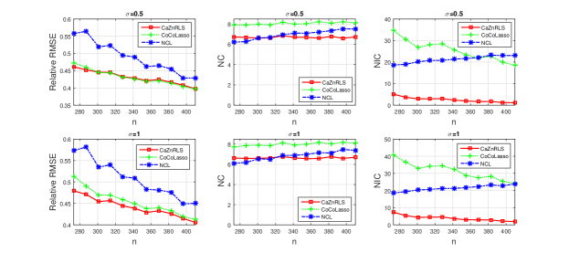
Figure 2: The relative RMSE, NC and NIC of three solvers under different $\sigma$

5.1.2. Performance of CaZnRLS for different measurement errors

In this part we evaluate the performance of CaZnRLS for three classes of measurement errors by using test problems generated with $p=1000$.

Case 1. Additive errors

Example 2.

We generate $Z=X+A$ where $X$ is same as in Example 1, and the rows of $A$ are i.i.d. $\mathcal{N}(0,\tau^{2}I)$ with $\tau=0.5$ or $1.0$.

Example 3.

We generate $Z=X+A$ where the entries of $X$ are i.i.d. and follow the uniform distribution on $(0,1)$, and $A$ is same as in Example 2.

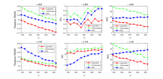
Figure 3: The relative RMSE, NC and NIC of three solvers under different $n$

Figure 3 plots the average relative RMSE, NC and NIC curves of three solvers under different sample sizes for Example 2. From this figure, whether $X$ is corrupted by high noise or low noise, CaZnRLS is the best among three solvers in terms of the relative RMSE and NIC, though its NC is (at most $1$) fewer than the NC of CoCoLasso. The relative RMSE of CaZnRLS improves that of CoCoLasso at least $20\%$ for the low noise, and $4\%$ for the high noise when $n\geq\lfloor 5s\ln(p)\rfloor$. We also see that NCL has the worst performance in terms of the relative RMSE, NC and NIC for the high noise.

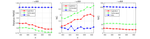
Figure 4: The relative RMSE, NC and NIC of three solvers under different $n$

Figure 4 plots the average relative RMSE, NC and NIC curves of three solvers under different sample sizes for Example 3. We see that three solvers have much higher relative RMSE than they do for Example 2, and NCL even fails in giving the desired estimator. The relative RMSE of CaZnRLS is a little (about $4\%$) higher than that of CoCoLasso. After checking the unbiased estimation $\Sigma$ of the covariance matrix of the true covariates, we find that the irrepresentable and minimum eigenvalue conditions in Datta and Zou (2017) are not satisfied. Now it is not clear whether our REC on $\mathcal{C}(\beta^{*})$ holds or not. This does not contradict to the theoretical analysis in Section 4 since now it is only known that our REC on $\mathcal{C}(\beta^{*})$ holds w.h.p. when $X$ is from Gaussian ensemble. The first subfigure indicates that it is very likely for our REC not to hold when $X$ is from the uniform distribution.

Case 2. Multiplicative errors

Example 4.

We generate $Z=X\circ M$ where the rows of $X$ are i.i.d. $\mathcal{N}(0,I)$, and the entries of $M$ are i.i.d. and follow the log-normal distribution, i.e., $\ln(M_{ij})$ are i.i.d and follow $N(0,\tau^{2}I)$ with $\tau=0.5$ or $0.8$.

Example 5.

We generate $Z$ in the same way as in Example 4 except that the entries of $X$ are i.i.d. and follow the Laplace distribution of mean 0 and variance 1.

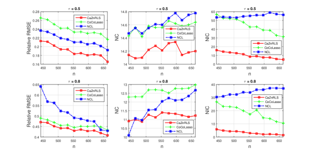
Figure 5: The relative RMSE, NC and NIC of three solvers under different $n$

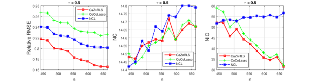
Figure 6: The relative RMSE, NC and NIC of three solvers under different $n$

Figure 5 and 6 plot the average relative RMSE, NC and NIC curves of three solvers under different $n$ for Example 4 and 5, respectively. By comparing Figure 5 with Figure 3, we see that CaZnRLS and CoCoLasso have the similar performance as they do for the additive errors. That is, CaZnRLS is better than CoCoLasso in terms of the relative RMSE and NIC whether for $X$ corrupted by high noise or low noise, though its NC is (at most $2$) fewer than the NC of CoCoLasso. Along with Figure 6, we conclude that CaZnRLS has the similar performance when the rows of $X$ follow the Gaussian and Laplace distribution.

Case 3. Missing data case

Example 6.

We generate $(Z_{ij})_{n\times p}$ for $Z_{ij}=X_{ij}$ with probability $1-\tau$ and $Z_{ij}=0$ with probability $\tau$ for $\tau=0.3$ or $0.5$, where the rows of $X$ are i.i.d. and obey the standard normal distribution $\mathcal{N}(0,I)$.

Example 7.

We generate $Z$ in the same way as in Example 6 except that $X_{ij}$ are i.i.d. and obey the exponential with mean 1 and variance 1.

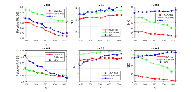
Figure 7: The relative RMSE, NC and NIC of three solvers under different $n$

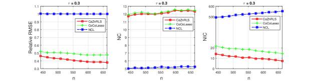
Figure 8: The relative RMSE, NC and NIC of three solvers under different $n$

Figure 7 and 8 plot the average relative RMSE, NC and NIC curves of three solvers under different $n$ for Example 6 and 7, respectively. Comparing Figure 7 with Figure 3 or 5, we see that the three solvers have similar performance as they do for the additive and multiplicative errors. In fact, we check that similar to Example 2 and 4-5, Example 6 satisfies the irrepresentable and minimum eigenvalue conditions in Datta and Zou (2017) when $n\geq\lfloor 4.4s\ln(p)\rfloor$. Of course, our REC on $\mathcal{C}(\beta^{*})$ holds with a high probability for Example 2 and 4, and Figure 6-8 also indicate that our REC holds with a high probability when the rows of $X$ follow the Laplace and exponential distributions. Figure 8 shows that, when the entries of $X$ follow the exponential distribution, CaZnRLS is superior to the other two solvers in terms of the relative RMSE and NIC, and its RMSE improves that of CoCoLasso at least $11\%$. Now NCL fails in yielding the desired estimator. After checking, we find that Example 7 actually does not satisfy the irrepresentable and minimum eigenvalue conditions in Datta and Zou (2017). Now it is not clear whether our REC holds or not for this example.

Motivated by one referee’s comments, we next provide an example that does not satisfy the irrepresentable condition but our REC holds w.h.p..

Example 8.

We generate $Z=X+A$ with $p=250$ where the entries of $X_{S^{*}}$ are i.i.d. $\mathcal{N}(0,1)$, the entries of $X_{(S^{*})^{c}}$ are i.i.d. $\mathcal{N}(0,5^{2})$, and the rows of $A$ are generated in the same way as in Example 2 with $\tau=0.75$.

Figure 9 plots the average relative RMSE, NC and NIC curves of CaZnRLS and CoCoLasso under different $n$ for Example 8. Since NCL fails in this example, we do not include its results in Figure 9. We see that the relative RMSE of CaZnRLS is lower than that of CoCoLasso, and when $n\geq\lfloor 5s\ln(p)\rfloor$, the relative RMSE of CaZnRLS improves at least $10\%$ that of CoCoLasso. The NC and NIC of CoCoLasso are still higher than those of CaZnRLS, but NC of the latter is at most $1$ lower than that of the former. This example further confirms the theoretical results in Section 4.

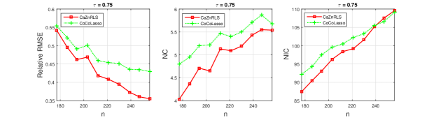
Figure 9: The relative RMSE, NC and NIC of three solvers under different $n$

5.2. Fixed locations of the nonzero entries of $\beta^{*}$

As one referee pointed out, it would be interesting to show the effects of the correlation between the predictors on the performance of three solvers. In this part, we test whether the correlation between the predictors has an effect on the performance of three solvers or not, by using the examples generated by Datta and Zou (2017) in which the locations of the nonzero entries of $\beta^{*}$ are fixed. Specifically, $\beta^{*}=(3,1.5,0,0,2,0,\ldots,0)$ with the number of nonzero entries $s=3$. The data $X$ is generated with $p=250$ and $n=100$ such that the rows of $X$ obey i.i.d. $\mathcal{N}(0,\Sigma_{X})$ for $(\Sigma_{X})_{ij}=0.5^{|i-j|}$. Table 1 summaries the simulation results of three solvers for additive errors, multiplicative errors and missing data, where the error matrices $A$ and $M$ for the additive and multiplicative errors are generated in the same way as in Example 2 and 4 respectively, while the contaminated matrix $Z$ in missing data is generated in the same way as in Example 6.

Table 1: The average relative RMSE, NC and NIC of three solvers

	Additive errors			Multiplicative errors			Missing data
	$\tau=1$			$\tau=0.8$			$\tau=0.5$
	​CaZnRLS​	​CoCoLasso​	​NCL​	​CaZnRLS​	​CoCoLasso​	​NCL​	​CaZnRLS​	​CoCoLasso	​NCL
RMSE	0.410	0.492	0.535	0.370	0.524	0.600	0.447	0.521	0.528
NC	2.81	2.87	2.41	2.76	2.87	2.18	2.69	2.75	2.27
NIC	1.48	2.46	6.48	1.30	2.48	5.31	2.41	2.60	6.90

From Table 1, CaZnRLS yields the lowest relative RMSE and NIC for three classes of measurement errors though its NC is a little fewer than that of CoCoLasso, while NCL yields the highest relative RMSE and NIC. By comparing with the numerical comparison results in Section 5.1, the three solvers have similar performance as they do for those examples where the locations of the nonzero entries of $\beta^{*}$ are not fixed. That is, the correlation between the predictors has little influence on their performance.

From the numerical comparisons in the last two subsections, when the true covariate matrix $X$ comes from the standard normal distribution (now our REC holds with a high probability) or other distributions such as the Laplace one in Example 5 and the exponential one in Example 7, CaZnRLS is superior to CoCoLasso in terms of relative RMSE (especially for low noise cases) and NIC, although its NC is a little lower than that of CoCoLasso. As shown in Figure 10, CaZnRLS requires much less computing time.

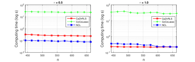
Figure 10: The computing time of three solvers for Example 2

Supplementary Materials

Appendix A

In this part, we write $\Delta\beta^{k}=\beta^{k}-\beta^{*}$ and $v^{k}=e-w^{k}$ for $k=1,2,\ldots$.

A.1. The proof of Theorem 2

To get the conclusion of Theorem 2, we need the following two lemmas.

Lemma 1.

For any $\beta\in\mathbb{R}^{p}$, it holds that $\frac{1}{2n}\|\widetilde{Z}\beta\|^{2}\geq\frac{1}{2n}\|X\beta\|^{2}+\frac{1}{2}\beta^{\mathbb{T}}D\beta$.

Proof.

From $\widetilde{\Sigma}=\frac{1}{n}\widetilde{Z}^{\mathbb{T}}\widetilde{Z}$ and $\widetilde{\Sigma}=\widehat{\epsilon}I+\Pi_{\mathbb{S}_{+}^{p}}(\widehat{\Sigma}-\widehat{\epsilon}I)$, for any $\beta\in\mathbb{R}^{p}$, we get

$$\frac{1}{2n}\big{\|}\widetilde{Z}\beta\big{\|}^{2} =\frac{1}{2n}\|X\beta\|^{2}+\frac{1}{2}\beta^{\mathbb{T}}(\widetilde{\Sigma}-\widehat{\Sigma})\beta+\frac{1}{2}\beta^{\mathbb{T}}(\widehat{\Sigma}-\Sigma)\beta$$

$$=\frac{1}{2n}\|X\beta\|^{2}+\frac{1}{2}\beta^{\mathbb{T}}\Pi_{\mathbb{S}_{+}^{p}}(\widehat{\epsilon}I-\widehat{\Sigma})\beta+\frac{1}{2}\beta^{\mathbb{T}}D\beta$$

$$\geq\frac{1}{2n}\|X\beta\|^{2}+\frac{1}{2}\beta^{\mathbb{T}}D\beta$$

where the inequality is by the positive semidefiniteness of $\Pi_{\mathbb{S}_{+}^{p}}(\widehat{\epsilon}I-\widehat{\Sigma})$. ∎

Lemma 2.

Suppose that for some $k\geq 1$ there exists an index set $S^{k-1}\supseteq S^{*}$ such that $\max_{i\in(S^{k-1})^{c}}w^{k-1}_{i}\!\leq\frac{1}{2}.$ Then, whenever $\lambda\geq 8\|\widetilde{\varepsilon}\|_{\infty}$, it holds that

$$\|\Delta\beta^{k}_{(S^{k-1})^{c}}\|_{1}\leq 3\|\Delta\beta^{k}_{S^{k-1}}\|_{1},\qquad\qquad\qquad$$

$$\frac{1}{2n}\big{\|}\widetilde{Z}\Delta\beta^{k}\big{\|}^{2}\leq\Big{(}\|\widetilde{\varepsilon}_{\!S^{k-1}}\|+\lambda\sqrt{{\textstyle\sum_{i\in S^{*}}}(v^{k-1}_{i})^{2}}\Big{)}\big{\|}\Delta\beta_{\!S^{k-1}}^{k}\big{\|}.$$

Proof.

From the optimality of $\beta^{k}$ and the feasibility of $\beta^{*}$ to (3.1), we have

$$\frac{1}{2n}\big{\|}\widetilde{Z}\beta^{k}-\widetilde{y}\big{\|}^{2}+\lambda\sum_{i=1}^{p}v_{i}^{k-1}\big{|}\beta^{k}_{i}\big{|}\leq\frac{1}{2n}\big{\|}\widetilde{Z}\beta^{*}-\widetilde{y}\big{\|}^{2}+\lambda\sum_{i=1}^{p}v_{i}^{k-1}\big{|}\beta^{*}_{i}\big{|}$$

which, by $\Delta\beta^{k}\!=\beta^{k}-\beta^{*}$ and $\widetilde{\varepsilon}\!=\frac{1}{n}\widetilde{Z}^{\mathbb{T}}(\widetilde{y}-\widetilde{Z}\beta^{*})$, can be rearranged as

$$\frac{1}{2n}\big{\|}\widetilde{Z}\Delta\beta^{k}\big{\|}^{2} \leq\langle\widetilde{\varepsilon},\Delta\beta^{k}\rangle+\lambda\!\sum_{i\in S^{*}}v_{i}^{k-1}\left(\big{|}\beta^{*}_{i}\big{|}-\big{|}\beta^{k}_{i}\big{|}\right)-\lambda\!\sum_{i\in(S^{*})^{c}}v_{i}^{k-1}\big{|}\beta^{k}_{i}\big{|}$$

$$\leq\langle\widetilde{\varepsilon},\Delta\beta^{k}\rangle+\lambda\!\sum_{i\in S^{*}}v^{k-1}_{i}\big{|}\Delta\beta^{k}_{i}\big{|}-\lambda\!\sum_{i\in(S^{k-1})^{c}}\!v^{k-1}_{i}\big{|}\Delta\beta^{k}_{i}\big{|}$$ (5.9)

$$\leq\sum_{i\in S^{k-1}}\big{|}\widetilde{\varepsilon}_{i}\big{|}\big{|}\Delta\beta^{k}_{i}\big{|}+\sum_{i\in(S^{k-1})^{c}}\big{|}\widetilde{\varepsilon}_{i}\big{|}\big{|}\Delta\beta^{k}_{i}\big{|}$$

$$\quad\ +\lambda\!\sum_{i\in S^{*}}v^{k-1}_{i}\big{|}\Delta\beta^{k}_{i}\big{|}-\lambda\!\sum_{i\in(S^{k-1})^{c}}\!v^{k-1}_{i}\big{|}\Delta\beta^{k}_{i}\big{|}$$

$$\leq(\lambda+\!\|\widetilde{\varepsilon}\|_{\infty})\big{\|}\Delta\beta^{k}_{S^{k-1}}\big{\|}_{1}+\big{(}\|\widetilde{\varepsilon}\|_{\infty}\!-\!\lambda/2\big{)}\big{\|}\Delta\beta^{k}_{(S^{k-1})^{c}}\big{\|}_{1}$$

where the second inequality is using $S^{k-1}\supseteq S^{*}$, and the last one is due to $v_{i}^{k}\leq 1$ for $i\in S^{*}$ and $\min_{i\notin S^{k-1}}v^{k-1}_{i}\geq\frac{1}{2}$. From $\lambda\geq 8\|\widetilde{\varepsilon}\|_{\infty}$ and $\frac{1}{2n}\big{\|}\widetilde{Z}\Delta\beta^{k}\big{\|}^{2}\geq 0$, we obtain the first inequality. For the second inequality, by using inequality (5) and $\min_{i\notin S^{k-1}}v^{k-1}_{i}\geq\frac{1}{2}$, it follows that

$$\frac{1}{2n}\big{\|}\widetilde{Z}\Delta\beta^{k}\big{\|}^{2} \leq\sum_{i=1}^{p}|\widetilde{\varepsilon}_{i}||\Delta\beta^{k}_{i}|-\frac{1}{2}\lambda\!\sum_{i\in(S^{k-1})^{c}}\!\big{|}\Delta\beta^{k}_{i}\big{|}+\lambda\!\sum_{i\in S^{*}}v^{k-1}_{i}\big{|}\Delta\beta^{k}_{i}\big{|}$$

$$\leq\sum_{i\in S^{k-1}}\big{|}\widetilde{\varepsilon}_{i}\big{|}\big{|}\Delta\beta^{k}_{i}\big{|}+\lambda\textstyle\sum_{i\in S^{*}}v^{k-1}_{i}\big{|}\Delta\beta^{k}_{i}\big{|}$$

$$\leq\|\widetilde{\varepsilon}_{\!S^{k-1}}\|\big{\|}\Delta\beta_{\!S^{k-1}}^{k}\big{\|}+\lambda\!\sqrt{{\textstyle\sum_{i\in S^{*}}}(v^{k-1}_{i})^{2}}\,\big{\|}\Delta\beta_{\!S^{k-1}}^{k}\big{\|},$$

where the second inequality is due to $\lambda\geq 8\|\widetilde{\varepsilon}\|_{\infty}$. ∎

The proof of Theorem 2: Define $S^{k-1}\!:=S^{*}\cup\{i\notin S^{*}\!:w_{i}^{k-1}>\frac{1}{2}\}$ for each $k\in\mathbb{N}$. We first argue that if $|S^{l-1}|\leq 1.5s$ for some $l\in\mathbb{N}$, and consequently the following inequality holds

$$\big{\|}\Delta\beta^{l}\big{\|}\leq\frac{2(\|\widetilde{\varepsilon}\|_{\infty}\sqrt{1.5s}+\lambda\sqrt{s})}{\kappa-24s\|D\|_{\rm max}}\leq\frac{(2+\!\sqrt{6}/8)\lambda\!\sqrt{s}}{\kappa-24s\|D\|_{\rm max}}.$$ (5.10)

Since $S^{l-1}\supseteq S^{*}$ with $|S^{l-1}|\leq 1.5s$ and $\lambda\geq 8\|\widetilde{\varepsilon}\|_{\infty}$, from Lemma 2 we have

$$\frac{1}{2n}\big{\|}\widetilde{Z}\Delta\beta^{l}\big{\|}^{2} \leq\left[\|\widetilde{\varepsilon}_{\!S^{l-1}}\|+\lambda\!\sqrt{{\textstyle\sum_{i\in S^{*}}}(v^{l-1}_{i})^{2}}\right]\big{\|}\Delta\beta_{\!S^{l-1}}^{l}\big{\|},$$

$$\big{|}(\Delta\beta^{l})^{\mathbb{T}}D\Delta\beta^{l}\big{|} \leq\|D\|_{\rm max}\|\Delta\beta^{l}\|_{1}^{2}=\|D\|_{\rm max}\big{(}\|\Delta\beta^{l}_{S^{l-1}}\|_{1}+\|\Delta\beta^{l}_{(S^{l-1})^{c}}\|_{1}\big{)}^{2}$$

$$\leq 16\|D\|_{\rm max}\|\Delta\beta^{l}_{S^{l-1}}\|_{1}^{2}\leq 16|S^{l-1}|\|D\|_{\rm max}\|\Delta\beta^{l}_{S^{l-1}}\|^{2}$$

$$\leq 24s\|D\|_{\rm max}\|\Delta\beta_{S^{l-1}}^{l}\|^{2}.$$ (5.11)

By combining the last two inequalities with Lemma 1, it then follows that

$$\frac{1}{2n}\big{\|}X\Delta\beta^{l}\big{\|}^{2}-12s\|D\|_{\rm max}\|\Delta\beta^{l}\|^{2}\leq\left[\|\widetilde{\varepsilon}_{\!S^{l-1}}\|+\lambda\!\sqrt{{\textstyle\sum_{i\in S^{*}}}(v^{l-1}_{i})^{2}}\right]\big{\|}\Delta\beta_{\!S^{l-1}}^{l}\big{\|}.$$

Notice that $\Delta\beta^{l}\in\mathcal{C}(S^{*})$ since $S^{l-1}\supseteq S^{*}$ with $|S^{l-1}|\leq 1.5s$. Together with the $\kappa$-REC of $\Sigma$ on $\mathcal{C}(S^{*})$, it is immediate to obtain

$$\!\frac{1}{2}\big{(}\kappa-24s\|D\|_{\rm max}\big{)}\|\Delta\beta^{l}\|^{2} \leq\left[\|\widetilde{\varepsilon}_{\!S^{l-1}}\|+\lambda\!\sqrt{{\textstyle\sum_{i\in S^{*}}}(v^{l-1}_{i})^{2}}\right]\big{\|}\Delta\beta_{\!S^{l-1}}^{l}\big{\|}$$ (5.12)

$$\leq\big{[}\|\widetilde{\varepsilon}\|_{\infty}\sqrt{|S^{l-1}|}+\lambda\sqrt{s}\big{]}\big{\|}\Delta\beta^{l}\big{\|}$$

$$\leq\big{[}\|\widetilde{\varepsilon}\|_{\infty}\sqrt{1.5s}+\lambda\sqrt{s}\big{]}\big{\|}\Delta\beta^{l}\big{\|}.$$

This, by $\|\widetilde{\varepsilon}\|_{\infty}\leq\frac{1}{8}\lambda$, implies that the inequality (5.10) holds.

Next we show that $|S^{k-1}|\!\leq 1.5s$ for all $k\in\mathbb{N}$. When $k=1$, this inequality holds automatically since $S^{0}=S^{*}$ implied by $w^{0}\leq\frac{1}{2}e$. Now assume that $|S^{k-1}|\leq 1.5s$ for $k=l$ with $l\geq 1$. From the above argument, we have $\|\beta^{l}\!-\beta^{*}\|\leq\frac{(2+\!\sqrt{6}/8)\lambda\!\sqrt{s}}{\kappa-24s\|D\|_{\rm max}}.$ Notice that $i\in S^{l}\backslash S^{*}$ implies $i\notin S^{*}$ and $w_{i}^{l}\in(\frac{1}{2},1]$. By equation (3.3), the latter implies $\rho_{l}|\beta^{l}_{i}|\geq 1$. Consequently,

$$\sqrt{|S^{l}\backslash S^{*}|} \leq\sqrt{{\textstyle\sum_{i\in S^{l}\backslash S^{*}}}(\rho_{l}|\beta^{l}_{i}|)^{2}}\leq\rho_{l}\|\beta^{l}-\beta^{*}\|$$

$$\leq\frac{(2+\!\sqrt{6}/8)\rho_{l}\lambda\!\sqrt{s}}{\kappa-24s\|D\|_{\rm max}}\leq\sqrt{0.5s}$$ (5.13)

where the last inequality is by $\rho_{l}\lambda\leq\rho_{3}\lambda\leq\frac{2(\kappa-24s\|D\|_{\rm max})}{5\sqrt{2}}$. Thus, $|S^{l}|\leq 1.5s$. Hence, $|S^{k-1}|\leq 1.5s$ for all $k\in\mathbb{N}$, and the error bound follows from (5.10).

A.2. The proof of Theorem 3

To achieve the conclusion of Theorem 3, we need the following lemma.

Lemma 3.

Let $F^{k}$ and $\Lambda^{k}$ be the sets in (4.6). Then, for each $k\in\{0\}\cup\mathbb{N}$,

$$\sqrt{{\textstyle\sum_{i\in S^{*}}}(v^{k}_{i})^{2}}\leq\sqrt{{\textstyle\sum_{i\in S^{*}}}\max(\mathbb{I}_{\Lambda^{k}}(i),\mathbb{I}_{F^{k}}(i))}.$$

Proof.

Fix an arbitrary $i\in S^{*}$. If $i\in F^{k}$, from $v^{k}_{i}=1-w_{i}^{k}\leq 1$ we have $v^{k}_{i}\leq\mathbb{I}_{F^{k}}(i)$. If $i\notin F^{k}$, from $v^{k}_{i}=1-w_{i}^{k}$ and (3.3), it follows that $v_{i}^{k}=\max\big{(}0,\min(1,\frac{2a-(a+1)\rho_{k}|\beta_{i}^{k}|}{2(a-1)})\big{)},$ and hence $v_{i}^{k}\leq\mathbb{I}_{\{i:\,\rho_{k}|\beta^{k}_{i}|\leq 2a/(a+1)\}}(i)\leq\mathbb{I}_{\Lambda^{k}}(i).$ Thus, for each $i$, it holds that $(v^{k}_{i})^{2}\leq v^{k}_{i}\leq\max(\mathbb{I}_{\Lambda^{k}}(i),\mathbb{I}_{F^{k}}(i)).$ From this, it is immediate to obtain the desired result. ∎

The proof of Theorem 3: Write $S^{k-1}:=S^{*}\cup\{i\notin S^{*}\!:w_{i}^{k-1}>\frac{1}{2}\}$ for each $k\in\mathbb{N}$. Since the conclusion holds automatically for $k=1$, it suffices to consider the case $k\geq 2$. From the proof of Theorem 2, we know that $|S^{k-1}|\leq 1.5s$ for all $k\in\mathbb{N}$. Moreover, by using (5) and $\rho_{k}\geq 1$,

$$\big{\|}\widetilde{\varepsilon}_{\!S^{k-1}}\big{\|}\leq\big{\|}\widetilde{\varepsilon}_{\!S^{*}}\big{\|}+\sqrt{|S^{k-1}\backslash S^{*}|}\big{\|}\widetilde{\varepsilon}\big{\|}_{\infty}\leq\big{\|}\widetilde{\varepsilon}_{\!S^{*}}\big{\|}+\frac{\rho_{k-1}\lambda}{8}\sqrt{|S^{k-1}\backslash S^{*}|}.$$ (5.14)

By using inequality (5.12) and Lemma 3, it follows that

$$\|\beta^{k}-\beta^{*}\|\leq\frac{2}{\kappa-24s\|D\|_{\rm max}}\left[\|\widetilde{\varepsilon}_{\!S^{k-1}}\|+\lambda\!\sqrt{{\textstyle\sum_{i\in S^{*}}}(v^{k-1}_{i})^{2}}\right]$$

$$\leq\frac{2}{\kappa-\!24s\|D\|_{\rm max}}\left[\|\widetilde{\varepsilon}_{\!S^{k-1}}\|+\lambda\!\sqrt{{\textstyle\sum_{i\in S^{*}}}\max(\mathbb{I}_{\Lambda^{k-1}}(i),\mathbb{I}_{F^{k-1}}(i))}\right]$$

$$\leq\frac{2}{\kappa-\!24s\|D\|_{\rm max}}\left[\|\widetilde{\varepsilon}_{\!S^{k-1}}\|+\lambda\!\sqrt{{\textstyle\sum_{i\in S^{*}}}\max\big{(}\mathbb{I}_{\Lambda^{k-1}}(i),\big{|}|\beta^{k-1}_{\!{}_{i}}|-|\beta^{*}_{i}|\big{|}^{2}(\rho_{k-1})^{2}\big{)}}\right]$$

$$\leq\frac{2}{\kappa-\!24s\|D\|_{\rm max}}\Big{(}\|\widetilde{\varepsilon}_{\!S^{k-1}}\|+\lambda\sqrt{\max\big{(}{\textstyle\sum_{i\in S^{*}}}\mathbb{I}_{\Lambda^{k-1}}(i),(\rho_{k-1})^{2}\|\Delta\beta^{k-1}\|^{2}\big{)}}\Big{)}$$

where the third inequality is by the definition of $F^{k-1}$. Together with (5.14),

$$\|\beta^{k}-\beta^{*}\| \leq\frac{2}{\kappa-\!24s\|D\|_{\rm max}}\Big{[}\big{\|}\widetilde{\varepsilon}_{\!S^{*}}\big{\|}+\lambda\!\sqrt{{\textstyle\sum_{i\in S^{*}}}\mathbb{I}_{\Lambda^{k-1}}(i)}+\frac{9\rho_{k-1}\lambda}{8}\big{\|}\Delta\beta^{k-1}\big{\|}\Big{]}$$

$$\leq\frac{2}{\kappa-\!24s\|D\|_{\rm max}}\Big{(}\big{\|}\widetilde{\varepsilon}_{\!S^{*}}\big{\|}+\lambda\!\sqrt{{\textstyle\sum_{i\in S^{*}}}\,\mathbb{I}_{\Lambda^{k-1}}(i)}\Big{)}+\frac{1}{\sqrt{2}}\|\beta^{k-1}-\beta^{*}\|$$

where the second inequality is using $\rho_{k-1}\lambda\leq\rho_{3}\lambda\leq\frac{2(\kappa-24s\|D\|_{\rm max})}{5\sqrt{2}}$. The desired result follows by solving this recursion with respect to $\|\beta^{k}-\beta^{*}\|$.

A.3. The proof of Theorem 4

We need the following two lemmas with $\Delta\widehat{\beta}^{k}=\beta^{k}-\beta^{\rm LS}$ for $k=1,2,\ldots$.

Lemma 4.

Suppose that for some $k\geq 1$ there exists an index set $S^{k-1}\supseteq S^{*}$ such that $\max_{i\in(S^{k-1})^{c}}w^{k-1}_{i}\!\leq\frac{1}{2}$. Then, whenever $\lambda\geq 6\|\varepsilon^{{\rm LS}}\|_{\infty}$, it holds that

$$\|\Delta\widehat{\beta}^{k}_{(S^{k-1})^{c}}\|_{1}\leq 3\|\Delta\widehat{\beta}^{k}_{S^{k-1}}\|_{1}.$$

Proof.

By the optimality of $\beta^{k}$ and the feasibility of $\beta^{{\rm LS}}$ to (3.1), we have

$$\frac{1}{2n}\big{\|}\widetilde{Z}\beta^{k}-\widetilde{y}\big{\|}^{2}+\lambda\sum_{i=1}^{p}v_{i}^{k-1}\big{|}\beta^{k}_{i}\big{|}\leq\frac{1}{2n}\big{\|}\widetilde{Z}\beta^{{\rm LS}}-\widetilde{y}\big{\|}^{2}+\lambda\sum_{i=1}^{p}v_{i}^{k-1}\big{|}\beta^{{\rm LS}}_{i}\big{|},$$

which, by $\Delta\widehat{\beta}^{k}=\beta^{k}-\beta^{\rm LS}$ and $\varepsilon^{{\rm LS}}=\frac{1}{n}\widetilde{Z}^{\mathbb{T}}(\widetilde{y}-\widetilde{Z}\beta^{\rm LS})$, can be rearranged as

$$\frac{1}{2n}\big{\|}\widetilde{Z}\Delta\widehat{\beta}^{k}\big{\|}^{2} \leq\langle\varepsilon^{{\rm LS}},\Delta\widehat{\beta}^{k}\rangle+\lambda\sum_{i=1}^{p}v_{i}^{k-1}(|\beta^{{\rm LS}}_{i}|-|\beta^{k}_{i}|)$$

$$=\sum_{i\notin S^{*}}\varepsilon_{i}^{{\rm LS}}\Delta\widehat{\beta}_{i}^{k}+\lambda\sum_{i\in S^{*}}v_{i}^{k-1}(\big{|}\beta^{{\rm LS}}_{i}\big{|}-\big{|}\beta^{k}_{i}\big{|})-\lambda\sum_{i\notin S^{*}}v_{i}^{k-1}\big{|}\beta^{k}_{i}\big{|}$$

$$\leq\sum_{i\notin S^{*}}\big{|}\varepsilon^{{\rm LS}}_{i}\big{|}\big{|}\Delta\widehat{\beta}^{k}_{i}\big{|}+\lambda\sum_{i\in S^{*}}v^{k-1}_{i}\big{|}\Delta\widehat{\beta}^{k}_{i}\big{|}-\lambda\sum_{i\notin S^{*}}v^{k-1}_{i}\big{|}\beta^{k}_{i}\big{|}$$

where the equality is using $\varepsilon^{{\rm LS}}_{i}=0$ for $i\in S^{*}$ and $\beta^{{\rm LS}}_{i}=0$ for all $i\notin S^{*}$. Now from $S^{k-1}\supseteq S^{*}$ and $v_{i}^{k-1}=1-w_{i}^{k-1}\geq 1/2$ for $i\notin S^{k-1}$, we obtain

$$\frac{1}{2n}\big{\|}\widetilde{Z}\Delta\widehat{\beta}^{k}\big{\|}^{2} \leq\sum_{i\notin S^{*}}\big{|}\varepsilon^{{\rm LS}}_{i}\big{|}\big{|}\Delta\widehat{\beta}_{i}^{k}\big{|}+\lambda\!\sum_{i\in S^{*}}v^{k-1}_{i}|\Delta\widehat{\beta}^{k}_{i}|-\lambda\!\sum_{i\notin S^{k-1}}v^{k-1}_{i}\big{|}\Delta\widehat{\beta}^{k}_{i}\big{|}$$

$$\leq\sum_{i\in S^{k-1}\backslash S^{*}}\big{|}\varepsilon^{{\rm LS}}_{i}\big{|}\big{|}\Delta\widehat{\beta}^{k}_{i}\big{|}+\lambda\!\sum_{i\in S^{*}}v^{k-1}_{i}\big{|}\Delta\widehat{\beta}^{k}_{i}\big{|}$$

$$\qquad+\sum_{i\in(S^{k-1})^{c}}\big{|}\varepsilon^{{\rm LS}}_{i}\big{|}\big{|}\Delta\widehat{\beta}^{k}_{i}\big{|}-\frac{1}{2}\lambda\big{\|}\Delta\widehat{\beta}^{k}_{(S^{k-1)^{c}}}\big{\|}_{1}$$ (5.15)

$$\leq\max\big{(}\|\varepsilon^{{\rm LS}}\|_{\infty},\lambda\big{)}\big{\|}\Delta\widehat{\beta}_{S^{k-1}}^{k}\big{\|}_{1}+\!\big{(}\|\varepsilon^{{\rm LS}}\|_{\infty}\!-\frac{1}{2}\lambda\big{)}\big{\|}\Delta\widehat{\beta}^{k}_{(S^{k-1})^{c}}\big{\|}_{1}$$

which along with the nonnegativity of $\frac{1}{2n}\|\widetilde{Z}\Delta\widehat{\beta}^{k}\|^{2}$ implies the result. ∎

Lemma 5.

Suppose that for some $k\geq 1$ there exists $S^{k-1}\supseteq S^{*}$ with $|S^{k-1}|\leq 1.5s$ such that $\max_{i\in(S^{k-1})^{c}}w^{k-1}_{i}\!\leq\frac{1}{2}$, and that the matrix $\Sigma$ satisfies the $\kappa$-REC on $\mathcal{C}(S^{*})$ with $\kappa>24s\|D\|_{\rm max}$. Then, when $\lambda\geq 6\|\varepsilon^{{\rm LS}}\|_{\infty}$,

$$\big{\|}\Delta\widehat{\beta}^{k}\big{\|}\leq\frac{2}{\kappa-24s\|D\|_{\rm max}}\Big{(}\big{\|}\varepsilon^{\rm{LS}}_{\!S^{k-1}}\big{\|}+\lambda\sqrt{{\textstyle\sum_{i\in S^{*}}}(v^{k-1}_{i})^{2}}\Big{)}.$$

Proof.

First of all, from equation (5) and $\lambda\geq 6\|\varepsilon^{{\rm LS}}\|_{\infty}$, it follows that

$$\frac{1}{2n}\big{\|}\widetilde{Z}\Delta\widehat{\beta}^{k}\big{\|}^{2} \leq\sum_{i\in S^{k-1}\backslash S^{*}}\big{|}\varepsilon^{{\rm LS}}_{i}\big{|}\big{|}\Delta\widehat{\beta}^{k}_{i}\big{|}+\lambda\sum_{i\in S^{*}}v^{k-1}_{i}\big{|}\Delta\widehat{\beta}^{k}_{i}\big{|}$$

$$\leq\|\varepsilon_{S^{k-1}}^{{\rm LS}}\|\|\Delta\widehat{\beta}_{\!S^{k-1}}^{k}\|+\lambda\sqrt{{\textstyle\sum_{i\in S^{*}}}(v^{k-1}_{i})^{2}}\,\|\Delta\widehat{\beta}_{S^{k-1}}^{k}\|$$

where the second inequality is using $S^{k-1}\supseteq S^{*}$. Together with Lemma 1,

$$\frac{1}{2n}\big{\|}X\Delta\widehat{\beta}^{k}\big{\|}^{2}\leq\Big{[}\|\varepsilon_{S^{k-1}}^{{\rm LS}}\|+\lambda\sqrt{{\textstyle\sum_{i\in S^{*}}}(v^{k-1}_{i})^{2}}\Big{]}\big{\|}\Delta\widehat{\beta}_{\!S^{k-1}}^{k}\big{\|}-\frac{1}{2}(\Delta\widehat{\beta}^{k})^{\mathbb{T}}D\Delta\widehat{\beta}^{k}.$$

Since $S^{k-1}\!\supseteq S^{*}$ with $|S^{k-1}|\!\leq 1.5s$, using Lemma 4 and the same arguments as for (5) yields that $-(\Delta\widehat{\beta}^{k})^{\mathbb{T}}D\Delta\widehat{\beta}^{k}\leq 24s\|D\|_{\rm max}\|\Delta\widehat{\beta}^{k}\|^{2}$. Then,

$$\frac{1}{2n}\big{\|}X\Delta\widehat{\beta}^{k}\big{\|}^{2}-12s\|D\|_{\rm max}\|\Delta\widehat{\beta}^{k}\|^{2}\leq\Big{[}\|\varepsilon_{S^{k-1}}^{{\rm LS}}\|+\lambda\sqrt{{\textstyle\sum_{i\in S^{*}}}(v^{k-1}_{i})^{2}}\Big{]}\big{\|}\Delta\widehat{\beta}_{\!S^{k-1}}^{k}\big{\|}.$$

Since $\Sigma$ satisfies the $\kappa$-RSC on the set $\mathcal{C}(S^{*})$ with $\kappa>24s\|D\|_{\rm max}$, we have

$$\frac{1}{2}(\kappa-24s\|D\|_{\rm max})\big{\|}\Delta\widehat{\beta}^{k}\big{\|}^{2}\leq\Big{[}\|\varepsilon_{S^{k-1}}^{{\rm LS}}\|+\lambda\sqrt{{\textstyle\sum_{i\in S^{*}}}(v^{k-1}_{i})^{2}}\Big{]}\big{\|}\Delta\widehat{\beta}_{\!S^{k-1}}^{k}\big{\|}.$$

This implies the desired result. The proof is then completed. ∎

The proof of Theorem 4: Let $S^{k-1}:=S^{*}\cup\{i\notin S^{*}\!:w_{i}^{k-1}>\frac{1}{2}\}$ for each $k\in\mathbb{N}$. We first prove that the desired inequalities holds by the induction on $k\in\mathbb{N}$. Since $w^{0}\leq\frac{1}{2}e$, we have $S^{0}=S^{*}$ and $|S^{0}|=s$. Notice that $\Sigma$ satisfies the $\kappa$-REC on $\mathcal{C}(S^{*})$ with $\kappa>24s\|D\|_{\rm max}$ and $\lambda\geq 6\|\varepsilon^{\rm{LS}}\|_{\infty}$. The conditions of Lemma 5 are satisfied. Along with $\varepsilon^{\rm{LS}}_{\!S^{*}}=0$ and $F^{0}=S^{*}$,

$$\|\beta^{1}-\beta^{\rm{LS}}\| \leq\frac{2}{\gamma}\Big{(}\|\varepsilon^{\rm{LS}}_{\!S^{0}}\|+\!\lambda\sqrt{{\textstyle\sum_{i\in S^{*}}}(v^{0}_{i})^{2}}\Big{)}$$

$$\leq\frac{2}{\gamma}\Big{(}\|\varepsilon^{\rm{LS}}_{\!S^{*}}\|+\!\lambda\sqrt{|F^{0}|}\Big{)}\leq\frac{2.03\rho_{0}\lambda\sqrt{|F^{0}|}}{\gamma}.$$ (5.16)

Since $|\beta^{\rm{LS}}_{i}-\beta^{*}_{i}|\leq\|\widetilde{\varepsilon}^{\dagger}\|_{\infty}$ for $i\in S^{*}$ by (4.8) and $\rho_{1}\geq\gamma\lambda^{-1}\|\widetilde{\varepsilon}^{\dagger}\|_{\infty}$, we have

$$|\beta^{\rm{LS}}_{i}\!-\beta^{1}_{i}|\geq|\beta^{*}_{i}\!-\beta^{1}_{i}|-|\beta^{*}_{i}\!-\beta^{\rm{LS}}_{i}|\geq\frac{1}{\rho_{1}}-\frac{\rho_{1}\lambda}{\gamma}\geq\frac{9\sqrt{3}-4}{9\sqrt{3}\rho_{1}}\quad\forall i\in F^{1}$$

where the last inequality is by $1\leq\rho_{1}\leq\sqrt{\frac{4\gamma}{9\sqrt{3}\lambda}}$. By the last two equations,

$$\sqrt{|F^{1}|}=\sqrt{{\textstyle\sum_{i=1}^{p}}\mathbb{I}_{F^{1}}(i)}\leq\frac{9\sqrt{3}\rho_{1}}{9\sqrt{3}\!-\!4}\sqrt{{\textstyle\sum_{i=1}^{p}}|\beta^{\rm{LS}}_{i}-\beta^{1}_{i}|^{2}}\leq\frac{18.27\sqrt{3}\rho_{1}\rho_{0}\lambda}{(9\sqrt{3}\!-\!4)\gamma}\sqrt{|F^{0}|}.$$

Together with (5) and $1=\rho_{0}<\rho_{1}\leq\rho_{3}$, we conclude that the desired inequalities holds for $k=1$. Now, assuming that the conclusion holds for $k\leq l-1$ with $l\geq 2$, we prove that the conclusion holds for $k=l$. For this purpose, we first argue $|S^{l-1}|\leq 1.5s$. Indeed, for $i\in S^{l-1}\backslash S^{*}$, we have $w_{i}^{l-1}\in(\frac{1}{2},1]$, which by (3.3) implies that $\rho_{l-1}|\beta^{l-1}_{i}|\geq 1$. Then,

$$\sqrt{|S^{l-1}\backslash S^{*}|} \leq\sqrt{|F^{l-1}|}\leq\frac{18.27\sqrt{3}\rho_{l-1}\rho_{l-2}\lambda}{(9\sqrt{3}\!-\!4)\gamma}\sqrt{|F^{l-2}|}\leq\cdots$$

$$\leq\Big{(}\frac{18.27\sqrt{3}\lambda}{(9\sqrt{3}\!-\!4)\gamma}\Big{)}^{l-1}\rho_{l-1}\rho_{l-2}^{2}\cdots\rho_{2}^{2}\rho_{1}\sqrt{|F^{0}|}$$

$$\leq\sqrt{\Big{(}\frac{18.27\sqrt{3}(\rho_{3})^{2}\lambda}{(9\sqrt{3}\!-\!4)\gamma}\Big{)}^{2l-2}|F^{0}|}\leq\sqrt{\Big{(}\frac{8.12}{9\sqrt{3}\!-\!4}\Big{)}^{2l-2}|F^{0}|}\leq\sqrt{0.5s},$$

where the first inequality is due to $S^{l-1}\backslash S^{*}\subseteq F^{l-1}$, the second is since the conclusion holds for $k\leq l-1$ with $l\geq 2$, the next to the last is using $\rho_{3}\leq\sqrt{\frac{4\gamma}{9\sqrt{3}\lambda}}$, and the last one is using $2l-2\geq 2$. The last inequality implies that $|S^{l-1}|\leq 1.5s$. Using Lemma 5 delivers that

$$\|\beta^{l}-\beta^{\rm{LS}}\| \leq\frac{2}{\gamma}\Big{(}\|\varepsilon^{\rm{LS}}_{S^{l-1}}\|+\lambda\sqrt{{\textstyle\sum_{i\in S^{*}}\,(v^{l-1}_{i})^{2}}}\Big{)}$$

$$\leq\frac{2}{\gamma}\Big{(}\|\varepsilon^{\rm{LS}}_{S^{l-1}\backslash S^{*}}\|+\lambda\sqrt{{\textstyle\sum_{i\in S^{*}}\mathbb{I}_{F^{l-1}}(i)}}\Big{)}$$

$$\leq\frac{2}{\gamma}\Big{(}\|\varepsilon^{\rm{LS}}\|_{\infty}\sqrt{|S^{l-1}\backslash S^{*}|}+\lambda\sqrt{|F^{l-1}\cap S^{*}}|\Big{)}$$

$$\leq\frac{2\lambda}{\gamma}\Big{(}\frac{1}{6}\sqrt{|F^{l-1}\backslash S^{*}|}+\sqrt{|F^{l-1}\cap S^{*}|}\Big{)}$$

$$\leq\frac{2\lambda}{\gamma}\sqrt{(1+\!1/36)|F^{l-1}|}\leq\frac{2.03\rho_{l-1}\lambda}{\gamma}\sqrt{|F^{l-1}|},$$

where the second inequality is using $\varepsilon^{\rm{LS}}_{S^{*}}=0$, Lemma 3 and $\rho_{l-1}\geq\rho_{1}>\frac{4a}{(a+1)\min_{i\in S^{*}}|\beta_{i}|}$, the fourth one is due to $\lambda\geq 6\|\varepsilon^{\rm{LS}}\|_{\infty}$, and the fifth one is since $\frac{1}{6}a+b\leq\sqrt{(1+\!\frac{1}{36})(a^{2}+b^{2})}$ for all $a,b\in\mathbb{R}$. Now using the same argument as those for $k=1$, we have $|\beta^{l}_{i}-\beta^{\rm{LS}}_{i}|\geq\frac{9\sqrt{3}-4}{9\sqrt{3}\rho_{l}}$ for all $i\in F^{l}$, and hence $\sqrt{|F^{l}|}\leq\frac{18.27\sqrt{3}\rho_{l}\rho_{l-1}\lambda}{(9\sqrt{3}\!-\!4)\gamma}\sqrt{|F^{l-1}|}.$ Thus, we complete the proof of the case $k=l$, and the desired inequalities hold for all $k$.

Note that $(\rho_{3})^{2}\lambda\leq\frac{4\gamma}{9\sqrt{3}}$ and $\rho_{k}\leq\rho_{3}$ for all $k\in\mathbb{N}$. So, it holds that

$$\sqrt{|F^{\overline{k}}|}\leq\frac{18.27\sqrt{3}\rho_{\overline{k}}\rho_{\overline{k}-1}\lambda}{(9\sqrt{3}\!-\!4)\gamma}\sqrt{|F^{\overline{k}-1}|}\leq\cdots\leq\Big{(}\frac{18.27\sqrt{3}(\rho_{3})^{2}\lambda}{(9\sqrt{3}\!-\!4)\gamma}\Big{)}^{\overline{k}}\sqrt{|F^{0}|}<1,$$

which implies that $|F^{k}|=0$ when $k\geq\overline{k}$. Together with the first inequality obtained, we have $\beta^{k}=\beta^{\rm{LS}}$ when $k\geq\overline{k}$. From $\rho_{3}\leq\sqrt{\frac{4\gamma}{9\sqrt{3}\lambda}}$ and (4.8),

$$\big{|}|\beta_{i}^{*}|-|\beta^{\rm LS}_{i}|\big{|}\leq|\beta^{*}_{i}-\beta^{\rm LS}_{i}|\leq\|\widetilde{\varepsilon}^{\dagger}\|_{\infty}\leq\rho_{k}\lambda\gamma^{-1}\leq\frac{4}{9\sqrt{3}\rho_{k}}\quad\forall i\in S^{*}.$$ (5.17)

This, along with $\min_{i\in S^{*}}\!|\beta^{*}_{i}|\geq\frac{4a}{(a+1)\rho_{k}}>\frac{4}{9\sqrt{3}\rho_{k}}$, implies $|\beta^{\rm{LS}}_{i}|>0$ for all $i\in S^{*}$ (if not, one will obtain $\frac{a}{a+1}\leq\frac{1}{9\sqrt{3}}$, a contradiction to $a>1$), and hence ${\rm supp}(\beta^{\rm{LS}})=S^{*}$. The last inequality also implies ${\rm sign}(\beta^{\rm{LS}})={\rm sign}(\beta^{*})$ (if not, there exists $i_{0}\in S^{*}$ such that ${\rm sign}(\beta^{\rm LS}_{i_{0}})=-{\rm sign}(\beta^{*}_{i_{0}})$ and then $|\beta^{*}_{i_{0}}-\beta^{\rm LS}_{i_{0}}|>|\beta^{*}_{i_{0}}|\geq\min_{i\in S^{*}}\!|\beta^{*}_{i}|>\frac{4}{9\sqrt{3}\rho_{k}}$, a contradiction to (5.17).) Thus, $\beta^{k}=\beta^{\rm{LS}}$ and ${\rm sign}(\beta^{k})={\rm sign}(\beta^{*})$ for all $k\geq\overline{k}$. We complete the proof.

Appendix B

In this part, we need the following assumption on the noise vector $\varepsilon$.

Assumption 1.

Assume that $\varepsilon_{i}\,(i=1,\ldots,m)$ are i.i.d. sub-Gaussians, i.e., there is $\sigma\!>\!0$ such that $\mathbb{E}[\exp(t\varepsilon_{i})]\leq\exp(\sigma^{2}t^{2}/2)$ for all $i$ and $t\!\in\!\mathbb{R}$.

B.1. Additive errors case

In this part, we consider that the matrix $X$ is contaminated by additive measurement errors, i.e., $Z=X+A$, where $A=(a_{ij})$ is the matrix of measurement errors and the rows of $A$ are assumed to be i.i.d. with zero mean, finite covariance $\Sigma_{A}$ and sub-Gaussian parameter $\tau^{2}$. Following the line of Loh (2014), we assume that $\Sigma_{A}$ is known. Now the unbiased surrogates of $\Sigma$ and $\xi$ are given by $\widehat{\Sigma}_{\rm add}=\frac{1}{n}Z^{\mathbb{T}}Z-\Sigma_{A}$ and $\widehat{\xi}_{\rm add}=\frac{1}{n}Z^{\mathbb{T}}y$, respectively. We write $\widetilde{\Sigma}_{\rm add}:=\widehat{\epsilon}I+\Pi_{\mathbb{S}_{+}^{p}}(\widehat{\Sigma}_{\rm add}-\widehat{\epsilon}I)$ and $\widetilde{\varepsilon}_{\rm add}:=\widehat{\xi}_{\rm add}-\widetilde{\Sigma}_{\rm add}\beta^{*}.$

Lemma 6.

Let $K:=2(\lambda_{\rm max}(\Sigma_{A})+\widehat{\epsilon})\|\beta^{*}\|_{1}$ and $\eta=\min\big{(}1,\frac{\epsilon_{0}}{\lambda_{\rm max}(\Sigma_{A})+\widehat{\epsilon}}\big{)}$. Then, there exist universal positive constants $C$ and $c$, and positive function $\widehat{\zeta}$ (depending only on $\beta^{*},\tau^{2}$, $\sigma^{2}$ and $\lambda_{\rm max}(\Sigma_{A})$) such that

$${}\mathbb{P}\{\|(\widetilde{\Sigma}_{\rm add}-\Sigma)\beta^{*}\|_{\infty}>K\}\leq Cp^{2}\exp(-cn\widehat{\zeta}^{-1}\eta^{2}),$$ (5.18)

$$\mathbb{P}\{\|\widetilde{\varepsilon}_{\rm add}\|_{\infty}>K\}\leq Cp^{2}\exp(-cns^{-2}\widehat{\zeta}^{-1}\eta^{2}).\qquad$$ (5.19)

Proof.

From the expression of $\widetilde{\Sigma}_{\rm add}$, it follows that

$$\|(\widetilde{\Sigma}_{\rm add}-\Sigma)\beta^{*}\|_{\infty} \leq\|(\widetilde{\Sigma}_{\rm add}-\widehat{\Sigma}_{\rm add})\beta^{*}\|_{\infty}+\|(\widehat{\Sigma}_{\rm add}-\Sigma)\beta^{*}\|_{\infty}$$

$$=\|\Pi_{\mathbb{S}_{+}^{p}}(\widehat{\epsilon}I\!-\!\widehat{\Sigma}_{\rm add})\beta^{*}\|_{\infty}+\|(\widehat{\Sigma}_{\rm add}-\Sigma)\beta^{*}\|_{\infty}$$

$$\leq\|\Pi_{\mathbb{S}_{+}^{p}}(\widehat{\epsilon}I\!-\!\widehat{\Sigma}_{\rm add})\|_{\rm max}\|\beta^{*}\|_{1}+\|(\widehat{\Sigma}_{\rm add}-\Sigma)\beta^{*}\|_{\infty}.$$

For a matrix $\Gamma\in\mathbb{S}_{+}^{p}$, it is not hard to check that $\lambda_{\rm max}(\Gamma)\geq\|\Gamma\|_{\rm max}.$ Thus,

$$\|(\widetilde{\Sigma}_{\rm add}-\Sigma)\beta^{*}\|_{\infty} \leq\lambda_{\rm max}\big{[}\Pi_{\mathbb{S}_{+}^{p}}(\widehat{\epsilon}I\!-\!\widehat{\Sigma}_{\rm add})\big{]}\|\beta^{*}\|_{1}+\|(\widehat{\Sigma}_{\rm add}-\Sigma)\beta^{*}\|_{\infty}$$

$$=\big{[}\widehat{\epsilon}-\lambda_{\rm min}(\widehat{\Sigma}_{\rm add})\big{]}\|\beta^{*}\|_{1}+\|(\widehat{\Sigma}_{\rm add}-\Sigma)\beta^{*}\|_{\infty}.$$ (5.20)

Notice that $\lambda_{\rm min}(\widehat{\Sigma}_{\rm add})\geq\lambda_{\rm min}(\frac{1}{n}Z^{\mathbb{T}}Z)-\!\lambda_{\rm max}(\Sigma_{A})\geq-\lambda_{\rm max}(\Sigma_{A})$ implied by Theorem 4.3.7 of Horn and Johnson (1990). Together with (5),

$$\|(\widetilde{\Sigma}_{\rm add}-\Sigma)\beta^{*}\|_{\infty}\leq(\widehat{\epsilon}+\!\lambda_{\rm max}(\Sigma_{A}))\|\beta^{*}\|_{1}+\|(\widehat{\Sigma}_{\rm add}-\Sigma)\beta^{*}\|_{\infty}.$$

By this and Lemma 1 of Datta and Zou (2017) with $\epsilon=\frac{K\eta}{2\|\beta^{*}\|_{1}}\leq\epsilon_{0}$, there exist universal positive constants $C,c$ and positive functions $\zeta$ (depending only on $\beta^{*},\tau^{2}$, $\sigma^{2}$ and $\lambda_{\rm max}(\Sigma_{A})$) such that

$$\mathbb{P}\{\|(\widetilde{\Sigma}_{\rm add}-\Sigma)\beta^{*}\|_{\infty}>K\} \leq\mathbb{P}\Big{\{}\|(\widehat{\Sigma}_{\rm add}-\Sigma)\beta^{*}\|_{\infty}>K/2\Big{\}}$$

$$\leq\mathbb{P}\Big{\{}\|\widehat{\Sigma}_{\rm add}-\Sigma\|_{\rm max}>\frac{K\eta}{2\|\beta^{*}\|_{1}}\Big{\}}$$

$$\leq Cp^{2}\exp(-cn\eta^{2}(\lambda_{\rm max}(\Sigma_{A})+\widehat{\epsilon})^{2}\zeta^{-1}).$$

This shows that (5.18) holds. Recall that $\widetilde{\varepsilon}_{\rm add}=\widehat{\xi}_{\rm add}-\widetilde{\Sigma}_{\rm add}\beta^{*}$. Hence,

$$\|\widetilde{\varepsilon}_{\rm add}\|_{\infty}\leq\|\widehat{\xi}_{\rm add}-\xi\|_{\infty}+\|\xi-\Sigma\beta^{*}\|_{\infty}+\|(\widetilde{\Sigma}_{\rm add}-\Sigma)\beta^{*}\|_{\infty}.$$

By applying Lemma 1 of Datta and Zou (2017) with $\epsilon=\frac{K\eta_{0}}{3}\leq\epsilon_{0}$ where $\eta_{0}=\min(1,\frac{1.5\eta}{\|\beta^{*}\|_{1}})$, we obtain

$$\mathbb{P}\Big{\{}\|\widehat{\xi}_{\rm add}-\xi\|_{\infty}\geq\frac{K}{3}\Big{\}}\leq\mathbb{P}\Big{\{}\|\widehat{\xi}_{\rm add}-\xi\|_{\infty}\geq\frac{K\eta_{0}}{3}\Big{\}}\leq Cp\exp(-ncs^{-2}K^{2}\eta_{0}^{2}\zeta^{-1}),$$

while $\mathbb{P}\{\|\xi-\Sigma\beta^{*}\|_{\infty}\geq K/3\}\leq Cp\exp(-nc\sigma^{-2}K^{2})$ holds by Property B.2 of Datta and Zou (2017). Together with the last inequality and inequality (5.18), we obtain the inequality (5.19). ∎

Lemma 6 states that $\|(\widetilde{\Sigma}_{\rm add}-\Sigma)\beta^{*}\|_{\infty}$ and $\|\widehat{\xi}_{\rm add}\|_{\infty}$ can be controlled by $\|\beta^{*}\|_{1}$. From the proof of Theorem 1 in Datta and Zou (2017), we know that there also exist universal positive constants $C^{\prime}$ and $c^{\prime}$ and positive function $\widehat{\zeta}^{\prime}$ (depending on $\beta_{S^{*}}^{*},\tau^{2}$ and $\sigma^{2}$) such that for all $\epsilon\leq\min(\epsilon_{0},\frac{\kappa}{64s})$,

$$\mathbb{P}\big{\{}\|D\|_{\rm max}\geq{\kappa}/{(64s)}\big{\}}\leq C^{\prime}p^{2}\exp(-nc^{\prime}\epsilon^{2}(\widehat{\zeta}^{\prime})^{-1}).$$ (5.21)

Combining with Lemma 6 and Theorem 3, we have the following result.

Corollary 1.

Suppose that $\Sigma$ satisfies the $\kappa$-REC on $\mathcal{C}(S^{*})$. If $\lambda$ and $\rho_{3}$ in Algorithm 1 are chosen such that $\lambda\geq 8K$ and $\rho_{3}\leq\frac{\kappa}{4\sqrt{2}\lambda}$ where $K$ is the constant same as in Lemma 6, then for all $k\in\mathbb{N}$ the following inequality

$$\|\beta^{k}-\beta^{*}\|\leq\frac{4\sqrt{s}\,\lambda}{\kappa}$$ (5.22)

holds w.p. at least $1-p^{2}C\exp(-cns^{-2}\zeta^{-1})$, where $C$ and $c$ are universal positive constants and $\zeta$ is a positive function on $\beta^{*},\tau^{2},\sigma^{2},\kappa$ and $\lambda_{\rm max}(\Sigma_{A})$.

Write $\widetilde{G}_{\rm add}:=[\widetilde{\Sigma}_{\rm add}]_{(S^{*})^{c}S^{*}}[\widetilde{\Sigma}_{\rm add}]_{S^{*}S^{*}}^{-1}$. By recalling $\varepsilon^{{\rm LS}}=\frac{1}{n}\widetilde{Z}^{\mathbb{T}}(\widetilde{y}-\widetilde{Z}\beta^{\rm LS})$ and using the equality (4.8), it is not difficult to obtain the inequalities

$$\|\varepsilon^{\rm LS}\|_{\infty}\leq\!\max(2,1\!+s\|\widetilde{G}_{\rm add}\|_{\rm max})\|\widetilde{\varepsilon}_{\rm add}\|_{\infty},\,\|\widetilde{\varepsilon}^{\dagger}\|_{\infty}\!\leq s\|[\widetilde{\Sigma}_{\rm add}]_{\!S^{*}S^{*}}^{-1}\|_{\rm max}\|\widetilde{\varepsilon}_{\rm add}\|_{\infty}.$$

Along with Lemma 6, Theorem 4 and (5.21), we obtain the following result.

Corollary 2.

Suppose that $\Sigma$ satisfies the $\kappa$-REC on the set $\mathcal{C}(S^{*})$. Write $K^{\prime}=K\max(2,1\!+\!s\|\widetilde{G}_{\rm add}\|_{\rm max})$ and $K^{\prime\prime}=Ks\|[\widetilde{\Sigma}_{\rm add}]_{\!S^{*}S^{*}}^{-1}\|_{\rm max}$ where the constant $K$ is same as the one in Lemma 6. If $\lambda,\rho_{1}$ and $\rho_{3}$ are chosen such that $\lambda\geq 6K^{\prime}$, $\rho_{1}\!>\max\!\big{(}\frac{4a}{(a+1)\min_{i\in S^{*}}\!|\beta^{*}_{i}\!|},\frac{5\kappa K^{\prime\prime}}{8\lambda})$ and $\rho_{3}\leq\!\sqrt{\frac{5\kappa}{18\sqrt{3}\lambda}}$, then $\beta^{k}=\beta^{\rm{LS}}$ and ${\rm sign}(\beta^{k})={\rm sign}(\beta^{*})$ for $k\geq\widehat{k}=\lceil\frac{0.5\ln(s)}{\ln[(9\sqrt{3}\!-\!4)5\kappa\lambda^{-1}]-\ln[147\sqrt{3}(\rho_{3})^{2}]}\rceil$ w.p. at least $1-Cp^{2}\exp(-cns^{-2}\zeta^{-1})$, where $C,c$ are universal positive constants and $\zeta$ is a positive function depending on $\beta^{*},\tau^{2},\sigma^{2},\kappa$ and $\lambda_{\rm max}(\Sigma_{A})$.

As remarked in the beginning of this subsection, when $X$ is from the $\Sigma_{x}$-Gaussian ensemble, with high probability there exists a constant $\kappa>0$ such that $\Sigma$ satisfies the REC on $\mathcal{C}(S^{*})$. We see that if $\kappa$ has a small value, there is a great possibility for the choice range of $\rho_{3}$ to be empty, and it is impossible to achieve the sign consistency; and when $\kappa$ is not too small, say, $\frac{5\kappa}{108\sqrt{3}K^{\prime}}>1$, after $k\geq\widehat{k}\geq\lceil\frac{0.5\ln(s)}{\ln(1.42)}\rceil$ the iterate $\beta^{k}$ is sign-consistent.

B.2. Multiplicative errors and missing data

In this part, we consider that the matrix $X$ is contaminated by multiplicative measurement errors, i.e. $Z=X\circ M$, where $M=(m_{ij})$ is the matrix of measurement errors and the rows of $M$ are assumed to be i.i.d. with mean $\mu_{M}$, covariance $\Sigma_{M}$ and sub-Gaussian parameter $\tau^{2}$. Similar to Datta and Zou (2017), in the sequel we need the following conditions

$$\max_{i,j}|X_{ij}|\leq c_{X},\,\max_{i,j}|M_{ij}|\leq c_{M},\,\min_{i,j}(\Sigma_{M})_{ij}>0,\,(\mu_{M})_{\rm min}>0$$ (5.23)

where $c_{X}$ and $c_{M}$ are universal positive constants. From Loh and Wainwright (2012), $\widehat{\Sigma}_{\rm mul}=\frac{1}{n}Z^{\mathbb{T}}Z\oslash(\Sigma_{M}+\mu_{M}\mu_{M}^{\mathbb{T}})$ and $\widehat{\xi}_{\rm mul}=\frac{1}{n}Z^{\mathbb{T}}y\oslash\mu_{M}$ are the unbiased surrogates of $\Sigma$ and $\xi$, where $\oslash$ denotes the elementwise division operator. Let $\widetilde{\Sigma}_{\rm mul}:=\widehat{\epsilon}I+\Pi_{\mathbb{S}_{+}^{p}}(\widehat{\Sigma}_{\rm mul}\!-\widehat{\epsilon}I)$ and $\widetilde{\varepsilon}_{\rm mul}:=\widehat{\xi}_{\rm mul}-\widetilde{\Sigma}_{\rm mul}\beta^{*}$.

Lemma 7.

Let $\widetilde{K}\!:=2\big{[}\widehat{\epsilon}-\min(\lambda_{\rm min}(\Sigma_{M}^{\dagger}),0)c_{M}^{2}\big{]}\|\beta^{*}\|_{1}$ with $\Sigma_{M}^{\dagger}=E\oslash(\Sigma_{M}+\mu_{M}\mu_{M}^{\mathbb{T}})$ where $E$ is the matrix of all ones and $\widetilde{\eta}=\min\big{(}1,\frac{\epsilon_{0}}{\widehat{\epsilon}-\min(\lambda_{\rm min}(\Sigma_{M}^{\dagger}),0)c_{M}^{2}}\big{)}$. Then, there exist universal positive constants $\widetilde{C},\widetilde{c}$ and positive function $\widetilde{\zeta}$ (depending on $\beta^{*},\tau^{2},\sigma^{2},\lambda_{\rm min}(\Sigma_{M}^{\dagger})$ and the constants in (5.23)) such that

$$\mathbb{P}\{\|(\widetilde{\Sigma}_{\rm mul}-\Sigma)\beta^{*}\|_{\infty}>\widetilde{K}\}\leq\widetilde{C}p^{2}\exp(-\widetilde{c}n\widetilde{\zeta}^{-1}\widetilde{\eta}^{2}),$$ (5.24)

$$\mathbb{P}\{\|\widetilde{\varepsilon}_{\rm mul}\|_{\infty}>\widetilde{K}\}\leq\widetilde{C}p^{2}\exp(-\widetilde{c}ns^{-2}\widetilde{\zeta}^{-1}\widetilde{\eta}^{2}).\qquad$$ (5.25)

Proof.

From the expression of $\widetilde{\Sigma}_{\rm mul}$ and the proof of Lemma 6, we have

$$\|(\widetilde{\Sigma}_{\rm mul}-\Sigma)\beta^{*}\|_{\infty}\leq\big{[}\widehat{\epsilon}-\lambda_{\rm min}(\widehat{\Sigma}_{\rm mul})\big{]}\|\beta^{*}\|_{1}+\|(\widehat{\Sigma}_{\rm mul}-\Sigma)\beta^{*}\|_{\infty}.$$ (5.26)

Next we provide a lower bound for $\lambda_{\rm min}(\widehat{\Sigma}_{\rm mul})$. Write $\Sigma_{Z}=\frac{1}{n}Z^{\mathbb{T}}Z$. Then,

$$\lambda_{\rm min}(\widehat{\Sigma}_{\rm mul}) =\lambda_{\rm min}\big{[}\Sigma_{Z}\circ(\Sigma_{M}^{\dagger}-\lambda_{\rm min}(\Sigma_{M}^{\dagger})I)+(\Sigma_{Z}\circ\lambda_{\rm min}(\Sigma_{M}^{\dagger})I)\big{]}$$

$$\geq\lambda_{\rm min}\big{[}\Sigma_{Z}\circ(\Sigma_{M}^{\dagger}-\lambda_{\rm min}(\Sigma_{M}^{\dagger})I)\big{]}+\lambda_{\rm min}[\Sigma_{Z}\circ\lambda_{\rm min}(\Sigma_{M}^{\dagger})I]$$

$$\geq\lambda_{\rm min}(\Sigma_{Z})\lambda_{\rm min}(\Sigma_{M}^{\dagger}-\lambda_{\rm min}(\Sigma_{M}^{\dagger})I)+\lambda_{\rm min}[\Sigma_{Z}\circ\lambda_{\rm min}(\Sigma_{M}^{\dagger})I]$$

$$\geq\lambda_{\rm min}[\Sigma_{Z}\circ\lambda_{\rm min}(\Sigma_{M}^{\dagger})I]\geq\min(\lambda_{\rm min}(\Sigma_{M}^{\dagger}),0)\max_{1\leq j\leq p}(Z_{j}^{\mathbb{T}}Z_{j}/n)$$

$$\geq\min(\lambda_{\rm min}(\Sigma_{M}^{\dagger}),0)c_{M}^{2}$$

where the first inequality is using Theorem 4.3.1 of Horn and Johnson (1990), the second one is due to $\Sigma_{M}^{\dagger}-\lambda_{\rm min}(\Sigma_{M}^{\dagger})I\succeq 0$ and Theorem 5.3.1 of Horn and Johnson (1991), the fourth one is using the positive semidefiniteness of $\Sigma_{Z}$, and the last one is due to $Z=X\circ M$ and the first two relations in (5.23). Together with (5.26) and the definition of $\widetilde{K}$,

$$\|(\widetilde{\Sigma}_{\rm mul}-\Sigma)\beta^{*}\|_{\infty}\leq(\widetilde{K}/2)+\|(\widehat{\Sigma}_{\rm mul}-\Sigma)\beta^{*}\|_{\infty}.$$

By Lemma 2 of Datta and Zou (2017) for $\epsilon=\frac{\widetilde{K}\widetilde{\eta}}{2\|\beta^{*}\|_{1}}\leq\epsilon_{0}$, there are universal positive constants $C,c$ and positive functions $\zeta$ (depending on $\beta^{*},\tau^{2},\sigma^{2}$) and the constants in (5.23) such that

$$\mathbb{P}\{\|(\widetilde{\Sigma}_{\rm mul}\!-\Sigma)\beta^{*}\|_{\infty}>\widetilde{K}\}\leq\mathbb{P}\Big{\{}\|(\widehat{\Sigma}_{\rm mul}\!-\Sigma)\beta^{*}\|_{\infty}>\!\frac{\widetilde{K}}{2}\Big{\}}$$

$$\leq\mathbb{P}\Big{\{}\|(\widehat{\Sigma}_{\rm mul}\!-\Sigma)\beta^{*}\|_{\infty}>\!\frac{\widetilde{K}\widetilde{\eta}}{2}\Big{\}}\leq\mathbb{P}\Big{\{}\|\widehat{\Sigma}_{\rm mul}\!-\Sigma\|_{\rm max}>\!\frac{\widetilde{K}\widetilde{\eta}}{2\|\beta^{*}\|_{1}}\Big{\}}$$

$$\leq Cp^{2}\exp\big{(}-cn(\widehat{\epsilon}-\min(\lambda_{\rm min}(\Sigma_{M}^{\dagger}),0)c_{M}^{2})^{2}\widetilde{\eta}^{2}\zeta^{-1}\big{)}.$$

Thus, we get (5.24). From Property B.2 of Datta and Zou (2017) and $\|\widetilde{\varepsilon}_{\rm mul}\|_{\infty}\leq\|\widehat{\xi}_{\rm mul}-\xi\|_{\infty}+\|\xi-\Sigma\beta^{*}\|_{\infty}+\|(\widetilde{\Sigma}_{\rm mul}-\Sigma)\beta^{*}\|_{\infty},$ it follows that $\mathbb{P}\{\|\xi-\Sigma\beta^{*}\|_{\infty}\geq\widetilde{K}/3\}\leq Cp\exp(-nc\sigma^{-2}\widetilde{K}^{2})$. Together with Lemma 2 of Datta and Zou (2017) and the inequality (5.24), we obtain (5.25). ∎

By using Lemma 7 and the same arguments as those for Corollary 1 and 2, the following conclusions hold where $\widetilde{G}_{\rm mul}:=[\widetilde{\Sigma}_{\rm mul}]_{(S^{*})^{c}S^{*}}[\widetilde{\Sigma}_{\rm mul}]_{S^{*}S^{*}}^{-1}$.

Corollary 3.

Suppose that $\Sigma$ satisfies the $\kappa$-REC on the set $\mathcal{C}(S^{*})$. If $\lambda$ and $\rho_{3}$ are chosen such that $\lambda\geq 8\widetilde{K}$ and $\rho_{3}\leq\frac{\kappa}{4\sqrt{2}\lambda}$ where $\widetilde{K}$ is the constant in Lemma 7, then for all $k\in\mathbb{N}$ the inequality (5.22) holds w.p. at least $1-Cp^{2}\exp(-cns^{-2}\zeta^{-1})$ where $C,c$ are universal positive constants and $\zeta$ is a positive function on $\beta^{*},\tau^{2},\sigma^{2},\kappa,\lambda_{\rm min}(\Sigma_{M}^{\dagger})$ and the constants in (5.23).

Corollary 4.

Suppose that $\Sigma$ satisfies the $\kappa$-REC one the set $\mathcal{C}(S^{*})$. Write $\widetilde{K}^{\prime}=\widetilde{K}\max(2,1\!+\!s\|\widetilde{G}_{\rm mul}\|_{\rm max})$ and $\widetilde{K}^{\prime\prime}=\widetilde{K}s\|[\widetilde{\Sigma}_{\rm mul}]_{\!S^{*}S^{*}}^{-1}\|_{\rm max}$ where $\widetilde{K}$ is same as in Lemma 7. If the parameters $\lambda,\rho_{1}$ and $\rho_{3}$ in Algorithm 1 are chosen such that $\lambda\geq 6\widetilde{K}^{\prime}$, $\rho_{1}\!>\max\!\big{(}\frac{4a}{(a+1)\min_{i\in S^{*}}\!|\beta^{*}_{i}\!|},\frac{5\kappa\widetilde{K}^{\prime\prime}}{8\lambda})$ and $\rho_{3}\leq\sqrt{\frac{5\kappa}{18\sqrt{3}\lambda}}$, then the result of Corollary 2 holds w.p. at least $1-Cp^{2}\exp(-cns^{-2}\zeta^{-1})$, where $C$ and $c$ are universal positive constants and $\zeta$ is a positive function depending on $\beta^{*},\tau^{2},\sigma^{2},\kappa,\lambda_{\rm min}(\Sigma_{M}^{\dagger})$ and the constants in (5.23).

Appendix C

In this part we pay our attention to the implementation of GEP-MSCRA. From Section 3, we know that GEP-MSCRA consists of solving a sequence of weighted $\ell_{1}$-regularized LS, which can be equivalently written as

$$\min_{\beta,u\in\mathbb{R}^{p}}\Big{\{}\frac{1}{2}\|u\|^{2}+{\textstyle\sum_{i=1}^{m}}\omega_{i}|\beta_{i}|:\ \widetilde{Z}\beta-u=\widetilde{y}\Big{\}},$$ (5.27)

where $\omega_{i}\!=n\lambda(1-w_{i}^{k})$ for $i=1,\ldots,p$ are the weights. There are some solvers developed for (5.27); for example, the SLEP developed by Liu, Ji and Ye (2011) with the accelerated proximal gradient method in Nesterov (2013), and the semismooth Newton ALM developed by Li, Sun and Toh (2018). Motivated by the performance of the semismooth Newton ALM of Li, Sun and Toh (2018), we apply it for solving the dual of (5.27), i.e.,

$$\min_{\zeta,\eta\in\mathbb{R}^{p}}\left\{\frac{1}{2}\|\zeta\|^{2}+\langle\widetilde{y},\zeta\rangle+\delta_{\Lambda}(\eta):\ \widetilde{Z}^{\mathbb{T}}\zeta-\eta=0\right\}\ \ {\rm with}\ \ \Lambda=[-\omega,\omega].$$ (5.28)

For a given $\mu>0$, define the augmented Lagrangian function of (5.28) by

$$L_{\mu}(\zeta,\eta;\beta)\!:=\frac{1}{2}\|\zeta\|^{2}+\langle\widetilde{y},\zeta\rangle+\delta_{\Lambda}(\eta)+\langle\beta,\widetilde{Z}^{\mathbb{T}}\zeta-\eta\rangle+\frac{\mu}{2}\|\widetilde{Z}^{\mathbb{T}}\zeta-\eta\|^{2}.$$

The iteration steps of the ALM for solving (5.28) are described as follows.

Algorithm 2   An inexact ALM for the dual problem (5.28)

Initialization: Choose $\mu_{0}>0$ and a starting point $(\zeta^{0},\eta^{0},\beta^{0})$. Set $j=0$.
while the stopping conditions are not satisfied do

1. Solve the following nonsmooth convex minimization inexactly

   $$(\zeta^{j+1},\eta^{j+1})\approx\mathop{\arg\min}_{\zeta,\eta\in\mathbb{R}^{p}}L_{\mu_{\!j}}(\zeta,\eta;\beta^{j}).$$ (5.29)

2. Update the multiplier by the formula $\beta^{j+1}=\beta^{j}+\mu_{\!j}(\widetilde{Z}^{\mathbb{T}}\zeta^{j+1}-\eta^{j+1}).$

3. Update $\mu_{j+1}\uparrow\mu_{\infty}\leq\infty$. Set $j\leftarrow j+1$, and then go to Step 1.

end while

Next we focus on the solution of the subproblem (5.29). For any $\zeta\in\mathbb{R}^{p}$, define $\Phi_{j}(\zeta):=\min_{\eta\in\mathbb{R}^{p}}L_{\mu_{\!j}}(\zeta,\eta;\beta^{j})$. After an elementary calculation,

$$\Phi_{j}(\zeta)=\frac{\mu_{\!j}}{2}\big{\|}\Pi_{\Lambda}\big{(}\widetilde{Z}^{\mathbb{T}}\zeta\!+\!{\beta^{j}}/{\mu_{\!j}}\big{)}\!-\!\big{(}\widetilde{Z}^{\mathbb{T}}\zeta\!+\!{\beta^{j}}/{\mu_{\!j}}\big{)}\big{\|}^{2}\!+\!\frac{1}{2}\|\zeta\|^{2}\!+\!\langle\widetilde{y},\zeta\rangle.$$

It is easy to verify that $(\zeta^{j+1},\eta^{j+1})$ is an optimal solution of (5.29) iff

$$\zeta^{j+1}=\mathop{\arg\min}_{\zeta\in\mathbb{R}^{p}}\Phi_{j}(\zeta)\ \ {\rm and}\ \ \eta^{j+1}=\Pi_{\Lambda}\big{(}\widetilde{Z}^{\mathbb{T}}\zeta^{j+1}+{\beta^{j}}/{\mu_{\!j}}\big{)}.$$

By the strong convexity of $\Phi_{j}$, $\zeta^{j+1}=\mathop{\arg\min}_{\zeta\in\mathbb{R}^{p}}\Phi_{j}(\zeta)$ iff $\zeta^{j+1}$ satisfies

$$\nabla\Phi_{j}(\zeta)=\widetilde{y}+\zeta+\mu_{\!j}\widetilde{Z}\left[\!\Big{(}\widetilde{Z}^{\mathbb{T}}\zeta\!+\!{\beta^{j}}/{\mu_{\!j}}\Big{)}-\Pi_{\Lambda}\Big{(}\widetilde{Z}^{\mathbb{T}}\zeta\!+\!{\beta^{j}}/{\mu_{\!j}}\Big{)}\right]=0.$$ (5.30)

The system (5.30) is strongly semismooth (see the related discussion in (Mifflin, 1977; Qi and Sun, 1993)), and we apply the semismooth Newton method for solving it. Write $h:=\widetilde{Z}^{\mathbb{T}}\zeta\!+\!{\beta^{j}}/{\mu_{\!j}}$. By Proposition 2.3.3 and Theorem 2.6.6 of Clarke (1983), the Clarke Jacobian $\partial\nabla\Phi_{j}$ satisfies

$$\partial(\nabla\Phi_{j})(\zeta)\subseteq\widehat{\partial}^{2}\Phi_{j}(\zeta):=I+\mu_{j}\widetilde{Z}\big{(}I-\partial\Pi_{\Lambda}(h)\big{)}\widetilde{Z}^{\mathbb{T}}$$ (5.31)

where $\widehat{\partial}^{2}\Phi_{j}$ is the generalized Hessian of $\Phi_{j}$ at $\zeta$. Since the exact characterization of $\partial\nabla\Phi_{j}$ is difficult to obtain, we replace $\partial\nabla\Phi_{j}$ with $\widehat{\partial}^{2}\Phi_{j}$ in the solution of (5.30). Let $W\in\partial\Pi_{\Lambda}(h)$. By Theorem 2.6.6 of Clarke (1983), $W={\rm Diag}(\varpi_{1},\ldots,\varpi_{p})$ with $\varpi_{i}\in\partial\Pi_{\Lambda_{i}}(h_{i})$ where

$$\partial\Pi_{\Lambda_{i}}(h_{i})=\left\{\begin{array}[]{cl}\{1\}&\ {\rm if}\ |h_{i}|<\omega_{i};\\ \ [0,1]&\ {\rm if}\ |h_{i}|=\omega_{i};\\ \ \{0\}&\ {\rm if}\ |h_{i}|>\omega_{i}.\end{array}\right.$$

From the last two equations, each element in $\widehat{\partial}^{2}\Phi_{j}(\zeta)$ is positive definite, which by Qi and Sun (1993) implies that the following semismooth Newton method has a fast convergence rate.

Algorithm 3   A semismooth Newton-CG algorithm for (5.30)

Initialization: Choose $\vartheta,\varsigma,\delta\!\in(0,1)$, $\varrho\in\!(0,\frac{1}{2})$ and $\zeta^{0}\in\!\mathbb{R}^{p}$. Set $l=0$.
while the stopping conditions are not satisfied do

1. Choose a matrix $V^{l}\in\widehat{\partial}^{2}\Phi_{j}(\zeta^{l})$. Solve the following linear system

   $$V^{l}d=-\nabla\Phi_{j}(\zeta^{l})$$ (5.32)

   with the conjugate gradient (CG) algorithm to find $d^{l}$ such that

   $$\|V^{l}d^{l}+\nabla\Phi_{j}(\zeta^{l})\|\leq\min(\vartheta,\|\nabla\Phi_{j}(\zeta^{l})\|^{1+\varsigma}).$$

2. Set $\alpha_{l}=\delta^{m_{l}}$, where $m_{l}$ is the first nonnegative integer $m$ for which

   $$\Phi_{j}(\zeta^{l}+\delta^{m}d^{l})\leq\Phi_{j}(\zeta^{l})+\varrho\delta^{m}\langle\nabla\Phi_{j}(\zeta^{l}),d^{l}\rangle.$$

3. Set $\zeta^{l+1}=\zeta^{l}+\alpha_{l}d^{l}$ and $l\leftarrow l+1$, and then go to Step 1.

end while

It is worthwhile to point out that due to the special structure of $V^{l}$, the computation work of solving the linear system (5.32) is tiny; see the discussion in Section 3.3 of Li, Sun and Toh (2018). During the implementation of the semismooth Newton ALM, we terminated the iterates of Algorithm 2 when $\max\{\epsilon_{{\rm pinf}}^{j},\epsilon_{{\rm dinf}}^{j},\epsilon_{{\rm gap}}^{j}\}\leq\epsilon^{j},$ where $\epsilon_{{\rm gap}}^{j}$ is the primal-dual gap, i.e., the sum of the objective values of (5.27) and (5.28) at $(\beta^{j},\zeta^{j},\eta^{j})$, and $\epsilon_{{\rm pinf}}^{j}$ and $\epsilon_{{\rm dinf}}^{j}$ are the primal and dual infeasibility measure at $(\beta^{j},\zeta^{j},\eta^{j})$. By comparing the optimality condition of (5.29) with that of (5.28), we defined

$$\epsilon_{{\rm pinf}}^{j}:=\frac{\|\nabla\Phi_{j}(\zeta^{j})\|}{1+\|\widetilde{y}\|}\ \ {\rm and}\ \ \epsilon_{{\rm dinf}}^{j}:=\frac{\|\beta^{j}-\beta^{j-1}\|}{\mu_{\!j-1}(1+\|\widetilde{y}\|)}.$$

We adopted a stopping criteria similar to those in Li, Sun and Toh (2018):

$$\|\nabla\Phi_{j}(\zeta^{j+1})\|\leq\delta_{j}\min\big{(}0.1,\max(\epsilon_{{\rm dinf}}^{j},\epsilon_{{\rm gap}}^{j})\big{)}\ \ {\rm with}\ \ {\textstyle\sum_{j=0}^{\infty}}\delta_{j}<\infty.$$

Appendix D

This part includes our implementation for CoCoLasso. When the optimal solution $\overline{\Sigma}$ of (1.5) is available, one may apply the semismooth Newton ALM in Appendix B for solving (1.6). Therefore, we here focus on the computation of $\overline{\Sigma}$. The problem (1.5) can be equivalently written as

$$\min_{W,B\in\mathbb{S}^{p}}\Big{\{}\|B\|_{\rm max}\!:W-B=\widehat{\Sigma},\,W\succeq\widehat{\epsilon}I\Big{\}},$$ (5.33)

whose dual, after an elementary calculation, takes the following form

$$\min_{Y\in\mathbb{S}_{+}^{p}\cap\mathbb{B}}\big{\langle}Y,\widehat{\Sigma}-\widehat{\epsilon}I\big{\rangle}\ \ {\rm with}\ \ \mathbb{B}:=\big{\{}Y\in\mathbb{S}^{p}\!:\|Y\|_{1}\leq 1\big{\}}.$$ (5.34)

Here, $\|Y\|_{1}$ means the elementwise $\ell_{1}$-norm of $Y$. Different from Datta and Zou (2017), we use the ADMM with a large step-size $\tau\in(1,\frac{\sqrt{5}+1}{2})$ instead of the unit one to solve (5.33). From the numerical results in Sun, Yang and Toh (2016), the ADMM with a larger step-size has better performance. For a given $\mu\!>0$, define the augmented Lagrangian function of (5.33) by

$$L_{\mu}(W,B;\Gamma)\!:=\|B\|_{\rm max}+\langle W-B-\widehat{\Sigma},\Gamma\rangle+({\mu}/{2})\|W-B-\widehat{\Sigma}\|_{F}^{2}.$$

The iterations of the ADMM for (5.33) with a step-size are as follows.

Algorithm 4   ADMM for solving the problem (5.33)

Initialization: Choose $\mu>0,\tau\in(1,\frac{\sqrt{5}+1}{2})$ and $(W^{0},B^{0},\Gamma^{0})$. Set $k=0$.
while the stopping conditions are not satisfied do

1. Compute the following strongly convex minimization problem

   $$W^{k+1}=\mathop{\arg\min}_{W\succeq\widehat{\epsilon}I}L_{\mu}(W,B^{k};\Gamma^{k}).$$ (5.35)

2. Compute the following strongly convex minimization problem

   $$B^{k+1}=\mathop{\arg\min}_{B\in\mathbb{S}^{p}}L_{\mu}(W^{k+1},B;\Gamma^{k}).$$ (5.36)

3. Update the multiplier by the formula

   $$\Gamma^{k+1}=\Gamma^{k}+\tau\mu(W^{k+1}-B^{k+1}-\widehat{\Sigma}).$$

4. Set $k\leftarrow k+1$, and then go to Step 1.

end while

Due to the speciality of the constraint $W-B=\widehat{\Sigma}$, the convergence of Algorithm 4 can be directly obtained from Theorem B.1 of Fazel et al. (2013) with $S=T=0$. By the expression of $L_{\mu}(W,B;\Gamma)$, it holds that

$$W^{k+1}=\widehat{\epsilon}I+\Pi_{\mathbb{S}_{+}^{n}}\big{(}B^{k}-\mu^{-1}\Gamma^{k}+\widehat{\Sigma}-\widehat{\epsilon}I\big{)},\qquad$$

$$B^{k+1}=(W^{k+1}+\mu^{-1}\Gamma^{k}-\widehat{\Sigma})-\Pi_{\mu^{-1}\mathbb{B}}\big{(}W^{k+1}+\mu^{-1}\Gamma^{k}-\widehat{\Sigma}\big{)}$$ (5.37)

where the equality (5.37) is obtained from ${\rm prox}_{f^{*}}(G)+{\rm prox}_{f}(G)=G$ with ${\rm prox}_{f}(G):=\mathop{\arg\min}_{B\in\mathbb{S}^{p}}\big{\{}\frac{1}{2}\|B-G\|_{F}^{2}+f(B)\big{\}}$ for $f(B):=\mu^{-1}\|B\|_{\rm max}$. Just like Datta and Zou (2017), we use the algorithm proposed in Duchi et al. (2008) to compute the projection involved in (5.37).

During our implementation of Algorithm 4, we adjust $\mu$ dynamically by the ratio of the primal and dual infeasibility. By the optimality conditions of (5.33) and (5.35)-(5.36), we measure the primal and dual infeasibility and the dual gap at $(W^{k+1},B^{k+1},\Gamma^{k+1})$ in terms of $\epsilon_{{\rm pinf}}^{k},\epsilon_{{\rm dinf}}^{k}$ and $\epsilon_{{\rm gap}}^{k}$, where

$$\epsilon_{{\rm pinf}}^{k}:=\frac{\|\mu(B^{k+1}-B^{k})+(\tau^{-1}\!-1)(\Gamma^{k+1}\!-\Gamma^{k})\|_{F}}{1+\|\widehat{\Sigma}\|_{F}},\qquad\qquad$$

$$\epsilon_{{\rm dinf}}^{k}:=\frac{\|\Gamma^{k+1}-\Gamma^{k}\|_{F}}{\tau\mu(1+\|\widehat{\Sigma}\|_{F})}\ \ {\rm and}\ \ \epsilon_{{\rm gap}}^{k}\!:=\!\frac{|\|B^{k+1}\|_{\rm max}+\langle\Gamma^{k+1},\widehat{\Sigma}-\widehat{\epsilon}I\rangle|}{\max(1,0.5(|\Gamma^{k+1}|+|\langle\Gamma^{k+1},\widehat{\Sigma}-\widehat{\epsilon}I\rangle|))}.$$

Acknowledgements

The authors would like to express their sincere thanks to anonymous referees for valuable suggestions and comments for the original manuscript. The authors are deeply indebted to Professor Po-Ling Loh for sharing R and Matlab codes for computing the NCL estimator. The research of Shaohua Pan and Shujun Bi is supported by the National Natural Science Foundation of China under project No.11571120 and No.11701186.

School of Mathematics, South China University of Technology E-mail: (201620122022@mail.scut.edu.cn)

School of Mathematics, South China University of Technology E-mail: (shhpan@scut.edu.cn)

School of Mathematics, South China University of Technology E-mail: (bishj@scut.edu.cn)

References

• Belloni, Rosenbaum and Tsybakov (2017) Belloni, A., Rosenbaum, M. and Tsybakov, A. B. (2017). Linear and conic programming estimators in high-dimensional errors-in-variables models. Journal of the Royal Statistical Society, Series B 79, pp. 939–956.
• Belloni, Rosenbaum and Tsybakov (2016) Belloni, A., Rosenbaum, M. and Tsybakov, A. B. (2016). An $\ell_{1}$, $\ell_{2}$, $\ell_{\infty}$-regularization approach to high-dimensional errors-in-variables models. Electronic Journal of Statistis 10, pp. 1729–1750.
• Bi and Pan (2018) Bi, S. J. and Pan, S. H. (2018). GEP-MSCRA for the group zero-norm regularized least squares estimator. arXiv:1804.09887v1.
• Benjamini and Speed (2012) Benjamini, Y. and Speed, T. P. (2012). Summarizing and correcting the GC content bias in high-throughput sequencing. Nucleic Acids Research 40, pp. e72–e72.
• Bühlmann and van de Geer (2011) Bühlmann, P. and van de Geer, S. A. (2011). Statistics for High-Dimensional Data: Methods, Theory and Applications. Heidelberg: Springer.
• Clarke (1983) Clarke, F. H. (1983). Optimization and Nonsmooth Analysis. New York: John Wiley and Sons.
• Chen and Caramanis (2013) Chen, Y. and Caramanis, C. (2013). Noisy and missing data regression: distribution-oblivious support recovery. Journal of Machine Learning Research 28, pp. 383–391.
• Candès and Tao (2007) Candès, E. and Tao, T. (2007). The Dantzig selector: statistical estimation when $p$ is much larger than $n$. The Annals of Statistics 35, pp. 2313–2351.
• Datta and Zou (2017) Datta, A. and Zou, H. (2017). CoCoLASSO for high-dimensional error-in-variables regression. The Annals of Statistics 45, pp. 2400–2426.
• Duchi et al. (2008) Duchi, J., Shalev-Shwartz, S., Singer, Y. and Chandra T. (2008). Efficient projections onto the $L_{1}$-ball for learning in high-dimensions. In Proceedings of the 25th International Conference on Machine Learning, pp. 272–279.
• Fan and Lv (2010) Fan, J. and Lv, J. (2010). A selective overview of variable selection in high dimensional feature space. Statistica Sinica 20, pp. 101–148.
• Fan and Li (2001) Fan, J. and Li, R. (2001). Variable selection via nonconcave penalized likelihood and its oracle properties. Journal of American Statistics Association 96, pp. 1348–1360.
• Fazel et al. (2013) Fazel, M., Pong, T. K., Sun, D. F. and Tseng, P. (2013). Hankel matrix rank minimization with applications in system identification and realization. SIAM Journal on Matrix Analysis and Applications 34, pp. 946–977.
• Horn and Johnson (1990) Horn, R. A. and Johnson, C. R. (1990). Matrix Analysis (2 ed.). New York: Cambridge University Press.
• Horn and Johnson (1991) Horn, R. A. and Johnson, C. R. (1991). Topics in Matrix Analysis. New York: Cambridge University Press.
• Loh and Wainwright (2012) Loh, P. L. and Wainwright, M. J. (2012). High-dimensional regression with noisy and missing data: Provable guarantees with nonconvexity. The Annals of Statistics 40, pp. 1637–1664.
• Loh (2014) Loh, P. L. (2014). High-dimensional statistics with systematically corrupted data. University of California, PhD thesis, http://escholarship.org/uc/item/8j49c5n4.
• Li, Sun and Toh (2018) Li, X. D., Sun, D. F. and Toh, K.-C. (2018). A highly efficient semismooth Newton augmented Lagrangian method for solving Lasso problems. SIAM Journal on Optimization 28, pp. 433–458.
• Liu, Ji and Ye (2011) Liu, J., Ji, S. W. and Ye, J. P. (2011). SLEP: Sparse Learning with Efficient Projections. Arizona State University. URL: http://www.public.asu.edu/jye02/Software/SLEP.
• Mifflin (1977) Mifflin, R. (1977). Semismooth and semiconvex functions in constrained optimization. SIAM Journal on Control and Optimization 15, pp. 959–972.
• Nesterov (2013) Nesterov, Y. (2013). Gradient methods for minimizing composite objective function. Mathematical Programming 140, pp. 125–161.
• Negahban et al. (2012) Negahban, S., Ravikumar, P., Wainwright, M. J. and Yu, B. (2012). A unified framework for high-dimensional analysis of M-estimators with decomposable regularizers. Statistical Science 27, pp. 538–557.
• Purdom and Holmes (2005) Purdom, E. and Holmes, S. P. (2005). Error distribution for gene expression data. Statistical Applications in Genetics and Molecular Biology 4, Artical 16.
• Qi and Sun (1993) Qi, L. and Sun, J. (1993). A nonsmooth version of Newton’s method. Mathematical Programming 58, pp. 353–367.
• Raskutti, Wainwright and Yu (2010) Raskutti, G., Wainwright, M. J. and Yu, B. (2010). Restricted eigenvalue properties for correlated Gaussian designs. Journal of Machine Learning Research 11, pp. 2241–2259.
• Raskutti, Wainwright and Yu (2011) Raskutti, G., Wainwright, M. J. and Yu, B. (2011). Minimax rates of estimation for high-dimensional linear regression over $\ell_{1}$-balls. IEEE Transactions on Information Theory 57, pp. 6976–6994.
• Rosenbaum and Tsybakov (2010) Rosenbaum, M. and Tsybakov, A. B. (2010). Sparse recovery under matrix uncertainty. Annals of Statistics 38, pp. 2620–2651.
• Rosenbaum and Tsybakov (2013) Rosenbaum, M. and Tsybakov, A. B. (2013). Improved matrix uncertainty selector. Institute of Mathematical Statistics Collections 9, pp. 276–290.
• Rockafellar (1970) Rockafellar, R. T. (1970). Convex Analysis. Princeton, NJ: Princeton University Press.
• Slijepcevic, Megerian and Potkonjak (2002) Slijepcevic, S., Megerian, S. and Potkonjak, M. (2002). Location errors in wireless embedded sensor networks: sources, models, and effects on applications. Mobile Computing and Communications Review 6, pp. 67–78.
• Städler and Bühlmann (2012) Städler, N. and Bühlmann, P. (2012). Missing values: sparse inverse covariance estimation and an extension to sparse regression. Statistics and Computing 22, pp. 219–235.
• Sun, Yang and Toh (2016) Sun, D. F., Yang, L. Q. and Toh, K.-C. (2016). An efficient inexact ABCD method for least squares semidefinite programming. SIAM Journal on Optimization 26, pp. 1072–1100.
• Tibshirani (1996) Tibshirani, R. (1996). Regression shrinkage and selection via the Lasso. Journal of the Royal Statistical Society, Series B 58, pp. 267–288.
• van de Geer and Bühlmann (2009) van de Geer, S. A. and Bühlmann, P. (2009). On the conditions used to prove oracle results for the Lasso. Electronic Journal of Statistics 3, pp. 1360–1392.
• Zhang (2010) Zhang, C. H. (2010). Nearly unbiased variable selection under minimax concave penalty. The Annals of Statistics 38, pp. 894–942.
• Zou and Hastie (2005) Zou, H. and Hastie, T. (2005). Regularization and variable selection via the elastic net. Journal of the Royal Statistical Society, Series B 67, pp. 301–320.
• Zou (2006) Zou, H. (2006). The adaptive lasso and its oracle properties. Journal of the American Statistical Association 101, pp. 1418–1429.
• Zou and Li (2008) Zou, H. and Li, R. (2008). One-step sparse estimates in nonconcave penalized likelihood models. The Annals of Statistics 36, pp. 1509–1533.