Multiscale velocity correlations in turbulence and Burgers turbulence: Fusion rules, Markov processes in scale, and multifractal predictions

Abstract

We compare different approaches towards an effective description of multiscale velocity field correlations in turbulence. Predictions made by the operator product expansion, the so-called fusion rules, are placed in juxtaposition to an approach that interprets the turbulent energy cascade in terms of a Markov process of velocity increments in scale. We explicitly show that the fusion rules are a direct consequence of the Markov property provided that the structure functions exhibit scaling in the inertial range. Furthermore, the limit case of joint velocity gradient and velocity increment statistics is discussed and put into the context of the notion of dissipative anomaly. We generalize a prediction made by the multifractal model derived by Benzi et al. [Benzi et al.,Phys. Rev. Lett. 80, 3244 (1998)] to correlations among inertial range velocity increment and velocity gradients of any order. We show that for the case of squared velocity gradients such a relation can be derived from first principles. Our results are benchmarked by intensive direct numerical simulations of Burgers turbulence.

I Introduction

Three-dimensional turbulence is a paradigmatic out-of-equilibrium system with connections to fundamental questions in statistical mechanics Frisch (1995); Monin and Yaglom (2007) and many other applied problems in different disciplines, e.g., mechanical engineering Davidson (2015), atmospheric physics Wyngaard (2010), geophysics Pope (2001), and astrophysics Parker (1979). One of the most striking features of turbulence is that, already when stirred with a Gaussian, homogeneous, and isotropic forcing, the flow develops highly nontrivial, non-Gaussian, and multiscale statistical properties in the limit of high Reynolds numbers. Here the Reynolds number is the control parameter that defines the relative intensity of nonlinear vs linear terms in the Navier-Stokes equation

$$\frac{\partial}{\partial t}{\bf v}({\bf x},t)+{\bf v}({\bf x},t)\cdot\nabla{\bf v}({\bf x},t)=-\nabla p({\bf x},t)+\nu\nabla^{2}{\bf v}({\bf x},t)\;.$$ (1)

The existence of anomalous scaling properties goes under the name of intermittency, which is empirically found in all three-dimensional turbulent flows in nature and is still lacking a clear understanding and derivation from the underlying equations of fluid motion. Accordingly, this phenomenon of small-scale intermittency manifesting itself, e.g., in the form of the non-self-similarity of the probability density function (PDF) of longitudinal velocity increments

$$\delta_{r}v=\left[{\bf v}({\bf x}+{\bf r})-{\bf v}({\bf x})\right]\cdot\frac{{\bf r}}{r}\quad\textrm{for}\quad r>0\;,$$ (2)

is still one of the most compelling experimental, numerical and theoretical open problems of fully developed turbulence. Many studies of turbulence research have been devoted to the experimental and theoretical examination of the scaling exponents $\zeta(n)$ of structure functions $\langle(\delta_{r}v)^{n}\rangle\sim r^{\zeta(n)}$ in the inertial range Frisch (1995). Here, Kolmogorov’s phenomenological description of the turbulent energy cascade, i.e., the transport process of energy from large to small scales, predicts $\zeta(n)=n/3$, which in turn implies a self-similar velocity increment PDF. The effects of intermittency lead to deviations from Kolmogorov’s theory and $\zeta(n)$ has been empirically found to be a nonlinear function of $n$  Frisch (1995); Yakhot (2006); Ishihara et al. (2009); Benzi et al. (2010); Sinhuber et al. (2017); Iyer et al. (2017); Reinke et al. (2017).

The pivotal role of the turbulent energy cascade in turbulence theory immediately suggests the importance of extending the analysis based on single-scale observables (2) to multiscale velocity increments, which should also lead to a better understanding of local and nonlocal correlations inside the inertial range and among inertial and viscous scales. Owing to the prohibitive analytical difficulties to attack the Navier-Stokes equation (1), the attention has been also often focused on other dynamical models of turbulence, in particular to the Burgers equations, a simplified one-dimensional and compressible version of the Navier-Stokes equation. Here the only nonlinearity enters through the advective term

$$\frac{\partial}{\partial t}v(x,t)+v(x,t)\frac{\partial}{\partial x}v(x,t)=\nu\frac{\partial^{2}}{\partial x^{2}}v(x,t)\;.$$ (3)

It is well known that the Burgers equation develops a quasishock for generic smooth initial conditions, a property that is also connected to anomalous scaling of the velocity increments Bec and Khanin (2007). Furthermore, in this paper we impose periodic boundary conditions and deal only with the forced Burgers case (see Sec. IV.1) which can also be treated by using the Hopf-Cole transformation Bec and Khanin (2007). Neglecting the forcing contributions would make the problem exactly solvable, however, the introduction of suitable boundary conditions can change the problem considerably.

In the following we will address both the Navier-Stokes and Burgers equation using different statistical approaches to describe their multiscale correlation properties, together with a series of quantitative validations using direct numerical simulations of Eq. (3). In particular, we will compare the two seemingly different approaches of the operator-product expansion Eyink (1993); L’vov and Procaccia (1996a, b); Benzi et al. (1998, 1999) and the Kramers-Moyal approach  Friedrich and Peinke (1997); Friedrich and Grauer (2018, 2016); Friedrich (2017). It will be shown that both methods yield the same predictions for multiscale velocity increment correlations, the so-called fusion rules. Subsequently, we will address the case where one of the increments matches the velocity gradient within the framework of the multifractal approach  Frisch (1995); Benzi et al. (1998); Frisch and Vergassola (1991). We will prove a particular expression of the multifractal (MF) approach from first principles in Burgers turbulence, i.e., by deriving an exact velocity increment hierarchy from the Burgers equation.

Historically, one of the first multiscale analyses in turbulence was carried out in Eyink (1993) where the operator-product expansion from quantum field theory Wilson (1969) was invoked. In this framework, one can derive the relation for the two-increment (three-point) quantity

$$\langle(\delta_{r}v)^{p}(\delta_{R}v)^{q}\rangle\sim\frac{\langle(\delta_{r}v)^{p}\rangle}{\langle(\delta_{R}v)^{p}\rangle}\langle(\delta_{R}v)^{p+q}\rangle\;$$ (4)

for $\eta<r\leq R\leq L$, where $\eta$ is the dissipation scale and $L$ the integral length scale. Moreover, we assume that one of the two extremes of the interval of length $r$ and $R$ coincides and that both increments are collinear. These relations are known as fusion rules and they have been analyzed both theoretically and numerically L’vov and Procaccia (1996a, b); Benzi et al. (1998, 1999). It should be noted that the fusion rules necessarily imply a reduction of the spatial complexity of the problem: The three-point quantity on the left-hand side of Eq. (4) can be cast in terms of two-point quantities, the structure functions $\langle(\delta_{r}v)^{n}\rangle$. For three-dimensional isotropic and homogeneous turbulent flows, one can show Hill (2001) that the most general tensorial two-point velocity correlation function can always be decomposed in terms of longitudinal or transverse velocity structure functions. Here, for the sake of simplicity, we will always limit the discussion to the case when all distances are collinear with the velocity increments taken on the longitudinal direction as given by Eq. (2). Furthermore, this is the only possible case for one-dimensional Burgers turbulence (discussed below).

In the following, we will address the multiscale correlation function (4) by using the MF model Frisch (1995); Benzi et al. (1998); Frisch and Vergassola (1991) as well as the Kramers-Moyal (KM) approach  Friedrich and Peinke (1997); Friedrich and Grauer (2018, 2016); Friedrich (2017) in order to describe the evolution of velocity increment PDFs across the inertial range. Within the MF model we will also address multiscale correlation functions when one of the velocity increment is calculated at fused points, i.e., when the increment is smaller than the viscous dissipative cutoff. The latter case is important to discuss in the context of the so-called dissipative anomaly Polyakov (1995) that emerges in a multi-point PDF hierarchy of Burgers turbulence (see also the discussion in Sec. IV.1 of this paper). Let us mention that there exist different definitions for dissipative anomaly in the literature, both connected to local or averaged quantities Frisch (1995); Polyakov (1995); Duchon and Robert (2000); in this paper we are only interested in the definition in terms of averaged quantities and in the limit of small but nonzero viscosity. We note that these different definitions address the same physical issue as already noted by Polyakov [see equation and discussion after Eq. (19) in Polyakov (1995)]. Most of the theoretical arguments are general and can be applied both to the three-dimensional homogeneous and isotropic Navier-Stokes equation and to the one-dimensional Burgers equation. We will then present a series of detailed numerical benchmarks for the latter case only, where one can achieve a separation of scales large enough to make precise quantitative statements. The paper is organized as follows. In Sec. II we outline the usual derivation of the fusion rules (4) and discuss the dissipative cutoff within the framework of the MF model. Henceforth, it will be shown in Sec. III that the fusion rules (4) can be derived from the KM expansion associated with a Markov process Risken (1996). Sec. IV.1 contains a derivation of a multi-increment PDF hierarchy from the Burgers equation which leads to a validation of the MF prediction from first principles. In Sec. IV.2 we will examine both fusion rules and the MF predictions in direct numerical simulations of Burgers turbulence.

II Fusion-rules and the multifractal model

The derivation of the fusion rules (4) starts from the assumption that the small-scale statistics of $\delta_{r}v$ is related to the large-scale configuration $\delta_{R}v$ via the multiplier $\lambda(r,R)$ according to

$$\delta_{r}v\sim\lambda(r,R)\delta_{R}v.$$ (5)

Furthermore, we assume that $\lambda(r,R)=\lambda(r/R)$, which is a consequence of a purely uncorrelated multiplicative process in addition to homogeneity along the energy cascade Benzi et al. (1998, 1999) and yields

$$\langle(\delta_{r}v)^{p}(\delta_{R}v)^{q}\rangle \sim \langle\lambda(r/R)^{p}(\delta_{R}v)^{p+q}\rangle$$ (6)

$$\sim \langle\lambda(r/R)^{p}\left[\lambda(R/L)(\delta_{L}v)\right]^{p+q}\rangle\;,$$

where we required that the large-scale increment is related to the integral scale increment by the same relation (5). Furthermore, $\delta_{L}v$ is assumed to be statistically independent of the multiplier $\lambda(r/L)$, which yields

$$\langle(\delta_{r}v)^{p}(\delta_{R}v)^{q}\rangle\sim\langle\lambda(r/R)^{p}\lambda(R/L)^{p+q}\rangle\langle(\delta_{L}v)^{p+q}\rangle\;,$$ (7)

but also implies that $\langle(\delta_{r}v)^{p}\rangle=\langle(\delta_{L}v)^{p}\rangle\langle\lambda(r/L)^{p}\rangle$. Hence, in the high-Reynolds number limit ($\textrm{Re}=\sqrt{\langle{\bf v}^{2}\rangle}L/\nu\gg 1$, with the kinematic viscosity $\nu$) where we expect scaling of the structure functions $\langle(\delta_{r}v)^{p}\rangle\sim(r/L)^{\zeta(p)}$, we can demand that $\langle\lambda(r/R)^{p}\rangle\sim(r/R)^{\zeta(p)}$. The last hypothesis that enters the derivation of the fusion rules (4) is that the multipliers obey an uncorrelated multiplicative process, which allows the splitting of the first expectation value on the right-hand side of Eq. (7)

$$\langle(\delta_{r}v)^{p}(\delta_{R}v)^{q}\rangle \sim \underbrace{\langle\lambda(r/R)^{p}\rangle}_{(r/R)^{\zeta(p)}}\underbrace{\langle\lambda(R/L)^{p+q}\rangle\langle(\delta_{L}v)^{p+q}\rangle}_{\langle\lambda(R/L)^{p+q}(\delta_{L}v)^{p+q}\rangle}$$ (8)

$$\sim \frac{\langle(\delta_{r}v)^{p}\rangle}{\langle(\delta_{R}v)^{p}\rangle}\langle(\delta_{R}v)^{p+q}\rangle\;.$$

In the following, we will also consider the case when the small-scale increment in Eq. (4) approaches the velocity gradient. On the basis of the MF model one can deduce the existence of an intermediate dissipation range Paladin and Vulpiani (1987), corresponding to a continuous range of dissipation lengths $\eta(h,\nu)$, where $h$ denotes the continuous range of scaling exponents of the MF model (see also Frisch and Vergassola (1991) and note that the MF model is also contained in Mellin’s transform in combination with the method of steepest descent Yakhot (2006)). In addition, the MF model can be invoked in order to investigate the Reynolds number dependence of moments of velocity derivatives Nelkin (1990). By the use of these multifractal calculations in combination with the intermediate dissipation range cutoff, one can derive expressions for joint velocity gradient-increment statistics Benzi et al. (1998, 1999) such as

$$\left\langle\left(\frac{\partial v(x)}{\partial x}\right)^{2}[\delta_{R}v(x)]^{q}\right\rangle\sim\frac{R^{\zeta(q+3)-1}}{\nu}.$$ (9)

Here we explicitly wrote the dependence of the increment $\delta_{R}v$ on $x$ in order to indicate that the velocity gradient and the velocity increment are calculated with one point in common, $x$. Moreover, it must be stressed that this relation only holds if the scaling exponents fulfill Kolmogorov’s 4/5 law, i.e., $\zeta(3)=1$.

We now want to generalize the previous expression (9) to arbitrary orders of the velocity gradient. To this end, we define the quantity $D_{p,q}(\nu,R)=\langle(\partial v/\partial x)^{p}(\delta_{R}v)^{q}\rangle$, which can be written in terms of the dissipative scale $\eta(\nu)$ as

$$D_{p,q}(\nu,R)=\left\langle\left(\frac{\delta_{\eta}v}{\eta}\right)^{p}(\delta_{R}v)^{q}\right\rangle.$$ (10)

The MF ansatz is based on the introduction of a set of scaling exponents $h$, so there exists a local scaling law

$$\delta_{\eta}v=(\eta/R)^{h}\delta_{R}v,$$ (11)

with probability $P_{h}(\eta,R)=(\eta/R)^{3-D(h)}$, where $D(h)$ is the fractal dimension of the set and where the velocity increment is Hölder continuous with exponent $h$ (see also Frisch (1995)). Furthermore, the dissipative scaling is defined by requiring an $O(1)$ local Reynolds number Paladin and Vulpiani (1987)

$$\textrm{Re}_{\textrm{loc}}=\frac{\eta\delta_{\eta}v}{\nu}\sim O(1)\;.$$ (12)

As a result, we get a fluctuating $\eta$ which depends on $h$ and $\nu$. Using (11) and (12) in (10), we obtain the first conditional expectation

$$\left\langle\left(\frac{\delta_{\eta}v}{\eta}\right)^{p}(\delta_{R}v)^{q}\Big{|}\delta_{R}v\right\rangle$$

$$\sim\int\textrm{d}h(\delta_{R}v)^{q+p}\,R^{-p}\,\left(\frac{\nu}{R\delta_{R}v}\right)^{[p(h-1)+3-D(h)]/(1+h)}$$

$$\sim\frac{(\delta_{R}v)^{[q+p+\phi(p)]}R^{\phi(p)-p}}{\nu^{\phi(p)}}\;,$$ (13)

where we have used a saddle-point estimate in the limit of infinite Reynolds numbers $\nu\to 0$ in order to get the exponent

$$\phi(p)=-\min_{h}{\frac{p(h-1)+3-D(h)}{1+h}}.$$ (14)

Finally, we can estimate the unconditioned expectation value by considering again the MF ansatz to connect the velocity increment at scale $R$ with the large-scale velocity fluctuation $v_{L}$,

$$\delta_{R}v=(R/L)^{h}\delta_{L}v,$$ (15)

and integrating over all possible $h$,

$$D_{p,q}(\nu,R)\sim\int\textrm{d}hR^{3-D(h)}\frac{(\delta_{R}v)^{[q+p+\phi(p)]}R^{\phi(p)-p}}{\nu^{\phi(p)}},$$ (16)

where we have taken $L=1$ for simplicity. Plugging (15) in (16) and using again a saddle-point estimate in the limit $R\ll L=1$, we get

$$D_{p,q}(\nu,R)\sim\textrm{Re}^{\phi(p)}\,R^{\zeta(p+q+\phi(p))}R^{\phi(p)-p}\;,$$ (17)

where the viscosity from Eq. (16) has been replaced by the dimensionless Reynolds number Re for which the relation $\textrm{Re}\sim O(1)/\nu$ holds. The exponents $\zeta(q)$ are the scaling exponents of the structure function of order $q$,

$$\langle(\delta_{R}v)^{q}\rangle\sim\int\textrm{d}h(\delta_{R}v)^{q}R^{3-D(h)}\sim R^{\zeta(q)}\;,$$ (18)

with

$$\zeta(q)=\min_{h}{[qh+3-D(h)]}\;.$$ (19)

It is important to remark that within the MF ansatz the scaling exponents of the velocity gradient, i.e., $\left\langle\left(\partial v/\partial x\right)^{p}\right\rangle\sim\textrm{Re}^{\phi(p)}$, and the structure function scaling exponent are connected via Frisch (1995); Nelkin (1990)

$$\phi(p)=[q-\zeta(q)]/2\qquad\textrm{and}\qquad p=[\zeta(q)+q]/2\;.$$ (20)

Using this expression, it is easy to see that, provided the third-order single-scale structure function satisfies the 4/5 law $\zeta(3)=1$, then for $p=2$ the expression (17) possesses the remarkable property that it is inversely dependent on the viscosity $\nu$, e.g., $\nu\left\langle\left[\partial v(x)/\partial x\right]^{2}[\delta_{R}v(x)]^{q}\right\rangle$ remains a finite quantity in the limit $\nu\rightarrow 0$, which is a sort of generalized dissipative anomaly Frisch (1995).

In Sec. IV.1 we will prove Eq. (9) from first principles in Burgers turbulence and discuss the effects of pressure contribution that we have to face in the more general case of three-dimensional Navier-Stokes equation. A different approach to the turbulent velocity gradient statistics was carried out recently Yakhot (2001); Yakhot and Sreenivasan (2004); Schumacher et al. (2007). Here a series of order-dependent dissipative scales $\eta_{2n}$ is introduced starting from a balancing of inertial and diffusive terms of the equation for the $2n$th-order longitudinal structure function

$$\eta_{2n}=L\textrm{Re}^{1/[\zeta(2n)-\zeta(2n+1)-1]}.$$ (21)

Furthermore, the moments of the velocity gradient can be related to the structure functions via the local dissipation Reynolds number (12) according to

$$\left\langle\left|\frac{\partial v}{\partial x}\right|^{n}\right\rangle\approx\left\langle\left|\frac{\delta_{\eta}v}{\eta}\right|^{n}\right\rangle=\frac{\left\langle(\delta_{\eta}v)^{2n}\right\rangle}{\nu}\sim\textrm{Re}^{n}\eta_{2n}^{\zeta(2n)},$$ (22)

Equation (21) implies Reynolds number scaling of the velocity gradients according to

$$\left\langle\left|\frac{\partial v}{\partial x}\right|^{n}\right\rangle=\textrm{Re}^{s_{n}}\;,$$ (23)

where

$$s_{n}=n+\frac{\zeta(2n)}{\zeta(2n)-\zeta(2n+1)-1}\;.$$ (24)

Here $\zeta(n)$ denotes the exponent of absolute values of structure functions $\left\langle|\delta_{r}v|^{n}\right\rangle$. The above prediction is different from the MF result for $q=0$ in Eq. (17) (see also Benzi and Biferale (2009) for a quantitative comparison). Furthermore, it is not obvious how Eq. (23) should be generalized in order to predict the multiscale dissipative-inertial correlation function (17). It is important to remark that the above relation pertains only to absolute value velocity increments. If one extends it to the signed quantities, $\left(\langle\delta_{r}v)^{n}\right\rangle$, it would be inconsistent with the existence of a dissipative anomaly, i.e. with the constraint $s_{2}=1$, unless the relation $\zeta(5)-\zeta(4)=\zeta(4)-1$ holds. Inserting $\zeta(3)=1$, this relation suggests mono-scaling $\zeta(5)-\zeta(4)=\zeta(4)-\zeta(3)$, which is at odds with intermittency effects observed in three-dimensional turbulence (but compatible with the Burgers scaling, discussed below).

Nevertheless, the MF model must yet be considered as the only description of multiscale correlations in turbulence capable of reproducing the existence of dissipative anomaly. The latter depends only on the requirement that the exact 4/5-law is satisfied in the inertial range, i.e., $\zeta(3)=1$.

III Markov property in scale and fusion rules

Another description of multi-increment statistics in turbulence was proposed in Friedrich and Peinke (1997), using a Markov process of velocity increments in scale for the turbulent energy cascade. It is worth specifying further the concept of this cascade process. In three-dimensional turbulence, the vortex stretching term induces small-scale structures which are believed to be vortex tubes or vortex sheets Yeung et al. (2015). In its original form Frisch (1995), the turbulent energy cascade suggests that this destabilization of large-scale vortical structures is accompanied by an energy transfer from large to small scales. This particular interpretation of the turbulent energy cascade concentrates on the geometrical structures inherent in the particular flow and may differ in other types of flows, e.g., Rayleigh-Bénard convection (plumes), magnetohydrodynamic turbulence (current sheets), pipe flows (boundary layer), and finally shocks in Burgers turbulence. In the following, we are concerned with a stochastic description of the energy transport across scales without paying attention to the underlying structures. The latter approach starts from the definition of the $n$-increment PDF

$$f_{n}(v_{n},r_{n};v_{n-1},r_{n-1};\ldots;v_{1},r_{1})=\prod_{i=1}^{n}\left\langle\delta(v_{i}-\delta_{r_{i}}v)\right\rangle,$$ (25)

where we restricted ourselves to longitudinal velocity increments (2) only (note that the inclusion of mixed longitudinal and transverse increment statistics necessarily complicates the entire procedure Siefert and Peinke (2004)). According to Bayes’ theorem, we can define the conditional probabilities

$$p(v_{3},r_{3}|v_{2},r_{2};v_{1},r_{1})=\frac{f_{3}(v_{3};r_{3},v_{2},r_{2};v_{1},r_{1})}{f_{2}(v_{2},r_{2};v_{1},r_{1})}$$ (26)

and

$$p(v_{2},r_{2}|v_{1},r_{1})=\frac{f_{2}(v_{2},r_{2};v_{1},r_{1})}{f_{1}(v_{1},r_{1})}.$$ (27)

Henceforth, the localness of interactions of the cascade process of the longitudinal velocity increments in scale is ensured by the Markov property in scale

$$p(v_{3},r_{3}|v_{2},r_{2};v_{1},r_{1})=p(v_{3},r_{3}|v_{2},r_{2}),$$ (28)

where we assume that $\eta<r_{3}\leq r_{2}\leq r_{1}<L$. The Markov property implies a considerable reduction of the spatial complexity of the velocity increment statistics, which can be deduced from the $n$-increment PDF (25): If one imposes the scale ordering $\eta<r_{n}\leq r_{n-1}\leq\ldots\leq r_{1}<L$, this ($n+1$)-point quantity factorizes due to the Markov property according to

$$f_{n}(v_{n},r_{n};v_{n-1},r_{n-1};\ldots;v_{1},r_{1})$$

$$= p(v_{n},r_{n}|v_{n-1},r_{n-1})\times\cdots\times p(v_{2},r_{2}|v_{1},r_{1})f_{1}(v_{1},r_{1})\;,$$

Hence, the Markov property constitutes a three-point-closure of the multi-increment statistics Stresing and Peinke (2010); Friedrich (2017).

In the following, we examine the implications of (28) for the multiscale moments (4). A central notion of a Markov process is that the transition PDF follows the same KM expansion as the one-increment PDF Risken (1996), namely

$$-\frac{\partial}{\partial r_{2}}f_{1}(v_{2},r_{2}) = \hat{L}_{\rm KM}(v_{2},r_{2})f_{1}(v_{2},r_{2})\;,$$ (30)

$$-\frac{\partial}{\partial r_{2}}p(v_{2},r_{2}|v_{1},r_{1}) = \hat{L}_{\rm KM}(v_{2},r_{2})p(v_{2},r_{2}|v_{1},r_{1})\;,\qquad$$ (31)

where the KM operator is defined as

$$\hat{L}_{\rm KM}(v_{2},r_{2})=\sum_{k=1}^{\infty}(-1)^{k}\frac{\partial^{k}}{\partial v_{2}^{k}}D^{(k)}(v_{2},r_{2})\;.$$ (32)

Furthermore, the minus sign in Eq. (31) indicates that the process occurs from large to small scales and the KM coefficients are defined as

$$D^{(k)}(v_{2},r_{2})=\frac{1}{k!}\lim_{r_{3}\rightarrow r_{2}}\int\textrm{d}v_{3}\frac{(v_{3}-v_{2})^{k}}{r_{2}-r_{3}}p(v_{3},r_{3}|v_{2},r_{2})\;.$$ (33)

The KM expansion (30) allows for an appealing formulation of intermittency via an evolution of the one-increment PDF (30) in scale. Moreover, scaling solutions for the structure functions, i.e., $\langle(\delta_{r}v)^{n}\rangle\sim r^{\zeta(n)}$ necessarily imply KM coefficients of the form Friedrich and Grauer (2016, 2018); Nickelsen (2017)

$$D^{(k)}(v_{2},r_{2})=\frac{(-1)^{k}K_{k}}{k!}\frac{v_{2}^{k}}{r_{2}},$$ (34)

as can be seen by taking the moments $\int\textrm{d}v_{2}\;v_{2}^{n}f(v_{2},r)=\langle(\delta_{r}v)^{n}\rangle$ from Eq. (30) and setting $r_{2}=r$,

$$-\frac{\partial}{\partial r}\langle(\delta_{r}v)^{n}\rangle=\sum_{k=1}^{n}{n\choose k}K_{k}(-1)^{k}\frac{\langle\delta_{r}v^{n}\rangle}{r},$$ (35)

Dividing by the structure function of order $n$ yields

$$-\frac{\partial}{\partial r}\ln\langle(\delta_{r}v)^{n}\rangle=\frac{1}{r}\sum_{k=1}^{n}{n\choose k}K_{k}(-1)^{k}\;.$$ (36)

Integrating this equation from $r$ to $L$ yields

$$\langle(\delta_{r}v)^{n}\rangle=\langle(\delta_{L}v)^{n}\rangle\left(\frac{r}{L}\right)^{-\sum_{k=1}^{n}{n\choose k}K_{k}(-1)^{k}}\;.$$ (37)

Accordingly, the reduced KM coefficients $K_{k}$ are related to the scaling exponents $\zeta(n)$ according to

$$\zeta(n)=-\sum_{k=1}^{n}{n\choose k}K_{k}(-1)^{k}\;.$$ (38)

All currently known phenomenological models of turbulence are reproduced by a suitable choice of the reduced KM coefficients listed in Table 1. Another important implication of this KM description of structure function scaling follows directly from the moment solution (37): In order to obtain nonvanishing odd order moments (such as Kolmogorov’s 4/5 law $\langle\delta_{r}v^{3}\rangle=-\frac{4}{5}\langle\varepsilon\rangle r$ ) at a scale $r$ one must have non-vanishing odd order moments at large scales $L$. In other words, the symmetric form of the KM expansion dictated by the coefficients (34) is not able to generate skewness during the cascade process; it can only transport an initial large-scale skewness in the PDF down in the cascade.

In the original works Friedrich and Peinke (1997); Lück et al. (2006); Renner et al. (2001) the KM expansion (30) was truncated after the second coefficient, which reduces the expansion to an ordinary Fokker-Planck equation (consistent with Kolmogorov-Oboukhov (K62) scaling; see Table 1). This truncation is motivated by Pawula’s theorem Risken (1996), which states that if an even order KM coefficient $n>2$ is zero then all other coefficients $n>2$ are zero as well. In this particular case, it can be shown Friedrich et al. (2011); Davoudi and Tabar (2000) that multiscale correlations obey fusion rules (4). However, the restriction to a Fokker-Planck equation based on the Pawula theorem has proven to be a questionable approximation Friedrich and Grauer (2016, 2018); Friedrich (2017) and higher-order coefficients were found to be small but nonvanishing (see Table 1). We will show below that the fusion rules are valid even considering the entire KM expansion. To this end, we cast the solution of Eq. (31) in the form of a Dyson series Risken (1996) replacing $r_{2}=r$ and $r_{1}=R$,

$$p(v_{2},r|v_{1},R)$$ (39)

$$= \delta(v_{2}-v_{1})+\int_{r}^{R}\textrm{d}r_{1}\hat{L}_{\rm KM}(v_{2},r_{1})\delta(v_{2}-v_{1})$$

$$+\int_{r}^{R}\textrm{d}r_{1}\int_{r}^{r_{1}}\textrm{d}r_{2}\hat{L}_{\rm KM}(v_{2},r_{1})\hat{L}_{\rm KM}(v_{2},r_{2})\delta(v_{2}-v_{1})$$

$$+\ldots$$

$$= \delta(v_{2}-v_{1})+\int_{r}^{R}\textrm{d}r_{1}\frac{\hat{L}(v_{2})}{r_{1}}\delta(v_{2}-v_{1})$$

$$+\int_{r}^{R}\textrm{d}r_{1}\int_{r}^{r_{1}}\textrm{d}r_{2}\frac{\hat{L}(v_{2})^{2}}{r_{1}r_{2}}\delta(v_{2}-v_{1})+\ldots$$

$$= \delta(v_{2}-v_{1})+\ln\frac{R}{r}\hat{L}(v_{2})\delta(v_{2}-v_{1})$$

$$+\frac{1}{2!}\left(\ln\frac{R}{r}\right)^{2}\hat{L}(v_{2})^{2}\delta(v_{2}-v_{1})+\ldots$$

$$= \exp\left[\ln\frac{R}{r}\hat{L}(v_{2})\right]\delta(v_{2}-v_{1})\;,$$

where the scale-independent differential operator $\hat{L}(v_{2})$ is defined according to

$$\hat{L}(v_{2})=\sum_{k=1}^{\infty}\frac{K_{k}}{k!}\frac{\partial^{k}}{\partial v_{2}^{k}}v_{2}^{k}\;.$$ (40)

Note that the scale ordering problem in the first line of the Dyson series (39) can be omitted due to the separable form of the KM coefficients (34).

Table 1: Phenomenological models of turbulence (we refer the reader to Friedrich and Grauer (2016, 2018) for further discussions) with scaling exponents $\zeta(n)$ and the corresponding reduced KM coefficients from Eq. (34): Kolmogorov’s mean field theory (K41), Kolmogorov-Oboukhov phenomenology (K62), Burgers phenomenology, the $\beta$ model, She-Leveque phenomenology, and Yakhot’s model. Note that the K41 theory and the Burgers ramps do not exhibit intermittency corrections. The K62 phenomenology is the only intermittency model that can be reproduced with just two KM coefficients. The reduced KM coefficients of the AdS/CFT model Eling and Oz (2015) can only be calculated numerically and have not been included in the table (see Friedrich and Grauer (2018); Friedrich (2017) for further discussion).
${}^{a}\;\mu\approx 0.227$, ${}^{b}\;D_{F}\approx 2.83$, ${}^{c}\;$here, ${}_{\nu}F_{q}(a;b;z)$ is the generalized hypergeometric function, ${}^{d}\;\beta=0.05$

model	scaling exponent $\zeta(n)$	reduced KM coefficients $K_{n}$
K41	$n/3$	$K_{1}=1/3$ , no higher orders
K62a	$n/3-\mu n(n-3)/18$	$\quad K_{1}=(3+\mu)/9$, $K_{2}=\mu/9$, no higher orders
Burgers-ramps	$n$	$K_{1}=1$, no higher orders
Burgers-shocks	$1$	$K_{n}=1$
$\beta$-modelb	$\frac{D_{F}-2}{3}n+(3-D_{F})$	$\quad K_{1}=\frac{D_{F}-2}{3}+(3-D_{F})$, $K_{n}=3-D_{F}$ for $n>1$
She-Levequec	$\frac{n}{9}+2\left(1-\left(\frac{2}{3}\right)^{n/3}\right)$	$\quad K_{n}=\frac{1}{9}\left(n_{1}F_{0}(1-n;\ldots;1)+18\left(1-\sqrt[3]{\frac{2}{3}}\right)^{n}\right)$
Yakhot	$\frac{(1+3\beta)n}{3(1+\beta n)}$	$K_{n}=\frac{\Gamma[n+1]}{\Gamma[n+1+\frac{1}{\beta}]}\textstyle\left(\Gamma[1+\frac{1}{\beta}]+\frac{1}{3\beta^{2}}\Gamma[\frac{1}{\beta}]\right)$

We are now in the position to introduce the three-point moments (4). Due to the ordering $r\leq R$, we can take the moments of the two-increment PDF $f_{2}(v_{2},r;v_{1},R)=p(v_{2},r|v_{1},R)f_{1}(v_{1},R)=\left\langle\delta(v_{2}-\delta_{r}v)\delta(v_{1}-\delta_{R}v)\right\rangle$ and obtain

$$\left\langle(\delta_{r}v)^{p}(\delta_{R}v)^{q}\right\rangle$$ (41)

$$= \int\textrm{d}v_{2}v_{2}^{p}\int\textrm{d}v_{1}v_{1}^{q}p(v_{2},r|v_{1},R)f_{1}(v_{1},R)\;.$$

Inserting the Dyson series (31) for the transition PDF $p(v_{2},r|v_{1},R)$ yields

$$\left\langle(\delta_{r}v)^{p}(\delta_{R}v)^{q}\right\rangle = \left\langle(\delta_{R}v)^{p+q}\right\rangle+\ln\frac{R}{r}\sum_{k=1}^{\infty}\frac{K_{k}}{k!}\int\textrm{d}v_{1}v_{1}^{q}\int\textrm{d}v_{2}\;v_{2}^{p}\frac{\partial^{k}}{\partial v_{2}^{k}}v_{2}^{k}\delta(v_{2}-v_{1})f_{1}(v_{1},R)$$ (42)

$$+\frac{1}{2!}\left(\ln\frac{R}{r}\right)^{2}\sum_{k=1}^{\infty}\sum_{l=1}^{\infty}\frac{K_{k}K_{l}}{k!l!}\int\textrm{d}v_{1}v_{1}^{q}\int\textrm{d}v_{2}\,v_{2}^{p}\frac{\partial^{k}}{\partial v_{2}^{k}}v_{2}^{k}\frac{\partial^{l}}{\partial v_{2}^{l}}v_{2}^{l}\delta(v_{2}-v_{1})f_{1}(v_{1},R)+\ldots$$

Partial integrations with respect to $v_{2}$ in the second and third term yields

$$\left\langle(\delta_{r}v)^{p}(\delta_{R}v)^{q}\right\rangle = \left\langle(\delta_{R}v)^{p+q}\right\rangle+\ln\frac{R}{r}\sum_{k=1}^{p}\frac{(-1)^{k}K_{k}p!}{k!(p-k)!}\int\textrm{d}v_{1}v_{1}^{q}\int\textrm{d}v_{2}\,v_{2}^{p}\delta(v_{2}-v_{1})f_{1}(v_{1},R)$$ (43)

$$+\frac{1}{2!}\left(\ln\frac{R}{r}\right)^{2}\sum_{k=1}^{p}\frac{(-1)^{k}K_{k}p!}{k!(p-k)!}\sum_{l=1}^{p}\frac{(-1)^{l}K_{l}p!}{l!(p-l)!}\int\textrm{d}v_{1}v_{1}^{q}\int\textrm{d}v_{2}\,v_{2}^{p}\delta(v_{2}-v_{1})f_{1}(v_{1},R)+\ldots$$

$$= \left[1+\ln\frac{R}{r}\sum_{k=1}^{p}(-1)^{k}K_{k}{p\choose k}+\frac{1}{2!}\left(\ln\frac{R}{r}\right)^{2}\sum_{k=1}^{p}(-1)^{k}K_{k}{p\choose k}\sum_{l=1}^{p}(-1)^{l}K_{l}{p\choose l}+\ldots\right]\left\langle(\delta_{R}v)^{p+q}\right\rangle$$

$$= \left[1-\ln\frac{R}{r}\zeta(p)+\frac{1}{2!}\left(\ln\frac{R}{r}\right)^{2}\zeta(p)^{2}+\ldots\right]\left\langle(\delta_{R}v)^{p+q}\right\rangle=\exp\left[-\zeta(p)\ln\frac{R}{r}\right]\left\langle(\delta_{R}v)^{p+q}\right\rangle$$

$$= \exp\left[\zeta(p)\ln\frac{r}{R}\right]\left\langle(\delta_{R}v)^{p+q}\right\rangle=\frac{r^{\zeta(p)}}{R^{\zeta(p)}}\left\langle(\delta_{R}v)^{p+q}\right\rangle=\frac{\langle(\delta_{r}v)^{p}\rangle}{\langle(\delta_{R}v)^{p}\rangle}\langle(\delta_{R}v)^{p+q}\rangle\;.$$

Here we made use of the relation (38) and inserted $\langle(\delta_{r}v)^{p}\rangle\sim r^{\zeta(p)}$ in the last step. In other words, the operator-product expansion can be conceived as a Markov process of velocity increments in scale, a direct consequence of the multiplicative process (5) and its uncorrelated multipliers. Empirical evidence suggests that the multiplicative uncorrelated fusion-rule prediction (43) breaks down in the limit of $r\rightarrow R$. In terms of the Markov property (28), such a violation can be explained by the existence of nontrivial correlations in the energy transfer for not-too-separated scales.

In conclusion, the application of the fusion rules (4) necessarily entails two aspects: (i) the validity of the Markov property of velocity increments in scale (28), which implies that the KM expansion for the transition PDF (31) conforms with the KM expansion for the one-increment PDF (30), and (ii) the specific form of the KM coefficients (34) which was chosen in a way to ensure the existence of scaling solutions $\langle\delta_{r}v^{n}\rangle\sim r^{\zeta(n)}$.

For the sake of completeness, we want to end this section with a generalization of fusion rules (4) to $n$-increment statistics [($n+1$)-point statistics in terms of ordinary moments]. The procedure follows along the same lines as the derivation of the fusion rules from the KM expansions of the Markov process (43) and is explained in Appendix A. We obtain

$$\left\langle(\delta_{r_{n}}v)^{p_{n}}\cdots(\delta_{r_{2}}v)^{p_{2}}(\delta_{r_{1}}v)^{p_{1}}\right\rangle$$

$$= \int\textrm{d}v_{n}\cdots\textrm{d}v_{2}\;\textrm{d}v_{1}\;v_{n}^{p_{n}}\ldots v_{2}^{p_{2}}\;v_{1}^{p_{1}}\;f_{n}(v_{n},r_{n};\cdots v_{1},r_{1})$$

$$= \prod_{i=1}^{n-1}\frac{\left\langle(\delta_{r_{i+1}}v)^{\sum_{k=1}^{i}p_{n+1-k}}\right\rangle}{\left\langle(\delta_{r_{i}}v)^{\sum_{k=1}^{i}p_{n+1-k}}\right\rangle}\left\langle(\delta_{r_{1}}v)^{\sum_{k=1}^{n}p_{n+1-k}}\right\rangle,$$

where $f_{n}$ is the $n$-increment PDF (25). These generalized fusion rules imply a reduction of am ($n+1$)-point statistical quantity to a two-point quantity.

IV Application to Burgers turbulence

In contrast to the dissipation anomaly that arises in the MF description (Sec. II), the dissipation anomaly that arises in the multiscale description of Burgers turbulence bears a clear physical meaning: Due to the absence of nonlocal pressure contributions, singular structures consist of localized shocks whose widths are determined by the viscosity $\nu$. For example, consider the single shock solution of Eq. (47),

$$v(x,t)=1-\tanh\left(\frac{x-x_{c}-t}{2\nu}\right)\;,$$ (45)

where the width of the shock is inversely proportional to $\nu$. It can be readily seen that the averaged local energy dissipation rate $\langle\varepsilon\rangle$, where

$$\varepsilon(x)=2\nu\left(\frac{\partial v(x)}{\partial x}\right)^{2}$$ (46)

is independent of the viscosity $\nu$. In the following, we will further discuss multiscale properties of the Burgers equations, including inertial-viscous cases such as the ones described by the correlations (17).

IV.1 Dissipation anomaly in a multi-increment PDF hierarchy in Burgers turbulence

We consider the Burgers equation

$$\frac{\partial}{\partial t}v(x,t)+v(x,t)\frac{\partial}{\partial x}v(x,t)=\nu\frac{\partial^{2}}{\partial x^{2}}v(x,t)+F(x,t),$$ (47)

with a white noise in time Gaussian forcing $F(x,t)$ defined by the second order moment

$$\langle F(x,t)F(x^{\prime},t)\rangle=\chi(x-x^{\prime})\delta(t-t^{\prime})\;,$$ (48)

where $\chi(x-x^{\prime})$ is the spatial correlation function, assumed to be concentrated around a characteristic scale $|x-x^{\prime}|\sim l_{f}$. The evolution equation for the velocity increment $\delta_{r}v(x,t)$ is

$$\frac{\partial\delta_{r}v(x,t)}{\partial t}+v(x,t)\frac{\partial\delta_{r}v(x,t)}{\partial x}+\delta_{r}v(x,t)\frac{\partial\delta_{r}v(x,t)}{\partial r}=\nu\frac{\partial^{2}\delta_{r}v(x,t)}{\partial x^{2}}+F(x+r,t)-F(x,t)\;.$$ (49)

The temporal evolution of the one-increment PDF (2) is derived in Appendix B according to

$$\frac{\partial}{\partial t}f_{1}(v_{1},r_{1},t)+v_{1}\frac{\partial}{\partial r_{1}}f_{1}(v_{1},r_{1},t)+2\int_{-\infty}^{v_{1}}\textrm{d}v_{1}^{\prime}\frac{\partial}{\partial r_{1}}f_{1}(v_{1}^{\prime},r_{1},t)$$ (50)

$$= -\nu\frac{\partial}{\partial v_{1}}\int\textrm{d}r_{2}\left[\delta(r_{2}-r_{1})-\delta(r_{2})\right]\frac{\partial^{2}}{\partial r_{2}^{2}}\int\textrm{d}v_{2}v_{2}f_{2}(v_{2},r_{2};v_{1},r_{1},t)+[\chi(0)-\chi(r_{1})]\frac{\partial^{2}}{\partial v_{1}^{2}}f_{1}(v_{1},r_{1},t)\;.$$

Due to the viscous coupling to the two-increment PDF, we have a hierarchy formally similar to the Bogoliubov-Born-Green-Kirkwood-Yvon statistical physics case Polyakov (1995); E and Vanden Eijnden (1999).

It is useful to reformulate the dissipative terms in order to introduce the local energy dissipation rate (46). First, we assume the stationarity of the velocity increment statistics, i.e., $\frac{\partial}{\partial t}f_{1}(v_{1},r_{1},t)$=0. Second, as shown in Appendix C, the unclosed viscous term in Eq. (50) can be rewritten in terms of the joint velocity gradient and velocity increment statistics as

$$v_{1}\frac{\partial}{\partial r_{1}}f_{1}(v_{1},r_{1})=-2\int_{-\infty}^{v_{1}}\textrm{d}v_{1}^{\prime}\frac{\partial}{\partial r_{1}}f_{1}(v_{1}^{\prime},r_{1})$$ (51)

$$-\frac{\partial^{2}}{\partial v_{1}^{2}}\Bigg{[}\left\langle\frac{\varepsilon(x)}{2}[\delta(v_{1}-\delta_{r_{1}}v(x))+\delta(v_{1}+\delta_{-r_{1}}v(x))]\right\rangle$$

$$+[\chi(0)-\chi(r_{1})]f_{1}(v_{1},r_{1})\Bigg{]}+2\nu\frac{\partial^{2}}{\partial r_{1}^{2}}f_{1}(v_{1},r_{1})\;.$$

From this expression, the existence of the dissipative anomaly becomes more apparent than in Eq. (50) due to the nonvanishing local energy dissipation rate in the limit $\nu\rightarrow 0$. Taking the moments of Eq. (51) and dropping the index of $r_{1}$ yields

$$\left(1-\frac{2}{n}\right)\frac{\partial}{\partial r}\left\langle[\delta_{r}v(x)]^{n}\right\rangle$$ (52)

$$= 2\nu\frac{\partial^{2}}{\partial r^{2}}\langle[\delta_{r}v(x)]^{n-1}\rangle$$

$$-\frac{(n-1)(n-2)}{2}\left\langle\varepsilon(x)\{[\delta_{r}v(x)]^{n-3}+(-\delta_{-r}v(x))^{n-3}\}\right\rangle$$

$$+(n-1)(n-2)[\chi(0)-\chi(r)]\left\langle[\delta_{r}v(x)]^{n-3}\right\rangle\;.$$

For $n=3$, we recover the equivalent of Kolmogorov’s $4/5$ law for Burgers turbulence

$$\frac{1}{3}\frac{\partial}{\partial r}\left\langle[\delta_{r}v(x)]^{3}\right\rangle = -2\langle\varepsilon\rangle+2\nu\frac{\partial^{2}}{\partial r^{2}}\langle[\delta_{r}v(x)]^{2}\rangle$$

$$+2[\chi(0)-\chi(r)]\;,$$ (53)

which reduces to $\left\langle(\delta_{r}v)^{3}\right\rangle=-6\langle\varepsilon\rangle r$ in the inertial range.

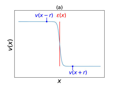
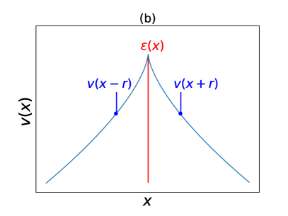
Figure 1: (a) Schematic depiction of a shock in Burgers turbulence. The local energy dissipation rate is peaked at the center of the shock $\varepsilon(x)$. Depending on the strength of the shock, the velocity field at $v(x-r)$ and at $v(x+r)$ possesses the symmetry $v(x-r)=-v(x+r)$, which leads to Burgers scaling (55). (b) In the case of cusplike structures, $\varepsilon(x)$ is still peaked in the center of the cusp. The symmetry of the cusps, however, leads to the vanishing of the dissipation anomaly in Eq. (52).

In the general case, i.e., for $n\neq 3$, we start by discarding the forcing contribution in the inertial range $\eta\ll r\ll L$ in assuming that $\chi(r)$ decreases sufficiently fast for increasing $r$. Moreover, in the limit of high Reynolds numbers, i.e., $\nu\rightarrow 0$, the smooth subleading viscous term $2\nu\frac{\partial^{2}}{\partial x^{2}}\langle(\delta_{r}v)^{n-1}\rangle$ can be neglected. Hence, in the inertial range where $\left\langle(\delta_{r}v)^{n-3}\right\rangle$ should admit scaling, we obtain

$$\left\langle\varepsilon(x)[\delta_{r}v(x)]^{n}\right\rangle\sim|r|^{\zeta(n+3)-1},$$ (54)

which agrees with the first result (9) of the MF model.

Hence, the prediction made by the MF model (9) becomes exact for the case of Burgers turbulence. It must be stressed that (52) does not further specify the scaling exponent $\zeta(n)$. It is well known that in order to go beyond it, we need some heuristic arguments about the dissipative term based on the geometrical structures of the flow. In high-Reynolds-number Burgers turbulence, we are faced with shocklike structures similar to the one in Fig. 1(a). In this case, the local energy dissipation rate is peaked at the center of the shock and the velocities $v(x+r)$ and $v(x-r)$ are arranged antisymmetrically around $v(x)=0$. In the limit of small viscosities and for small $r$, $v(x\pm r)$ possesses a negligible dependence on $r$ and we obtain

$$\big{\langle}\varepsilon(x)\{[\underbrace{\delta_{r}v(x)}_{=v(x+r)}]^{n-3}+[\underbrace{-\delta_{-r}v(x)}_{=-v(x-r)}]^{n-3}\}\big{\rangle}$$ (55)

$$\sim \langle v^{2}\rangle^{(n-3)/2}\langle\varepsilon\rangle\sim r^{\zeta(n)-1}\quad\rightarrow\quad\zeta(n)=1\;.$$

This is exactly the celebrated Burgers shock scaling from Table 1. It is important to stress that there exists a series of rigorous and quasirigorous results on the PDF of the gradient statistics in Burgers equations Chekhlov and Yakhot (1995); Yakhot and Chekhlov (1996); Polyakov (1995); Boldyrev (1997, 1998); Kraichnan (1957); Balkovsky et al. (1997); Chernykh and Stepanov (2001); E et al. (1997); E and Vanden Eijnden (1999, 2000). It is generally believed that it develops power-law tails in the inviscid limits. In our derivation, we do not pretend to control leading and sub-leading contributions in the zero-viscosity case. Our treatment is limited to estimate the regime of high but finite Reynolds number.

The influence of smooth velocity field structures can be seen as follows: Consider Eq. (52) for small $r$, in which case we can neglect the nonlinear and forcing contributions.

$$2\nu\frac{\partial^{2}}{\partial r^{2}}\langle[\delta_{r}v(x)]^{n-1}\rangle$$ (56)

$$\approx \frac{(n-1)(n-2)}{2}\left\langle\varepsilon(x)\{[\delta_{r}v(x)]^{n-3}+[-\delta_{-r}v(x)]^{n-3}\}\right\rangle$$

$$\approx 2\nu(n-1)(n-2)\left\langle\left(\frac{\partial v(x)}{\partial x}\right)^{n-1}r^{n-3}\right\rangle\;,$$

where we performed a Taylor expansion $\delta_{r}v(x)=v(x+r)-v(x)\approx\frac{\partial v(x)}{\partial x}r$ inside the ensemble average on the right-hand side and replaced the local energy dissipation rate $\varepsilon(x)$ with its definition (46). Integrating Eq. (56) and reinserting the definition of the local energy dissipation rate (46) yields

$$\langle[\delta_{r}v(x)]^{n}\rangle=2^{-n/2-1/2}\frac{\langle\varepsilon^{n/2}\rangle}{\nu^{n/2-1/2}}r^{n}.$$ (57)

Obviously, this result bears the signature of smooth ramp like velocity field contributions $v(x)$ in between shocks and is the leading term for $n<1$. Hence, by including the heuristic result (55), we obtain the well-known Burgers scaling

$$\langle|\delta_{r}v|^{n}\rangle\sim\begin{cases}\,r^{n}&\textrm{ for }n<1\\ \,r&\textrm{ for }n\geq 1\,.\end{cases}$$ (58)

In order to understand the importance of the exact shape of the singularity, it is instructive to consider the case of the Burgers equation with an additional nonlocality Zikanov et al. (1997); Friedrich and Grauer (2016).

$$\frac{\partial}{\partial t}v(x,t)+w(x,t)\frac{\partial}{\partial x}v(x,t)=\nu\frac{\partial^{2}}{\partial x^{2}}v(x,t)+F(x,t),$$ (59)

where the convective velocity field is given by

$$w(x,t)=\alpha v(x,t)+(1-\alpha)\textrm{P.V.}\int\textrm{d}x^{\prime}\frac{v(x^{\prime},t)}{x-x^{\prime}}~{},$$ (60)

where P.V. denotes principal value. Here $\alpha=1$ corresponds to the case of Burgers turbulence, whereas $\alpha=0$ corresponds to the purely nonlocal case that exhibits self-similar behavior Zikanov et al. (1997). In the latter case, the velocity field is dominated by cusplike structures similar to the one depicted in Fig. 1(b). Consequently, the velocity field possesses the symmetry $v(x-r)=v(x+r)$ leading to the vanishing of the dissipative term $\left\langle\varepsilon(x)\{[\delta_{r}v(x)]^{n-3}+[-\delta_{-r}v(x)]^{n-3}\}\right\rangle$ for even $n$. Furthermore, the nonlinear terms in the PDF hierarchy are changed due to the presence of the nonlocality in the generalized Burgers equation (59) and are necessarily unclosed Friedrich (2017). Accordingly, the nonlinear terms in the purely nonlocal case are balanced by the forcing terms. Depending on the properties of the forcing correlation function this scaling can be associated with the results of the renormalization group (see McComb (1990) for further references) and necessarily implies non-intermittent scaling.

Another important case of Eq. (52) is when the local dissipation rate and the velocity increment are statistically independent

$$\left\langle\varepsilon(x)\{[\delta_{r}v(x)]^{n-3}+[-\delta_{-r}v(x)]^{n-3}\}\right\rangle$$

$$=\underbrace{\left\langle\{[\delta_{r}v(x)]^{n-3}+[-\delta_{-r}v(x)]^{n-3}\}\right\rangle}_{\sim r_{1}^{\zeta(n-3)}}\left\langle\varepsilon(x)\right\rangle$$

$$\sim r^{\zeta(n)-1}\rightarrow\;\zeta(n)-1=\zeta(n-3)\;\rightarrow\;\zeta(n)=n/3.$$

which necessarily implies Kolmogorov (K41) scaling. The case of Burgers scaling (55) must be considered as the opposite case: The energy dissipation rate is fully correlated with the velocity increment, leading to strong intermittency. Furthermore, it has been shown that the intermediate case $0<\alpha<1$ in Eq. (59) shares many resemblances with the original Navier-Stokes equation Zikanov et al. (1997); Friedrich and Grauer (2016). Accordingly, the pressure must have a regularizing effect on the velocity field structures that enter the dissipation anomaly.

In the following section, we will evaluate both the fusion rules from Sec. III and the multifractal prediction from direct numerical simulations of Burgers turbulence.

IV.2 Direct numerical simulations of Burgers turbulence

In order to validate the theoretical considerations of the previous sections, we performed direct numerical simulations (DNSs) of the stochastically driven Burgers equation (47). The numerical setup consists of a second order Adams-Bashforth explicit solver paired with an Euler-Maruyama step to account for the large-scale Gaussian random forcing. We also consider the variable transformation $\hat{v}^{\prime}_{k}(t)=\exp(-\nu\,k^{2}\,dt)\hat{v}_{k}(t)$, which implies the exact integration of the viscous term. It relaxes the restriction on the time step by the diffusive term and significantly improves the convergence for large wave numbers. The spatial correlation function of the forcing (48) follows a power law proportional to $k^{-2}$ in Fourier space and has a cutoff at $k_{F}=5$. Table 2 contains a list of the characteristic parameters in use for the simulations presented in Figs. 3–5. The resolution was fixed such that $\eta/\textrm{d}x\approx 6$ at the highest Reynolds number. To improve the statistics we averaged over 200 independent runs.

Table 2: Characteristic parameters of the numerical simulations: root-mean-square velocity $v_{\rm rms}=\sqrt{\langle v^{2}\rangle}$, viscosity $\nu$, averaged rate of local energy dissipation $\langle\varepsilon\rangle=2\nu\left\langle\left(\frac{\partial v}{\partial x}\right)^{2}\right\rangle$, grid spacing $dx$, timestep $dt$, dissipation length $\eta=\left(\frac{\nu^{3}}{\langle\varepsilon\rangle}\right)^{1/4}$, Taylor length $\lambda=v_{\rm rms}\sqrt{\frac{2\nu}{\langle\varepsilon\rangle}}$, Taylor-Reynolds number $\textrm{Re}_{\lambda}=\frac{v_{\rm rms}\lambda}{\nu}$, integral length scale $L=\frac{E_{\rm kin}^{3/2}}{\langle\varepsilon\rangle}$, kinetic energy $E_{\rm kin}=\frac{1}{2}v_{\rm rms}^{2}$, large-eddy turnover time $T_{L}=\frac{L}{v_{\rm rms}}$, number of grid points $N$, and maximum force wavenumber of the power-law forcing $k_{F}$. The physical domain size is $2\pi$.

Parameter	Run 1	Run 2	Run 3
$u_{\rm rms}$	1.16	1.16	1.15
$\nu$	$3.6\times 10^{-4}$	$1.2\times 10^{-3}$	$6.8\times 10^{-3}$
Re	1800	550	90
Reλ	100	56	23
$\langle\varepsilon\rangle$	1	1	1
$dt$	$1.53\times 10^{-5}$	$1.53\times 10^{-5}$	$1.53\cdot 10^{-5}$
$dx$	$3.83\times 10^{-4}$	$3.83\times 10^{-4}$	$3.83\cdot 10^{-4}$
$\eta$	$2.61\times 10^{-3}$	$6.31\times 10^{-3}$	$2.37\times 10^{-2}$
$\lambda$	0.031	0.056	0.134
$L$	1.564	1.555	1.526
$T$ in $T_{L}$	760	762	772
$N$	$2^{14}$	$2^{14}$	$2^{14}$
$k_{F}$	5	5	5

IV.2.1 Evaluation of inertial-inertial fusion rules from DNS of Burgers turbulence

First, we investigate the validity of the fusion rules (4) for the Burgers equation. To this end, we consider the quantity

$$F_{p,q}(r,R)=\langle(\delta_{r}v)^{p}(\delta_{R}v)^{q}\rangle\;.$$ (62)

The application of the fusion rules (4) in conjunction with the Burgers scaling (58) yields three different possible scaling properties, depending on the order of the moments $p$ and $q$. If both increments are dominated by the shock we have case I, if both are dominated by the smooth ramps we have the case II, and if the small scale is smooth and the large scale is dominated by the shock we have case III. The scaling prediction in the plane $(p,q)$ is summarized in Fig. 2 and as follows:

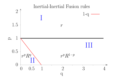
Figure 2: Parametric space of the exponents of Eq. (62) and the corresponding fusion rule prediction. Here I–III correspond to the three regions that emerge from the bifractal Burgers scaling (58).

$$F_{p,q}(r,R)\sim\begin{cases}\,r&\text{for $p>1$}\\ \,r^{p}\,R^{q}&\text{for $p<1$ \& $p+q\leq 1$}\\ \,r^{p}\,R^{1-p}&\text{for $p<1$ \& $p+q\geq 1$}\,.\end{cases}$$ (63)

In the following, we set the large scale $R$ equal to $\pi/2$ and vary the small scale $r$. The large scale $R$ is fixed so that $R/\eta\approx 600$ for $\textrm{Re}=1800$, $R/\eta\approx 250$ for $\textrm{Re}=550$, and $R/\eta\approx 70$ for $\textrm{Re}=90$. We have also tested the opposite scenario by fixing the small scale $r$ to $\alpha\eta$ with $\alpha\in[2,10]$, which yielded similar results that will therefore not be shown here. Figure 3 depicts $F_{p,q}(r,R)$ for three values in the three regions of Fig. 2: ($p=2,q=4$) [Fig. 3(a), region I], ($p=q=0.4$) [Fig. 3(b), region II], and ($p=0.6,q=2$) [Fig. 3(c), region III]. As one can see, all three cases agree fairly well with the theoretical predictions (black lines with the corresponding predicted scaling). This becomes even more apparent from the insets in Fig. 3, which shows $F_{p,q}(r,R)$ compensated by the corresponding prediction. We observe constant ($r$-independent) regions over a few decades of $r/R$. However, as $r$ approaches larger values and tends towards $R$, the compensated function becomes $r$-dependent, which indicates a breakdown of the fusion rules for small-scale separations. As discussed in Sec. III, the breakdown of the fusion rules for small-scale separations can also be interpreted in terms of the violation of the Markov property (28). In the following section, we will consider the special case of $F(r,R)$ for $r\rightarrow\eta$ to check the viscous-inertial scaling.

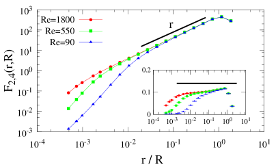
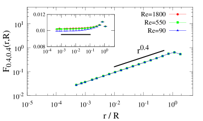
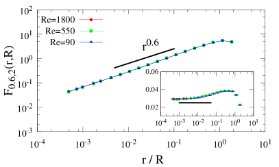
Figure 3: Examination of the inertial-inertial fusion rules (63) for runs 1–3 via the quantity $F_{p,q}(r,R)$ defined in Eq. (62) as a function of $r/R$ for different values of $p$ and $q$ and for different Reynolds numbers: (a) $p=2$ and $q=4$ (region I). (b) $p=q=0.4$ (region II). (c) $p=0.6$ and $q=2$ (region III). The black line corresponds to the fusion-rule prediction in Burgers turbulence summarized in the three regions I–III of Fig. 2. The inset depicts $F_{p,q}(r,R)$ divided by this prediction.

IV.2.2 Evaluation of the viscous-inertial fusion rules prediction from DNS of Burgers turbulence

In the following, we consider the viscous-inertial multiscale correlation function given

$$D_{p,q}(\textrm{Re},R)=\langle(\partial_{x}v)^{p}(\delta_{R}v)^{q}\rangle.$$ (64)

We specialize to the Burgers case for which the MF prediction is given in Fig. 4 and as follows by inspecting Eq. (17):

$$D_{p,q}(\textrm{Re},R)\sim\begin{cases}\,\textrm{Re}^{p-1}&\text{for $p>1$}\,,\\ \,R^{q}&\text{for $p<1$ \& $p+q\leq 1$}\,,\\ \,R^{1-p}&\text{for $p<1$ \& $p+q\geq 1$}\,.\end{cases}$$ (65)

In the following, we will also refer to these relations as the MF prediction for the viscous-inertial fusion rules.

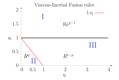
Figure 4: Parametric space of the exponents of Eq. (64) and the MF prediction for the viscous-inertial fusion rules. Here I–III correspond to the three regions that emerge from the bifractal Burgers scaling (58).

Figure 5(a) depicts $\nu D_{2,4}(\textrm{Re},R)$ as a function of $R$ for different Reynolds numbers (see also Table 2). As can be seen, $\nu D_{2,4}(\textrm{Re},R)$ is independent of the scale $R$ in the inertial range, which is in accordance with the MF prediction in region I of Fig. 4. The collapse of the data comes in agreement with the existence of a generalized dissipative anomaly as discussed in Sec. II and Eq. (9). The flat region increases as $\nu\rightarrow 0$. Figures 5(b) and  5(c) depict $D_{0.4,0.4}(\textrm{Re},R)$ and $D_{0.6,2}(\textrm{Re},R)$ respectively, with combinations of exponents $p$ and $q$ corresponding to regions II and III of Fig. 4, accordingly. The black line with scaling $R^{m}$, $m\in\mathbb{R}$, is the viscous-inertial fusion rules prediction following Eq. (65) for the chosen exponents $p$ and $q$. The inset depicts the data divided by $R^{m}$. All three cases show a good agreement of the data with the viscous-inertial fusion rules prediction, which improves as we increase Re.

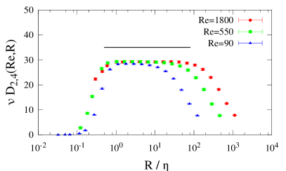
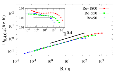
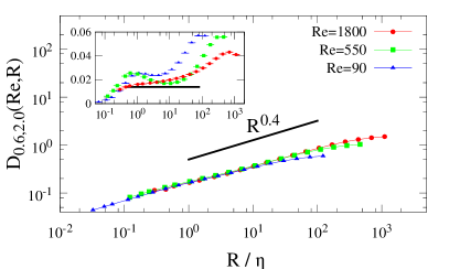
Figure 5: Examination of the viscous-inertial fusion rules prediction (65) via the quantity $D_{p,q}(\textrm{Re},R)$ defined in Eq. (64) as a function of $R/\eta$ for different values of $p$ and $q$ and for different Reynolds numbers. The insets depict the results divided by the corresponding viscous-inertial fusion rules prediction of regions I-III of Fig. 4. (a) $p=2$ and $q=4$ (region I). The quantity $\nu\,D_{2,4}(\textrm{Re},R)$ is shown here. It is independent of $R$, and the collapse of the data within errorbars supports the suggestion of a generalized dissipative anomaly discussed in Sec. II and Eq. (9). (b) $p=q=0.4$ (region II). (c) $p=0.6$ and $q=2$ (region III).

IV.2.3 Evaluation of the velocity gradient statistics from DNS of Burgers turbulence

Finally, we want to consider the special case where Eq. (64) reduces to the ordinary moments of the velocity gradient, i.e., $D_{p,0}(\textrm{Re})$. As can be seen from Fig. 4, the MF prediction for Burgers turbulence reduces to the Reynolds number scaling

$$D_{p,0}\sim\textrm{Re}^{p-1}\qquad\textrm{for $p>1$}\;.$$ (66)

Moreover, for the particular case of Burgers turbulence with $\zeta(n)=1$, both the MF prediction (17) and the result from Yakhot (2001); Yakhot and Sreenivasan (2004); Schumacher et al. (2007) in Eq. (23) yield the relation (66), which was already discussed in Sec. II. It is convenient to introduce the quantity

$$M_{p}=\frac{\left\langle\left(\frac{\partial v}{\partial x}\right)^{p}\right\rangle}{\left\langle\left(\frac{\partial v}{\partial x}\right)^{2}\right\rangle^{p/2}}$$ (67)

for even $p$. Recent numerical investigations of hydrodynamic turbulence Yakhot and Donzis (2017) suggest that the moments (67) exhibit a transition from Gaussian to anomalous behavior if one increases the Reynolds number. Hence, we expect $M_{p}$ to behave according to

$$M_{p}\sim\begin{cases}\,(p-1)!!&\textrm{ for}\;\textrm{Re}\sim O(1)\;,\\ \,\textrm{Re}^{p/2-1}\sim\textrm{Re}_{\lambda}^{p-2}&\textrm{ for }\textrm{Re}\gg O(1)\end{cases}$$ (68)

for even $p$. Here we made use of the fact that the Taylor-Reynolds number $\textrm{Re}_{\lambda}=u_{\rm rms}\lambda/\nu$ is related to Re according to $\textrm{Re}\sim\textrm{Re}_{\lambda}^{2}$ in the high-Reynolds-number regime.

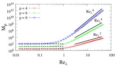
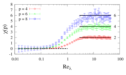
Figure 6: (a) Moments $M_{p}$ from Eq. (67) as a function of the Taylor-Reynolds number in Burgers turbulence. The low-Reynolds-number regime exhibits Gaussian statistics (dashed black lines), whereas the high-Reynolds-number regime agrees well with the multifractal prediction (17) and the result from Yakhot (2001); Yakhot and Sreenivasan (2004); Schumacher et al. (2007) (solid black line) for Burgers turbulence (68). The lines correspond to flat regions of the logarithmic derivative of the moments $\chi(n)$ [see (b)]. (b) Logarithmic derivative of the moments (69). The straight black lines correspond to the theoretical predictions (68), $\chi(4)=2$, $\chi(6)=4$, and $\chi(8)=6$.

Figure  6 is in quantitative agreement with Eq. (68). Figure  6(a) depicts the moments (67) as a function of the Taylor-Reynolds number. For small $\textrm{Re}_{\lambda}$, the moments exhibit Gaussian statistics similar to the case of hydrodynamic turbulence Yakhot and Donzis (2017), whereas the anomalous behavior for larger $\textrm{Re}_{\lambda}$ is much more pronounced in comparison to the latter case. Obviously, this result can be attributed to the strong intermittency behavior in Burgers turbulence. Nevertheless, in the high-Reynolds-number regime we can confirm the prediction (68) to a great extent. The fits (black lines) in Fig. 6(a) correspond to flat regions in the logarithmic derivative of the moments (67)

$$\chi(p)=\frac{\textrm{d}\log M_{p}}{\textrm{d}\log\textrm{Re}_{\lambda}},$$ (69)

which is displayed in Fig. 6(b). The flat regions are indicated as flat lines which correspond to the theoretical predictions (68), $\chi(4)=2$, $\chi(6)=4$, and $\chi(8)=6$. Hence, we can conclude that the MF prediction also applies to the single-gradient statistics in Burgers turbulence.

V Conclusion

We have presented an overview of prevalent concepts that allow for multiscale descriptions of turbulent flows. A main result of this paper is that the operator-product-expansion–fusion-rules approach Eyink (1993); Polyakov (1995); L’vov and Procaccia (1996a, b) that emanated from quantum field theory is a direct consequence of the Markov property of velocity increments in scale devised in Friedrich and Peinke (1997), provided that the structure functions exhibit scaling in the inertial range. This means an amalgamation of two fields that co-existed for nearly 20 years. By contrast, our results might also lead to a novel stochastic interpretation of the operator-product expansion in quantum field theory Wilson (1969). Different from other closure methods, e.g., the quasinormal approximation Millionschikov (1941), renormalization methods Kraichnan (1957); Wyld (1961), renormalization-group methods Forster et al. (1977), and the eddy-damped quasinormal approximation Orszag (1970, 1974); McComb (1990); Lesieur (2012), both the Markov approach and the operator-product expansion are nonperturbative, i.e., are not based on properties of Gaussian-distributed velocity field fluctuations. The latter property makes both approaches suitable candidates for a closure of the multi-increment PDF hierarchy Friedrich (2017).

Regarding the breakdown of the fusion rules in the limit of small-scale separations, it is tempting to investigate the influence of non-Markovian cascade processes. Here, a generalization of the KM expansion for the transition PDF (31) to arbitrary stochastic processes as emphasized in Srinivas and Wolf (1977), might yield a generalization of the fusion rules to arbitrary cascade processes. A dissipative cutoff of the structure functions Meneveau (1996) can also be achieved by a dissipative KM expansion, but is beyond the scope of the present work. In addition, the Markov property could be considered as a first step in an approximation of multi-increment statistics. The natural next step would be an extension incorporating one additional level of memory in scale Friedrich (2017), e.g., assuming

$$p(v_{4},r_{4}|v_{3},r_{3};v_{2},r_{2};v_{1},r_{1})\approx p(v_{4},r_{4}|v_{3},r_{3};v_{2},r_{2})\;,$$ (70)

and thus allowing one to capture correlations between the inertial and viscous-inertial ranges.

Furthermore, we have shown that a specific prediction of the MF model for joint velocity gradient and velocity increment statistics (9) can be obtained from the basic fluid dynamical equations under the neglect of pressure contributions, i.e., from the Burgers equation. It must be stressed that this result can be derived without any further assumptions apart from the scaling of structure functions in the inertial range. However, at this point, we could not validate the generalization of the MF result to arbitrary powers of the velocity gradient given by Eq. (13). In order to derive such a generalization, one has to operate at the next level of the multi-increment hierarchy (50). Here a possible closure is the Markov property (28) which, leads to a self-consistent equation for the two-increment PDF Friedrich (2017).

The numerical part of this work was devoted to the verification of fusion rules and the prediction of the MF prediction in DNSs of Burgers turbulence. Both fusion rules and MF prediction could be established to a certain extent. The limitation of the fusion rules arises for vanishing scale separations and could be understood from the violation of the Markov property (28). A further examination of this regime is a task left to future research.

VI Acknowledgement

J.F. and R.G. acknowledge fruitful discussions with J. Schumacher and J. Peinke. L.B. acknowledges funding from the European Research Council under the European Union’s Seventh Framework Programme, ERC Grant Agreement No. 339032. G.M. kindly acknowledges funding from the European Union’s Horizon 2020 research and innovation program under the Marie Skłodowska-Curie Grant Agreement No. 642069 (European Joint Doctorate program “HPC-LEAP”).

Appendix A Generalization of fusion rules to $n$-increment statistics

We consider the moments of the $n$-increment PDF

$$\left\langle(\delta_{r_{n}}v)^{p_{n}}\cdots(\delta_{r_{2}}v)^{p_{2}}(\delta_{r_{1}}v)^{p_{1}}\right\rangle$$

$$= \int\textrm{d}v_{n}\cdots\textrm{d}v_{2}\;\textrm{d}v_{1}\;v_{n}^{p_{n}}\cdots v_{2}^{p_{2}}\;v_{1}^{p_{1}}\;f_{n}(v_{n},r_{n};\cdots;v_{1},r_{1})\;,$$

where the $p_{i}$’s denote arbitrary exponents and we impose the scale ordering $\eta\leq r_{n}\leq r_{n-1}\leq\ldots\leq r_{2}\leq r_{1}\leq L$. First, we rewrite the $n$-increment PDF according to Bayes’ theorem

$$f_{n}(v_{n},r_{n};\ldots v_{1},r_{1})$$ (72)

$$= p(v_{n},r_{n}|v_{n-1},r_{n-1};\ldots;v_{1},r_{1})$$

$$\times f_{n-1}(v_{n-1},r_{n-1};\ldots v_{1},r_{1}).$$

The general form of the Markov property in scale implies that

$$p(v_{n},r_{n}|v_{n-1},r_{n-1};\ldots;v_{1},r_{1})=p(v_{n},r_{n}|v_{n-1},r_{n-1})\;.$$ (73)

Hence, Eq. (A) simplifies to

$$\int\textrm{d}v_{n}\ldots\textrm{d}v_{2}\;\textrm{d}v_{1}\;v_{n}^{p_{n}}\ldots v_{2}^{p_{2}}\;v_{1}^{p_{1}}\;p(v_{n},r_{n}|v_{n-1},r_{n-1})$$ (74)

$$\times f_{n-1}(v_{n-1},r_{n-1};\ldots;v_{1},r_{1})$$

Under the assumption of the scaling of structure functions in combination with the Markov property, we can express the conditional probability $p(v_{n},r_{n}|v_{n-1},r_{n-1})$ in terms of a Dyson series (39)

$$p(v_{n},r_{n}|v_{n-1},r_{n-1}) = \delta(v_{n}-v_{n-1})+\ln\frac{r_{n-1}}{r_{n}}\sum_{k=1}^{\infty}\frac{K_{k}}{k!}\frac{\partial^{k}}{\partial v_{n}^{k}}v_{n}^{k}\delta(v_{n}-v_{n-1})$$ (75)

$$+\frac{1}{2!}\left(\ln\frac{r_{n-1}}{r_{n}}\right)^{2}\sum_{k=1}^{\infty}\frac{K_{k}}{k!}\frac{\partial^{k}}{\partial v_{n}^{k}}v_{n}^{k}\sum_{l=1}^{\infty}\frac{K_{l}}{l!}\frac{\partial^{l}}{\partial v_{n}^{l}}v_{n}^{l}\delta(v_{n}-v_{n-1})+\cdots$$

Inserting (75) into (74) and performing the partial integrations with respect to $v_{n}$ similar to Eq. (43) yields

$$\left[1+\sum_{k=1}^{p_{n}}(-1)^{k}K_{k}{p_{n}\choose k}\ln\frac{r_{n-1}}{r_{n}}+\frac{1}{2!}\sum_{k=1}^{p_{n}}(-1)^{k}K_{k}{p_{n}\choose k}\sum_{l=1}^{p_{n}}(-1)^{l}K_{l}{p_{n}\choose l}\left(\ln\frac{r_{n-1}}{r_{n}}\right)^{2}+\ldots\right]$$

$$\times\int\textrm{d}v_{n-1}\ldots\textrm{d}v_{2}\;\textrm{d}v_{1}\;v_{n-1}^{p_{n}+p_{n-1}}\ldots v_{2}^{p_{2}}\;v_{1}^{p_{1}}\;f_{n-1}(v_{n-1},r_{n-1};\ldots;v_{1},r_{1})\;.$$

Here the term in square brackets can be written as an exponential function according to

$$\Big{[}\ldots\Big{]}=\exp\left[\ln\frac{r_{n-1}}{r_{n}}\sum_{k=1}^{p_{n}}(-1)^{k}K_{k}{p_{n}\choose k}\right]\;.$$ (77)

The sum in the exponential function can be identified as the scaling exponent $\zeta(p_{n})=-\sum_{k=1}^{p_{n}}(-1)^{k}K_{k}{p_{n}\choose k}$ and we obtain

$$\left\langle(\delta_{r_{n}}v)^{p_{n}}(\delta_{r_{n-1}}v)^{p_{n-1}}\cdots(\delta_{r_{2}}v)^{p_{2}}(\delta_{r_{1}}v)^{p_{1}}\right\rangle$$ (78)

$$= \exp\left[\ln\frac{r_{n}}{r_{n-1}}\zeta(p_{n})\right]$$

$$\times\left\langle(\delta_{r_{n-1}}v)^{p_{n}+p_{n-1}}\cdots(\delta_{r_{2}}v)^{p_{2}}(\delta_{r_{1}}v)^{p_{1}}\right\rangle.$$

Furthermore, the scaling of the structure functions implies that $\left\langle(\delta_{r_{n}}v)^{p_{n}}\right\rangle\sim r_{n}^{\zeta(p_{n})}$, which yields

$$\left\langle(\delta_{r_{n}}v)^{p_{n}}(\delta_{r_{n-1}}v)^{p_{n-1}}\cdots(\delta_{r_{2}}v)^{p_{2}}(\delta_{r_{1}}v)^{p_{1}}\right\rangle$$

$$= \frac{\left\langle(\delta_{r_{n}}v)^{p_{n}}\right\rangle}{\left\langle(\delta_{r_{n-1}}v)^{p_{n}}\right\rangle}\left\langle(\delta_{r_{n-1}}v)^{p_{n}+p_{n-1}}\cdots(\delta_{r_{2}}v)^{p_{2}}(\delta_{r_{1}}v)^{p_{1}}\right\rangle\;.$$

Successive application of this relation yields

$$\left\langle(\delta_{r_{n}}v)^{p_{n}}(\delta_{r_{n-1}}v)^{p_{n-1}}\ldots(\delta_{r_{2}}v)^{p_{2}}(\delta_{r_{1}}v)^{p_{1}}\right\rangle$$ (80)

$$= \frac{\left\langle(\delta_{r_{n}}v)^{p_{n}}\right\rangle}{\left\langle(\delta_{r_{n-1}}v)^{p_{n}}\right\rangle}\times\frac{\langle\left(\delta_{r_{n-1}}v)^{p_{n}+p_{n-1}}\right\rangle}{\left\langle(\delta_{r_{n-2}}v)^{p_{n}+p_{n-1}}\right\rangle}\times\cdots$$

$$\times\frac{\left\langle(\delta_{r_{2}}v)^{p_{n}+\cdots+p_{2}}\right\rangle}{\left\langle(\delta_{r_{1}}v)^{p_{n}+\cdots+p_{2}}\right\rangle}\times\left\langle(\delta_{r_{1}}v)^{p_{n}+\cdots+p_{1}}\right\rangle\;,$$

or in more compact notation

$$\prod_{i=1}^{n}\left\langle(\delta_{r_{i}}v)^{p_{i}}\right\rangle$$

$$= \prod_{i=1}^{n-1}\frac{\left\langle(\delta_{r_{i+1}}v)^{\sum_{k=1}^{i}p_{n+1-k}}\right\rangle}{\left\langle(\delta_{r_{i}}v)^{\sum_{k=1}^{i}p_{n+1-k}}\right\rangle}\left\langle(\delta_{r_{1}}v)^{\sum_{k=1}^{n}p_{n+1-k}}\right\rangle\;,$$

which is the counterpart to Eq. (III).

Appendix B Derivation of multi-increment hierarchy in Burgers turbulence

In order to derive the evolution equation (50) we take the temporal derivative of the one-increment PDF

$$\frac{\partial}{\partial t}f_{1}(v_{1},r_{1},t)=\frac{\partial}{\partial t}\langle\delta(v_{1}-\delta_{r_{1}}v(x,t))\rangle=-\frac{\partial}{\partial v_{1}}\left\langle\delta(v_{1}-\delta_{r_{1}}v(x,t))\frac{\partial}{\partial t}\delta_{r_{1}}v(x,t)\right\rangle$$

$$= \frac{\partial}{\partial v_{1}}\left\langle\delta(v_{1}-\delta_{r_{1}}v(x,t))\left[v(x,t)\frac{\partial}{\partial x}\delta_{r_{1}}v(x,t)+\delta_{r_{1}}v(x,t)\frac{\partial}{\partial r_{1}}\delta_{r_{1}}v(x,t)-\nu\frac{\partial^{2}}{\partial x^{2}}\delta_{r_{1}}v(x,t)-F(x+r_{1},t)+F(x,t)\right]\right\rangle,$$

where Eq. (49) was used in order to replace the temporal evolution of the velocity increment. Each term can now be treated separately. Starting with the first advective term, we obtain

$$- \frac{\partial}{\partial v_{1}}\left\langle\delta(v_{1}-\delta_{r_{1}}v(x,t))v(x,t)\frac{\partial}{\partial x}\delta_{r_{1}}v(x,t)\right\rangle=\left\langle v(x,t)\frac{\partial}{\partial x}\delta(v_{1}-\delta_{r_{1}}v(x,t))\right\rangle=\underbrace{\frac{\partial}{\partial x}\left\langle v(x,t)\delta(v_{1}-\delta_{r_{1}}v(x,t))\right\rangle}_{=0,\;\textrm{homogeneity}}$$ (83)

$$-\left\langle\underbrace{\frac{\partial v(x,t)}{\partial x}\delta(v_{1}-\delta_{r_{1}}v(x,t))}_{=\left[\frac{\partial\delta_{r_{1}}v(x,t)}{\partial r_{1}}-\frac{\partial\delta_{r_{1}}v(x,t)}{\partial x}\right]\times\delta}\right\rangle=\int_{-\infty}^{v_{1}}\textrm{d}v_{1}^{\prime}\frac{\partial}{\partial r_{1}}\langle\underbrace{\delta(v_{1}^{\prime}-\delta_{r_{1}}v(x,t))\rangle}_{=f_{1}(v_{1}^{\prime},r,t)}-\int_{-\infty}^{v_{1}}\textrm{d}v_{1}^{\prime}\underbrace{\frac{\partial}{\partial x}\langle\delta(v_{1}^{\prime}-\delta_{r_{1}}v(x,t))\rangle}_{=0,\;\textrm{homogeneity}}\;.$$

Here we made use of the inverse chain rule in the first and last steps. The second advective term can be treated in the same way according to

$$-\frac{\partial}{\partial v_{1}}\left\langle\delta(v_{1}-\delta_{r_{1}}v(x,t))\delta_{r_{1}}v(x,t)\frac{\partial}{\partial r_{1}}\delta_{r_{1}}v(x,t)\right\rangle$$ (84)

$$= \left\langle\delta_{r_{1}}v(x,t)\frac{\partial}{\partial r_{1}}\delta(v_{1}-\delta_{r_{1}}v(x,t))\right\rangle=\frac{\partial}{\partial r_{1}}\left\langle\delta_{r_{1}}v(x,t)\delta(v_{1}-\delta_{r_{1}}v(x,t))\right\rangle-\left\langle\frac{\partial\delta_{r_{1}}v(x,t)}{\partial r_{1}}\delta(v_{1}-\delta_{r_{1}}v(x,t))\right\rangle$$

$$= v_{1}\frac{\partial}{\partial r_{1}}\underbrace{\left\langle\delta(v_{1}-\delta_{r_{1}}v(x,t))\right\rangle}_{=f_{1}(v_{1},r_{1},t)}+\int_{-\infty}^{v_{1}}\textrm{d}v_{1}^{\prime}\frac{\partial}{\partial r_{1}}\langle\underbrace{\delta(v_{1}^{\prime}-\delta_{r_{1}}v(x,t))\rangle}_{=f_{1}(v_{1}^{\prime},r_{1},t)},$$

where we made use of the sifting property of the $\delta$ function, i.e., $\delta_{r_{1}}v(x,t)\delta(v_{1}-\delta_{r_{1}}v(x,t))=v_{1}\delta(v_{1}-\delta_{r_{1}}v(x,t))$. The nonlinear terms can thus be expressed solely in terms of the one-increment PDF or its associated cumulative PDF. which is a particularity of the Burgers equation (for the Navier-Stokes equation we would be facing unclosed terms from the pressure Ulinich and Lyubimov (1969)). However, the viscous contributions in Eq. (B) confront us with unclosed terms and we have to introduce the two-increment PDF, which results in an infinite hierarchy of PDF equations. This can be seen from the calculation of the viscous term in Eq. (B),

$$- \nu\left\langle\delta(v_{1}-\delta_{r_{1}}v(x,t))\frac{\partial^{2}\delta_{r_{1}}v(x,t)}{\partial x^{2}}\right\rangle=-\nu\left\langle\delta(v_{1}-\delta_{r_{1}}v(x,t))\left[\frac{\partial^{2}\delta_{r_{1}}v(x,t)}{\partial r_{1}^{2}}-\frac{\partial^{2}v(x,t)}{\partial x^{2}}\right]\right\rangle$$ (85)

$$= -\nu\int\textrm{d}r_{2}\left[\delta(r_{2}-r_{1})-\delta(r_{2})\right]\frac{\partial^{2}}{\partial r_{2}^{2}}\left\langle\delta_{r_{2}}v(x,t)\delta(v_{1}-\delta_{r_{1}}v(x,t))\right\rangle$$

$$= -\nu\int\textrm{d}r_{2}\left[\delta(r_{2}-r_{1})-\delta(r_{2})\right]\frac{\partial^{2}}{\partial r_{2}^{2}}\int\textrm{d}v_{2}v_{2}\underbrace{\left\langle\delta(v_{2}-\delta_{r_{2}}v(x,t))\delta(v_{1}-\delta_{r_{1}}v(x,t))\right\rangle}_{=f_{2}(v_{2},r_{2};v_{1},r_{1},t)}.$$

The forcing contributions in Eq. (B) can be handled by the usual trick of the Langevin equation. Inserting the above calculations yields the evolution equation for the one-increment PDF

$$\frac{\partial}{\partial t}f_{1}(v_{1},r_{1},t)+v_{1}\frac{\partial}{\partial r_{1}}f_{1}(v_{1},r_{1},t)+2\int_{-\infty}^{v_{1}}\textrm{d}v_{1}^{\prime}\frac{\partial}{\partial r_{1}}f_{1}(v_{1}^{\prime},r_{1},t)$$ (86)

$$= -\nu\frac{\partial}{\partial v_{1}}\int\textrm{d}r_{2}\left[\delta(r_{2}-r_{1})-\delta(r_{2})\right]\frac{\partial^{2}}{\partial r_{2}^{2}}\int\textrm{d}v_{2}v_{2}f_{2}(v_{2},r_{2};v_{1},r_{1},t)+[\chi(0)-\chi(r_{1})]\frac{\partial^{2}}{\partial v_{1}^{2}}f_{1}(v,r_{1},t)\;.$$

Appendix C Reformulation of the viscous term in the multi-increment hierarchy

In this appendix, we show that the unclosed term in the evolution equation of the one-increment PDF (50) involves the local energy dissipation rate. To this end, we rewrite the viscous contributions in their original form according to

$$\nu \int\textrm{d}r_{2}\left[\delta(r_{2}-r_{1})-\delta(r_{2})\right]\frac{\partial^{2}}{\partial r_{2}^{2}}\int\textrm{d}v_{2}v_{2}f_{2}(v_{2},r_{2};v_{1},r_{1})$$ (87)

$$= \nu\left\langle\left[\frac{\partial^{2}\delta_{r_{1}}v(x)}{\partial r_{1}^{2}}-\frac{\partial^{2}u(x)}{\partial x^{2}}\right]\delta(v_{1}-\delta_{r_{1}}v(x))\right\rangle\;.$$

A further treatment of these terms yields

$$+\nu\frac{\partial}{\partial r_{1}}\left\langle\frac{\partial\delta_{r_{1}}v(x)}{\partial r_{1}}\delta(v_{1}-\delta_{r_{1}}v(x))\right\rangle-\nu\left\langle\frac{\partial\delta_{r_{1}}v(x)}{\partial r_{1}}\frac{\partial\delta(v_{1}-\delta_{r_{1}}v(x))}{\partial r_{1}}\right\rangle$$ (88)

$$-\nu\underbrace{\frac{\partial}{\partial x}\left\langle\frac{\partial v(x)}{\partial x}\delta(v_{1}-\delta_{r_{1}}v(x))\right\rangle}_{=0,~{}\textrm{homogeneity}}+\nu\left\langle\frac{\partial v(x)}{\partial x}\frac{\partial\delta(v_{1}-\delta_{r_{1}}v(x))}{\partial x}\right\rangle$$

$$= -\nu\int_{-\infty}^{v_{1}}\textrm{d}v_{1}^{\prime}\frac{\partial^{2}}{\partial r_{1}^{2}}\langle\delta(v_{1}^{\prime}-\delta_{r_{1}}v(x))\rangle+\nu\frac{\partial}{\partial v_{1}}\left\langle\left(\frac{\partial\delta_{r_{1}}v(x)}{\partial r_{1}}\right)^{2}\delta(v_{1}-\delta_{r_{1}}v(x))\right\rangle$$

$$-\nu\frac{\partial}{\partial v_{1}}\left\langle\frac{\partial v(x)}{\partial x}\underbrace{\left(\frac{\partial\delta_{r_{1}}v(x)}{\partial x}\right)}_{=\frac{\partial\delta_{r_{1}}v(x)}{\partial r_{1}}-\frac{\partial v(x)}{\partial x}}\delta(v_{1}-\delta_{r_{1}}v(x))\right\rangle.$$

Inserting the one-increment PDF $f_{1}(v_{1}^{\prime},r_{1})$ into the first term on the right-hand side yields

$$-\nu\int_{-\infty}^{v_{1}}\textrm{d}v_{1}^{\prime}\frac{\partial^{2}}{\partial r_{1}^{2}}f_{1}(v_{1}^{\prime},r_{1})+\nu\frac{\partial}{\partial v_{1}}\left\langle\left(\frac{\partial v(x+r_{1})}{\partial r_{1}}\right)^{2}\delta(v_{1}-\delta_{r_{1}}v(x))\right\rangle$$ (89)

$$+\nu\frac{\partial}{\partial x}\left\langle\underbrace{\left(\frac{\partial v(x)}{\partial x}\right)}_{=\frac{\partial\delta_{r_{1}}v(x)}{\partial r_{1}}-\frac{\partial\delta_{r_{1}}v(x)}{\partial x}}\delta(v_{1}-\delta_{r_{1}}v(x))\right\rangle+\nu\frac{\partial}{\partial v_{1}}\left\langle\left(\frac{\partial v(x)}{\partial x}\right)^{2}\delta(v_{1}-\delta_{r_{1}}v(x))\right\rangle$$

$$= -\nu\int_{-\infty}^{v_{1}}\textrm{d}v_{1}^{\prime}\frac{\partial^{2}}{\partial r_{1}^{2}}f_{1}(v_{1}^{\prime},r_{1})+\nu\frac{\partial}{\partial v_{1}}\left\langle\left(\frac{\partial v(x+r_{1})}{\partial r_{1}}\right)^{2}\delta(v_{1}-\delta_{r_{1}}v(x))\right\rangle$$

$$-\nu\int_{-\infty}^{v_{1}}\textrm{d}v_{1}^{\prime}\frac{\partial^{2}}{\partial r_{1}^{2}}f_{1}(v_{1}^{\prime},r)+\nu\int_{-\infty}^{v_{1}}\textrm{d}v_{1}^{\prime}\underbrace{\frac{\partial^{2}}{\partial r_{1}\partial x}f_{1}(v_{1}^{\prime},r_{1})}_{=0,~{}\textrm{homogeneity}}+\nu\frac{\partial}{\partial v_{1}}\left\langle\left(\frac{\partial v(x)}{\partial x}\right)^{2}\delta(v_{1}-\delta_{r_{1}}v(x))\right\rangle.$$

Under the assumption of homogeneity, we obtain

$$\left\langle\left(\frac{\partial v(x+r_{1})}{\partial r_{1}}\right)^{2}\delta(v_{1}-\delta_{r_{1}}v(x))\right\rangle$$ (90)

$$= \left\langle\left(\frac{\partial v(x+r_{1})}{\partial r_{1}}\right)^{2}\delta(v_{1}-v(x+r_{1})+v(x))\right\rangle$$

$$= \left\langle\left(\frac{\partial v(x)}{\partial x}\right)^{2}\delta(v_{1}-v(x)+v(x-r_{1}))\right\rangle$$

$$= \left\langle\left(\frac{\partial v(x)}{\partial x}\right)^{2}\delta(v_{1}+\delta_{-r_{1}}v(x))\right\rangle,$$

which allows us to introduce the local energy dissipation rate in Eq. (50) according to

$$v_{1}\frac{\partial}{\partial r_{1}}f_{1}(v_{1},r_{1})=2\int_{-\infty}^{v_{1}}\textrm{d}v_{1}^{\prime}\frac{\partial}{\partial r_{1}}f_{1}(v^{\prime},r_{1})$$ (91)

$$~{}-\frac{\partial^{2}}{\partial v_{1}^{2}}\Bigg{[}\left\langle\frac{\varepsilon(x)}{2}[\delta(v_{1}-\delta_{r_{1}}v(x))+\delta(v_{1}+\delta_{-r_{1}}v(x))]\right\rangle$$

$$+[\chi(0)-\chi(r_{1})]f_{1}(v_{1},r_{1})\Bigg{]}+2\nu\frac{\partial^{2}}{\partial r_{1}^{2}}f_{1}(v_{1},r_{1}).$$

References

• Frisch (1995) U. Frisch, Turbulence (Cambridge University Press, 1995).
• Monin and Yaglom (2007) A. S. Monin and A. M. Yaglom, Statistical Fluid Mechanics: Mechanics of Turbulence (Courier Dover Publications, 2007).
• Davidson (2015) P. Davidson, Turbulence: an introduction for scientists and engineers (Oxford University Press, USA, 2015).
• Wyngaard (2010) J. C. Wyngaard, Turbulence in the Atmosphere (Cambridge University Press, 2010).
• Pope (2001) S. B. Pope, “Turbulent flows,”  (2001).
• Parker (1979) E. N. Parker, Cosmical magnetic fields (The Clarendon Press, Oxford University Press, New York, 1979).
• Yakhot (2006) V. Yakhot, Physica D: Nonlinear Phenomena 215, 166 (2006).
• Ishihara et al. (2009) T. Ishihara, T. Gotoh,  and Y. Kaneda, Annual Review of Fluid Mechanics 41, 165 (2009).
• Benzi et al. (2010) R. Benzi, L. Biferale, R. Fisher, D. Lamb,  and F. Toschi, Journal of Fluid Mechanics 653, 221 (2010).
• Sinhuber et al. (2017) M. Sinhuber, G. P. Bewley,  and E. Bodenschatz, Physical review letters 119, 134502 (2017).
• Iyer et al. (2017) K. P. Iyer, K. R. Sreenivasan,  and P. Yeung, Phys. Rev. E 95, 021101 (2017).
• Reinke et al. (2017) N. Reinke, D. Nickelsen,  and J. Peinke, arXiv preprint arXiv:1702.03679  (2017).
• Bec and Khanin (2007) J. Bec and K. Khanin, Physics Reports 447, 1 (2007).
• Eyink (1993) G. L. Eyink, Phys. Lett. A 172, 355 (1993).
• L’vov and Procaccia (1996a) V. L’vov and I. Procaccia, Phys. Rev. Lett. 76, 2898 (1996a).
• L’vov and Procaccia (1996b) V. L’vov and I. Procaccia, Phys. Rev. E 54, 6268 (1996b).
• Benzi et al. (1998) R. Benzi, L. Biferale,  and F. Toschi, Phys. Rev. Lett. 80, 3244 (1998).
• Benzi et al. (1999) R. Benzi, L. Biferale, G. Ruiz-Chavarria, S. Ciliberto,  and F. Toschi, Phys. Fluids 11 (1999).
• Friedrich and Peinke (1997) R. Friedrich and J. Peinke, Phys. Rev. Lett. 78, 863 (1997).
• Friedrich and Grauer (2018) J. Friedrich and R. Grauer, in Complexity and Synergetics (Springer, 2018) pp. 39–49.
• Friedrich and Grauer (2016) J. Friedrich and R. Grauer, arXiv preprint arXiv:1610.04432  (2016).
• Friedrich (2017) J. Friedrich, Closure of the Lundgren-Monin-Novikov hierarchy in turbulence via a Markov property of velocity increments in scale, Ph.D. thesis, Ruhr-University Bochum (2017).
• Frisch and Vergassola (1991) U. Frisch and M. Vergassola, Europhys. Lett. 14, 439 (1991).
• Wilson (1969) K. G. Wilson, Phys. Rev. 179, 1499 (1969).
• Hill (2001) R. J. Hill, Journal of Fluid Mechanics 434, 379 (2001).
• Polyakov (1995) A. M. Polyakov, Phys. Rev. E 52, 6183 (1995).
• Duchon and Robert (2000) J. Duchon and R. Robert, Nonlinearity 13, 249 (2000).
• Risken (1996) H. Risken, The Fokker-Planck Equation (Springer, Berlin, 1996).
• Paladin and Vulpiani (1987) G. Paladin and A. Vulpiani, Phys. Rev. A 35, 1971 (1987).
• Nelkin (1990) M. Nelkin, Phys. Rev. A 42, 7226 (1990).
• Yakhot (2001) V. Yakhot, Phys. Rev. E 63, 26307 (2001).
• Yakhot and Sreenivasan (2004) V. Yakhot and K. R. Sreenivasan, Phys. A Stat. Mech. its Appl. 343, 147 (2004).
• Schumacher et al. (2007) J. Schumacher, K. R. Sreenivasan,  and V. Yakhot, New J. Phys. 9, 89 (2007).
• Benzi and Biferale (2009) R. Benzi and L. Biferale, J. Stat. Phys. 135, 977 (2009).
• Yeung et al. (2015) P. Yeung, X. Zhai,  and K. R. Sreenivasan, Proceedings of the National Academy of Sciences 112, 12633 (2015).
• Siefert and Peinke (2004) M. Siefert and J. Peinke, Phys. Rev. E 70, 015302 (2004).
• Stresing and Peinke (2010) R. Stresing and J. Peinke, New J. Phys. 12 (2010), 10.1088/1367-2630/12/10/103046.
• Nickelsen (2017) D. Nickelsen, Journal of Statistical Mechanics: Theory and Experiment , 073209, 22 (2017).
• Lück et al. (2006) S. Lück, C. Renner, J. Peinke,  and R. Friedrich, Phys. Lett. Sect. A Gen. At. Solid State Phys. 359, 335 (2006).
• Renner et al. (2001) C. Renner, J. Peinke,  and R. Friedrich, Journal of Fluid Mechanics 433, 383 (2001).
• Friedrich et al. (2011) R. Friedrich, J. Peinke, M. Sahimi,  and R. M. Tabar, Phys. Rep. 506, 87 (2011).
• Davoudi and Tabar (2000) J. Davoudi and M. R. R. Tabar, Phys. Rev. E 61, 6563 (2000).
• Eling and Oz (2015) C. Eling and Y. Oz, Journal of High Energy Physics 2015, 150 (2015).
• E and Vanden Eijnden (1999) W. E and E. Vanden Eijnden, Phys. Rev. Lett. 83, 2572 (1999).
• Chekhlov and Yakhot (1995) A. Chekhlov and V. Yakhot, Physical Review E 51, R2739 (1995).
• Yakhot and Chekhlov (1996) V. Yakhot and A. Chekhlov, Phys. Rev. Lett. 77, 3118 (1996).
• Boldyrev (1997) S. A. Boldyrev, Phys. Rev. E 55, 6907 (1997).
• Boldyrev (1998) S. A. Boldyrev, Physics of Plasmas 5, 1681 (1998)https://doi.org/10.1063/1.872836 .
• Kraichnan (1957) R. H. Kraichnan, Phys. Rev. 107, 1485 (1957).
• Balkovsky et al. (1997) E. Balkovsky, G. Falkovich, I. Kolokolov,  and V. Lebedev, Phys. Rev. Lett. 78, 1452 (1997).
• Chernykh and Stepanov (2001) A. I. Chernykh and M. G. Stepanov, Phys. Rev. E 64, 026306 (2001)arXiv:nlin/0001023 .
• et al. (1997) W. E, K. Khanin, A. Mazel,  and Y. Sinai, Phys. Rev. Lett. 78, 1904 (1997).
• E and Vanden Eijnden (2000) W. E and E. Vanden Eijnden, Communications on Pure and Applied Mathematics 53, 852 (2000).
• Zikanov et al. (1997) O. Zikanov, A. Thess,  and R. Grauer, Phys. Fluids 9, 1362 (1997).
• McComb (1990) W. D. McComb, The Physics of Fluid Turbulence (Oxford University Press, 1990).
• Yakhot and Donzis (2017) V. Yakhot and D. Donzis, Phys. Rev. Lett. 119, 044501 (2017).
• Millionschikov (1941) M. Millionschikov, Dokl. Akad. Nauk SSSR 32 (1941).
• Wyld (1961) H. W. Wyld, Ann. Phys. (N. Y). 14, 143 (1961).
• Forster et al. (1977) D. Forster, D. R. Nelson,  and M. J. Stephen, Phys. Rev. A 16, 732 (1977).
• Orszag (1970) S. A. Orszag, J. Fluid Mech. 41, 363 (1970).
• Orszag (1974) S. A. Orszag, Lectures on the statistical theory of turbulence (Flow Research Incorporated, 1974).
• Lesieur (2012) M. Lesieur, “Turbulence in Fluids,”  (2012).
• Srinivas and Wolf (1977) M. Srinivas and E. Wolf, in Statistical Mechanics and Statistical Methods in Theory and Application (Springer, 1977) pp. 219–252.
• Meneveau (1996) C. Meneveau, Phys. Rev. E 54, 3657 (1996).
• Ulinich and Lyubimov (1969) F. R. Ulinich and B. Y. Lyubimov, Sov. J. Exp. Theor. Phys. 28, 494 (1969).