Observations of a nearby filament of galaxy clusters with the Sardinia Radio Telescope

Abstract

We report the detection of diffuse radio emission which might be connected to a large-scale filament of the cosmic web covering a 8${}^{\circ}\times$8^∘ area in the sky, likely associated with a z$\approx$0.1 over-density traced by nine massive galaxy clusters. In this work, we present radio observations of this region taken with the Sardinia Radio Telescope. Two of the clusters in the field host a powerful radio halo sustained by violent ongoing mergers and provide direct proof of intra-cluster magnetic fields. In order to investigate the presence of large-scale diffuse radio synchrotron emission in and beyond the galaxy clusters in this complex system, we combined the data taken at 1.4 GHz obtained with the Sardinia Radio Telescope with higher resolution data taken with the NRAO VLA Sky Survey. We found 28 candidate new sources with a size larger and X-ray emission fainter than known diffuse large-scale synchrotron cluster sources for a given radio power. This new population is potentially the tip of the iceberg of a class of diffuse large-scale synchrotron sources associated with the filaments of the cosmic web. In addition, we found in the field a candidate new giant radio galaxy.

1 Introduction

One of the major challenges of the new generation of astronomical instruments is the detection of the magnetic cosmic web. According to cosmological simulations, half of the baryons expected in the Universe from the cosmic microwave background observations should be located in the filaments connecting galaxy clusters, in the form of a diffuse plasma (with median over-densities of about 10-30 and temperatures $10^{5}-10^{7}$ K, see Cen & Ostriker, 1999; Davé et al., 2001). Owing to the low density and intermediate temperature range, the thermal component of the cosmic web is hardly detectable in mm/sub-mm through the Sunyaev-Zel’dovich (SZ) effect and in X-rays via bremsstrahlung emission. Thermal emission from plasma associated with filaments of the cosmic web has not yet been firmly detected. By using data from the Planck satellite of the region between the galaxy cluster couple A399-A401, the Planck Collaboration et al. (2013) provided evidence of a SZ signal from the medium between the two clusters within their virial radii. Later, X-ray observations by Eckert et al. (2015) indicated structures coherent over scales of 8 Mpc, associated with the galaxy cluster A2744 and with the same spatial location of galaxy over-densities and dark matter. Recently, a signature of inter-galactic filaments between close galaxy couples have been statistically reported using Planck data (de Graaff et al., 2017), while a statistical study based on a sample of 23 massive galaxy clusters conducted by Haines et al. (2017) showed that half of the expected cluster mass growth rate is due to X-ray groups in the infall region when clusters between the present epoch and z$\sim$0.2 are considered.

A non-thermal component is expected to be present as well and to emit in the radio band via the synchrotron mechanism. This component is even more difficult to observe due to the expected very low density of cosmic rays and the weakness of the magnetic fields involved (e.g. Vazza et al., 2015). Magnetic fields in the large-scale structure of the Universe have been discovered only in the second half of the last century through the observation of large-scale diffuse synchrotron sources both at the center and in the periphery of galaxy clusters, called respectively radio halos and relics (see, e.g., Feretti et al., 2012). The properties of these sources in total intensity and polarization indicate magnetic fields, tangled on scales from a few kpc up to a few hundred kpc, characterized by central $\mu$G strengths that decline towards the periphery as a function of the thermal gas density of the intra-cluster medium (e.g., Murgia et al., 2004; Govoni et al., 2006; Vacca et al., 2010; Govoni et al., 2017).

Numerical simulations suggest that cosmological filaments host weak magnetic fields (with strengths $\gtrsim$ nG, Brüggen et al., 2005; Ryu et al., 2008; Vazza et al., 2014), whose properties may reflect the primordial magnetic field strength and structure. Beyond a few Mpc from the cluster center, only hints of the presence of non-thermal emission are available. Bridges of diffuse radio emission have been found to connect the galaxy cluster center and periphery, as in the case of the Coma cluster (see Kronberg et al., 2007, and references therein), A2744 (Orrú et al., 2007), and A3667 (Carretti et al., 2013). Extended emission regions at a projected distance of 2 Mpc from the cluster center and probably connected with the large-scale structure formation processes, have been detected in the galaxy cluster A2255 (Pizzo et al., 2008). At larger distances from the cluster center, diffuse radio emission associated with the optical filament of galaxies ZwCl 2341.1+0000 has been observed by Bagchi et al. (2002) and Giovannini et al. (2010), corresponding to a linear size larger than a few Mpc. Later, by using optical data, Boschin et al. (2013) found that this cluster belongs to a complex system undergoing a merger event, posing new questions on the nature of the observed diffuse emission that could be alternatively due to a two relics plus halo system. Diffuse emission along an optical filament has been recently detected also in the A3411 - A3412 system (Giovannini et al., 2013) that could be powered by accretion shocks as material falls along the filament. According to an alternative explanation, the observed emission is evidence of re-acceleration of fossil electrons (van Weeren et al., 2013; Van Weeren et al., 2016). However, no clear and firm association of the filaments of the cosmic web with a radio signal has been found to date. The major limit to observation of the magnetization of large-scale structure is the scanty sampling of short uv-spacing in present interferometers: the Square Kilometre Array (SKA), and its precursors and path-finders can overcome this limit and have the capabilities to detect radio emission from the cosmic web at frequencies below 1.4 GHz, if the magnetization of the medium is at least about 1% of the energy in the thermal gas (Vazza et al., 2015).

Waiting for the SKA, a valuable contribution to the study of the magnetization of the cosmic web through its synchrotron radio emission can be given by the analysis of radio emission with simultaneously interferometric and single-dish telescopes. By combining single-dish data collected with the 305 m Arecibo telescope with interferometric data collected with the Dominion Radio Astrophysical Observatory (DRAO) at 0.4 GHz, Kronberg et al. (2007) imaged a region of the sky of 8^∘ around the Coma cluster. They detected large-scale synchrotron emission in the direction of the cluster, corresponding to a linear size of about 4 Mpc if located at the same redshift as Coma. A possible inter-cluster source associated with the filament between A2061 and A2067 has been claimed by Farnsworth et al. (2013), after subtracting point sources from 100 m Green Bank Telescope (GBT) observations at 1.4 GHz by using interferometric data. Extragalactic sources are typically observed with interferometers to reach a suitable spatial resolution. Nevertheless, full-synthesis interferometric observations do not recover information on angular scales larger than those corresponding to their minimum baseline and do not have sensitivity on such large scales. On the contrary, single-dish telescopes reveal emission over scales as large as the size of the scanned region. These characteristics make single-dishes and interferometers complementary instrument for the study of large-scale synchrotron sources. The ability to reconstruct emission from large-scale structures of single-dishes combined with the high spatial resolution of interferometers, allows us to recover the emission of sources covering angular size larger than a few tens of arc-minutes and to separate this emission from that of possible embedded compact sources.

Great effort in the last years have been devoted to constrain the magnetic field strength beyond the cluster volume both on the basis of radio observations alone and with multi-wavelength data. Brown et al. (2017), constrained the magnetic field in the cosmic web to be in the range 0.03–0.13 $\mu$G (3$\sigma$) and the primordial magnetic field less than 1 nG by cross-correlating the radio emission observed with the S-band Polarization All Sky Survey radio survey at 2.3  GHz with a simulated model of the local synchrotron cosmic web. By cross-correlating radio observations at 180 MHz obtained with the Murchison Widefield Array and galaxy number density estimates from the Two Micron All-Sky Survey and the Wide-field InfraRed Explorer redshift catalogues, Vernstrom et al. (2017) put limits on the magnetic field strength of the cosmic web of 0.03–1.98 $\mu$G (1$\sigma$).

In this paper, we present a study of the radio emission of a new filament of the cosmic web by using new single-dish observations and interferometric data. The paper is organized as follows. In § 2 a description of the system is given. In § 3 we summarize the radio observations. In § 4, we present the combination of single data with interferometric snapshot observations. In § 5 and in § 6 we report the X-ray and sub-millimetre properties of the sources in this region. In § 7 and § 8, we present and discuss our results and in § 9 we present our conclusions. In Appendix A and in Appendix B we check radio properties of a sample of compact sources and of interesting radio galaxies in the field.

In the following, we consider a flat Universe and adopt a $\Lambda$CDM cosmology with $H_{0}=$67.3 km s^-1 Mpc^-1, $\Omega_{\rm m}=$0.315, and $\Omega_{\Lambda}=$0.685 (Planck Collaboration et al., 2014).

2 The filaments of the cosmic web

Table 1: Clusters in the field with known redshift.

Cluster	RA (J2000)	Dec (J2000)	z	′′/kpc	$D_{\rm c}$	Reference
	h:m:s	∘:′:′′			Mpc
A523	04:59:06.2	+08:46:49	0.104	1.98	452	Girardi et al. (2016)
A525	04:59:30.9	+08:08:27	0.1127	2.13	608	Chow-Martínez et al. (2014)
MACS J0455.2+0657	04:55:17.4	+06:57:47	0.425	5.77	1696	Cavagnolo et al. (2008)
ZwCl 0510.0+0458A	05:12:39.4	+05:01:31	0.027	0.56	120	Baiesi-Pillastrini et al. (1984)
ZwCl 0510.0+0458B	05:12:39.4	+05:01:31	0.015	0.32	67	Baiesi-Pillastrini et al. (1984)
RXC J0503.1+0607	05:03:07.0	+06:07:56	0.088	1.71	384	Crawford et al. (1995)
A529	05:00:40.7	+06:10:22	0.1066	2.03	463	Chow-Martínez et al. (2014)
A515	04:49:34.5	+06:10:09	0.1061	2.02	461	Chow-Martínez et al. (2014)
A526	04:59:51.8	+05:26:26	0.1068	2.03	464	Chow-Martínez et al. (2014)
RXC J0506.9+0257	05:06:54.1	+02:57:08	0.1475	2.68	634	Böhringer et al. (2000)
A520	04:54:19.0	+02:56:49	0.199	3.41	844	Struble & Rood (1999)
A509	04:47:42.2	+02:17:16	0.0836	1.63	365	Struble & Rood (1999)
A508	04:45:53.9	+02:00:24	0.1481	2.69	635	Chow-Martínez et al. (2014)

Col 1: Cluster name; Col 2 & 3: cluster coordinates; Col 4: redshift; Col 5: Linear scale conversion factor; Col 6: co-moving radial distance; Col 7: reference for the redshift.

Clusters form at the intersection of filaments of the cosmic web through which they accrete material during the processes that cause their formation. We identified a rich region in the radio sky that covers a size of 8${}^{\circ}\times$8^∘ and hosts 43 clusters. Among these, 13 have either a spectroscopic or photometric redshift identification (see Table 1). These redshifts range from 0.015 to 0.425 as shown in the histogram in Fig. 1, which clearly shows a predominant peak around $z=0.11$ with standard deviation 0.02. This peak is caused by nine clusters with redshift in the range $0.08\lesssim z\lesssim 0.15$, i.e. A523, A525, RXC J0503.1+0607, A529, A515, A526, RXC J0506.9+0257, A508, and A509. Two clusters have a redshift smaller than 0.08: ZwCl 0510.0+0458 A and ZwCl 0510.0+0458 B, located along the same line of sight, at RA J2000 05:12:39.4 and Dec J2000 +05:01:31, at a distance of 8 Mpc. Two clusters have redshift larger than 0.12: A520, and MACS J0455.2+0657. MACS J0455.2+0657 is the most distant system in the field. It is a very luminous, massive, and distant galaxy cluster, part of the MAssive Cluster Survey (MACS), see Mann & Ebeling (2012). According to these authors, this is a pronounced cool core, characterized by a single brightest cluster galaxy (BCG) and by a perfect alignment between the X-ray peak and the BCG. In addition, we can identify in the field 29 additional clusters belonging to the Zwicky Clusters of Galaxies catalogue (Zwicky et al., 1965) and one belonging to the Hubble Space Telescope Medium Deep Survey Cluster Sample (Ostrander et al., 1998) but, no redshift information is available in the literature for them. The full list of these clusters along with their coordinates is given in Table 2.

Some among the clusters in the field have been already found to trace the cosmic web structure. Einasto et al. (2001) identify the super-clusters SCL 061 and SCL 062 that include respectively A509-A526 and A515-A523-A525-A529-A532 (A532 is outside our field of view). Later, a new classification has been performed by Chow-Martínez et al. (2014) who identify the super-cluster MSCC 145 consisting of the clusters A515-A526-A525-A529. These systems are poorly known in radio, optical, and X-rays, with the exception of A523 and A520, which are the only two systems in the field known to host diffuse large-scale synchrotron emission (see § 2.1 and § 2.2).

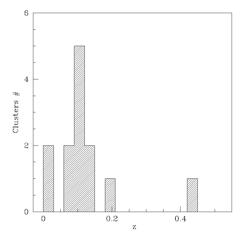
Figure 1: Redshift distribution of clusters in the field of view with a redshift identification.

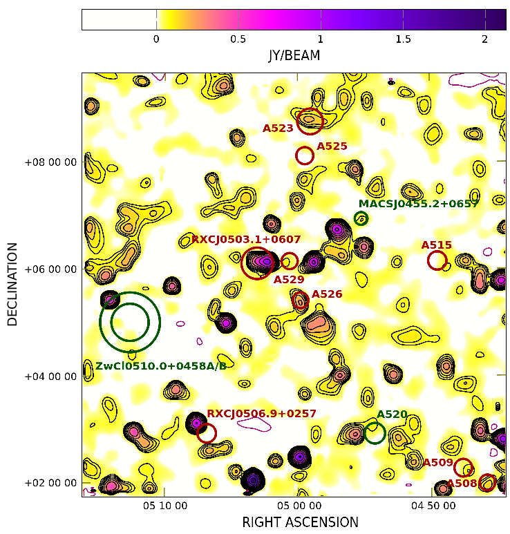
Figure 2: SRT image in colours and contours in the frequency range 1.3-1.8 GHz. The contours are -3$\sigma$, 3$\sigma$ ($\sigma=20$ mJy/beam) and the remaining scale by a factor $\sqrt{2}$. Negative contours are represented in magenta, while positive contours are in black. The angular resolution of the images is 13.9${}^{\prime}\times$12.4^′ and BPA=-58.5^∘ at the center of the observing band. The circles and labels identify the position of the galaxy clusters in the field of view with known redshift. The size of the circles is proportional to $R_{200}$ of the corresponding clusters (see Table 4), large circles are close-by clusters while small circles are distance clusters. For systems with an upper limit for $R_{200}$, we used the value of the upper limit. We highlight in red clusters with redshift between 0.08 and 0.15, in green clusters with redshift outside this range.

2.1 Abell 520

This galaxy cluster is a dynamically young system, undergoing a strong merger event in the NE-SW direction (Govoni et al., 2004). In radio, it is famous for hosting an extended synchrotron source with a largest linear size of 1.4 Mpc, originally classified as a radio halo (Giovannini et al., 1999; Govoni et al., 2001), with the south-west edge of the radio emission coincident with a bow shock, as found by Markevitch et al. (2005). A recent re-analysis of the radio emission in the cluster revealed that the radio halo has a flux density at 1.4 GHz of $S_{\rm 1.4\,GHz}=(16.7\pm 0.6)$ mJy (Vacca et al., 2014). The peculiar morphology and properties of the source do not reflect the typical properties of radio halos and raise new questions about its nature, as noted already by Govoni et al. (2001). By using optical observations from the Telescopio Nazionale Galileo and the Isaac Newton Telescope facilities, Girardi et al. (2008) found evidence that the cluster formation is taking place at the crossing of three filaments: one in the north-east/south-west direction, one in the east-west direction, and one almost aligned with the line of sight.

2.2 Abell 523

According to Chow-Martínez et al. (2014), A523 is an isolated galaxy cluster. It consists of an irregular south/south-west sub-cluster strongly interacting with a more compact sub-cluster on the north/north-east direction (Girardi et al., 2016). The system has been discovered to host large-scale diffuse radio emission (Giovannini et al., 2011) in the form of a radio halo located at the center of the cluster with a flux $S_{\rm 1.4\,GHz}=(59\pm 5)\,$mJy and a largest linear angular size of 12^′. According to a re-analysis of the radio data by Girardi et al. (2016), this source has a flux density at 1.4 GHz of $S_{\rm 1.4\,GHz}=(72\pm 3)$ mJy, a largest linear size of 1.3 Mpc and it is characterized by a polarized signal. Polarization is uncommon among radio halos. It has been detected in only other two cases, A2255 (Govoni et al., 2005) and MACS J0717+3745 (Bonafede et al., 2009), and indicates an intra-cluster magnetic field fluctuating on scales as large as hundreds of kpc. Compared to the other radio halos, this system is under-luminous in X-rays with respect to radio, opening new questions on the formation of radio halos and their link with merger events.

Table 2: Clusters in the field without redshift information.

Cluster	RA (J2000)	Dec (J2000)
	h:m:s	∘:′:′′
ZwCl 0440.1+0514	04:42:45.5	+05:19:37
ZwCl 0440.3+0547	04:42:58.2	+05:52:36
ZwCl 0440.9+0407	04:43:32.3	+04:12:34
ZwCl 0441.7+0423	04:44:20.6	+04:28:30
ZwCl 0444.7+0828	04:47:25.2	+08:33:18
ZwCl 0445.1+0223	04:47:42.4	+02:28:16
ZwCl 0445.6+0539	04:48:16.1	+05:44:14
ZwCl 0446.2+0235	04:48:48.6	+02:40:12
ZwCl 0446.6+0150	04:49:11.8	+01:55:10
ZwCl 0448.2+0919	04:50:56.2	+09:24:03
ZwCl 0448.5+0551	04:51:10.3	+05:56:02
ZwCl 0451.3+0159	04:53:54.0	+02:03:51
ZwCl 0452.1+0627	04:54:47.0	+06:31:47
HSTJ 045648+03529	04:56:48.3	+03:52:57
ZwCl 0454.3+0534	04:56:58.0	+05:38:38
ZwCl 0455.3+0155	04:57:53.9	+01:59:34
ZwCl 0455.2+0746	04:57:54.5	+07:50:34
ZwCl 0457.0+0511	04:59:39.6	+05:15:26
ZwCl 0458.2+0137	05:00:47.6	+01:41:22
ZwCl 0458.5+0102	05:01:04.9	+01:06:20
ZwCl 0458.5+0536	05:01:10.1	+05:40:20
ZwCl 0459.2+0212	05:01:48.2	+02:16:17
ZwCl 0459.6+0606	05:02:16.7	+06:10:15
ZwCl 0459.8+0943	05:02:32.8	+09:47:14
ZwCl 0502.0+0350	05:04:38.1	+03:54:05
ZwCl 0502.1+0201	05:04:42.0	+02:05:05
ZwCl 0503.1+0751	05:05:48.7	+07:55:01
ZwCl 0504.9+0417	05:07:32.6	+04:20:53
ZwCl 0505.1+0655	05:07:47.6	+06:58:52
ZwCl 0508.8+0241	05:11:24.8	+02:44:36

Col 1: Cluster name; Col 2 & 3: cluster coordinates.

3 Radio Observations

In order to look for the presence of diffuse emission from low density environments connecting galaxy clusters, we observed with the SRT a region of the sky hosting nine clusters with redshift z$\approx$0.1: A523, A525, RXC J0503.1+0607, A529, A515, A526, RXC J0506.9+0257, A509, and A508, see Table 1. The radio observations presented in this paper were done in the context of the SRT Multi-frequency Observations of Galaxy Clusters program (SMOG, PI. Matteo Murgia, see Govoni et al., 2017; Loi et al., 2017, for a description of the project). We observed an area of $8^{\circ}\times 8^{\circ}$ centred at right ascension (RA) 05h:00m:00.0s and declination (Dec) +05^∘:48^′:00.0^′′, for a total exposure time of about 18 hours and three smaller fields of view centred respectively on the galaxy clusters A520, A526, and A523 over a region of $3^{\circ}\times 3^{\circ}$ of about 1.5 hour each. The observations were taken with the L- and P-band dual-frequency coaxial receiver for primary-focus operations (Valente et al., 2010). We used the L-band component only covering the frequency range 1.3-1.8 GHz. The data stream was recorded with the SArdinia Roach2-based Digital Architecture for Radio Astronomy (SARDARA Melis et al., 2018) back-end. The configuration used had 1500 MHz of bandwidth and 16384 channels $\sim$90 kHz each, full-Stokes parameters, and sampling at 10 spectra per second. We opted for the on-the-fly (OTF) mapping strategy scanning the sky alternatively along the RA and Dec direction with a telescope scanning speed of 6 ^′/s and an angular separation of 3 ^′ between scans, this choice guarantees a proper sampling of the SRT beam whose full width at half maximum (FWHM) is 13.9 ${}^{\prime}\times$12.4 ^′ at 1550 MHz, the central frequency of these observations. Since the sampling time is 100 ms, the individual samples are separated in the sky by 36 ^′′ along the scanning direction. A detailed summary of the SRT observations is given in Table 3.

The calibration and the imaging of the data were performed with the proprietary Single-dish Spectral-polarimetry Software (SCUBE, Murgia et al., 2016). We used 3C 147 as band-pass and flux density calibrator and the flux density scale of Perley & Butler (2013) was assumed. We flagged about 23% of the data because of radio frequency interference (RFI). After calibration, a baseline was fitted to the data in order to subtract any emission not related to the target (due e.g, to our Galaxy). The subtraction of the baseline has been performed as follows. First, we convolved the NVSS image of this region to the resolution of the SRT. We used this image to identify empty regions in the SRT image. The linear fit of the emission of these regions was then subtracted from the data. The baseline-subtracted data were then projected in a regular three-dimensional (RA - Dec - observing frequency) grid with a spatial resolution of 3 ^′/pixel in order to guarantee a beam FWHM sampling of four pixels. These steps were performed in each frequency channel. The resulting frequency cube was stacked and de-stripped by mixing the Stationary Wavelet Transform (SWT) coefficients (see Murgia et al., 2016, for details). This image was then used to produce a new mask and the procedure was repeated. This procedure was performed for each dataset separately and the images produced for each dataset were averaged.

Finally, we applied a hard threshold denoising algorithm on scales below two pixels (1 pixel=3 ^′) as the signal amplitude is expected to be negligible with respect to the noise amplitude on these angular scales. The denoised image obtained by the combination of all the SRT data is shown in Fig. 2 in colours and contours. The noise level 1$\sigma$ of the radio image is 20 mJy/beam, comparable with the confusion noise for this frequency band at the SRT resolution. The zero-level of the image is $\sim$25% of the noise level. A detailed description of the calibration and imaging procedures of the SRT data are given in Murgia et al. (2016) and Govoni et al. (2017).

The circles and labels in Fig. 2 indicate the position in the field of the clusters with a redshift identification. This figure reveals that most of the nine clusters with redshift $\approx$ 0.1 are all located along a line crossing the field of view from north to south and connecting the galaxy clusters A523 and A508, passing through A525, RXC J0503.1+0607, A529, A526, and A509, while RXC J0506.9+0257 and A515 are respectively slightly south-east and slightly west of the filament. A520 has a redshift higher than the average redshift of this group. A possible explanation is that A520 appears to belong to this region of the sky only because of projection effects. Alternatively, the filament could be partially located in the plane of the sky and partially oriented along the line of sight in the direction of A520. This is supported by the findings of Girardi et al. (2008) which suggest the hypothesis that A520 could be connected with the filament at z$\approx$0.1 examined in this work. However, as shown in Table 1, the redshift of A520 implies a distance along the line of sight of about 410 Mpc, therefore the hypothesis of a connection is still controversial.

3.1 SRT beam and calibration scale

We cross-checked the calibration procedures by comparing the SRT flux scale with the NVSS flux scale. To perform the comparison, we produced SRT images in the same frequency range as the NVSS images, we tailored from the whole SRT bandwidth (1.3-1.8 GHz) two smaller sub-bands centred at the same frequencies and with the same width of the NVSS observations (1364.9 - 1414.9 MHz and 1435.1 - 1485.1 MHz) and then binned them in one image.

As a first step, we measured the beam of the SRT images by fitting the emission of the brightest isolated point source in the field with the software SCUBE (Murgia et al., 2016). This compact source is a quasar with redshift $z=2.384$ (Xu & Han, 2014) and is located at RA J2000 04h:59m:53.94s and Dec J2000 02^∘:29^′:39.72^′′ (see Fig. 3, left panel). By fitting the peak emission with a circular 2-d Gaussian with four free parameters (peak, $x$ and $y$ coordinates of the centre, and FWHM), we obtained for the SRT beam a FWHM of $\theta=(820\pm 1)\,^{\prime\prime}$.

We then compared the SRT and NVSS flux scales by fitting the peak brightness of the brightest non-variable isolated point-source. The source is located at RA J2000 05h:05m:24.21s and Dec J2000 04^∘:59^′:48.44^′′ (see Fig. 3, right panel). During the fitting procedure the beam FWHM was kept fixed to the value derived above. The position of the peak as measured by the SRT and by the NVSS agrees within 15^′′. The peak in the two images are in agreement within about 10%, with a value respectively of ($0.96\pm 0.03$) Jy/beam and ($0.86\pm 0.03$) Jy/beam. Note that the source used for the fit is not the brightest source in the field but one among the brightest isolated sources. Indeed, we prefer to discard non-isolated sources because of possible blending of sources. Moreover, we note that the flux scale of the NVSS and of SRT observations are based respectively on the scales by Baars et al. (1977) and Perley & Butler (2013), and they agree within 1%.

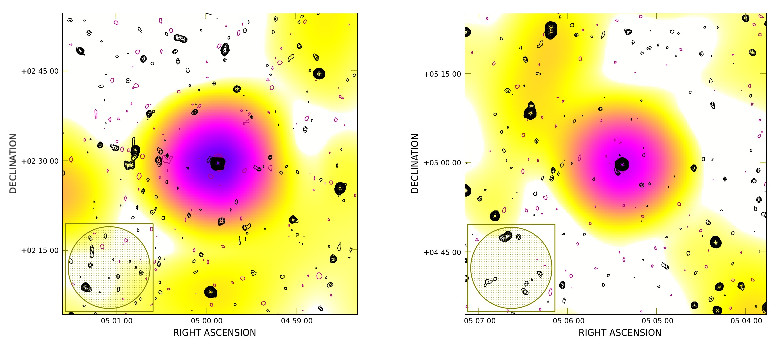
Figure 3: Sources used for the beam measurement (left panel) and for the comparison of the NVSS and SRT flux density scales (right panel). The SRT image in the same frequency range as the NVSS is shown in colours, while the NVSS emission is shown in contours. The contour levels are -1.35, 1.35 mJy/beam (with a beam of 45^′′) and increase by a factor $\sqrt{2}$, positive contours shown in black and negative contours shown in magenta. The beam in the bottom left corner represents the SRT spatial resolution of 13.66^′ as found in § 3.1. The colorbar is the same as Fig. 2.

4 Combination of single-dish and interferometric data

In this section, we present the combination of our single-dish data with mosaic interferometric observations taken from the NVSS, following the approach described by Loi et al. (2017). Single-dish observations can recover a maximum angular scale corresponding to the angular size of the scanned region but they miss high spatial resolution. Interferometers can reach high spatial resolutions but are limited by the maximum angular scale corresponding to their minimum baseline. In the case of a full-synthesis Very Large Array (VLA) observation this translates to $\sim$16^′ for the most compact configuration at L-band. For snapshot observations as the NRAO VLA Sky Survey (NVSS, Condon et al., 1998) this number should be divided by two but we consider the full angular size since the NVSS image we used has been obtained with a mosaic. By combining the SRT and NVSS data, we retain the ability to observe large-scale structures up to 8^∘ and, at the same time, the resolution of the VLA in D configuration at 1.4 GHz, i.e. 45^′′. The combination has been performed in the Fourier domain with the SCUBE software package (Murgia et al., 2016). The SRT has a size of 64 m, while the VLA in its most compact configuration has a minimum baseline of 35 m, this means that there is a common range of spacing and consequently of wave-numbers $k$ in the Fourier space. We combined the NVSS image with the SRT image obtained in the same frequency range and select in this image the same region of the sky as the NVSS image, so that they should contain the same radio power.

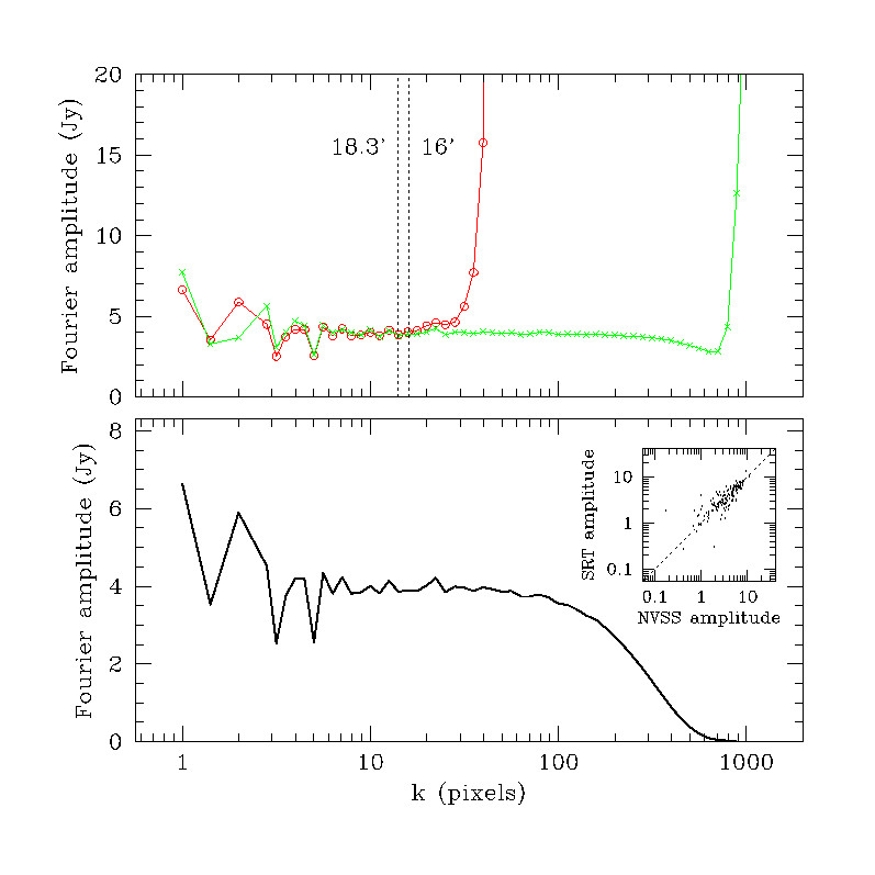
Figure 4: Top panel: Power spectrum of the SRT data (red) and power spectrum of the NVSS data (green). The dashed vertical black lines identify the overlapping region used to adjust the flux density scales. Bottom panel: Tapered combined power spectrum. In the inset the comparison between the amplitude of the SRT and of the NVSS data in the region of overlapping (18.3^′-16^′) in the Fourier space is shown.

In order to combine the two images we required that the two power spectra have the same power spectral density in the inner portion of the overlapping region in Fourier-space, corresponding to angular scales between 16^′ and 18.3^′. This requirement translates into a scaling factor of the SRT power spectrum normalization of $\approx$1.003. In § 3.1, by comparing the flux of a single source in the two images, we found that the two flux density scales agree within 10%. In this section we make a more robust statistical comparison, by using all the sources available in the field. This agreement confirms the accuracy of the SRT flux density scale calibration.

The two power spectra were then merged with a weighted sum: the single-dish data-weights were set to zero for angular scales smaller than 16^′, to 1 for angular scales larger than 18.3^′, and with a weight that linearly varies from 0 to 1 in between. Vice-versa for the interferometric data-weights. The final power spectrum was tapered with the interferometric beam and the data were back-transformed to obtain the combined image. The interferometric and single-dish power spectra are shown in the top panel of Fig. 4, after the beam deconvolution (they have been divided in Fourier space by the Fourier transform of the corresponding beam). The merged power spectrum is shown in the bottom panel of Fig. 4: in the inset the SRT amplitude versus the NVSS amplitude is shown for measurements corresponding to angular scales in the overlapping region. The average of the amplitude of the points in the inset corresponds to the value shown in the large panels. The combined image has a beam of 45^′′ and a noise 0.45 mJy/beam, dominated by the NVSS noise. To better highlight the presence of diffuse large-scale sources, we convolved to a beam of $3.5^{\prime}\times 3.5^{\prime}$. The resulting combined image is shown in Fig. 6 (grey colours, top panels).

Table 3: Data

Date	Receiver	Target	FOV	OFT scan axis	Calibrators	Time on source
14Jul2016	L-band	A520-A526-A523	$8^{\circ}\times 8^{\circ}$	1$\times$(RA$+$Dec)	3C84,3C147, 3C138	10 h
23Jul2016	L-band	A520-A526-A523	$8^{\circ}\times 8^{\circ}$	1$\times$(RA$+$Dec)	3C286,3C147, 3C138	9 h
22Jul2016	L-band	A520	$3^{\circ}\times 3^{\circ}$	1$\times$(RA$+$Dec)	3C84,3C147, 3C138	1 h 20 min
22Jul2016	L-band	A523	$3^{\circ}\times 3^{\circ}$	1$\times$(RA$+$Dec)	3C84,3C147, 3C138	1 h 40 min
22Jul2016	L-band	A526	$3^{\circ}\times 3^{\circ}$	1$\times$(RA$+$Dec)	3C84,3C147, 3C138	1 h 20 min

4.1 Point source subtraction

To investigate the presence of large-scale diffuse structures associated with the galaxy clusters reported in Table 1 and with the low-density environments connecting them, we performed a subtraction of the point sources with the SCUBE software package (Murgia et al., 2016) in the combined image at $45^{\prime\prime}$ resolution.

The subtraction is done as follows:

• the strongest point source in the image is identified and fitted with a non-zero baseline 2-d elliptical Gaussian;

• the model is then subtracted from the image;

• the two steps above are repeated until an user-defined threshold is reached.

To take into account the possibility that each source is embedded into large-scale diffuse emission, we model the source with a 2-d elliptical Gaussian sitting on a plane. Overall, the free parameters of the fit are nine: the $x,y$ coordinates in the sky of the centre of the Gaussian, the FWHM along the two axis, the position angle, the amplitude, and the three components of the direction normal to the plane. Only in the case of sources weaker than a user-defined-threshold (in this case 10$\sigma$) is the FWHM is forced to assume the value of the beam size. This algorithm has been tested in the context of Fatigoni (2017).

As outputs, the task produces a residual image. We repeated the procedure two times. At first, we used a threshold of about 7$\sigma$=3 mJy/beam, where $\sigma$=0.45 mJy/beam is the noise of the image. As a second step, we again run the algorithm on the residual image, with a lower threshold of 4$\sigma$=1.8 mJy/beam. This conservative threshold has been chosen to avoid over-subtraction. In total, 3872 sources have been subtracted. In Fig. 6 (top right and bottom left panels), the resulting residual image is shown in blue contours. In Appendix A we use a sub-sample of the radio galaxies in the field to cross check the flux scale after the combination of single-dish and interferometric data.

5 X-ray emission

The X-ray properties of the majority of the clusters in the sample are unknown. Information for only a few of the clusters in Table 1 can be found in the literature. The X-ray luminosity of A523, RXC J0506.9+0257, and RXC J0503.1+0607 are reported in the catalogue by Böhringer et al. (2000), while A520 and MACS J0455.2+0657 can be found in Mahdavi et al. (2007) and Mann & Ebeling (2012), respectively. To our knowledge, no information is available for the remaining clusters.

By applying the approach proposed by Finoguenov et al. (2007), we derived the flux $S_{\rm X}$ in the 0.5-2 keV energy band and the luminosity $L_{\rm X,0.1-2.4\,keV}$ within an extraction area of radius $R_{200}$ for the clusters in Table 1, by using data from the ROSAT All-Sky Survey (RASS, Voges et al., 1999). The fluxes of the clusters have been corrected for the aperture and for the Point Spread Function and the luminosities have been corrected for the dimming (for details about the procedure please refer to Finoguenov et al., 2007). The values of flux and luminosity of these clusters are reported in Table 4. For the sources with significance of the count rate below 1$\sigma$, the values we provide for all the properties are 2$\sigma$ upper limits.

Table 4: X-ray fluxes of galaxy clusters

Cluster	z	$n_{\rm H}$	$R_{200}$	$M_{200}$	$S_{\rm X}$	$D_{\rm L}$	$L_{\rm X,0.1-2.4\,keV}$
		$10^{20}$ cm-2	∘	$10^{14}M_{\odot}$	$10^{-12}$erg s-1 cm-2	Mpc	$10^{43}$erg s-1
A523	0.104	10.6	0.192	2.91	1.6 $\pm$ 0.3	499	7.3 $\pm$ 1.6
A525	0.1127	9.98	0.128	1.08	0.3 $\pm$ 0.1	543	1.6 $\pm$ 0.8
MACSJ0455.2+0657	0.425	8.41	0.096	12.87	1.3 $\pm$ 0.2	2416	116.1 $\pm$ 21.6
ZwCl0510.0+0458A	0.027	12.0	< 0.28	< 0.19	< 0.4	123	< 0.1
ZwCl0510.0+0458B	0.015	12.0	< 0.448	< 0.14	< 0.7	68	< 0.1
RXCJ0503.1+0607	0.088	8.61	0.235	3.39	2.9 $\pm$ 0.4	418	9.0 $\pm$ 1.4
A529	0.1066	8.25	< 0.121	< 0.79	< 0.2	512	< 0.9
A515	0.1061	8.21	0.137	1.12	0.3 $\pm$ 0.2	509	1.6 $\pm$ 0.8
A526	0.1068	7.81	0.117	0.72	0.2 $\pm$ 0.1	513	0.8 $\pm$ 0.6
RXCJ0506.9+0257	0.1475	8.57	0.14	2.91	0.8 $\pm$ 0.2	727	7.7 $\pm$ 2.1
A520	0.199	5.66	0.155	8.64	2.6 $\pm$ 0.4	1011	45.0 $\pm$ 6.1
A509	0.0836	8.88	< 0.133	< 0.53	< 0.2	395	< 0.5
A508	0.1481	9.85	0.118	1.75	0.4 $\pm$ 0.2	730	3.5 $\pm$ 1.5

Col 1: Cluster name; Col 2: redshift; Col 3: cluster Hydrogen column density; Col 4: $R_{200}$ of the system; Col 5: X-ray flux in the 0.5-2 keV energy band within $R_{200}$; Col 6: Mass of the galaxy cluster within $R_{200}$; Col 7: Luminosity distance; Col 8: X-ray luminosity in the 0.1-2.4 keV energy band within $R_{200}$.

6 millimetre and sub-millimetre emission

To investigate the properties of the cosmic web in this region of the sky, we superimposed the SRT contours on the Planck image, see Fig. 6 (colours, bottom left panel). The Compton parameter map (hereafter $Y$-map) has been obtained by using the data from the full mission and by applying the Modified Internal Linear Combination Algorithm (MILCA Hurier et al., 2013) method. As described in the work by Planck Collaboration et al. (2016a), this method removes the signal of the Cosmic Microwave Background taking into account its spectral properties.

Most of the clusters in Table 1 show a counterpart in the Planck image. However, in the catalogue by Planck Collaboration et al. (2016b) only an association for A520 and one for A539 (RA 05:16:37.3, Dec +06:26:16, z=0.0284) within 4^′ are present. The strongest signal is detected in the direction of A523 and A520, where it extends well beyond the cluster outskirts. A signal appears to be present also in the direction of A525, A529, RXC J0503.1+0607, MACS J0455.2+0657, RXC J0506.9+0257, A515, A508, A509, and A539 but, unfortunately, the galaxy cluster A539 is at the edge of the SRT field of view. On the contrary, for A526 and ZwCl 0510.0+0458 A/B there is no evidence of a signal above the noise level.

7 Results

The SRT contours reveal a field rich of radio sources. This region of the sky is populated by several galaxy clusters starting from the north with the complex A523-A525 down to the south with the complex A508-A509. A large fraction of them are approximately at the same redshift ($\approx$0.1, see Fig. 1), and possibly form a filament of the cosmic web sitting in the plane of the sky. This hypothesis is supported by the fact that some of them have been observed to be undergoing accretion processes as confirmed by the diffuse large-scale synchrotron emission observed at their centre. This is the case of A523 and A520, even if it is not clear whether A520 belongs to the filament because of its large distance along the line of sight. In the CDM cosmology, clusters of galaxies with a mass exceeding $10^{14}$ $M_{\odot}$ should have a 80% probability of being connected to a neighbouring cluster by a filamentary joint of dark and gas matter, in case they are less than 15 Mpc $h^{-1}$ apart (Colberg et al., 2005). Based on the X-ray data (Table 4) we can estimate that at least eight of the clusters (A523, A525, MACS J0455.2+0657, RXC J0503.1+0607, A515, RXC J0506.9+0257, A520, and A508) in the field have a mass $M_{\rm 200}\geq 10^{14}M_{\odot}$. Therefore, several of these objects might be connected by filaments difficult to observe through the X-ray/SZ effect but possibly detectable in the radio window. In Fig. 5, we show the distribution of 3-d distances between all the pairs of clusters with known redshift in the field. Since an absolute error in the redshift estimate of 0.003 (3%) translates in an error in the 3-d distance of about 13 Mpc$h^{-1}$, we looked for pairs with 3-d distance in the range 0–30 Mpc$h^{-1}$. We found five pairs within this range of 3-d distance (A526 and RXC J0503.1+0607, A526 and A529, A509 and RXCJ0503.1+0607, A509 and A529 and A509 and A526), suggesting that this field is likely to host filaments of dark and gas matter connecting galaxy clusters.

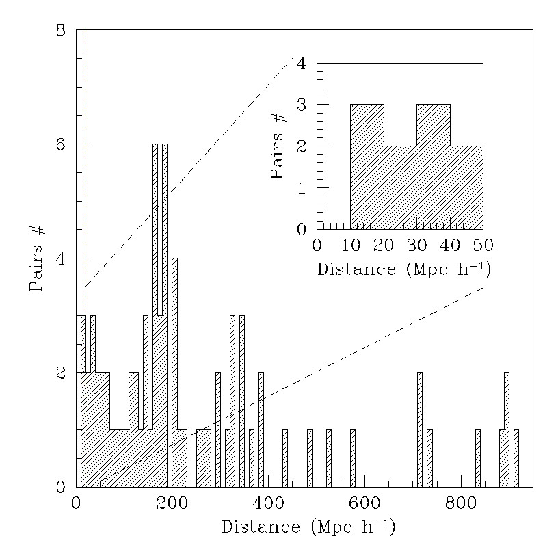
Figure 5: Distribution of 3-d distances between all the pairs of clusters with known redshift in the field. The dashed vertical blue line marks a 3-d distance of 15 Mpc$h^{-1}$. In the inset a zoom of the region between 0 and 50 Mpc$h^{-1}$ is shown.

To identify possible diffuse radio emission in the field and better understand its nature, we subtracted the point sources and compared the residual radio emission with the signal observed at other wavelengths. In the following we present the results and describe the properties of the diffuse radio sources we found.

7.1 Diffuse emission

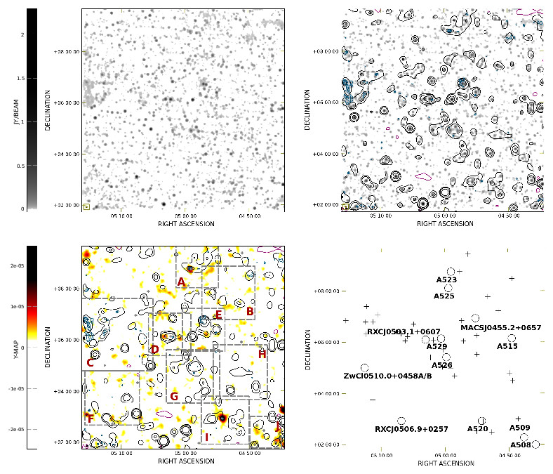
Figure 6: Top left panel: SRT+NVSS image in colours (FWHM 3.5^′). Top right panel: contours of the SRT image (-60 mJy/beam, 60 mJy/beam, 150 mJy/beam, 500 mJy/beam, negative in magenta and positive in black; resolution 13.9 ${}^{\prime}\times$12.4 ^′) and of the SRT+NVSS image after compact sources subtraction (starting at 3$\sigma$ and increasing by a factor $\sqrt{2}$, in blue; $\sigma$=2.5 mJy/beam, resolution 3.5${}^{\prime}\times$3.5^′) overlaid on the SRT+NVSS image in colours (FWHM 3.5^′). Bottom left panel: SRT and SRT+NVSS after point-source subtraction in contours overlaid on the Planck Y-map (see text) in colours. The contours from SRT and from the residual SRT+NVSS image are the same as in the top right panel. The resolution of the Planck Y-map is 10^′. Dots indicate the position of clusters with redshift identification (see Table 1), while crosses indicate clusters without redshift identification (see Table 2). Bottom right panel: Location of clusters with known redshift (circles and labels) and of the sources discussed in this paper (crosses), see Table 5.

In this section we inspect the SRT, the SRT+NVSS and the residual SRT+NVSS after compact source subtraction images at 1.4 GHz (see Fig. 6, top right panel) and compare them with X-ray ROSAT data in the 0.1–2.4 keV from the RASS and the SZ Compton parameter from millimetre/sub-millimetre observations obtained with the Planck satellite.

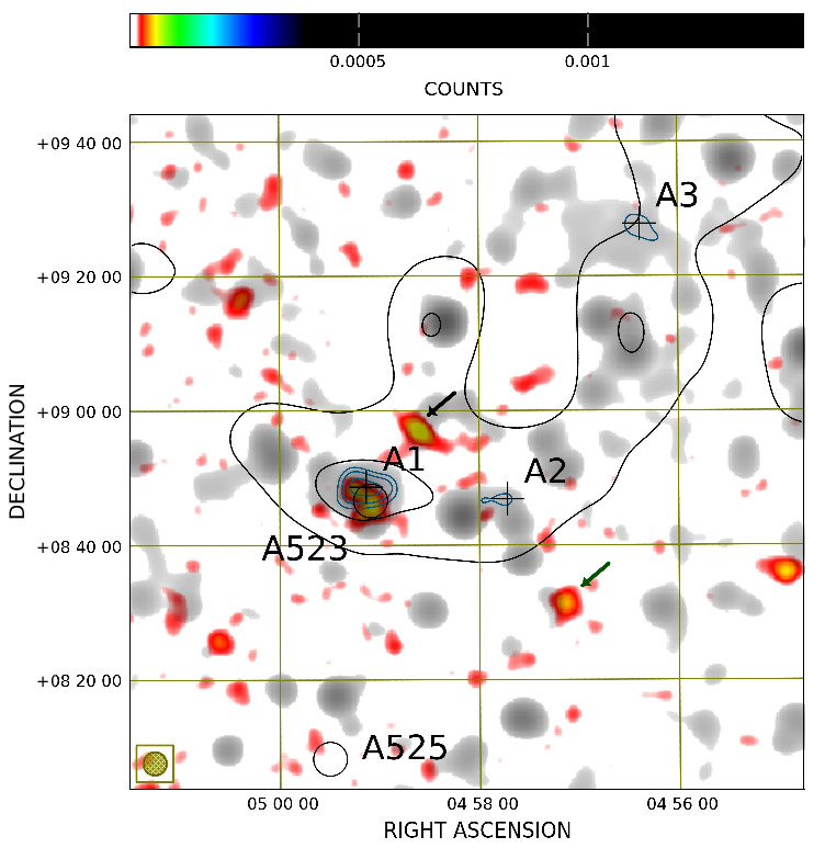
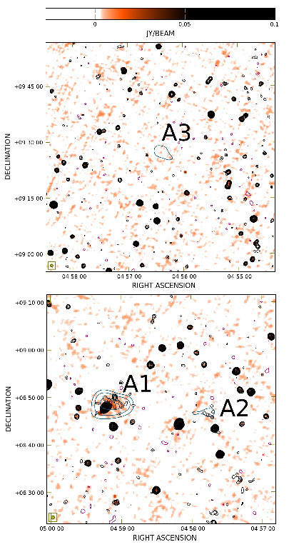
Figure 7: Region A. Left panel: SRT contours (-60 mJy/beam, 60 mJy/beam, 150 mJy/beam, 500 mJy/beam, negative in magenta and positive in black; resolution 13.9 ${}^{\prime}\times$12.4 ^′) and SRT+NVSS after compact sources subtraction contours (in blue, starting from 3$\sigma$ and the remaining increasing by a factor $\sqrt{2}$; $\sigma$=2.5 mJy/beam, resolution 3.5${}^{\prime}\times$3.5^′) overlaid on X-ray emission from the RASS in red colours and radio emission from the SRT+NVSS (resolution $3.5^{\prime}$) in gray colours. Right panels: NVSS contours -3$\sigma$ (magenta, $\sigma$=0.45 mJy/beam), 3$\sigma$, and increasing by a factor $\sqrt{2}$ (black) overlaid on the TGSS in colours. The black and green arrows mark regions where a strong X-ray emission is detected, as described in the text.

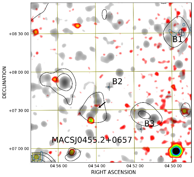
Figure 8: Region B. Left panel: SRT contours (-60 mJy/beam, 60 mJy/beam, 150 mJy/beam, 500 mJy/beam, negative in magenta and positive in black; resolution 13.9 ${}^{\prime}\times$12.4 ^′) and SRT+NVSS after compact sources subtraction contours (in blue, starting from 3$\sigma$ and the remaining increasing by a factor $\sqrt{2}$; $\sigma$=2.5 mJy/beam, resolution 3.5${}^{\prime}\times$3.5^′) overlaid on X-ray emission from the RASS in red colours and radio emission from the SRT+NVSS (resolution $3.5^{\prime}$) in gray colours. Right panels: NVSS contours -3$\sigma$ (magenta, $\sigma$=0.45 mJy/beam), 3$\sigma$, and increasing by a factor $\sqrt{2}$ (black) overlaid on the TGSS in colours. The black arrow marks the region shown in the zoom of Fig. 9. The colorbars are the same as in Fig. 7.

Figure 9: Zoom of the central portion of Region B (see arrow in Fig. 8). The image shows the NVSS contours (-1.35 mJy/beam, 1.35 mJy/beam, and the remaining scaled by a factor $\sqrt{2}$, negative in magenta and positive in black) overlaid on the TGSS colours. The colorbar is the same as in the right panels of Fig. 7.

After the subtraction of the compact sources, 35 patches of diffuse synchrotron emission survive, whose locations are shown in Fig. 6 along with the location of the clusters with redshift identification (bottom right panel). The sources are mainly located along the group of clusters with redshift z$\approx$0.1 (A523, A525, RXC J0503.1+0607, A529, A515, A526, RXC J0506.9+0257, A508, and A509), and in the region around A539 (middle left of the image). We identified eight regions of interest where these 35 candidate sources are located (gray boxes in the bottom left panel of Fig. 6). Due to the large size of the field of view, to better visualize these diffuse radio sources, we present a zoom of each region in figures from Fig. 7 to Fig. 17, labelled respectively with capital letters from A to J (see Fig. 6). In each Figure, on the left panel, we overlay the SRT and the SRT+NVSS contours after the point-source subtraction on the X-ray and SRT+NVSS images in colours. On the right panel(s), we show the NVSS contours overlaid on the TIFR GMRT Sky Survey Alternative Data Release (TGSS ADR, Intema et al., 2017) in colours. We indicate the position of the clusters with redshift identifications with circles and labels and mark all the spots of diffuse emission with a cross and the letter corresponding to the region of interest plus progressive numbers. These sources are those visible in the residual image after a 3$\sigma$ cut in radio brightness ($\sigma=2.5$ mJy/beam). For these sources, we give an estimate of the flux ($S_{\rm residual}$) and the largest linear size (LLS) in Table 5. In order to evaluate the integrated flux and the size of these sources, we blanked the convolved residual image at its 2$\sigma$ level. A summary of the radio and X-ray properties of these sources is given in Table 5 and Table 6 respectively. Sources at the edge of the image have not been considered because they could be artefacts of the imaging or point-source subtraction process. The only exception is the patch of diffuse emission close-by the galaxy cluster A539. In the following we report a description of the emission observed in each region.

7.1.1 Region A

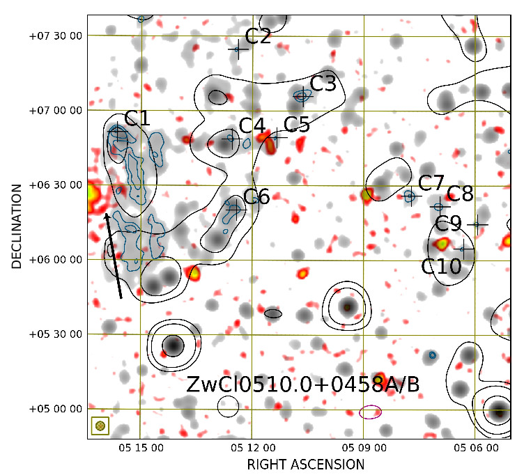
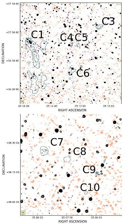
Figure 10: Region C. Left panel: SRT contours (-60 mJy/beam, 60 mJy/beam, 150 mJy/beam, 500 mJy/beam, negative in magenta and positive in black; resolution 13.9 ${}^{\prime}\times$12.4 ^′) and SRT+NVSS after compact sources subtraction contours (in blue, starting from 3$\sigma$ and the remaining increasing by a factor $\sqrt{2}$; $\sigma$=2.5 mJy/beam, resolution 3.5${}^{\prime}\times$3.5^′) overlaid on X-ray emission from the RASS in red colours and radio emission from the SRT+NVSS (resolution $3.5^{\prime}$) in gray colours. Right panels: NVSS contours -3$\sigma$ (magenta, $\sigma$=0.45 mJy/beam), 3$\sigma$, and increasing by a factor $\sqrt{2}$ (black) overlaid on the TGSS in colours. The black arrow marks the position of A539. The colorbars are the same as in Fig. 7.

Moving from north to south of the full field of view, the first object is A523 (Fig. 7), which hosts a powerful radio halo (Giovannini et al., 2011) also visible in the NVSS. This system is known to be over-luminous in radio with respect to the X-rays. The SRT data indicate a large-scale emission with an elongation to the west of A523. After subtracting the point sources in the combined SRT+NVSS image, a residual diffuse emission emerges at the position of A523 (source A1) and another 12^′ (source A2), west of A1. A few patches of diffuse emission can be seen also on the north-west (source A3), where hints of radio emission are already visible in the combined SRT+NVSS image. At the location of sources A2 and A3 no point source emission is detected in the NVSS image. X-ray emission is clearly visible toward A523 and to the north-west (see black arrow in the image), while only hints of emission are present at the location of A2 and A3. South-west of A2, an X-ray signal is detected (green arrow), whose diffuse nature is uncertain. By inspecting the high resolution NVSS and TGSS images corresponding to the X-ray signal, we find hints of diffuse emission. In the SRT+NVSS image after point source subtraction, a diffuse patch at 2$\sigma$ of significance is detected at the same spatial location.

In the residual image, we measure a flux of the radio halo in A523 of (44$\pm$5) mJy and a largest linear size (LLS) of about 1.2 Mpc (10^′). As a comparison, Giovannini et al. (2011) give a flux $S_{\rm 1.4\,GHz}=(59\pm 5)\,$mJy, while Girardi et al. (2016) report $S_{\rm 1.4\,GHz}=(72.3\pm 0.6)\,$mJy. The integrated flux measured in this work is slightly weaker than that estimated by Giovannini et al. (2011). This difference can be explained by the different procedures of point-sources subtraction. The corresponding radio power at 1.4 GHz is 1.33$\times$10²⁴W/Hz. The shape and the size of the radio halo in the galaxy cluster A523 from our images are very similar to those previously derived from interferometric observations only. The source appears quite roundish with a slight elongation in the direction perpendicular to the merger axis (SSW-NNE), as derived by X-ray and optical data (Girardi et al., 2016).

7.1.2 Region B

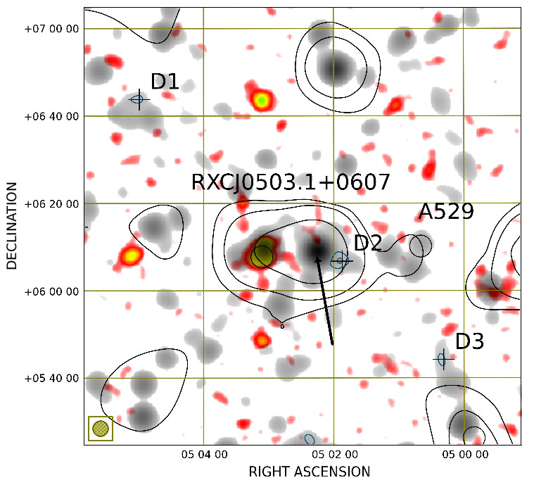
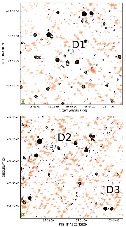
Figure 11: Region D. Left panel: SRT contours (-60 mJy/beam, 60 mJy/beam, 150 mJy/beam, 500 mJy/beam, negative in magenta and positive in black; resolution 13.9 ${}^{\prime}\times$12.4 ^′) and SRT+NVSS after compact sources subtraction contours (in blue, starting from 3$\sigma$ and the remaining increasing by a factor $\sqrt{2}$; $\sigma$=2.5 mJy/beam, resolution 3.5${}^{\prime}\times$3.5^′) overlaid on X-ray emission from the RASS in red colours and radio emission from the SRT+NVSS (resolution $3.5^{\prime}$) in gray colours. Right panels: NVSS contours -3$\sigma$ (magenta, $\sigma$=0.45 mJy/beam), 3$\sigma$, and increasing by a factor $\sqrt{2}$ (black) overlaid on the TGSS in colours. The black arrow marks the position of the quasar PKS 0459+060. The colorbars are the same as in Fig. 7.

In Fig. 8, we show the region to the south-west of A523. In the top right corner of the image, an excess of radio emission is detected by the SRT (source B1). Some point sources can be identified in the outskirts of it but not embedded in the emission, excluding the possibility that this source is a blending of point-like sources. Two other diffuse patches of emission can be identified in the field (source B2 and B3), not clearly associated with point-like sources but rather located at positions where an excess in radio emission is observed in the combined SRT+NVSS image (refer to Macario et al., 2014, for a similar case). At the location of Source B2 a hint of diffuse emission is observed also in the NVSS and TGSS images.

According to the literature, no galaxy cluster is present in the field shown in Fig. 8. However, high resolution NVSS and TGSS data (Fig. 9) show that the emission detected by the SRT at the centre of the panel, south-east of B2, is a blending of compact radio sources that might be part of a galaxy cluster. In a region of radius 20^′ centred on the radio galaxy indicated by the arrow in Fig. 8, only the source 2MASX J04534530+0719303 located at RA 04h53m45.3s and Dec +07d19m31s has a spectroscopic redshift measurement (z=0.104, Rines et al., 2003). These galaxies could be part of a galaxy cluster or a group of galaxies at the same redshift of the filament.

7.1.3 Region C

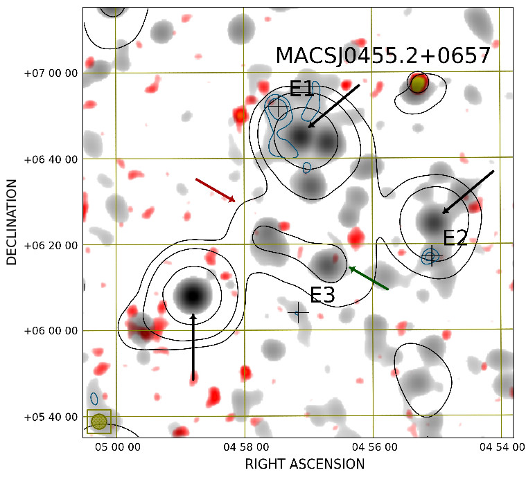
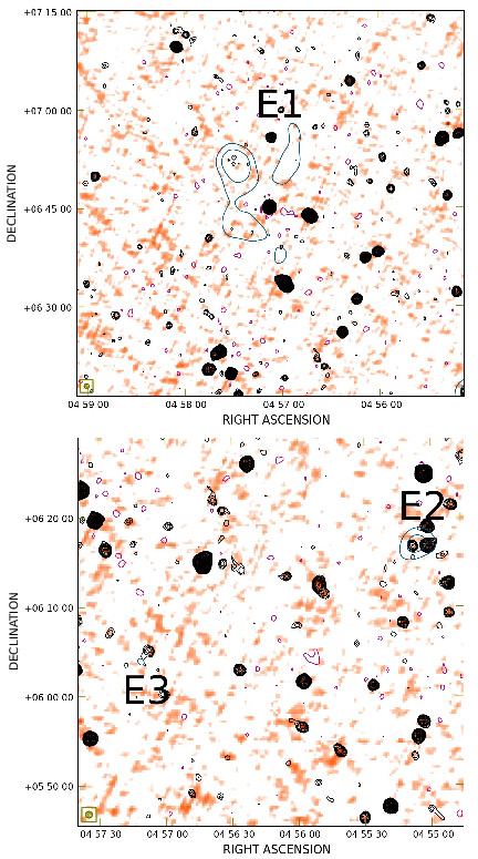
Figure 12: Region E. Left panel: SRT contours (-60 mJy/beam, 60 mJy/beam, 150 mJy/beam, 500 mJy/beam, negative in magenta and positive in black; resolution 13.9 ${}^{\prime}\times$12.4 ^′) and SRT+NVSS after compact sources subtraction contours (in blue, starting from 3$\sigma$ and the remaining increasing by a factor $\sqrt{2}$; $\sigma$=2.5 mJy/beam, resolution 3.5${}^{\prime}\times$3.5^′) overlaid on X-ray emission from the RASS in red colours and radio emission from the SRT+NVSS (resolution $3.5^{\prime}$) in gray colours. Right panels: NVSS contours -3$\sigma$ (magenta, $\sigma$=0.45 mJy/beam), 3$\sigma$, and increasing by a factor $\sqrt{2}$ (black) overlaid on the TGSS in colours. The black arrows mark the position of 4C +06.21, PKS 0456+060, and LQAC 073+006 001, and the red arrow the faint large-scale emission SRT emission in between these three bright compact sources. The green arrow marks the location where signal is clearly visible in the SZ and X-ray images while in the SRT+NVSS after compact sources subtraction is is detected only with a 2$\sigma$ significance. The colorbars are the same as in Fig. 7.

East of the filament, another region of interest can be identified (see Fig. 10) on the west of the galaxy cluster A539, whose position is indicated by the arrow in the same Figure. The cluster appears to be an emitter in the X-ray and millimetre/sub-millimetre domain but, unfortunately, it is outside the field of view of our SRT observations and only the regions to its west has been mapped. In the SRT image, we see a large arm extending from the cluster westward, still visible in the residual image as a large diffuse structure. This structure can not be explained as the blending of radio galaxies in the field, so it is likely related to a large-scale diffuse source. After the subtraction of point sources, ten patches (Sources from C1 to C10) remain. Apart from C1, C6 and C9 could be at least partially the leftovers of the point-like source subtraction process, the remaining sources seem to be large-scale diffuse synchrotron sources. Among these, the largest and more interesting is C1. Hints of diffuse large-scale emission at the same spatial location are present in the SRT+NVSS and in the X-ray image. A slight excess of large-scale radio emission can be identified as well at higher resolution in the NVSS. However, since it is located at the edge of the image, more observations are required to confirm it and investigate its nature.

7.1.4 Region D

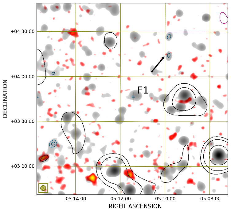
Figure 13: Region F. Left panel: SRT contours (-60 mJy/beam, 60 mJy/beam, 150 mJy/beam, 500 mJy/beam, negative in magenta and positive in black; resolution 13.9 ${}^{\prime}\times$12.4 ^′) and SRT+NVSS after compact sources subtraction contours (in blue, starting from 3$\sigma$ and the remaining increasing by a factor $\sqrt{2}$; $\sigma$=2.5 mJy/beam, resolution 3.5${}^{\prime}\times$3.5^′) overlaid on X-ray emission from the RASS in red colours and radio emission from the SRT+NVSS (resolution $3.5^{\prime}$) in gray colours. Right panel: NVSS contours -3$\sigma$ (magenta, $\sigma$=0.45 mJy/beam), 3$\sigma$, and increasing by a factor $\sqrt{2}$ (black) overlaid on the TGSS in colours. The black arrow marks the position of the candidate giant radio galaxy we found (see § B). The colorbars are the same as in Fig. 7.

The complex RXC J0503.1+0607 - A529 is located at the centre of the panel shown in Fig. 11 and the galaxy cluster ZwCl 0459.6+0606 sits between them (see Table 2). In the bottom right corner of the image, the galaxy cluster A526 is also partially visible. In the X-rays, only RXC J0503.1+0607 shows a signal above the noise level. In radio, both RXC J0503.1+0607 and A529 can be seen: RXC J0503.1+0607 is a strong emitter, while A529 is characterized by a faint signal. The peak observed in the SRT image between the two clusters is approximately at the same angular location as ZwCl 0459.6+0606 (see arrow in Fig. 11) and is due to the quasar PKS 0459+060 (RA 05h02m15.4s, Dec +06d09m07s, z=1.106). The superposition of the SRT and the SRT+NVSS images, reveals the presence of several point sources in the field, as well as hints of large-scale emission in between the two clusters. This indication is confirmed by the residual image, where patches of large-scale diffuse emission are present (D1, D2, and D3). Source D1 in the top left corner is located in a region where the SRT+NVSS image reveals a large-scale patch of radio emission. Source D2 does not show a connection with point-like sources in the field and appear located at the periphery of ZwCl 0459.6+0606. Indications of the presence of a large-scale signal at locations of D1 and D2 can be seen in the NVSS image. A puzzling patch of diffuse emission is observed to the south-west (source D3), in the outskirts of A526, without a clear association with any point sources but rather corresponding to hints of diffuse emission in the SRT+NVSS images.

7.1.5 Region E

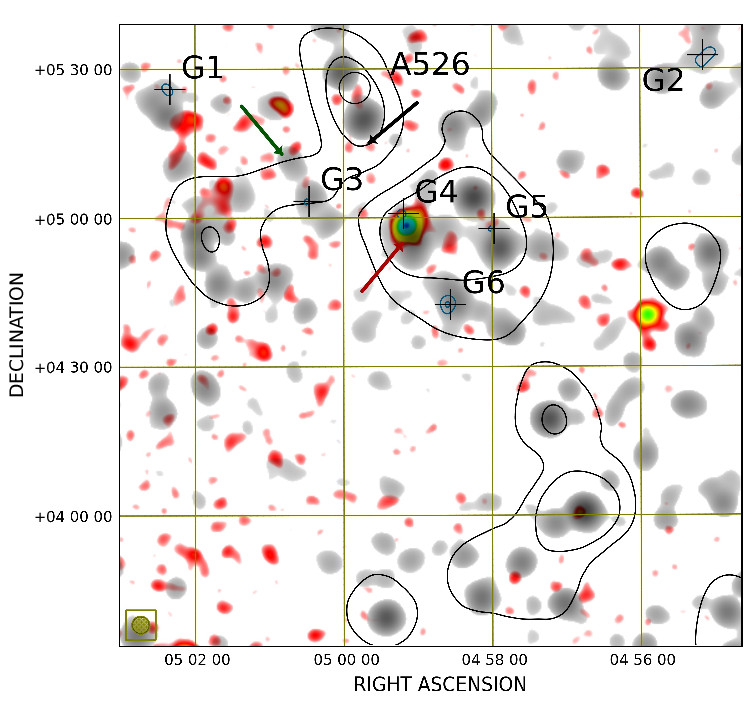
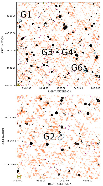
Figure 14: Region G. Left panel: SRT contours (-60 mJy/beam, 60 mJy/beam, 150 mJy/beam, 500 mJy/beam, negative in magenta and positive in black; resolution 13.9 ${}^{\prime}\times$12.4 ^′) and SRT+NVSS after compact sources subtraction contours (in blue, starting from 3$\sigma$ and the remaining increasing by a factor $\sqrt{2}$; $\sigma$=2.5 mJy/beam, resolution 3.5${}^{\prime}\times$3.5^′) overlaid on X-ray emission from the RASS in red colours and radio emission from the SRT+NVSS (resolution $3.5^{\prime}$) in gray colours. Right panels: NVSS contours -3$\sigma$ (magenta, $\sigma$=0.45 mJy/beam), 3$\sigma$, and increasing by a factor $\sqrt{2}$ (black) overlaid on the TGSS in colours. The black and red arrow mark respectively the locations of the galaxy cluster ZwCl 0457.0+0511 and of the compact source PMN J0459+0455, while the green arrow a bridge of radio emission detected by SRT. The colorbars are the same as in Fig. 7.

In Fig. 12, another interesting complex can be identified 2^∘ south of A523, south-east of the galaxy cluster MACS J0455.2+0657. In this region, MACS J0455.2+0657 is the only galaxy cluster with a spectroscopic redshift measurement ($z=0.425$). In the field of view of Fig. 12, the SRT image reveals three bright peaks (see black arrows in Fig. 12) and a faint large-scale emission in between them (red arrow). At higher resolution, several point sources can be identified. Three of them have the same spatial location as the three peaks detected by the SRT: 4C +06.21 (RA 04h57m07.7099s, Dec +06d45m07.260s, z=0.405, Drinkwater et al., 1997), PKS 0456+060 (RA 04h58m48.782s, Dec +06^∘08^′04.26^′′, z= 1.08, Veron-Cetty & Veron, 1996), and LQAC 073+006 001 (RA 04h55m03.1s, Dec +06^∘24^′54^′′, no redshift identification). After point source subtraction, three interesting large-scale patches emerge. One off the bright radio source 4C +06.21 (source E1), one some 10^′ south of LQAC 073+006 001 (source E2), and one south of the central radio emission (source E3), where no emission appears in the SRT image above the noise level. The source E1 does not appear to be a blending of point-like sources as shown by the superposition with higher resolution data in Fig. 12 and hints of large-scale diffuse emission are already present in the NVSS image. E1 is characterized by an average brightness of $\approx$ 0.13 $\mu$Jy/arcsec², its integrated flux density is (109 $\pm$ 10) mJy, and its largest angular size is 25^′. If we assume that this emission is at the same redshift as the radio source 4C +06.21 (z=0.405), its LLS is 8.7 Mpc and its radio power at 1.4 GHz is 6.8$\times$10²⁵ W/Hz. However, if we assume that this source is located at the average redshift of the filament ($z\approx 0.1$), its LLS is about 3 Mpc and its radio power at 1.4 GHz is 3.0$\times$10²⁴ W/Hz. No strong X-ray emission is present in the field except that seen to the north-east of the radio source E1. Source E3 is located at position where the combined NVSS indicates the presence of an excess of large-scale diffuse emission, while the source E2 could be the residual of point-like emission. At the centre of the panel, at coordinates RA 04h56m25.24s, Dec +06^∘13^′29^′′ (see green arrow), a 2$\sigma$-level signal is observed in the residual radio image. Since it is below the 3$\sigma$ significance threshold, we did not consider it in our analysis. However, at the same spatial location, a faint X-ray emission and a SZ signal (see Fig. 6) are present, suggesting that these emissions could be real and not a statistical fluctuation.

7.1.6 Region F

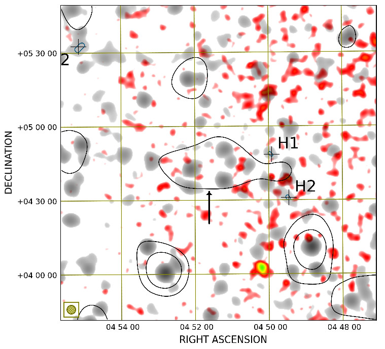
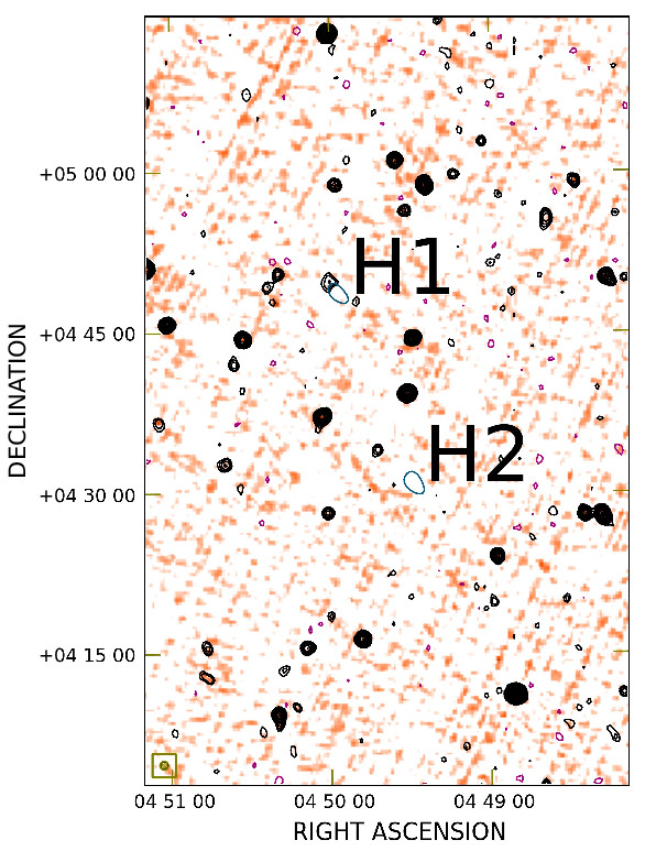
Figure 15: Region H. Left panel: SRT contours (-60 mJy/beam, 60 mJy/beam, 150 mJy/beam, 500 mJy/beam, negative in magenta and positive in black; resolution 13.9 ${}^{\prime}\times$12.4 ^′) and SRT+NVSS after compact sources subtraction contours (in blue, starting from 3$\sigma$ and the remaining increasing by a factor $\sqrt{2}$; $\sigma$=2.5 mJy/beam, resolution 3.5${}^{\prime}\times$3.5^′) overlaid on X-ray emission from the RASS in red colours and radio emission from the SRT+NVSS (resolution $3.5^{\prime}$) in gray colours. Right panel: NVSS contours -3$\sigma$ (magenta, $\sigma$=0.45 mJy/beam), 3$\sigma$, and increasing by a factor $\sqrt{2}$ (black) overlaid on the TGSS in colours. The black arrow marks a blending of point-like sources. The colorbars are the same as in Fig. 7.

In the region shown in Fig. 13 no galaxy cluster is identified in ṯhe literature. The field is rich in point-like radio sources as shown by the SRT+NVSS image. The SRT+NVSS image after point source subtraction shows five patches of diffuse emission. The two on the left side are not considered here, since they are at the edge of the image and might be artefacts. The two spots in the top right region reveal an extended radio galaxy (see arrow in the image) that we classify as a candidate new giant radio galaxy and discuss in Appendix B. Our interest here is the source F1 located at the centre of the image. This source is located close-by a point-like source, spatially coincident with a fainter large-scale region visible also in the NVSS image.

7.1.7 Region G

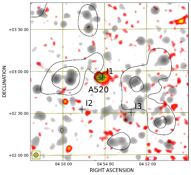
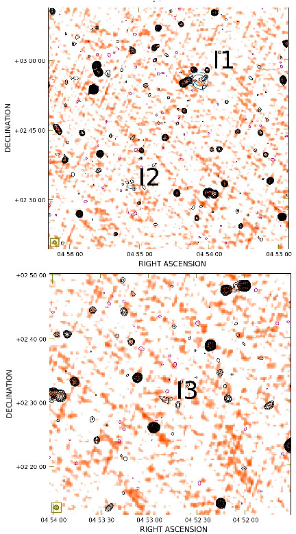
Figure 16: Region I. Left panel: SRT contours (-60 mJy/beam, 60 mJy/beam, 150 mJy/beam, 500 mJy/beam, negative in magenta and positive in black; resolution 13.9 ${}^{\prime}\times$12.4 ^′) and SRT+NVSS after compact sources subtraction contours (in blue, starting from 3$\sigma$ and the remaining increasing by a factor $\sqrt{2}$; $\sigma$=2.5 mJy/beam, resolution 3.5${}^{\prime}\times$3.5^′) overlaid on X-ray emission from the RASS in red colours and radio emission from the SRT+NVSS (resolution $3.5^{\prime}$) in gray colours. Right panels: NVSS contours -3$\sigma$ (magenta, $\sigma$=0.45 mJy/beam), 3$\sigma$, and increasing by a factor $\sqrt{2}$ (black) overlaid on the TGSS in colours. The colorbars are the same as in Fig. 7.

The galaxy cluster A526 is shown in the top of Fig. 14. The cluster is visible in radio and X-rays, but shows no counterpart at millimetre/sub-millimetre wavelengths. To the south-west, large-scale emission is detected with the SRT. No galaxy clusters have been identified in this region apart from the galaxy cluster ZwCl 0457.0+0511 (see black arrow in the image), south-west of A526 at an angular offset of about 10^′. Two strong X-ray sources are seen: one south of A526, approximately coincident with the radio source PMN J0459+0455 (RA 04h59m04.7s, Dec +04d55m59s, see red arrow) and the other in the west with no obvious radio counterpart. After subtracting the point source emission, several patches of diffuse emission emerge. Source G1 and G2, respectively in the top left and right corners, have the same spatial location of an excess in the NVSS image. Another patch of residual radio emission is present in the north-east of the image (source G3), close-by to a point source surrounded by a fainter large-scale signal and where the SRT image shows a bridge of radio emission (see green arrow) connecting A526 with an over-density of radio galaxies south-east of A526. At the centre of the panel, three patches of diffuse emission are present corresponding to the large-scale central SRT radio emission: sources G4, G5, G6. Sources G4 and G5 appear to be diffuse sources, while source G6 could be a residual of the point source located below.

7.1.8 Region H

This region (Fig. 15) is full of point-like sources as shown by the SRT+NVSS image. In the SRT image a central patch likely due to the blending of point-like sources is present (see arrow in the image). Above and below this emission, two patches of residual radio signal (sources H1 and H2) are identified that do not appear to be directly linked to point-like sources. In particular, at the location of H1, an indication of diffuse emission is detected also in the NVSS image.

7.1.9 Region I

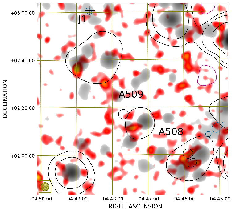
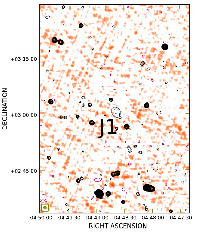
Figure 17: Region J. Left panel: SRT contours (-60 mJy/beam, 60 mJy/beam, 150 mJy/beam, 500 mJy/beam, negative in magenta and positive in black; resolution 13.9 ${}^{\prime}\times$12.4 ^′) and SRT+NVSS after compact sources subtraction contours (in blue, starting from 3$\sigma$ and the remaining increasing by a factor $\sqrt{2}$; $\sigma$=2.5 mJy/beam, resolution 3.5${}^{\prime}\times$3.5^′) overlaid on X-ray emission from the RASS in red colours and radio emission from the SRT+NVSS (resolution $3.5^{\prime}$) in gray colours. Right panel: NVSS contours -3$\sigma$ (magenta, $\sigma$=0.45 mJy/beam), 3$\sigma$, and increasing by a factor $\sqrt{2}$ (black) overlaid on the TGSS in colours. The colorbars are the same as in Fig. 7.

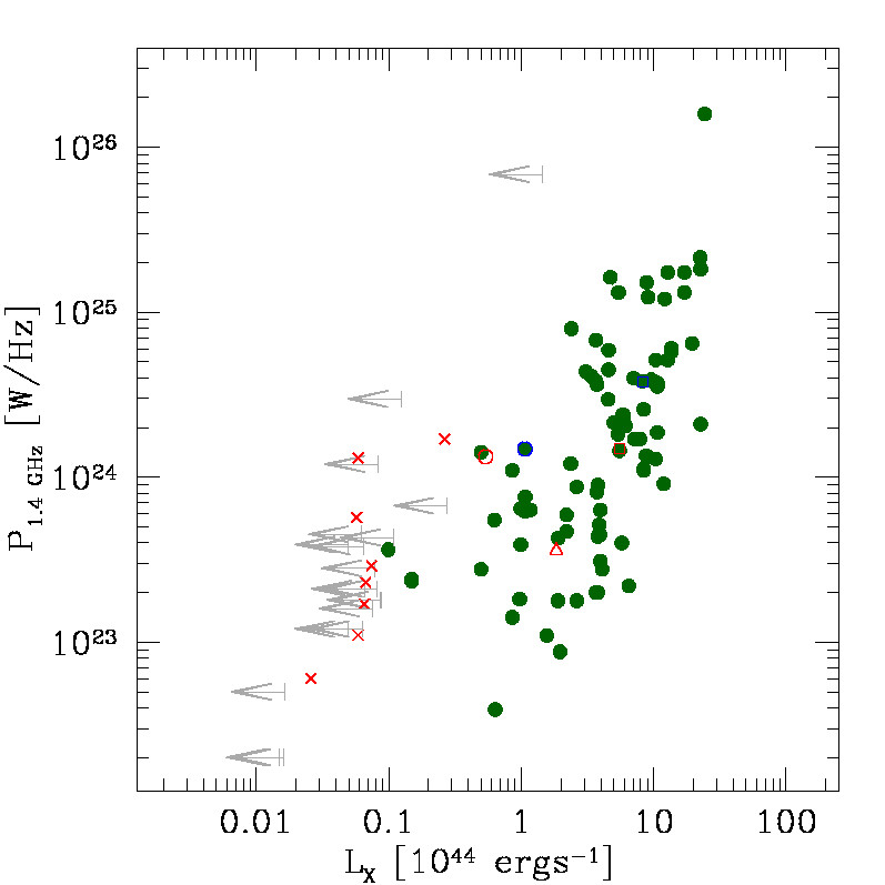
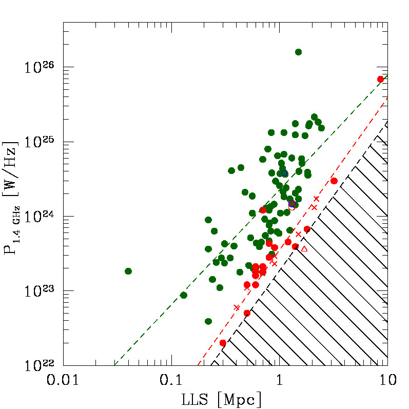
Figure 18: Left panel: Radio power at 1.4 GHz $P_{\rm 1.4\,GHz}$ versus X-ray luminosity in the energy band 0.1-2.4 keV $L_{\rm X,0.1-2.4\,keV}$. Right panel: Radio power $P_{\rm 1.4\,GHz}$ versus LLS both at 1.4 GHz. Green dots and blue open symbols are from Feretti et al. (2012). Red symbols are measurements from this work: open symbols identify A523 (circle), A520 (square), G4 (triangle), while crosses identify the remaining sources with an X-ray identification. Grey arrows are upper limits from this work. The shaded area in the right panel indicates the region of the ($P_{\rm 1.4\,GHz}$, LLS) plane that cannot be accessed considering the 2$\sigma$ ($\sigma$=2.5 mJy/beam) sensitivity of the SRT+NVSS image after point source subtraction. Dashed lines represent a linear fit in logarithmic scale of Eq. 1 for cluster sources (green) and for the new sources (red).

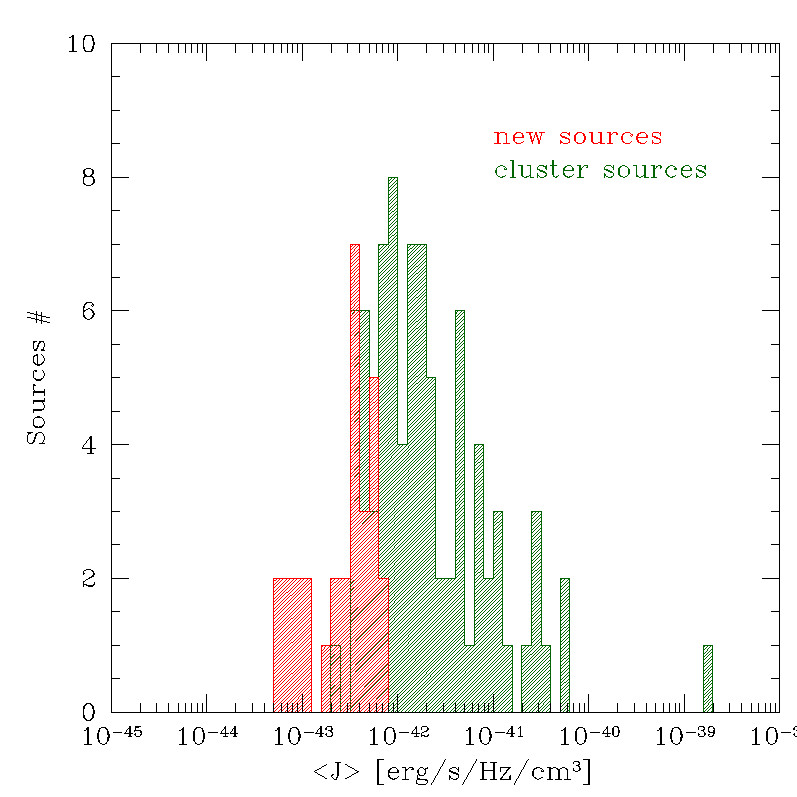
Figure 19: Histogram in logarithmic scale of the mean emissivity of the new sources presented in this paper (red) compared to the cluster diffuse radio sources from Feretti et al. (2012) (green).

At the centre of Fig. 16 the galaxy cluster A520 is present, located in the south of the full field of view. Strong X-ray emission is spatially coincident with this cluster, that appears to be very bright at millimetre/sub-millimetre wavelengths (see Fig. 6). Hints of diffuse emission are present in the NVSS in the direction of A520 (where indeed a radio halo is present), east, south and south-west of the cluster. After the point source subtraction in the SRT+NVSS image, patches of diffuse large-scale emission remain at these locations and the radio halo in A520 (source I1) is now clearly visible. In the residual image blanked at the 2$\sigma$ level, we measure an integrated flux of (12 $\pm$ 3) mJy and a LLS of about 1 Mpc for this radio halo. The corresponding radio power at 1.4 GHz is 1.48$\times$10²⁴ W/Hz. As a comparison, the values reported in the literature are (16.7$\pm$0.6) mJy and 1.05 Mpc (Govoni et al., 2001; Vacca et al., 2014) which are very consistent with ours. South of A520, the sources I2 and I3 can be observed. They do not show a clear link with radio galaxies in the field, on the contrary they are located where hints of diffuse radio emission are present in the NVSS image, so they could be real large-scale diffuse synchrotron sources. The present observations of the radio halo in the galaxy cluster A520 confirm what was suggested by the data at higher resolution. The source is quite complex and with a strong elongation in the NE-SW direction. The peak of the emission is located in the SW at the same location as the shock front (Markevitch et al., 2005; Govoni et al., 2004), where a sharp drop in radio surface brightness is detected. A faint tail of radio emission is left behind in the cool region. As already suggested by Govoni et al. (2001) and Vacca et al. (2014), this peculiar source could actually be a peripheral source seen in projection.

7.1.10 Region J

The complex A508-A509 sits in the south-east corner of the full field of view and is shown in Fig. 17. The two clusters are also visible in X-rays and at millimetre/sub-millimetre wavelengths but they are quite faint. Patches of diffuse emission not coincident with point-like sources survive in the residual image. Source J1 is located where an excess of radio emission is observed in the NVSS image. The other patches are located at the edge of the image and are therefore hard to discriminate if they are real or artefacts, even though the SRT+NVSS image clearly shows a patch of diffuse emission before compact-source subtraction.

Table 5: Diffuse large-scale emission properties of sources detected above 3$\sigma$

Source	RA (J2000)	Dec (J2000)	z	$S_{\rm residual}$	$P_{\rm 1.4\,GHz}$	LLS	Class	Alternative name
	h:m:s	d:m:s		mJy	$10^{23}$W/Hz	Mpc
A1	04:59:08.81	+08d48:52	0.104	45 $\pm$ 5	13.3	1.3		Radio halo A523
A2	04:57:43.81	+08d47:03	0.104	10 $\pm$ 3	2.9	0.9
A3	04:56:23.85	+09d27:59	0.104	44 $\pm$ 7	13.1	2.1
B1	04:49:29.06	+08d30:16	0.104	100$\pm$ 10	29.7	3.2
B2	04:53:19.21	+07d48:11	0.100	4 $\pm$ 2	1.2	0.5
B3	04:51:39.15	+07d15:01	0.100	5 $\pm$ 2	1.2	0.6
C1	05:15:39.81	+06d51:47	0.029	554$\pm$ 27	11.6	2.6	*
C2	05:12:24.80	+07d25:01	0.029	8 $\pm$ 3	0.2	0.3
C3	05:10:39.64	+07d06:07	0.029	28 $\pm$ 5	0.6	0.4
C4	05:12:34.29	+06d49:01	0.029	23 $\pm$ 5	0.5	0.5
C5	05:11:21.76	+06d49:35	0.029	10 $\pm$ 3	0.2	0.3
C6	05:12:26.81	+06d20:31	0.029	55 $\pm$ 7	1.2	0.8	*
C7	05:07:44.04	+06d26:13	0.100	16 $\pm$ 4	4.3	0.8
C8	05:06:57.73	+06d21:59	0.100	21 $\pm$ 5	5.7	1.5
C9	05:05:57.34	+06d14:45	0.100	4 $\pm$ 2	1.1	0.5	*
C10	05:06:19.45	+06d04:59	0.100	7 $\pm$ 3	2.1	0.7
D1	05:05:00.00	+06d44:00	0.100	6 $\pm$ 2	1.8	0.7
D2	05:01:52.93	+06d06:57	0.100	17 $\pm$ 4	4.5	1.2
D3	05:00:19.57	+05d44:24	0.100	14 $\pm$ 4	3.9	1.4
E1	04:57:26.67	+06d52:01	0.405	109$\pm$ 10	684.7	8.6
E2	04:55:05.24	+06d17:21	0.100	12 $\pm$ 3	3.4	0.8	*
E3	04:57:10.28	+06d04:15	0.100	4 $\pm$ 2	1.1	0.5
F1	05:11:24.89	+03d46:42	0.100	7 $\pm$ 3	12.0	0.7
G1	05:02:21.28	+05d26:12	0.100	6 $\pm$ 2	1.6	0.6
G2	04:55:03.01	+05d33:20	0.100	14 $\pm$ 4	3.8	0.9
G3	05:00:28.93	+05d03:38	0.100	6 $\pm$ 3	1.7	0.7
G4	04:59:12.63	+05d01:05	0.100	13 $\pm$ 4	3.6	1.7
G5	04:57:59.36	+04d58:01	0.100	8 $\pm$ 3	2.3	0.9
G6	04:58:34.65	+04d42:47	0.100	15 $\pm$ 4	4.0	1.2	*
H1	04:49:56.16	+04d48:46	0.100	7 $\pm$ 3	1.8	0.6
H2	04:49:28.39	+04d31:12	0.100	10 $\pm$ 3	2.8	0.8
I1	04:54:06.90	+02d55:46	0.199	12 $\pm$ 3	14.9	1.3		Radio halo A520
I2	04:55:06.23	+02d33:02	0.199	5 $\pm$ 2	6.7	1.8
I3	04:52:45.95	+02d30:33	0.199	14 $\pm$ 4	17.0	2.2
J1	04:48:37.81	+03d00:55	0.100	8 $\pm$ 3	2.1	0.6

Col 1: Source label; Col 2 & 3: source coordinates; Col 4: redshift; Col 5: Flux density at 1.4 GHz of the residual diffuse emission from the SRT+NVSS combined image after the point source-subtraction; Col 6: Radio power at 1.4 GHz of the diffuse emission; Col 7: Largest linear size of the diffuse emission; Col 8: An asterisk indicates that the source could be a leftover of compact sources after the subtraction process or an artefact; Col 9: Alternative name of the source.

8 Discussion

After subtracting the point-source emission, we identified 35 patches of diffuse synchrotron emission in the residual SRT+NVSS image. Two of them are the radio halos in the galaxy clusters A520 and A523, and five are probably artefacts or the leftover of point-like sources after the point-source subtraction process. The remaining 28 are potentially new real large-scale diffuse synchrotron sources, possibly associated with the large-scale structure of the cosmic web. The bottom right panel of Fig. 6 shows that most of the new sources presented in this paper lie along the filament connecting the clusters from A523-A525 in the north to A508-A509 in the south, with an over-density at the centre of the field of view, at the location of RXC J0503.1+0607, A529 and A526. In the following, we restrict our analysis to the properties of the 28 new detections and the two radio halos already known. We excluded sources that could be artefacts or a remnant of compact sources after the subtraction procedure. To better investigate their properties, we measured their radio powers and sizes and their X-ray luminosities, summarized in Table 5 and in Table 6 respectively. The X-ray fluxes have been estimated by following the procedure described in § 5. Only eleven sources have a significance of the X-ray count rate above 1$\sigma$. These sources are A1 (diffuse emission in A523), A2, A3, C3, C8, E3, G3, G4, G5, I1 (diffuse emission in A520), and I3.

Some of the sources presented here are potentially interesting and complex systems. For example, source A2 is a faint large-scale source 10^′ west of the radio halo in A523 (source A1). It has a radio flux at 1.4 GHz $S_{\rm residual}=(9\pm 3)$ mJy ($P_{\rm 1.4\,GHz}=2.8\times 10^{23}$ W/Hz), a LLS of 1.3 Mpc, and an X-ray luminosity $L_{\rm X0.1-2.4\,keV}=(0.7\pm 0.6)\times 10^{44}$ erg/s. In the south-west of A2, another diffuse patch of synchrotron emission is detected at 2$\sigma$ significance and at the same spatial location of an X-ray signal (see § 7.1.1). These three sources could form an arc-shaped filament of diffuse synchrotron emission. If A2 and the source south-west of it are interpreted to be radio halos, Source A1 - Source A2 and this third source could represent the first case of a triple radio halo, which would be particularly interesting because of its association with an under-luminous X-ray system. To, date only one other multiple system is known, namely the double radio halo discovered by Murgia et al. (2010) in the galaxy cluster couple A399-A401. In that case the two clusters are about 2.4 Mpc apart, while in this case the distance between these sources is about 1.4 Mpc if all of them are at the same redshift of Source A1 (z=0.104). A follow up at the X-ray and optical frequencies is needed to understand if at this location other galaxy clusters are present and shed light on the nature of these sources.

An even more mysterious source is the emission we label E1. This source appears to be exactly along the long filament connecting A523-A525 in the north to A509-A508 in the south-west, and in the same direction of the radio galaxy 4C +06.21, embedded in the diffuse emission and sitting at redshift z=0.405. There is no indication in the literature of a galaxy cluster at the same location in the sky and the closest galaxy clusters to the source are MACS J0455.2+065 ($\approx 25^{\prime}$) and A529 (at about $50^{\prime}$). Therefore, Source E1 could be either associated with the filament or a diffuse large-scale structure in the background, as suggested by the redshift of the closest radio source. Source E1 is the most luminous and most extended source in the sample, with a flux at 1.4 GHz $S_{\rm residual}=(109\pm 10)$ mJy ($P_{\rm 1.4\,GHz}=6.8\times 10^{25}$ W/Hz), a LLS of 8.7 Mpc, assuming it is at the same redshift of 4C +06.21 (z=0.405). On the other hand, if we assume that the source is at the same redshift of the filament (z$\approx$0.1), we derive a radio power $P_{\rm 1.4\,GHz}=3.0\times 10^{24}$ W/Hz and an LLS=3 Mpc, still among the brightest and largest sources of the sample. Nevertheless, the source is very faint in the X-ray, for which we derive a luminosity $L_{\rm X,0.1-2.4\,keV}<14.5\times 10^{44}$ erg/s (2$\sigma$) if a redshift z=0.405 is taken. A firm classification is not possible without further information about the system over a wide range of frequencies, from the X-ray to optical and radio bands.

Overall, the nature of the above sources remains unclear. To investigate if they are similar to diffuse cluster sources (i.e. radio halos and relics, e.g., Feretti et al., 2012) or rather they represent a different population, we compare the radio power, radio size and X-ray luminosity of these new sources with those of known diffuse cluster sources. Hereafter, we adopt for known cluster sources the values given by Feretti et al. (2012) without applying any correction for the cosmology. In Fig. 18, we show in the left panel the radio power at 1.4 GHz $P_{\rm 1.4\,GHz}$ versus the X-ray luminosity $L_{\rm X,0.1-2.4\,keV}$ in the energy band 0.1–2.4 keV and in the right panel the radio power at 1.4 GHz $P_{\rm 1.4\,GHz}$ versus the largest linear scale LLS at 1.4 GHz, for cluster sources (radio halos and radio relics) from Feretti et al. (2012) and for the new sources presented in this work. For the diffuse emission in A523 and A520 (Sources A1 and I1), we plot both the values we derive and the values found in the literature in order to have a basis for comparison. Our values are slightly different than the values available in the literature, as discussed in § 7.1, but still follow the correlation between radio and X-ray properties for known diffuse radio sources. Among the eleven sources in our catalogue with a significance of the X-ray count rate above 1$\sigma$, two are the radio halos in A520 and A523, one (G4) follows the correlation observed for radio halos and relics, and the remaining eight show a X-ray luminosity between 10 and 100 times lower than expected from their radio power given the correlation observed for cluster sources, with an average X-ray luminosity of $L_{\rm X,0.1-2.4\,keV}$=0.77$\times 10^{44}$ erg/s. They populate a new region of the ($L_{\rm X,0.1-2.4\,keV}$, $P_{\rm 1.4\,GHz}$) plane that was previously unsampled. The remaining sources are very faint. They show a radio power comparable to that of radio halos, but with fainter X-ray emission ($\lesssim 10^{43}$ erg/s) and larger size. Their nature is quite mysterious, since they are located in a region of the sky where no galaxy cluster has been identified in the literature.

The radio power versus largest linear size diagram (right panel of Fig. 18) is interesting, as extended diffuse radio sources in clusters are known to follow the correlation

$$P_{\rm 1.4\,GHz}\propto LLS^{\rm a}$$ (1)

between their radio power $P_{\rm 1.4\,GHz}$ and their largest linear size (see e.g. Feretti et al., 2012). The measurements for A520 and A523 sit in the correlation for cluster radio sources, as expected, while the remaining sources are located on the right of this correlation. The source G4 shows a size larger than expected from the correlation observed for radio halos and relics, despite its X-ray luminosity being comparable to that of these sources. The mean power and the mean largest linear size of the sample (excluding the radio halos in A520 and A523) are respectively $P_{\rm 1.4\,GHz}=2.9\times 10^{24}$ W/Hz and LLS=1.3 Mpc. The radio power of the new sources presented in this work correlates with the largest linar size as well. However, this correlation differs from that of radio halos and relics. A linear fit in logarithmic scale of Eq. 1 gives a slope $a=1.54\pm 0.03$ for cluster sources and $a=2.04\pm 0.02$ for the new sources. The values of LLS, $P_{\rm 1.4\,GHz}$ and $L_{\rm X,0.1-2.4\,keV}$ of the sources presented here have been derived under the assumption that the redshift for these sources is known. As already discussed, the identification of the redshift of these sources is not straightforward and, therefore, we have adopted the values of the closest radio galaxy or galaxy cluster to the system, or alternatively a redshift z=0.100, if no association was possible (see Table 5 and Table 6). However, we note that a different redshift would shift the radio power and LLS to lower/higher values but the correlation would remain. In addition, we compare the mean emissivity $\langle J\rangle$ of the new sources to those of the cluster sources, by assuming that they have a spherical symmetry and radius $R=0.5\times LLS$. The result is shown in Fig. 19. The histogram reveals two distinct distributions with only a partial overlap. The mean value of the emissivity for cluster sources is 2.7$\times 10^{-41}\,$erg/s/Hz/cm³ (3.0$\times 10^{-42}\,$erg/s/Hz/cm³ when only radio halos are considered), while for the new sources we find a mean value of 3.1$\times 10^{-43}\,$erg/s/Hz/cm³. The distribution observed for cluster diffuse radio sources is consistent with the findings of Murgia et al. (2009), who assume a radius given by the e-folding radius of the exponential fit of the radio source brightness profile.

In order to investigate if the new candidate sources are randomly distributed in the sky or instead show a real connection with the filament of galaxy clusters located in the same area (A523, A525, RXC J0503.1+0607, A529, A515, A526, RXC J0506.9+0257, A508, and A509), we compute the conditional nearest neighbor distance $D_{\rm CNN}$ (Okabe & Miki, 1984), defined as

$$D_{\rm CNN}=\frac{1}{N_{\rm s}+N_{\rm c}}\left(\sum_{i=1}^{N_{\rm s}}d_{{\rm s}i}+\sum_{j=1}^{N_{\rm c}}d_{{\rm c}j}\right)$$ (2)

where $N_{\rm s}$ is the total number of new candidate sources, $N_{\rm c}$ is the total number of clusters, $d_{{\rm s}i}$ the distance of the i-source from the closest cluster, and $d_{{\rm c}j}$ the distance of the j-cluster from the closest new candidate source. We obtain $D_{\rm CNN}=1.09^{\circ}$.

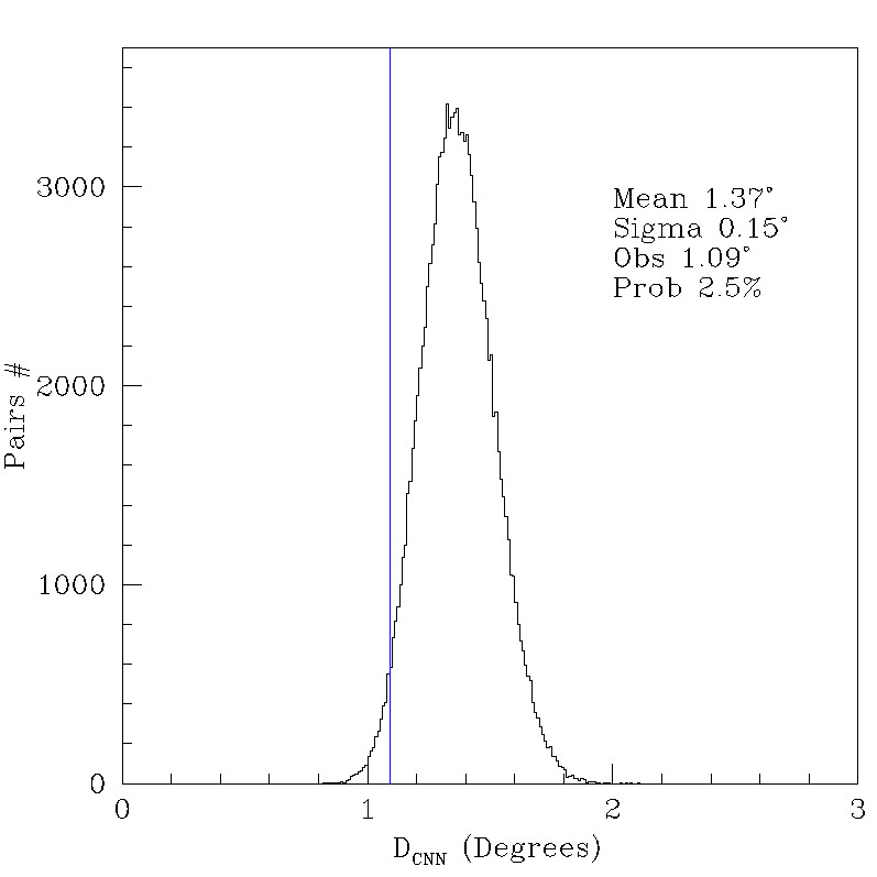
Figure 20: Distribution of $D_{\rm CNN}$ for the random sets of sources (black histogram). The histogram is well described by a Gaussian distribution with mean 1.37^∘ and standard deviation 0.15^∘. The $D_{\rm CNN}$ for our sample is shown by the blue line.

As a comparison we compute $D_{\rm CNN}$ for about 130000 sets of random new candidate sources, while keeping the cluster coordinates fixed. The coordinates of the random sources have been extracted from uniform distributions in Right Ascension and Declination. In Fig. 20, we show the distribution of $D_{\rm CNN}$ for the random sets of sources (black histogram) and for our sample (blue line). The probability of a random association between our new sources and the galaxy cluster filament is less than 2.5%. This means that the number of spurious sources related to noise, or to the Galactic foreground, is small. We verified this point with the help of mock SRT observations that we ran through the same imaging pipeline as the real ones. We find that gain fluctuations are strongly reduced in our images after the application of wavelet and denoising techniques. However, the 18-20% of the diffuse large-scale detected sources could be Galactic. A detailed description of the simulations and of the results is given in Appendix C.

If confirmed, our results reveal a new population of sources, very luminous and extended in radio, but very elusive in X-rays. These sources could be associated with the filaments of the cosmic web. The emission from these structures is believed to be very faint at all wavelengths. Indeed, we are able to detect only a fraction of them in X-rays and with low significance (1$\sigma$), while in radio we begin to detect them thanks to the high sensitivity to surface brightness of single-dish observations. The fact that most of our sample is offset to larger sizes (at the same radio power), that the average emissivity is 10-100 smaller than radio halos and relics respectively, and that the X-ray luminosity of the detected sources is about 10-100 weaker than cluster sources, are evidence that we have discovered a new population of sources at lower surface brightness. This is consistent with the thermodynamic properties of the gas in simulated cosmological filaments, whose typical X-ray emissivity is expected to be $\sim 10-100$ smaller than the emissivity of galaxy clusters with the same mass (Gheller et al., 2016).

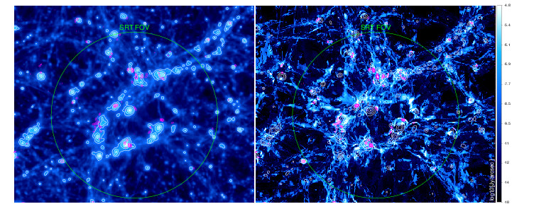
Figure 21: Left panel: estimated virial volume of all halos in the box (based on their total matter density, white contours) and detectable radio emission in the SRT observing configuration presented in this paper (purple contours) overlaid on the projected gas density (colours). Right panel: the colours show the projected full radio emission at the nominal resolution of the simulation (83 kpc/cell) and assuming this field is at $z=0.1$. The contours are the same as in the left panel. The green circles in both images represent the field of view of SRT if the simulated volume is located at $z=0.1$.

Table 6: X-ray fluxes from the regions associated with the diffuse sources in the field from RASS

Source	z	$n_{\rm H}$	$R_{200}$	$S_{\rm X}$	$D_{\rm L}$	$L_{\rm X,0.1-2.4\,keV}$
		$10^{20}$ cm-2	∘	$10^{-12}$erg s-1 cm-2	Mpc	$10^{44}$erg s-1
A1	0.104	10.6	0.18	1.2 $\pm$ 0.3	499	5.4 $\pm$ 1.4
A2	0.104	10.5	0.118	0.2 $\pm$ 0.1	499	0.7 $\pm$ 0.6
A3	0.104	11.8	0.112	0.1 $\pm$ 0.1	499	0.6 $\pm$ 0.5
B1	0.104	10.3	< 0.132	< 0.3	499	< 1.2
B2	0.1	9.01	< 0.112	< 0.1	478	< 0.5
B3	0.1	8.43	< 0.118	< 0.2	478	< 0.6
C1	0.029	10.7	< 0.292	< 0.5	132	< 0.2
C2	0.029	11.1	< 0.293	< 0.5	132	< 0.2
C3	0.029	10.7	0.323	0.9 $\pm$ 0.4	132	0.3 $\pm$ 0.1
C4	0.029	10.8	< 0.293	< 0.5	132	< 0.2
C5	0.029	10.8	< 0.288	< 0.5	132	< 0.2
C6	0.029	11.2	0.268	0.4 $\pm$ 0.3	132	0.1 $\pm$ 0.1
C7	0.1	10.2	< 0.133	< 0.3	478	< 1.1
C8	0.1	9.81	0.116	0.1 $\pm$ 0.1	478	0.6 $\pm$ 0.5
C9	0.1	9.43	< 0.13	< 0.2	478	< 1.0
C10	0.1	9.29	< 0.119	< 0.2	478	< 0.7
D1	0.1	9.74	< 0.126	< 0.2	478	< 0.9
D2	0.1	8.46	< 0.118	< 0.2	478	< 0.6
D3	0.1	8.16	< 0.112	< 0.1	478	< 0.5
E1	0.405	7.89	< 0.064	< 0.2	2283	< 14.5
E2	0.1	7.58	< 0.127	< 0.2	478	< 0.9
E3	0.1	7.42	0.117	0.1 $\pm$ 0.1	478	0.6 $\pm$ 0.5
F1	0.1	10.2	< 0.125	< 0.2	478	< 0.8
G1	0.1	7.91	< 0.123	< 0.2	478	< 0.8
G2	0.1	6.72	< 0.119	< 0.2	478	< 0.6
G3	0.1	7.53	0.119	0.2 $\pm$ 0.1	478	0.7 $\pm$ 0.5
G4	0.1	7.38	0.243	4.6 $\pm$ 0.6	478	18.5 $\pm$ 2.3
G5	0.1	7.06	0.12	0.2 $\pm$ 0.1	478	0.7 $\pm$ 0.4
G6	0.1	7.14	< 0.124	< 0.2	478	< 0.8
H1	0.1	7.77	< 0.127	< 0.2	478	< 0.9
H2	0.1	7.67	< 0.124	< 0.2	478	< 0.8
I1	0.199	5.66	0.162	3.3 $\pm$ 0.4	1011	55.8 $\pm$ 6.9
I2	0.199	5.64	< 0.086	< 0.2	1011	< 2.8
I3	0.199	5.76	0.085	0.1 $\pm$ 0.1	1011	2.6 $\pm$ 1.8
J1	0.1	7.41	< 0.125	< 0.2	478	< 0.8

Col 1: Source name; Col 2: redshift; Col 3: Hydrogen column density in the direction of the source; Col 4: $R_{200}$ of the system; Col 5: X-ray flux in the 0.5-2 keV energy band within $R_{200}$; Col 6: Luminosity distance; Col 7: X-ray luminosity in the 0.1-2.4 keV energy band within $R_{200}$.

8.1 Observations versus simulations

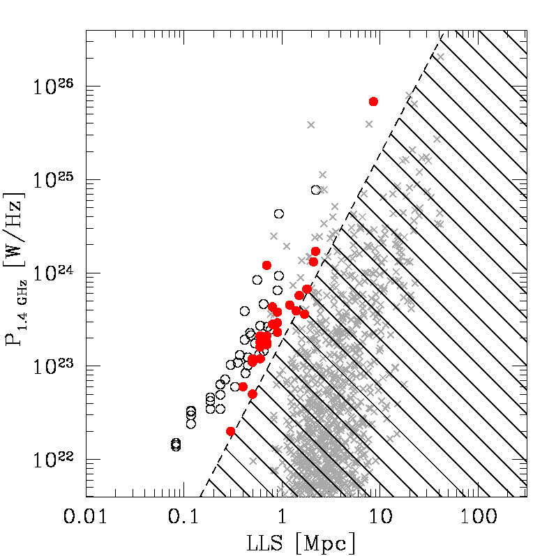
Figure 22: Radio power at 1.4 GHz versus the LLS at 1.4 GHz for the all simulated objects before the SRT observing parameters are considered (gray crosses), for simulated objects after the SRT noise and spatial resolution are applied (empty black dots), and for observed objects (full red dots). The shaded area indicates the region of the ($P_{\rm 1.4\,GHz}$, LLS) plane that cannot be accessed considering the 2$\sigma$ ($\sigma$=2.5 mJy/beam) sensitivity of the SRT+NVSS image after point source subtraction.

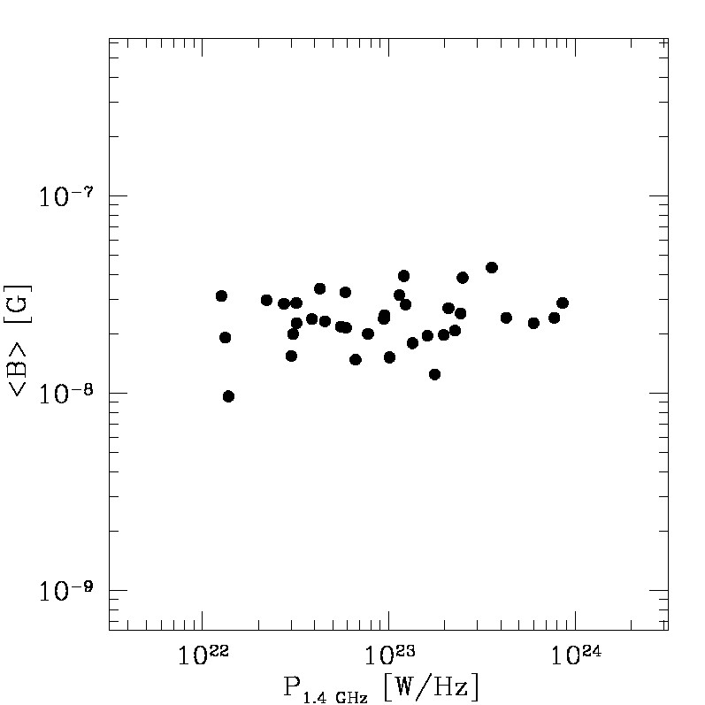
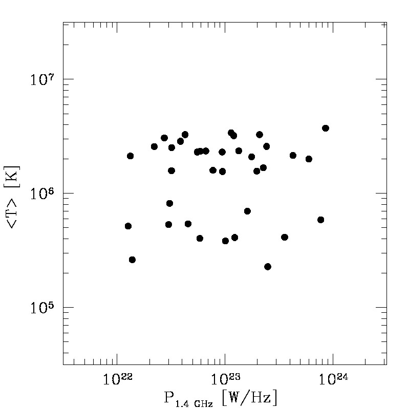
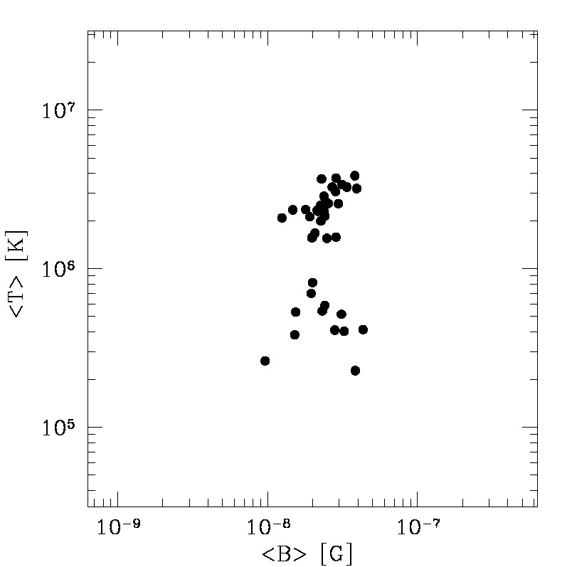
Figure 23: Top panel: mean volume-weighted magnetic field $\langle B\rangle$ versus $P_{\rm 1.4\,GHz}$. Middle panel: mean temperature $\langle T\rangle$ versus $P_{\rm 1.4\,GHz}$. Bottom panel: $\langle T\rangle$ versus $\langle B\rangle$.

To interpret our results, we compared the observations with simulations from the sample already introduced in Vazza et al. (2015) and Gheller et al. (2016), obtained with the cosmological grid code Enzo (Bryan et al., 2014). In summary, we used a uniform $1200^{3}$ grid with a resolution of 83 kpc (co-moving) to simulate the evolution of a 100 Mpc³ region from $z=30$ to $z=0$, assuming a seed magnetic field of 1 nG of primordial origin. The magnetic field in the magneto-hydro-dynamical (MHD) method uses the conservative Dedner formulation (Dedner et al., 2002) which uses hyperbolic divergence cleaning to keep $\nabla\cdot\vec{B}$ close to zero. Radiative processes and feedback from star forming regions and/or active galactic nuclei were not included in this run. The assumed cosmology is the $\Lambda$CDM cosmological model with density parameters $\Omega_{0}=1.0$, $\Omega_{\rm BM}=0.0455$, $\Omega_{\rm DM}=0.2265$ (BM and DM indicating the baryonic and the dark matter respectively).

To simulate synchrotron radio emission from the cosmic web, we followed Vazza et al. (2015) and assumed the diffusive shock acceleration of electrons at cosmological shocks, relying on the formalism by Hoeft & Brüggen (2007) to combine simulated magnetic fields and the distribution of Mach numbers, $\mathcal{M}$, in order to estimate the level of synchrotron emission across the cosmic web, which is computed for each simulated cell as:

$$P_{\nu}\propto n_{u}\xi(\mathcal{M})\cdot M^{3}c_{s}^{3}S\cdot B^{2},$$ (3)

where $n_{u}$ is the upstream gas density, $c_{s}$ is the sound speed in the upstream gas, $B$ is the magnetic field in the shocked cell, and $S$ is the shock surface. The acceleration efficiency of electrons, $\xi(\mathcal{M})$, is taken from Hoeft & Brüggen (2007) and (in the absence of seed relativistic electrons to re-accelerate) is a steep function of $\mathcal{M}$ for weak shocks, and rapidly saturates to $\xi_{\rm e}\approx 7\cdot 10^{-4}$ for $M>10$ shocks in our model.

Finally, in order to focus on the radio emission produced by filaments in our volume and minimize the contamination by denser structures along the line of sight, we relied on the filament finder presented in (Gheller et al., 2016), which allows us to extract the 3-dimensional isosurfaces associated with the mild over-densities associated with filaments, as well as to build a catalogue of single filament objects, for which mean thermodynamic and magnetic properties can be computed.

To compare with observation, we produced mock radio observation of the sky model from cosmological simulations, with a procedure similar to Vazza et al. (2015). In particular, we computed the radio emission model at 1.4 GHz (by locating our simulated box at a distance corresponding to $z=0.1$) convolving the input sky model with a final beam of 3.5${}^{\prime}\times$3.5^′ and considering a final sensitivity of 0.05 $\mu\rm Jy/arcsec^{2}$, the same as those of the image used for our analysis. The result is shown in Fig. 21. colours in the left panel represent the projected density, while in the right panel, they show the projected full radio emission at the nominal resolution of the simulation (83 kpc/cell). White contours describe the estimated virial volume of all halos in the box (based on their total matter over-density). Purple contours show the detectable radio emission in the SRT observing configuration presented in this paper.

Based on the 3-d catalogue of filaments obtained in Gheller et al. (2016), we computed the properties of filaments seen in projections in the entire volume, i.e. their total intrinsic radio power at 1.4 GHz (prior to any observational cut) and their largest linear scale. By considering the noise and resolution of the SRT observations, only a very tiny fraction ($\leq 10^{-4}$) of the radio emitting surface of the cosmic web in the simulation survives. We recomputed the corresponding radio power and largest linear size of these objects. In Fig. 22, we show the radio power at 1.4 GHz versus the LLS for all the simulated objects before the SRT observing parameters are considered (gray crosses), for simulated objects after the SRT noise and spatial resolution are applied (empty black dots), and for observed objects (full red dots). The crosses represent all the diffuse large-scale sources in the image before any observing parameter (noise and convolution) is applied. After the SRT noise and spatial resolution are taken into account, the detected sources are only those marked by empty black circles. The few detectable emission patches populate almost the same region of the ($LLS$, $P_{\rm 1.4\,GHz}$) plane as the observed candidate sources presented in this paper. In most cases, as suggested by the map in Fig. 21, these large diffuse emission regions are associated with very peripheral shocks at the crossroad between the outer virial volume of massive galaxy clusters and the filaments connecting them, which are typically detectable only in very crowded over-dense regions, similar to the high-density field observed in this work.

In Fig. 23, we show the mean magnetic field $\langle B\rangle$ and mean temperature $\langle T\rangle$ versus $P_{\rm 1.4\,GHz}$ (top and middle panels), and $\langle T\rangle$ versus $\langle B\rangle$ (bottom panel), for the simulated filaments that host emission patches which should be detectable by our SRT observation. The average properties of the host objects are typical of the most massive filaments in our simulations (Gheller et al., 2016), with $n/\langle n\rangle\sim 50-100$, $\langle B\rangle\sim 10-50$ nG, $T\sim 2\cdot 10^{5}-5\cdot 10^{6}$ K), yet the detectable regions only cover a tiny fraction (a few percent) of the filaments’ projected area, and they tend to be associated with the densest and hottest portions of filaments, connecting to the surrounding clusters. With the assumed prescription for extragalactic magnetic fields and electron acceleration at shocks, the regions which are within the range of detection in our SRT observation typically have an average magnetic field along the line of sight of $\sim 0.02-0.05\,\mu$G.

9 Summary and conclusions

In this work, we report the detection of diffuse radio emission which might be associated with a large-scale filament of the cosmic web covering a 8${}^{\circ}\times$8^∘ area in the sky, likely associated with a z$\approx$0.1 over-density traced by nine massive galaxy clusters. To investigate the presence of large-scale diffuse synchrotron emission beyond the cluster periphery, we observed this area with the Sardinia Radio Telescope. These low spatial resolution data have been combined with high resolution observations from the NRAO Very Large Array Sky Survey, to permit separation of the diffuse large-scale synchrotron emission from that of embedded discrete radio sources.

By inspecting the field of view, we identified 35 patches of diffuse emission with significance above 3$\sigma$. Two are the cluster sources already known in the direction of the galaxy clusters A523 (source A1) and A520 (source I1), five sources (C1, C6, C9, E2, and G6) are probably the leftover of the compact source subtraction process or artefacts, and the remaining 28 sources represent diffuse synchrotron radio emission with no obvious interpretation. To shed light on the nature of these new sources, we studied their radio and X-ray properties. Only eleven sources have an X-ray count rate significantly above 1$\sigma$. These sources are A1 (diffuse emission in A523), A2, A3, C3, C8, E3, G3, G4, G5, I1 (diffuse emission in A520), and I3. Apart from the two radio halos in A520 and A523, one of the significant X-ray sources (G4) sits in the $L_{\rm X,0.1-2.4\,keV}$-$P_{\rm 1.4\,GHz}$ correlation observed for radio halos and relics but has a larger size than expected for cluster sources with this power. The remaining eight sources show a X-ray luminosity between 10 and 100 times lower than expected from their radio power given the correlation observed for cluster sources, with an average X-ray luminosity of $L_{\rm X,0.1-2.4\,keV}$=0.77$\times 10^{44}$ erg/s. They populate a new region of the ($L_{\rm X,0.1-2.4\,keV}$, $P_{\rm 1.4\,GHz}$) plane that was previously unsampled.

Some of these are particularly interesting. Source A2 in combination with the source south-west of it and with Source A1 (the radio halo in A523) could represent the first case of a triple radio halo, particularly interesting because of its association with an under-luminous X-ray system. Source E1 is the largest and the more powerful diffuse radio source in the field. Its size is 25^′ and its location on the plane of the sky is in the same direction as the filament connecting A523-A525 to A509-A508. Alternatively, could be located at higher redshift, if associated with 4C +06.21, the source embedded in it. Whether this source belongs to the filament or it is instead at higher redshift has an impact on its size that ranges between 3 and 8.7 Mpc, and in the latter case it would represent the largest extragalactic diffuse synchrotron source known to date.

Overall, these objects have distinct properties from known radio halos and relics. Indeed, they show lower X-ray luminosity in the 0.1–2.4 keV band and a larger LLS than expected for a given radio power from the correlation observed for cluster sources. The mean power and the mean largest linear size of the sample (excluding the radio halos in A520 and in A523) are respectively $P_{\rm 1.4\,GHz}=2.9\times 10^{24}$ W/Hz and LLS=1.3 Mpc. The average radio emissivity and the X-ray luminosity of these sources are about 10-100 weaker than those of cluster diffuse sources. These characteristics are indicative of a very faint new population of sources. The conditional nearest neighbour distance of clusters and and candidate new sources indicates that the probability of a random association between our new sources and the galaxy cluster filament is less than 2.5%. This means that it is unlikely spurious sources related to noise or to the Galactic foreground are present. A comparison between simulations and observations shows that the radio powers and radio sizes of these sources are comparable to those expected by the brightest patches of diffuse synchrotron radio emission associated with the filaments of the cosmic web and correspond to an average magnetic field along the line of sight of $\sim 0.02-0.05\,\mu$G.

High-spatial resolution and deep radio, X-ray and optical follow-ups are essential to shed light on the nature of these puzzling sources.

Appendix A Compact sources in the field

This field of view is rich in radio sources, with a total number of thousands at 1.4 GHz. To further cross-check the flux density scale of our data, we measured the flux density of a sample of sources that satisfies the following requirements: peak brightness at 1.4 GHz larger than 200 mJy and flux larger than the 3$\sigma$ simultaneously at all frequencies (with $\sigma$ being the uncertainty in the flux measurement at the corresponding frequency). For the sake of comparison, we estimated the flux and its uncertainty over the frequency range 74 MHz - 5 GHz, by using the following observations after convolving all the images at the resolution of the GB6 ($3.6^{\prime}\times 3.4^{\prime}$):

• the VLA Low-Frequency Sky Survey Redux (VLSSr, Lane et al., 2014) at 74 MHz ($\sigma_{\rm VLSSr}=300$ mJy);

• the TIFR GMRT Sky Survey Alternative Data Release (TGSS ADR, Intema et al., 2017) at 150 MHz ($\sigma_{\rm TGSS}=50$ mJy);

• the NVSS image, at 1.4 GHz ($\sigma_{\rm NVSS}=2$ mJy);

• the combined SRT and NVSS image, at 1.4 GHz ($\sigma_{\rm SRT+NVSS}=3$ mJy);

• the Green Bank 6-cm (GB6) survey (GB6, Gregory et al., 1996) at 4.85 GHz ($\sigma_{\rm GB6}=5$ mJy).

All these data are in the Baars et al. (1977) flux scale, apart from the TGSS ADR and the VLLSr that have been calibrated according to respectively the Scaife & Heald (2012) and the Roger et al. (1973) flux density scale. Therefore, we corrected the TGSS and VLSSr fluxes accordingly. Concerning the VLSSr, we additionally increased the uncertainty in the flux measurement, as suggested by Lane et al. (2014). The flux has been evaluated by applying a cut in brightness in the NVSS image equal to 5$\sigma_{\rm NVSS}$ and by masking all the other images accordingly. This translates to a total of 24 sources. In Table 7, we report the source ID, the RA and Dec coordinates (J2000) of the peak flux in the combined SRT+NVSS image, and the peak flux as measured from the VLSSr, TGSS, NVSS, combined SRT+NVSS, GB6, along with their uncertainties that have been computed by adding in quadrature the statistic and systematic (3% of the flux) uncertainties. The flux measurements from the NVSS and the SRT+NVSS combined images have been compared to cross-check the flux scale after the combination of the data. In Fig. 24, we show the flux of the SRT+NVSS image versus the NVSS flux (dots) along with a linear fit (dashed line). The slope of the fit is 0.97, revealing a good agreement of the two flux measurements within the errors.

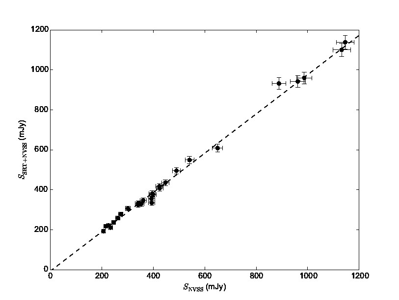
Figure 24: Flux from NVSS mosaic image versus flux from the combined SRT+NVSS image for sources with fluxes $>200$ mJy.

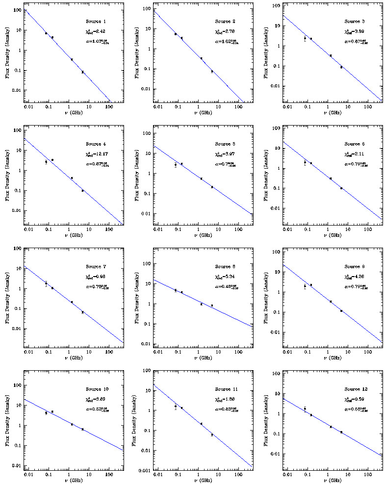
Figure 25: Flux density versus frequency for the first 12 sources in the catalogue. For each source the flux density as measured by VLSSr, TGSS, combined SRT+NVSS, and GB6 images is shown along with the power law fit, the resulting spectral index $\alpha$ value and the $\chi^{2}_{\rm red}$ of the fit.

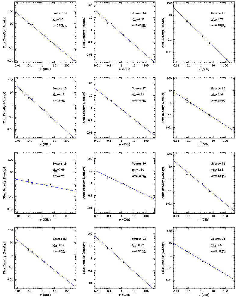
Figure 26: Flux density versus frequency for the last 12 sources in the catalogue. For each source the flux density as measured by VLSSr, TGSS, combined SRT+NVSS, and GB6 images is shown along with the power law fit, the resulting spectral index $\alpha$ value and the $\chi^{2}_{\rm red}$ of the fit.

To compare the fluxes at 1.4 GHz with the measurements at the other radio frequencies, we fit the fluxes from VLSSr, TGSS, SRT+NVSS, and GB6 versus frequency with a power law

$$S_{\nu}\propto\nu^{-\alpha},$$ (4)

where $\nu$ is the observing frequency and $\alpha$ is the spectral index. During the fitting procedure the relative errors were increased to 10% if lower than this, to take into account any systematic errors. In Table 7, we report the spectral indices values, its error and the $\chi^{2}_{\rm red}$ from the fit. All the sources have spectral index ranging from a minimum value of about 0.2 to a maximum value of about 1.1, with a mean $\alpha$=0.76 and a standard deviation $\sigma_{\alpha}$ =0.19. Plot of the flux densities versus frequency and the corresponding fits are shown in Fig. 25 and Fig. 26 for each source.

Table 7: Radio sources with peak brightness at 1.4 GHz larger than 200 mJy.

#	RA (J2000)	Dec (J2000)	$S_{\rm VLSSr}$	$S_{\rm TGSS}$	$S_{\rm NVSS}$	$S_{\rm SRT+NVSS}$	$S_{\rm GB6}$	$\alpha$	$\chi^{2}_{\rm red}$
	hms	∘:′:′′	Jy	Jy	Jy	Jy	mJy
1	5:11:37	9:31:21.40	6.8$\pm$0.6	4.3$\pm$0.2	0.39$\pm$0.01	0.33$\pm$0.01	81$\pm$10	1.07${}^{0.05}_{-0.05}$	2.42
2	5:05:32	9:26:01.79	5.3$\pm$0.6	3.4$\pm$0.1	0.35$\pm$0.01	0.33$\pm$0.01	74$\pm$10	1.02${}^{0.05}_{-0.05}$	2.78
3	5:04:31	8:27:00.24	2.4$\pm$0.7	2.3$\pm$0.1	0.34$\pm$0.01	0.32$\pm$0.01	85$\pm$12	0.87${}^{0.06}_{-0.06}$	3.89
4	5:01:58	6:50:57.71	2.6$\pm$0.6	3.3$\pm$0.1	0.42$\pm$0.01	0.42$\pm$0.01	97$\pm$10	0.87${}^{0.05}_{-0.05}$	12.17
5	5:03:03	6:09:58.82	2.7$\pm$0.7	3.1$\pm$0.2	0.54$\pm$0.02	0.55$\pm$0.02	211$\pm$14	0.70${}^{0.05}_{-0.05}$	3.97
6	4:55:38	7:52:08.42	2.0$\pm$0.6	1.8$\pm$0.1	0.30$\pm$0.01	0.31$\pm$0.01	100$\pm$11	0.79${}^{0.05}_{-0.06}$	2.11
7	5:06:10	5:22:28.42	1.8$\pm$0.5	1.1$\pm$0.1	0.23$\pm$0.01	0.21$\pm$0.01	65$\pm$10	0.78${}^{0.06}_{-0.06}$	0.98
8	4:57:07	6:45:29.63	4.7$\pm$0.8	3.7$\pm$0.2	0.89$\pm$0.03	0.93$\pm$0.03	808$\pm$28	0.48${}^{0.06}_{-0.06}$	5.34
9	5:09:07	3:48:03.21	1.9$\pm$0.6	2.2$\pm$0.1	0.34$\pm$0.01	0.33$\pm$0.01	114$\pm$10	0.79${}^{0.05}_{-0.05}$	4.26
10	5:07:35	3:08:00.44	4.1$\pm$0.8	4.8$\pm$0.2	1.13$\pm$0.03	1.10$\pm$0.03	634$\pm$23	0.52${}^{0.05}_{-0.05}$	3.89
11	5:06:37	2:37:11.02	1.6$\pm$0.5	1.3$\pm$0.1	0.22$\pm$0.01	0.22$\pm$0.01	62$\pm$9	0.83${}^{0.06}_{-0.06}$	1.88
12	5:01:45	2:24:36.45	1.7$\pm$0.5	0.9$\pm$0.1	0.23$\pm$0.01	0.22$\pm$0.01	120$\pm$10	0.58${}^{0.06}_{-0.07}$	0.59
13	4:44:40	2:48:01.22	11.0$\pm$0.8	8.6$\pm$0.3	1.15$\pm$0.03	1.14$\pm$0.03	361$\pm$16	0.83${}^{0.04}_{-0.04}$	3.20
14	4:46:22	5:41:03.56	3.3$\pm$0.7	3.3$\pm$0.2	0.40$\pm$0.01	0.38$\pm$0.01	121$\pm$13	0.87${}^{0.05}_{-0.05}$	4.82
15	4:44:17	5:01:41.76	2.9$\pm$0.5	1.8$\pm$0.1	0.21$\pm$0.01	0.19$\pm$0.01	53$\pm$9	0.98${}^{0.06}_{-0.06}$	0.77
16	4:49:08	1:52:58.99	3.7$\pm$0.6	2.9$\pm$0.1	0.40$\pm$0.01	0.38$\pm$0.01	96$\pm$10	0.90${}^{0.05}_{-0.05}$	4.16
17	4:44:18	1:54:45.61	5.5$\pm$0.7	3.7$\pm$0.2	0.65$\pm$0.02	0.61$\pm$0.02	211$\pm$13	0.79${}^{0.05}_{-0.05}$	0.83
18	4:59:43	5:20:06.76	1.7$\pm$0.6	1.0$\pm$0.1	0.25$\pm$0.01	0.24$\pm$0.01	104$\pm$10	0.65${}^{0.06}_{-0.06}$	0.04
19	5:05:22	4:59:57.84	1.9$\pm$0.6	1.2$\pm$0.1	0.99$\pm$0.03	0.96$\pm$0.03	1022$\pm$33	0.20${}^{0.01}_{-0.00}$	7.56
20	4:44:38	5:46:32.00	2.7$\pm$0.8	2.5$\pm$0.2	0.96$\pm$0.03	0.94$\pm$0.03	434$\pm$19	0.48${}^{0.05}_{-0.05}$	1.34
21	4:55:38	2:54:08.06	2.4$\pm$0.7	2.3$\pm$0.1	0.45$\pm$0.01	0.44$\pm$0.01	100$\pm$12	0.83${}^{0.05}_{-0.05}$	6.62
22	5:15:31	9:04:03.94	2.8$\pm$0.6	1.7$\pm$0.1	0.26$\pm$0.01	0.26$\pm$0.01	104$\pm$12	0.80${}^{0.06}_{-0.06}$	0.18
23	5:13:51	1:56:58.07	6.1$\pm$0.8	6.6$\pm$0.2	0.49$\pm$0.02	0.50$\pm$0.02	170$\pm$14	0.91${}^{0.04}_{-0.05}$	9.87
24	5:11:34	2:44:32.41	2.1$\pm$0.7	1.5$\pm$0.1	0.39$\pm$0.01	0.36$\pm$0.01	195$\pm$13	0.59${}^{0.06}_{-0.06}$	0.50
25	4:52:48	4:01:01.85	3.2$\pm$0.7	2.4$\pm$0.1	0.36$\pm$0.01	0.35$\pm$0.01	96$\pm$12	0.87${}^{0.06}_{-0.06}$	1.98

Col 1: Source name; Col 2 & 3: source coordinates; Col 4: Flux density from the VLSSr image at 74 MHz; Col 5: Flux density from the TGSS image at 150 MHz; Col 6: Flux density from the NVSS image at 1.4 GHz; Col 7: Flux density from the combined SRT+NVSS image at 1.4 GHz; Col 8: Flux density from the GB6 image at 4.85 GHz; Col 9: Spectral index between 74 MHz and 1.4 GHz; Col 10: Reduced chi-squared.

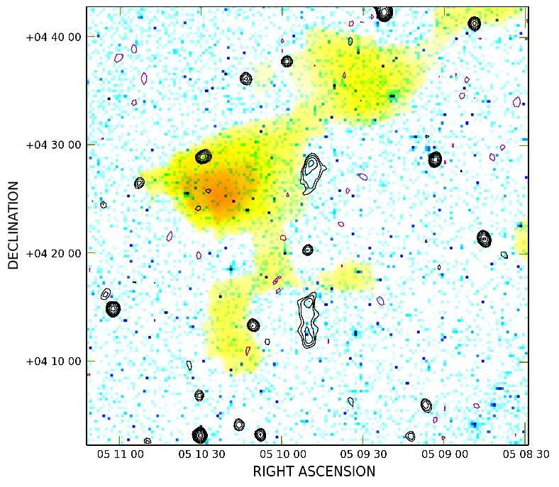
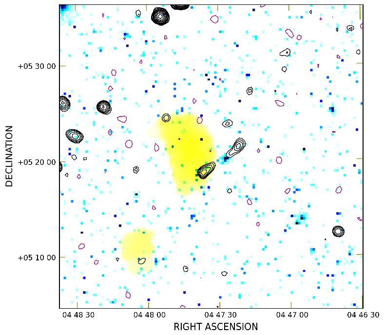
Figure 27: SRT+NVSS contours overlaid on the Planck Y-map and the optical DSS2 red image in colours (respectively yellow and blue), for the two radio galaxies (top from Region F and bottom from Region H) described in Appendix B. The contour levels are -1.35 mJy/beam, 1.35 mJy/beam (with a beam of 45^′′) and the remaining increase by a factor $\sqrt{2}$ (negative in magenta and positive in black).

Appendix B Other interesting sources

In Fig. 27, we show the SRT+NVSS contours overlaid on the SZ Y-map from the Planck satellite and the optical emission from the second Digitized Sky Survey (DSS2) red filter in the direction of two radio galaxies we serendipitously found in Region F (Fig. 13) and in Region H (Fig. 15), by inspecting the SRT+NVSS combined image. The source in the top panel of Fig. 27 is a candidate giant radio galaxy. It sits in the plane of the sky and is not present in the catalogues available in the literature. This radio source is located at RA (J2000) 05h09m50s and Dec (J2000) +04^∘20^′19^′′. Its flux density at 1.4 GHz is (46$\pm$3) mJy and its angular size is about 20^′, as measured by the combined SRT+NVSS image. On the basis of its properties, we classify it as a Fanaroff-Riley (FR) II radio galaxy with two bright hot spots and two low-brightness jets. The nucleus of this radio galaxy is clearly detected, while the optical emission is below the noise level. Since radio galaxies are usually giant elliptical galaxies with absolute magnitude of at least -19 and the limiting apparent magnitude of the optical DSS2 red filter is 20.8, we derive that the source distance is larger than 0.9 Gpc. Considering that the angular size has a minimum for z=1, we infer that the size of this source ranges between 4 and 10 Mpc. Interestingly, the SZ Y-map reveal hints of cavities at the location of the lobes of the source.

The source in the bottom panel of Fig. 27 is another interesting source, located at RA (J2000) 04h47m23.9s Dec (J2000) +05d18m50s. It has a flux density at 1.4 GHz of (19$\pm$1) mJy and its angular size is about 6^′, as measured by the combined SRT+NVSS image. The closest systems with optical identification have a redshift z$\approx$0.1. At this distance, the source would have a linear size of about 700 kpc. We classify it as a FRII radio galaxy.

Appendix C Effects of gain fluctuations and Galactic foreground

Gain fluctuations of the receiving chain can affect the observed radio emission. To exclude that the new candidate sources are spurious patches of radio emission due to these gain fluctuations, we produced two 8${}^{\circ}\times$8^∘ RA-DEC mock SRT observations of the sky and run them through the same imaging pipeline as the observations. To reduce the computational burden, the simulations were run only in the same frequency ranges as the NVSS (1364.9-1414.9 MHz and 1435.1-1485.1 MHz) and then averaged.

As a first step, we characterize the noise properties of our images. For each $8^{\circ}\times 8^{\circ}$ RA-DEC observation and each polarization, we extracted 5 streams of data-points along the full sub-scan in cold regions of the sky. The total number of data points for each stream is about 850 and they have been acquired every 100 ms corresponding to a sub-scan duration of about 85 s. For each data stream we derived the power spectrum of the noise fluctuations in the frequency range 0.01-5 Hz and all the power spectra were averaged, see Fig. 28. We interpreted the average observed noise spectrum as a combination of white noise with power spectrum $P_{\rm white}\simeq 1\,$(Jy/beam)²/Hz² corresponding, according to the radiometer equation, to a system temperature of 33 K, for an integration time of 100 ms, and a bandwidth of 50 MHz, and a 1/f-noise with power

$$P_{1/f}=P_{0}(f/f_{\rm 0})^{-s},$$ (5)

where $P_{0}=3$(Jy/beam)²/Hz², $f_{\rm 0}=1$ Hz, and $s=1.8$. In Fig. 28, we show the observed power spectrum of the noise (blue), the white-noise (horizontal red dashed) component, the f-noise (diagonal red dashed) component, and the sum of the white and 1/f noise (red continuous line).

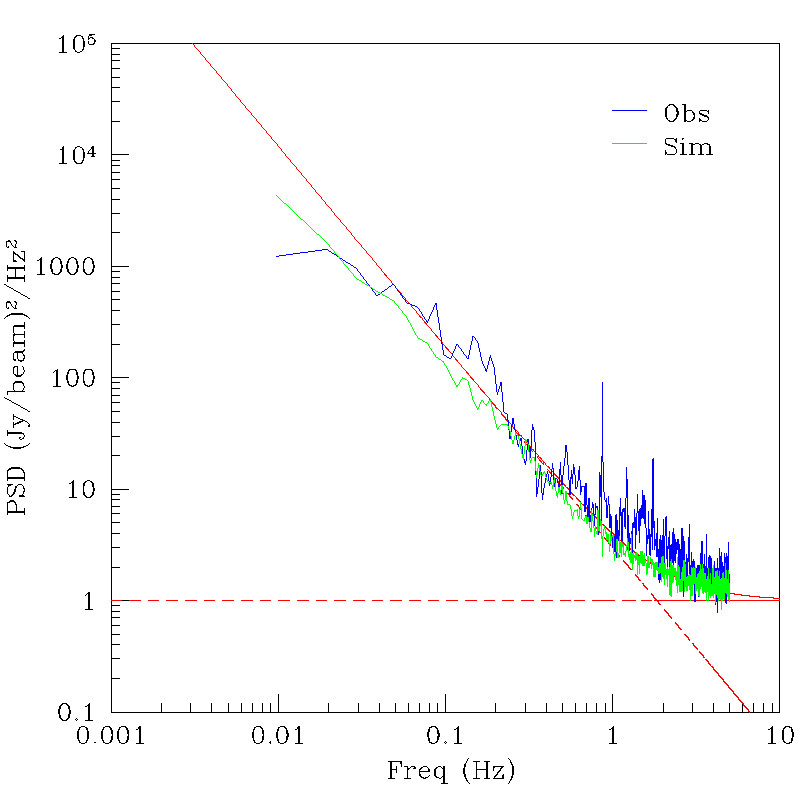
Figure 28: Power spectrum of the noise derived from the observations (blue) and from the simulations (green). The horizontal and diagonal red dashed lines represent respectively the white-noise and 1/f-noise components, while the red continuous line is the sum of white and 1/f-noise.

To investigate whether these gain fluctuations can produce spurious large-scale radio emission, we produced mock observations with the same noise properties as the observations and a point-like source sky model. We assumed a system temperature $T_{\rm sys}=33$ K, a gain $G=0.47$ K/Jy, a forward efficiency $\eta_{\rm F}=1$, and a flat gain curve (see Bolli et al., 2015). We adopted a ground temperature $T_{\rm ground}=303$ K and a zenith opacity $\tau=0.006$, as registered at the time of our observations. The sky model has been obtained from the NVSS by applying a cut in brightness of 10$\sigma_{\rm NVSS}=4.5\,$mJy/beam. The image has been convolved to the SRT resolution at the NVSS frequency (13.66^′). In Fig. 28, we show for consistency the averaged power spectrum of the noise derived from the mock data in green. At high frequencies, the observed power spectral density is slightly higher than the mock one. This is probably due to the fact that the mock data do not include the confusion noise, naturally present in the observations.

In Fig. 29, we compare the model to the images obtained after the pipeline: the model of the sky is shown in the top-left panel, the image derived by direct averaging all the RA and DEC baseline subtracted scans in the top-right panel, the image after mixing and denoising algorithms in the bottom-left panel, and the difference of the last two in the bottom-right panel. The top-right and bottom-left panels show that gain fluctuations are present along the sub-scan direction (with auto-correlation length of about 10 s) but appear to be completely de-correlated between a sub-scan and those immediately before and after. After mixing and denoising, these small-scale fluctuations are strongly reduced. This analysis indicates that the new candidate sources are not the result of gain fluctuations of the receiving system.

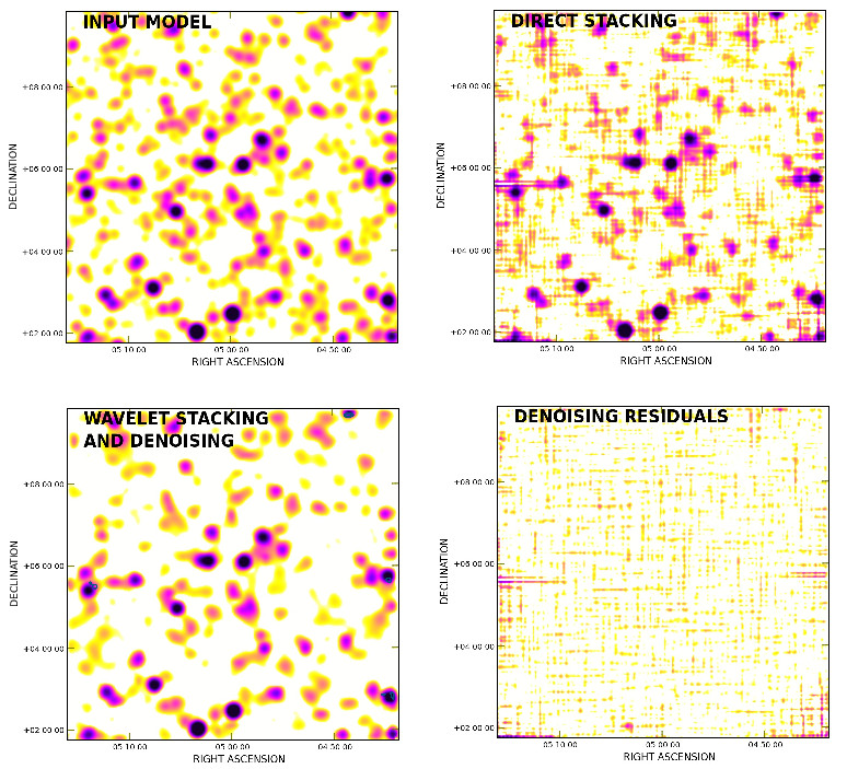
Figure 29: Top-left panel: model of the sky including only the point-like sources. Top-right panel: the image derived by direct averaging all the RA and DEC baseline subtracted scans. Bottom-left panel: image after applying the wavelet stacking and denoising algorithms. The blue contours represent the difference between the wavelet stacking and denoising image and the input model and start from 3$\sigma$ of the first. Bottom-right panel: difference of the last two panels.

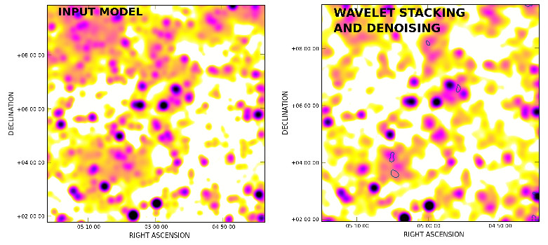
Figure 30: Left panel: model of the sky including the point-like sources and a model of our Galaxy foreground. Right panel: The colours represent the radio emission obtained by applying the imaging pipeline to mock observations including a Galactic and a point-like source contribution. Blue contours show the diffuse synchrotron patches after the NVSS point-like source model has been subtracted and start from 3$\sigma$ of the wavelet stacking and denoising image.

To investigate whether these sources could be of Galactic origin, we repeated the same procedure after including the Galactic contribution in the model. We produced the mock Galactic emission by using a power spectrum derived from the Stockert survey (Reich, 1982) around the field of interest. The Stockert survey has a resolution of 35^′, coarser than the SRT. The power spectrum of the Galactic foreground estimated from the Stockert survey has been extrapolated down to the cell-size of the Stockert image (15^′, comparable to the SRT resolution). Moreover, it should be noted that most of the power is on large scales. The mock Galactic emission was added to the NVSS point-like source model described before. In Fig. 30, we show on the left the model and on the right the image after using the same pipeline as for the observations in colours, while in contours the diffuse synchrotron patches after the NVSS point-like source model has been subtracted. Apart from structures at the edges of the image, five patches survive in the final image. Therefore, we conclude that only about 18-20% of the new candidate sources we discover could be of Galactic origin.

References

- Baars et al. (1977) Baars, J. W. M., Genzel, R., Pauliny-Toth, I. I. K., & Witzel, A. 1977, A&A, 61, 99
- Bagchi et al. (2002) Bagchi, J., Enßlin, T. A., Miniati, F., et al. 2002, New Astron., 7, 249
- Baiesi-Pillastrini et al. (1984) Baiesi-Pillastrini, G. C., Palumbo, G. G. C., & Vettolani, G. 1984, A&AS, 56, 363
- Böhringer et al. (2000) Böhringer, H., Voges, W., Huchra, J. P., et al. 2000, ApJS, 129, 435
- Bolli et al. (2015) Bolli, P., Orlati, A., Stringhetti, L., et al. 2015, Journal of Astronomical Instrumentation , 4, 1550008-880
- Bonafede et al. (2009) Bonafede, A., Feretti, L., Giovannini, G., et al. 2009, A&A, 503, 707
- Bonafede et al. (2014) Bonafede, A., Intema, H. T., Brüggen, M., et al. 2014, MNRAS, 444, L44
- Boschin et al. (2013) Boschin, W., Girardi, M., & Barrena, R. 2013, MNRAS, 434, 772
- Brown et al. (2017) Brown, S., Vernstrom, T., Carretti, E., et al. 2017, MNRAS, 468, 4246
- Brüggen et al. (2005) Brüggen, M., Ruszkowski, M., Simionescu, A., Hoeft, M., & Dalla Vecchia, C. 2005, ApJ, 631, L21
- Bryan et al. (2014) Bryan, G. L., Norman, M. L., O’Shea, B. W., et al. 2014, ApJS, 211, 19
- Carretti et al. (2013) Carretti, E., Brown, S., Staveley-Smith, L., et al. 2013, MNRAS, 430, 1414
- Cavagnolo et al. (2008) Cavagnolo, K. W., Donahue, M., Voit, G. M., & Sun, M. 2008, ApJ, 682, 821-834
- Cen & Ostriker (1999) Cen, R., & Ostriker, J. P. 1999, ApJ, 514, 1
- Chow-Martínez et al. (2014) Chow-Martínez, M., Andernach, H., Caretta, C. A., & Trejo-Alonso, J. J. 2014, MNRAS, 445, 4073
- Colberg et al. (2005) Colberg, J. M., Krughoff, K. S., & Connolly, A. J. 2005, MNRAS, 359, 272
- Condon et al. (1998) Condon, J. J., Cotton, W. D., Greisen, E. W., et al. 1998, AJ, 115, 1693
- Crawford et al. (1995) Crawford, C. S., Edge, A. C., Fabian, A. C., et al. 1995, MNRAS, 274, 75
- Davé et al. (2001) Davé, R., Cen, R., Ostriker, J. P., et al. 2001, ApJ, 552, 473
- David et al. (1996) David, L. P., Jones, C., & Forman, W. 1996, ApJ, 473, 692
- de Graaff et al. (2017) de Graaff, A., Cai, Y.-C., Heymans, C., & Peacock, J. A. 2017, arXiv:1709.10378
- Dedner et al. (2002) Dedner, A., Kemm, F., Kröner, D., et al. 2002, Journal of Computational Physics, 175, 645
- Dickey & Lockman (1990) Dickey, J. M., & Lockman, F. J. 1990, ARA&A, 28, 215
- Drinkwater et al. (1997) Drinkwater, M. J., Webster, R. L., Francis, P. J., et al. 1997, MNRAS, 284, 85
- Eckert et al. (2015) Eckert, D., Jauzac, M., Shan, H., et al. 2015, Nature, 528, 105
- Einasto et al. (2001) Einasto, M., Einasto, J., Tago, E., Müller, V., & Andernach, H. 2001, AJ, 122, 2222
- Farnsworth et al. (2013) Farnsworth, D., Rudnick, L., Brown, S., & Brunetti, G. 2013, ApJ, 779, 189
- Fatigoni (2017) Sofia Fatigoni, Master thesis of, A.A. 2016/2017, Mapping the microwave emission of Andromeda: filling the gap between IR and Radio emission, Università La Sapienza (Rome, Italy)
- Feretti et al. (2012) Feretti, L., Giovannini, G., Govoni, F., & Murgia, M. 2012, A&ARv, 20, 54
- Finoguenov et al. (2007) Finoguenov, A., Guzzo, L., Hasinger, G., et al. 2007, ApJS, 172, 182
- Gal et al. (2000) Gal, R. R., de Carvalho, R. R., Brunner, R., Odewahn, S. C., & Djorgovski, S. G. 2000, AJ, 120, 540
- Gehrels (1986) Gehrels, N. 1986, ApJ, 303, 336
- Gheller et al. (2016) Gheller, C., Vazza, F., Brüggen, M., et al. 2016, MNRAS, 462, 448
- Giovannini et al. (1999) Giovannini, G., Tordi, M., & Feretti, L. 1999, New Astron., 4, 141
- Giovannini & Feretti (2000) Giovannini, G., & Feretti, L. 2000, New Astron., 5, 335
- Giovannini et al. (2010) Giovannini, G., Bonafede, A., Feretti, L., Govoni, F., & Murgia, M. 2010, A&A, 511, L5
- Giovannini et al. (2011) Giovannini, G., Feretti, L., Girardi, M., et al. 2011, A&A, 530, L5
- Giovannini et al. (2013) Giovannini, G., Vacca, V., Girardi, M., et al. 2013, MNRAS, 435, 518
- Girardi et al. (1997) Girardi, M., Escalera, E., Fadda, D., et al. 1997, ApJ, 482, 41
- Girardi et al. (2008) Girardi, M., Barrena, R., Boschin, W., & Ellingson, E. 2008, A&A, 491, 379
- Girardi et al. (2016) Girardi, M., Boschin, W., Gastaldello, F., et al. 2016, MNRAS, 456, 2829
- Govoni et al. (2001) Govoni, F., Feretti, L., Giovannini, G., et al. 2001, A&A, 376, 803
- Govoni et al. (2004) Govoni, F., Markevitch, M., Vikhlinin, A., et al. 2004, ApJ, 605, 695
- Govoni et al. (2005) Govoni, F., Murgia, M., Feretti, L., et al. 2005, A&A, 430, L5
- Govoni et al. (2006) Govoni, F., Murgia, M., Feretti, L., et al. 2006, A&A, 460, 425
- Govoni et al. (2017) Govoni, F., Murgia, M., Vacca, V., et al. 2017, A&A, 603, A122
- Gregory et al. (1996) Gregory, P. C., Scott, W. K., Douglas, K., & Condon, J. J. 1996, ApJS, 103, 427
- Haines et al. (2017) Haines, C. P., Finoguenov, A., Smith, G. P., et al. 2017, arXiv:1709.04945
- Hoeft & Brüggen (2007) Hoeft, M., & Brüggen, M. 2007, MNRAS, 375, 77
- Hurier et al. (2013) Hurier, G., Macías-Pérez, J. F., & Hildebrandt, S. 2013, A&A, 558, A118
- Ikebe et al. (2002) Ikebe, Y., Reiprich, T. H., Böhringer, H., Tanaka, Y., & Kitayama, T. 2002, A&A, 383, 773
- Intema et al. (2017) Intema, H. T., Jagannathan, P., Mooley, K. P., & Frail, D. A. 2017, A&A, 598, A78
- Kettula et al. (2015) Kettula, K., Giodini, S., van Uitert, E., et al. 2015, MNRAS, 451, 1460
- Kronberg et al. (2007) Kronberg, P. P., Kothes, R., Salter, C. J., & Perillat, P. 2007, ApJ, 659, 267
- Lane et al. (2014) Lane, W. M., Cotton, W. D., van Velzen, S., et al. 2014, MNRAS, 440, 327
- Loi et al. (2017) Loi, F., Murgia, M., Govoni, F., et al. 2017, arXiv:1708.07125
- Macario et al. (2014) Macario, G., Intema, H. T., Ferrari, C., et al. 2014, A&A, 565, A13
- Mahdavi et al. (2007) Mahdavi, A., Hoekstra, H., Babul, A., Balam, D. D., & Capak, P. L. 2007, ApJ, 668, 806
- Mann & Ebeling (2012) Mann, A. W., & Ebeling, H. 2012, MNRAS, 420, 2120
- Markevitch et al. (2005) Markevitch, M., Govoni, F., Brunetti, G., & Jerius, D. 2005, ApJ, 627, 733
- Melis et al. (2018) Melis, A. et al. 2018, SArdinia Roach2-based Digital Architecture for Radio Astronomy (SARDARA), Journal of Astronomical Instrumentation, Vol. 7, No. 1, 1850004 (17 pages)
- Murgia et al. (2004) Murgia, M., Govoni, F., Feretti, L., et al. 2004, A&A, 424, 429
- Murgia et al. (2009) Murgia, M., Govoni, F., Markevitch, M., et al. 2009, A&A, 499, 679
- Murgia et al. (2010) Murgia, M., Govoni, F., Feretti, L., & Giovannini, G. 2010, A&A, 509, A86
- Murgia et al. (2016) Murgia, M., Govoni, F., Carretti, E., et al. 2016, MNRAS, 461, 3516
- Okabe & Miki (1984) Okabe, A. and Miki, F., "A Conditional Nearest-Neighbor Spatial Association Measure for the Analysis of Conditional Locational Interdependence", Environment and Planning A, Vol.16, pp.163-171
- Orrú et al. (2007) Orrú, E., Murgia, M., Feretti, L., et al. 2007, A&A, 467, 943
- Ostrander et al. (1998) Ostrander, E. J., Nichol, R. C., Ratnatunga, K. U., & Griffiths, R. E. 1998, AJ, 116, 2644
- Perley & Butler (2013) Perley, R. A., & Butler, B. J. 2013, ApJS, 204, 19
- Piffaretti et al. (2011) Piffaretti, R., Arnaud, M., Pratt, G. W., Pointecouteau, E., & Melin, J.-B. 2011, A&A, 534, A109
- Pizzo et al. (2008) Pizzo, R. F., de Bruyn, A. G., Feretti, L., & Govoni, F. 2008, A&A, 481, L91
- Planck Collaboration et al. (2013) Planck Collaboration, Ade, P. A. R., Aghanim, N., et al. 2013, A&A, 550, A134
- Planck Collaboration et al. (2014) Planck Collaboration, Ade, P. A. R., Aghanim, N., et al. 2014, A&A, 571, A16
- Planck Collaboration et al. (2016a) Planck Collaboration, Aghanim, N., Arnaud, M., et al. 2016, A&A, 594, A22
- Planck Collaboration et al. (2016b) Planck Collaboration, Ade, P. A. R., Aghanim, N., et al. 2016, A&A, 594, A27
- Prandoni et al. (2017) Prandoni, I., Murgia, M., Tarchi, A., et al. 2017, arXiv:1703.09673
- Reich (1982) Reich, W. 1982, A&AS, 48, 219
- Reiprich & Böhringer (2002) Reiprich, T. H., & Böhringer, H. 2002, ApJ, 567, 716
- Rines et al. (2003) Rines, K., Geller, M. J., Kurtz, M. J., & Diaferio, A. 2003, AJ, 126, 2152
- Roger et al. (1973) Roger, R. S., Costain, C. H., & Bridle, A. H. 1973, AJ, 78, 1030
- Ryu et al. (2008) Ryu, D., Kang, H., Cho, J., & Das, S. 2008, Science, 320, 909
- Scaife & Heald (2012) Scaife, A. M. M., & Heald, G. H. 2012, MNRAS, 423, L30
- Sommer et al. (2017) Sommer, M. W., Basu, K., Intema, H., et al. 2017, MNRAS, 466, 996
- Struble & Rood (1999) Struble, M. F., & Rood, H. J. 1999, ApJS, 125, 35
- Subramanian (2016) Subramanian, K. 2016, Reports on Progress in Physics, 79, 076901
- Vacca et al. (2010) Vacca, V., Murgia, M., Govoni, F., et al. 2010, A&A, 514, A71
- Vacca et al. (2014) Vacca, V., Feretti, L., Giovannini, G., et al. 2014, A&A, 561, A52
- Valente et al. (2010) Valente, G., Pisanu, T., Bolli, P., et al. 2010, Proc. SPIE, 7741, 774126
- van Weeren et al. (2013) van Weeren, R. J., Fogarty, K., Jones, C., et al. 2013, ApJ, 769, 101
- Van Weeren et al. (2016) Van Weeren, R. J., Andrade-Santos, F., Dawson, W., et al. 2016, American Astronomical Society Meeting Abstracts, 227, 202.09
- Vazza et al. (2014) Vazza, F., Brüggen, M., Gheller, C., & Wang, P. 2014, MNRAS, 445, 3706
- Vazza et al. (2015) Vazza, F., Ferrari, C., Brüggen, M., et al. 2015, A&A, 580, A119
- Venturi et al. (2017) Venturi, T., Rossetti, M., Brunetti, G., et al. 2017, A&A, 603, A125
- Vernstrom et al. (2017) Vernstrom, T., Gaensler, B. M., Brown, S., Lenc, E., & Norris, R. P. 2017, MNRAS, 467, 4914
- Veron-Cetty & Veron (1996) Veron-Cetty, M.-P., & Veron, P. 1996, ESO Scientific Report, Garching: European Southern Observatory (ESO), |c1996, 7th ed.
- Voges et al. (1999) Voges, W., Aschenbach, B., Boller, T., et al. 1999, A&A, 349, 389
- Xu & Han (2014) Xu, J., & Han, J. L. 2014, MNRAS, 442, 3329
- Zwicky et al. (1965) Zwicky, F., Karpowicz, M., & Kowal, C. T. 1965, “Catalogue of Galaxies and of Clusters of Galaxies”, 1965, Volume V Pasadena: California Institute of Technology, CGCG5“