A Duality-Based Approach for Distributed Optimization with Coupling Constraints

Abstract

In this paper we consider a distributed optimization scenario in which a set of agents has to solve a convex optimization problem with separable cost function, local constraint sets and a coupling inequality constraint. We propose a novel distributed algorithm based on a relaxation of the primal problem and an elegant exploration of duality theory. Despite its complex derivation based on several duality steps, the distributed algorithm has a very simple and intuitive structure. That is, each node solves a local version of the original problem relaxation, and updates suitable dual variables. We prove the algorithm correctness and show its effectiveness via numerical computations.

1 Introduction

A common set-up in large-scale optimization consists in minimizing the sum of local cost functions, each one depending on a local variable, subject to a constraint coupling the local decision variables. This optimization structure arises in several concrete problems as, e.g., in resource allocation problems (e.g., in Communications or Robotics) or energy flow optimization in smart grids. Solutions in a parallel, master-subproblem architecture have been known for a while, see, e.g., (Bertsekas and Tsitsiklis, 1989). More recently Tran-Dinh et al. (2016) propose a parallel inexact dual decomposition scheme combined with smoothing techniques for solving these separable convex optimization problems.

In the last years a new distributed computation paradigm has been investigated to solve optimization problems arising in a network context. Since the above mentioned class of optimization problems has important applications in network scenarios, proposing distributed algorithms is subject of great interest. This class of problems has been addressed in a distributed set-up in (Bürger et al., 2014), where a cutting-plane consensus scheme is proposed to solve the dual problem. The idea is to iteratively approximate a local problem with linear constraints (cutting planes) and exchange the active ones with neighboring nodes. A similar approach was applied in (Bürger et al., 2013) to design a distributed model predictive control scheme. Simonetto and Jamali-Rad (2016) propose a consensus-based distributed algorithm to generate approximate dual solutions for this class of problems. This distributed optimization set-up is also addressed by Falsone et al. (2016). A consensus-based proximal minimization on the dual problem is proposed to generate a dual solution. In these last two papers a primal recovery mechanism is proposed to obtain a primal optimal solution. A special coupling is considered in (Notarnicola et al., 2016), where a preliminary version of the idea proposed in this paper is applied to a min-max optimization problem for demand side management. Chang (2016) considers problems with a linear coupling constraint and proposes a proximal dual consensus ADMM to solve it in a distributed way. Chang et al. (2014) propose a consensus-based primal-dual perturbation algorithm to solve optimization problems with a slightly more general cost function (a coupling term known to all agents is allowed). Mateos-Núñez and Cortés (2015) address a class of min-max optimization problems which are strictly related to the same problem set-up investigated in this paper. They solve the min-max problem through a Laplacian-based saddle-point subgradient scheme.

The main paper contribution is the design of a novel distributed method, based on relaxation and duality, to solve convex optimization problems with separable cost function and coupling constraint. The proposed algorithm is based on two main methodological approaches. First, we consider a relaxation of the primal problem by constraining its dual with an additional box constraint. Such a dual is shown to have the same dual (and then primal) cost if the bound is sufficiently large. We show that without such a relaxation the algorithmic idea is not guaranteed to be implementable. Second, we apply duality on a series of equivalent problems. Specifically, we generate an equivalent version of the box-constrained dual problem in order to enforce the graph sparsity. By applying dual decomposition another dual problem is introduced. This final problem has a sparse structure, so that a subgradient algorithm applied to it turns out to be a distributed algorithm. In order to explicitly compute a local subgradient at each node, a further duality step is performed on the local subproblem, thus obtaining an optimization problem in the original primal variables. Despite this lengthy and complex duality tour, the resulting distributed algorithm has a simple and clean structure: each node finds a primal-dual optimal solution pair of a relaxed, local version of the original primal problem, and linearly updates some additional local dual variables.

The outline of the paper is as follows. In Section 2 we formalize the distributed optimization set-up and give some preliminaries. In Section 3 we show a first attempt to design a distributed algorithm, which turns out not to be implementable. In Section 4 we introduce the relaxation approach, derive our distributed optimization algorithm, and analyze it. In Section 5 we corroborate the theoretical results with a numerical example.

2 Distributed Optimization Set-up and Preliminaries

In this section we set-up the distributed optimization framework and recall useful preliminaries on duality.

2.1 Distributed optimization set-up

Consider the following optimization problem

$$\begin{split}\min_{\mathbf{x}_{1},\ldots,\mathbf{x}_{N}}\>&\>\textstyle\sum\limits_{i=1}^{N}f_{i}(\mathbf{x}_{i})\\ \text{subj. to}\>&\>\mathbf{x}_{i}\in X_{i},\hskip 42.67912pti\in\{1,\ldots,N\}\\ &\>\textstyle\sum\limits_{i=1}^{N}g_{i}(\mathbf{x}_{i})\preceq 0\end{split}$$ (1)

where for all $i\in\{1,\ldots,N\}$, the set $X_{i}\subseteq^{n_{i}}$ with $n_{i}\in{\mathbb{N}}$, the functions $f_{i}:^{n_{i}}\rightarrow$ and $g_{i}:^{n_{i}}\rightarrow^{S}$ with $S\in{\mathbb{N}}$.

Assumption 2.1

For all $i\in\{1,\ldots,N\}$, each function $f_{i}$ is convex, and each $X_{i}$ is a non-empty, compact, convex set. Moreover, for all $s\in\{1,\ldots,S\}$ each component $g_{is}:^{n_{i}}\rightarrow$ of $g_{i}$ is a convex function.

The following assumption is the well-known Slater’s constraint qualification.

Assumption 2.2

There exist $\bar{\mathbf{x}}_{1}\in X_{1},\ldots,\bar{\mathbf{x}}_{N}\in X_{N}$ such that $\sum_{i=1}^{N}g_{i}(\bar{\mathbf{x}}_{i})\prec\mathbf{0}$. $\square$

We consider a network of $N$ processors communicating according to a connected, undirected graph $\mathcal{G}=(\{1,\ldots,N\},\mathcal{E})$, where $\mathcal{E}\subseteq\{1,\ldots,N\}\times\{1,\ldots,N\}$ is the set of edges. Edge $(i,j)$ models the fact that node $i$ sends information to $j$. Note that, since we assume the graph to be undirected, for each $(i,j)\in\mathcal{E}$, then also $(j,i)\in\mathcal{E}$. We denote by $|\mathcal{E}|$ the cardinality of $\mathcal{E}$ and by $\mathcal{N}_{i}$ the set of neighbors of node $i$ in $\mathcal{G}$, i.e., $\mathcal{N}_{i}:=\left\{j\in\{1,\ldots,N\}\mid(i,j)\in\mathcal{E}\right\}$.

2.2 Preliminaries on Optimization and Duality

Consider a constrained optimization problem, addressed as primal problem, having the form

$$\begin{split}\min_{z\in Z}\>&\>f(z)\\ \text{subj. to}\>&\>g(z)\preceq 0\end{split}$$ (2)

where $Z\subseteq^{N}$ is a convex and compact set, $f:^{N}\rightarrow$ is a convex function and $g:^{N}\rightarrow^{S}$ is such that each component $g_{s}:^{N}\rightarrow$, $s\in\{1,\ldots,S\}$, is a convex function.

The following optimization problem

$$\begin{split}\max_{\mu}\>&\>q(\mu)\\ \text{subj. to}\>&\>\mu\succeq 0\end{split}$$ (3)

is called the dual of problem (2), where $q:^{S}\rightarrow$ is obtained by minimizing with respect to $z\in Z$ the Lagrangian function $\mathcal{L}(z,\mu):=f(z)+\mu^{\top}g(z)$, i.e., $q(\mu)=\min_{z\in Z}\mathcal{L}(z,\mu)$. Problem (3) is well posed since the domain of $q$ is convex and $q$ is concave on its domain.

It can be shown that the following inequality holds

$$\operatornamewithlimits{inf\vphantom{p}}_{z\in Z}\sup_{\mu\succeq 0}\mathcal{L}(z,\mu)\geq\sup_{\mu\succeq 0}\operatornamewithlimits{inf\vphantom{p}}_{z\in Z}\mathcal{L}(z,\mu),$$ (4)

which is called weak duality. When in (4) the equality holds, then we say that strong duality holds and, thus, solving the primal problem (2) is equivalent to solving its dual formulation (3). In this case the right-hand-side problem in (4) is referred to as saddle-point problem of (2).

Definition 2.3

A pair $(z^{\star},\mu^{\star})$ is called a primal-dual optimal solution of problem (2) if $z^{\star}\in Z$ and $\mu^{\star}\succeq 0$, and $(z^{\star},\mu^{\star})$ is a saddle point of the Lagrangian, i.e.,

$$\mathcal{L}(z^{\star},\mu)\leq\mathcal{L}(z^{\star},\mu^{\star})\leq\mathcal{L}(z,\mu^{\star})$$

for all $z\in Z$ and $\mu\succeq 0$. $\square$

A more general min-max property can be stated. Let $Z\subseteq^{N}$ and $W\subseteq^{S}$ be nonempty convex sets. Let $\phi:Z\times W\to$, then the following inequality

$$\operatornamewithlimits{inf\vphantom{p}}_{z\in Z}\sup_{w\in W}\phi(z,w)\geq\sup_{w\in W}\operatornamewithlimits{inf\vphantom{p}}_{z\in Z}\phi(z,w)$$

holds true and is called the max-min inequality. When the equality holds, then we say that $\phi$, $Z$ and $W$ satisfy the strong max-min property or the saddle-point property.

The following theorem gives a sufficient condition for the strong max-min property to hold.

Proposition 2.4 ((Bertsekas, 2009, Propositions 4.3))

Let $\phi$ be such that (i) $\phi(\cdot,w):Z\rightarrow$ is convex and closed for each $w\in W$, and (ii) $-\phi(z,\cdot):W\rightarrow$ is convex and closed for each $z\in Z$. Assume further that $W$ and $Z$ are convex compact sets. Then $\sup_{w\in W}\operatornamewithlimits{inf\vphantom{p}}_{z\in Z}\phi(z,w)=\operatornamewithlimits{inf\vphantom{p}}_{z\in Z}\sup_{w\in W}\phi(z,w)$ and the set of saddle points is nonempty and compact.  $\square$

3 Towards A Distributed Optimization Algorithm

In this section we provide a first attempt to design a duality-based distributed algorithm to solve problem (1), but then show that in general it is not guaranteed to be implementable.

3.1 A First Dual Problem Derivation

We start by deriving the equivalent dual problem of (1) as formally stated in the next lemma.

Lemma 3.1

Let Assumptions 2.1 and 2.2 hold. The optimization problem

$$\begin{split}\max_{\boldsymbol{\mu}\in^{S}}\>&\>\textstyle\sum\limits_{i=1}^{N}q_{i}(\boldsymbol{\mu})\\ \text{subj. to}\>&\>\boldsymbol{\mu}\succeq\mathbf{0}\end{split}$$ (5)

with

$$q_{i}(\boldsymbol{\mu}):=\min_{\mathbf{x}_{i}\in X_{i}}\Big{(}f_{i}(\mathbf{x}_{i})+\boldsymbol{\mu}^{\top}g_{i}(\mathbf{x}_{i})\Big{)},$$ (6)

for all $i\in\{1,\ldots,N\}$, is the dual of problem (1). Moreover, both problems (1) and (5) have finite optimal cost, respectively $f^{\star}$ and $q^{\star}$, and strong duality holds, i.e., $f^{\star}=q^{\star}$.  $\square$

The proof of this lemma is omitted for the sake of space, but can be shown by using classical methods from duality theory.

Remark 3.2

Since $q(\boldsymbol{\mu})=\sum_{i=1}^{N}q_{i}(\boldsymbol{\mu})$ is the dual function of (1), it is concave on its convex domain, which can be shown to be the entire $\boldsymbol{\mu}\succeq\mathbf{0}$. $\square$

3.2 Tentative Distributed Dual Subgradient

We focus now on the solution of problem (5). In order to make problem (5) amenable for a distributed solution, we need to enforce a sparsity structure. To this end, we introduce copies of the common optimization variable $\boldsymbol{\mu}$, and enforce coherence constraints having the sparsity of the connected graph $\mathcal{G}$, thus obtaining

$$\begin{split}\max_{\boldsymbol{\mu}_{1},\ldots,\boldsymbol{\mu}_{N}}\>&\>\textstyle\sum\limits_{i=1}^{N}q_{i}(\boldsymbol{\mu}_{i})\\ \text{subj. to}\>&\>\boldsymbol{\mu}_{i}\succeq\mathbf{0},\hskip 31.2982pti\in\{1,\ldots,N\}\\ &\>\boldsymbol{\mu}_{i}=\boldsymbol{\mu}_{j},\hskip 25.6073pt(i,j)\in\mathcal{E}.\end{split}$$ (7)

Being problem (7) an equivalent version of problem (5), it has the same optimal cost $q^{\star}$.

On this problem we would like to use a dual decomposition approach with the aim of obtaining a distributed algorithm. That is, the tentative idea is to derive the dual of problem (7) and apply a dual subgradient algorithm.

We start deriving the dual of (7) by dualizing only the coherence constraints. Thus, we write the partial Lagrangian

$$\begin{split}\mathcal{L}_{2}(\boldsymbol{\mu}_{1},\ldots,\boldsymbol{\mu}_{N},\boldsymbol{\Lambda})\!=\!\textstyle\sum\limits_{i=1}^{N}\!\Big{(}q_{i}(\boldsymbol{\mu}_{i})\!+\!\!\textstyle\sum\limits_{j\in\mathcal{N}_{i}}\boldsymbol{\lambda}_{ij}^{\top}(\boldsymbol{\mu}_{i}-\boldsymbol{\mu}_{j})\!\Big{)}\end{split}$$ (8)

where $\boldsymbol{\Lambda}\in^{S\cdot|\mathcal{E}|}$ is the vector stacking each Lagrange multiplier $\boldsymbol{\lambda}_{ij}\in^{S}$, with $(i,j)\in\mathcal{E}$, associated to the constraint $\boldsymbol{\mu}_{i}-\boldsymbol{\mu}_{j}=\mathbf{0}$.

Since the communication graph $\mathcal{G}$ is undirected and connected, we can exploit the symmetry of the constraints. In fact, for each $(i,j)\in\mathcal{E}$ we also have $(j,i)\in\mathcal{E}$, and, expanding all the terms in (8), for given $i$ and $j$, we always have both the terms $\boldsymbol{\lambda}_{ij}^{\top}(\boldsymbol{\mu}_{i}-\boldsymbol{\mu}_{j})$ and $\boldsymbol{\lambda}_{ji}^{\top}(\boldsymbol{\mu}_{j}-\boldsymbol{\mu}_{i})$. Thus, after some simple algebraic manipulations, we get

$$\begin{split}\mathcal{L}_{2}(\boldsymbol{\mu}_{1},\ldots,\boldsymbol{\mu}_{N},\boldsymbol{\Lambda})=\textstyle\sum\limits_{i=1}^{N}\Big{(}q_{i}(\boldsymbol{\mu}_{i})+\boldsymbol{\mu}_{i}^{\top}\!\!\sum\limits_{j\in\mathcal{N}_{i}}(\boldsymbol{\lambda}_{ij}-\boldsymbol{\lambda}_{ji})\Big{)},\end{split}$$

which is separable with respect to $\boldsymbol{\mu}_{i}$, $i\in\{1,\ldots,N\}$. Thus, the dual function of (7) is

$$\eta(\boldsymbol{\Lambda}) \!=\!\!\sup_{\boldsymbol{\mu}_{1}\succeq\mathbf{0},\ldots,\boldsymbol{\mu}_{N}\succeq\mathbf{0}}\!\!\mathcal{L}_{2}(\boldsymbol{\mu}_{1},\ldots,\boldsymbol{\mu}_{N},\boldsymbol{\Lambda})$$

$$=\textstyle\sum\limits_{i=1}^{N}\eta_{i}(\{\boldsymbol{\lambda}_{ij},\boldsymbol{\lambda}_{ji}\}_{j\in\mathcal{N}_{i}})$$

where, for all $i\in\{1,\ldots,N\}$,

$$\eta_{i}\big{(}\{\boldsymbol{\lambda}_{ij},\boldsymbol{\lambda}_{ji}\}_{j\in\mathcal{N}_{i}}\big{)}\!:=\!\!\sup_{\boldsymbol{\mu}_{i}\succeq\mathbf{0}}\!\Big{(}\!q_{i}(\boldsymbol{\mu}_{i})\!+\!\boldsymbol{\mu}_{i}^{\!\top}\!\!\textstyle\sum\limits_{j\in\mathcal{N}_{i}}\!(\boldsymbol{\lambda}_{ij}\!-\!\boldsymbol{\lambda}_{ji})\!\Big{)}.$$ (9)

Finally, by denoting the domain of $\eta$ as

$$D_{\boldsymbol{\Lambda}}=\big{\{}\boldsymbol{\Lambda}\in^{S\cdot|\mathcal{E}|}\mid\eta(\boldsymbol{\Lambda})<+\infty\big{\}},$$

we can state the dual of problem (7) as

$$\min_{\boldsymbol{\Lambda}\in D_{\boldsymbol{\Lambda}}}\eta(\boldsymbol{\Lambda}):=\textstyle\sum\limits_{i=1}^{N}\eta_{i}\big{(}\{\boldsymbol{\lambda}_{ij},\boldsymbol{\lambda}_{ji}\}_{j\in\mathcal{N}_{i}}\big{)}.$$ (10)

Since problem (10) is the dual of (7) we recall, (Bertsekas et al., 2003, Section 8.1), how to compute the components of a subgradient of $\eta$ at a given $\boldsymbol{\Lambda}\in D_{\boldsymbol{\Lambda}}$. That is, it holds

$$\frac{\tilde{\partial}\eta(\boldsymbol{\Lambda})}{\partial\boldsymbol{\lambda}_{ij}}=\boldsymbol{\mu}_{i}^{\star}-\boldsymbol{\mu}_{j}^{\star},$$ (11)

where $\frac{\tilde{\partial}\eta(\cdot)}{\partial\boldsymbol{\lambda}_{ij}}$ denotes the component associated to the variable $\boldsymbol{\lambda}_{ij}$ of a subgradient of $\eta$, and

$$\boldsymbol{\mu}_{k}^{\star}\in\mathop{\rm argmax}_{\boldsymbol{\mu}_{k}\succeq\mathbf{0}}\Big{(}q_{k}(\boldsymbol{\mu}_{k})+\boldsymbol{\mu}_{k}^{\top}\textstyle\sum\limits_{h\in\mathcal{N}_{k}}(\boldsymbol{\lambda}_{kh}-\boldsymbol{\lambda}_{hk})\Big{)},$$ (12)

for $k=i,j$.

It is worth noting that since $\boldsymbol{\Lambda}\in D_{\boldsymbol{\Lambda}}$, then each $\eta_{k}\big{(}\{\boldsymbol{\lambda}_{kh},\boldsymbol{\lambda}_{hk}\}_{h\in\mathcal{N}_{k}}\big{)}$ defined in (9) is finite and therefore a $\boldsymbol{\mu}_{k}^{\star}$ in (12) exists.

A viable solution to solve problem (7) is to apply a dual projected subgradient method, which can be stated as:

• for each $i\in\{1,\ldots,N\}$, collect $\boldsymbol{\lambda}_{ji}(t)$, $j\in\mathcal{N}_{i}$, and compute a subgradient $\boldsymbol{\mu}_{i}(t+1)$ by solving

  $$\max_{\boldsymbol{\mu}_{i}\succeq\mathbf{0}}\Big{(}q_{i}(\boldsymbol{\mu}_{i})+\boldsymbol{\mu}_{i}^{\top}\!\!\textstyle\sum\limits_{j\in\mathcal{N}_{i}}(\boldsymbol{\lambda}_{ij}(t)-\boldsymbol{\lambda}_{ji}(t))\Big{)};$$ (13)

• for each $i\in\{1,\ldots,N\}$, exchange with neighboring nodes the updated $\boldsymbol{\mu}_{j}(t+1)$, $j\in\mathcal{N}_{i}$, and compute $\boldsymbol{\tilde{\lambda}}_{ij}$, $j\in\mathcal{N}_{i}$, via

  $$\boldsymbol{\tilde{\lambda}}_{ij}(t\!+\!1)=\boldsymbol{\lambda}_{ij}(t)-\gamma(t)(\boldsymbol{\mu}_{i}(t\!+\!1)\!-\!\boldsymbol{\mu}_{j}(t\!+\!1)),$$ (14)

  with $\gamma(t)$ a suitable step-size;

• update $\boldsymbol{\lambda}_{ij}$, with $(i,j)\in\mathcal{E}$, via

  $$\boldsymbol{\Lambda}(t+1)=\Big{[}\boldsymbol{\tilde{\Lambda}}(t+1)\Big{]}_{D_{\boldsymbol{\Lambda}}}$$ (15)

  ​​where $[\cdot]_{D_{\boldsymbol{\Lambda}}}$ denotes the Euclidean projection onto $D_{\boldsymbol{\Lambda}}$.

At this point it is worth discussing algorithm (S1)-(S3) since there are two main issues that need to be addressed if we want to turn it into an implementable distributed algorithm. First of all, it is interesting to notice that the cost function of problem (10) is separable and each term $\eta_{i}$ depends only on neighboring variables $\boldsymbol{\lambda}_{ij}$ and $\boldsymbol{\lambda}_{ji}$ with $j\in\mathcal{N}_{i}$. As a consequence steps (S1) and (S2) have a distributed structure. However, it is not clear how to implement step (S1) since function $q_{i}$ in (13) is not given explicitly. Second, one should characterize $D_{\boldsymbol{\Lambda}}$ and its projection $[\,\cdot\,]_{D_{\boldsymbol{\Lambda}}}$.

In the next section we will address these two issues and propose a distributed optimization algorithm that solves problem (1). Specifically, we will further explore the dual subgradient algorithm in order to have an implementable version of step (S1). Moreover, we will propose a strategy to extend the domain $D_{\boldsymbol{\Lambda}}$ to be the entire ^S⋅|E| and thus remove the projection step (S3).

4 Relaxation and Successive Distributed Decomposition method

In this section we propose a strategy to overcome the issues raised up in the previous one. We introduce a relaxation approach, then present our distributed algorithm and finally state its convergence in objective value.

4.1 Relaxation Approach

We start by introducing the optimization problem

$$\begin{split}\max_{\boldsymbol{\mu}\in^{S}}\>&\>\textstyle\sum\limits_{i=1}^{N}q_{i}(\boldsymbol{\mu})\\ \text{subj. to}\>&\>\mathbf{0}\preceq\boldsymbol{\mu}\preceq M\mathbf{1}\end{split}$$ (16)

with $M>0$ and $\mathbf{1}=[1,\ldots,1]^{\top}$. This problem is very similar to (5), but an additional constraint, namely $\boldsymbol{\mu}\preceq M\mathbf{1}$, has been added to make the constraint set compact.

It is worth noting that, in light of Lemma 3.1, the optimal cost of (5) is a finite value $q^{\star}$ and, thus, is attained at some $\boldsymbol{\mu}^{\star}\in^{S}$, such that $q(\boldsymbol{\mu}^{\star})=q^{\star}$. The next result establishes the relation between problem (16) and problem (5).

Lemma 4.1

Let $\boldsymbol{\mu}^{\star}$ be an optimal solution of problem (5) and $M>0$ be such that $M>\|\boldsymbol{\mu}^{\star}\|_{\infty}$. Then, problem (16) and problem (5) have the same optimal cost, namely $q^{\star}=f^{\star}$. Moreover, $\boldsymbol{\mu}^{\star}$ is an optimal solution also of (16). $\square$

Next we show that problem (16) is the dual of a relaxed version of problem (1). In fact, let us consider the following optimization problem

$$\begin{split}\min_{\mathbf{x}_{1},\ldots,\mathbf{x}_{N},\boldsymbol{\rho}}\>&\>\textstyle\sum\limits_{i=1}^{N}f_{i}(\mathbf{x}_{i})+M\mathbf{1}^{\top}\boldsymbol{\rho}\\ \text{subj. to}\>&\>\boldsymbol{\rho}\succeq\mathbf{0},\>\>\mathbf{x}_{i}\in X_{i},\>i\in\{1,\ldots,N\}\\ &\>\textstyle\sum\limits_{i=1}^{N}g_{i}(\mathbf{x}_{i})\preceq\boldsymbol{\rho}.\end{split}$$ (17)

This problem is a relaxation of problem (1) in which we allow for the violation of the coupling constraint, but at the same time we also penalize the magnitude of the violation.

To show that problem (16) is the dual of problem (17), consider the (partial) Lagrangian of (17)

$$\mathcal{L}_{3}(\mathbf{x}_{1},\ldots,\mathbf{x}_{N},\boldsymbol{\rho},\boldsymbol{\mu})\! =\!\!\textstyle\sum\limits_{i=1}^{N}\!f_{i}(\mathbf{x}_{i})\!\!+\!\!M\mathbf{1}^{\!\top}\!\!\boldsymbol{\rho}\!+\!\boldsymbol{\mu}^{\!\top}\!\Big{(}\!\textstyle\sum\limits_{i=1}^{N}\!g_{i}(\mathbf{x}_{i})\!-\!\!\boldsymbol{\rho}\!\Big{)}$$

$$\!\!=\!\!\textstyle\sum\limits_{i=1}^{N}\!\Big{(}\!f_{i}(\mathbf{x}_{i})\!+\!\boldsymbol{\mu}^{\!\top}g_{i}(\mathbf{x}_{i})\!\Big{)}\!+\!{\boldsymbol{\rho}}^{\!\top}\!(M\mathbf{1}\!-\!\boldsymbol{\mu}).$$

Then the dual function is

$$\!\!q_{R}(\boldsymbol{\mu})\! =\min_{\mathbf{x}_{1}\in X_{1},\ldots,\mathbf{x}_{N}\in X_{N},\boldsymbol{\rho}\succeq\mathbf{0}}\mathcal{L}(\mathbf{x}_{1},\ldots,\mathbf{x}_{N},\boldsymbol{\rho},\boldsymbol{\mu})$$

$$=\begin{cases}\textstyle\sum\limits_{i=1}^{N}\displaystyle\min_{\mathbf{x}_{i}\in X_{i}}\Big{(}f_{i}(\mathbf{x}_{i})+\boldsymbol{\mu}^{\!\top}g_{i}(\mathbf{x}_{i})\Big{)}&\text{if}\;M\mathbf{1}-\boldsymbol{\mu}\succeq\mathbf{0}\\ -\infty&\text{otherwise}\end{cases}$$

$$=\begin{cases}q(\boldsymbol{\mu})&\text{if}\;M\mathbf{1}-\boldsymbol{\mu}\succeq\mathbf{0}\\ -\infty&\text{otherwise}.\end{cases}$$

The maximization of the dual function $q_{R}(\boldsymbol{\mu})$ over $\boldsymbol{\mu}\succeq\mathbf{0}$ turns out to be the maximization of $q(\boldsymbol{\mu})$ over $\mathbf{0}\preceq\boldsymbol{\mu}\preceq M\mathbf{1}$, which is problem (16).

At this point, we try to solve problem (16) instead of the “original” dual problem (5) by using the procedure described in Section 3.

In order to make problem (16) amenable for a distributed computation, we can rewrite it into an equivalent form. To this end, we introduce copies of the common optimization variable $\boldsymbol{\mu}$ and coherence constraints having the sparsity of the connected graph $\mathcal{G}$, thus obtaining

$$\begin{split}\max_{\boldsymbol{\mu}_{1},\ldots,\boldsymbol{\mu}_{N}}\>&\>\textstyle\sum\limits_{i=1}^{N}q_{i}(\boldsymbol{\mu}_{i})\\ \text{subj. to}\>&\>\mathbf{0}\preceq\boldsymbol{\mu}_{i}\preceq M\mathbf{1},\hskip 23.61583pti\in\{1,\ldots,N\}\\ &\>\boldsymbol{\mu}_{i}=\boldsymbol{\mu}_{j},\hskip 46.94687pt(i,j)\in\mathcal{E}.\end{split}$$ (18)

This problem has the same structure of problem (7) with additional constraints $\boldsymbol{\mu}_{i}\preceq M\mathbf{1}$, $i\in\{1,\ldots,N\}$.

We retrace the same derivation already developed for the “non-relaxed” case discussed in the previous section. Thus, we apply a dual decomposition approach with the aim of obtaining a distributed algorithm. Differently from the previous section, we will see that there is no restriction on the domain of $\eta$ and thus a dual subgradient algorithm applied to problem (18) turns out to be a distributed optimization algorithm.

Since many objects in the derivation are the counterpart of the ones in the previous section, we slight abuse notation and use the same symbols for formally different objects.

First, we notice that when the box constraints $\mathbf{0}\preceq\boldsymbol{\mu}_{i}\preceq M\mathbf{1}$, $i\in\{1,\ldots,N\}$, are not dualized, the partial Lagrangian of (18) is (8), thus the dual function of problem (18) is

$$\eta(\boldsymbol{\Lambda})=\textstyle\sum\limits_{i=1}^{N}\eta_{i}(\{\boldsymbol{\lambda}_{ij},\boldsymbol{\lambda}_{ji}\}_{j\in\mathcal{N}_{i}})$$ (19)

with

$$\eta_{i}\big{(}\{\boldsymbol{\lambda}_{ij},\boldsymbol{\lambda}_{ji}\}_{j\in\mathcal{N}_{i}}\big{)}\!:=\!\sup_{\mathbf{0}\preceq\boldsymbol{\mu}_{i}\preceq M\mathbf{1}}\!\Big{(}\!q_{i}(\boldsymbol{\mu}_{i})\!+\!\boldsymbol{\mu}_{i}^{\top}\!\!\textstyle\sum\limits_{j\in\mathcal{N}_{i}}(\boldsymbol{\lambda}_{ij}\!-\!\boldsymbol{\lambda}_{ji})\!\Big{)}$$ (20)

for all $i\in\{1,\ldots,N\}$. Notice that $\eta_{i}$ introduced in (20) is different from the one introduced in (9) due to the presence of the constraint $\boldsymbol{\mu}_{i}\preceq M\mathbf{1}$. Finally, by denoting the domain of $\eta$ as $D_{\boldsymbol{\Lambda}}=\big{\{}\boldsymbol{\Lambda}\in^{S\cdot|\mathcal{E}|}\mid\eta(\boldsymbol{\Lambda})<+\infty\big{\}}$, the dual of problem (18) is

$$\min_{\boldsymbol{\Lambda}\in D_{\boldsymbol{\Lambda}}}\eta(\boldsymbol{\Lambda}):=\textstyle\sum\limits_{i=1}^{N}\eta_{i}\big{(}\{\boldsymbol{\lambda}_{ij},\boldsymbol{\lambda}_{ji}\}_{j\in\mathcal{N}_{i}}\big{)},$$ (21)

In the next lemma we characterize the domain for problem (21).

Lemma 4.2

The domain $D_{\boldsymbol{\Lambda}}$ of $\eta$ in (19) is ^S⋅|E|, thus optimization problem (21) is unconstrained.  $\square$

4.2 Distributed Algorithm Derivation

Next, we introduce the distributed duality-based algorithm. As already shown in the previous section, the separability structure of the dual function $\eta$ gives rise to a sparse computation. Specifically, the subgradients of $\eta$ can be computed as in (11), where $\boldsymbol{\mu}_{i}^{\star}$ and $\boldsymbol{\mu}_{j}^{\star}$ are not the ones in (12), but are given by

$$\boldsymbol{\mu}_{k}^{\star}\in\mathop{\rm argmax}_{\mathbf{0}\preceq\boldsymbol{\mu}_{k}\preceq M\mathbf{1}}\Big{(}q_{k}(\boldsymbol{\mu}_{k})+\boldsymbol{\mu}_{k}^{\top}\textstyle\sum\limits_{h\in\mathcal{N}_{k}}(\boldsymbol{\lambda}_{kh}-\boldsymbol{\lambda}_{hk})\Big{)},$$

for $k=i,j$.

The dual subgradient algorithm for problem (18) can be summarized as follows. For each node $i\in\{1,\ldots,N\}$:

• receive $\boldsymbol{\lambda}_{ji}(t)$, $j\in\mathcal{N}_{i}$, and compute a subgradient $\boldsymbol{\mu}_{i}(t+1)$ by solving

  $$\max_{\mathbf{0}\preceq\boldsymbol{\mu}_{i}\preceq M\mathbf{1}}\Big{(}q_{i}(\boldsymbol{\mu}_{i})+\boldsymbol{\mu}_{i}^{\top}\!\!\textstyle\sum\limits_{j\in\mathcal{N}_{i}}(\boldsymbol{\lambda}_{ij}(t)-\boldsymbol{\lambda}_{ji}(t))\Big{)}$$ (22)

• exchange with neighbors the updated $\boldsymbol{\mu}_{j}(t+1)$, $j\in\mathcal{N}_{i}$, and update $\boldsymbol{\lambda}_{ij}$, $j\in\mathcal{N}_{i}$, via

  $$\boldsymbol{\lambda}_{ij}(t\!+\!1)=\boldsymbol{\lambda}_{ij}(t)-\gamma(t)(\boldsymbol{\mu}_{i}(t\!+\!1)\!-\!\boldsymbol{\mu}_{j}(t\!+\!1)),$$

  with $\gamma(t)$ a suitable step-size.

Notice that (R1)-(R2) is a distributed algorithm. Here in fact, in light of Lemma 4.2, no projection is needed (differently from the previous steps (S1)-(S3)). Indeed, in this case, as shown in Lemma 4.2, problem (22) has a solution for every $\boldsymbol{\lambda}_{ij}$ and $\boldsymbol{\lambda}_{ji}$ due to the compactness of the constraint set $\mathbf{0}\preceq\boldsymbol{\mu}_{i}\preceq M\mathbf{1}$.

However, we want to stress, once again, that the algorithm is not implementable as it is written, since functions $q_{i}$ are still not available in closed form. In the following, we propose a technique to explicit step (22) for computation and thus obtain our distributed algorithm.

We can rephrase problem (22) by plugging in the definition of $q_{i}$, given in (6), thus obtaining the following max-min optimization problem

$$\max_{\mathbf{0}\preceq\boldsymbol{\mu}_{i}\preceq M\mathbf{1}}\min_{\mathbf{x}_{i}\in X_{i}}\!\!\Big{(}f_{i}(\mathbf{x}_{i})\!+\!\boldsymbol{\mu}_{i}^{\top}\!\big{(}g_{i}(\mathbf{x}_{i})\!+\!\!\!\textstyle\sum\limits_{j\in\mathcal{N}_{i}}\!(\boldsymbol{\lambda}_{ij}(t)\!-\!\boldsymbol{\lambda}_{ji}(t))\big{)}\!\Big{)}.$$ (23)

The next lemma allows us to recast problem (23) in terms of the primal-dual optimal solution pair of a suitable optimization problem.

Lemma 4.3

Max-min optimization problem (23) is the saddle point problem associated to the problem

$$\begin{split}\min_{\mathbf{x}_{i},\boldsymbol{\rho}_{i}}\>&\>f_{i}(\mathbf{x}_{i})+M\mathbf{1}^{\top}\boldsymbol{\rho}_{i}\\ \text{subj. to}\>&\>\boldsymbol{\rho}_{i}\succeq\mathbf{0},\>\>\mathbf{x}_{i}\in X_{i}\\ &\>g_{i}(\mathbf{x}_{i})+\textstyle\sum\limits_{j\in\mathcal{N}_{i}}\big{(}\boldsymbol{\lambda}_{ij}(t)-\boldsymbol{\lambda}_{ji}(t)\big{)}\preceq\boldsymbol{\rho}_{i}.\end{split}$$ (24)

Moreover, a finite primal-dual optimal solution pair of (24), call it $((\mathbf{x}_{i}(t+1),\boldsymbol{\rho}_{i}(t+1)),\boldsymbol{\mu}_{i}(t+1))$, does exist and $(\mathbf{x}_{i}(t+1),\boldsymbol{\mu}_{i}(t+1))$ is a solution of (23). $\square$

We are now ready to present our Relaxation and Successive Distributed Decomposition method (RSDD). Informally, the algorithm consists of a two-step procedure. First, each node $i\in\{1,\ldots,N\}$ stores a set of variables (($\mathbf{x}_{i}$, $\boldsymbol{\rho}_{i}$), $\boldsymbol{\mu}_{i}$) obtained as a primal-dual optimal solution pair of problem (24), which is a local version of the relaxed centralized problem. The coupling with the other nodes in the original (hard) formulation is replaced by a relaxed constraint depending on neighboring variables $\boldsymbol{\lambda}_{ij}$, $j\in\mathcal{N}_{i}$ and on $\boldsymbol{\rho}_{i}$. The variables $\boldsymbol{\lambda}_{ij}$, $j\in\mathcal{N}_{i}$, are updated in the second step according to a suitable linear law, which weights the difference of neighboring $\boldsymbol{\mu}_{i}$. Nodes use a suitable step-size denoted by $\gamma(t)$ and can initialize the variables $\boldsymbol{\lambda}_{ij}$, $j\in\mathcal{N}_{i}$ to arbitrary values. In the next table we formally state the distributed algorithm from the perspective of node $i$.

Processor states: $\mathbf{x}_{i}$, $\boldsymbol{\rho}_{i}$, $\boldsymbol{\mu}_{i}$ and $\boldsymbol{\lambda}_{ij}$ for $j\in\mathcal{N}_{i}$

Evolution:

   Gather $\boldsymbol{\lambda}_{ji}(t)$ from $j\in\mathcal{N}_{i}$

   Compute $((\mathbf{x}_{i}(t+1),\boldsymbol{\rho}_{i}(t+1)),\boldsymbol{\mu}_{i}(t+1))$ as a primal-dual optimal solution pair of

$$\begin{split}\min_{\mathbf{x}_{i},\boldsymbol{\rho}_{i}}\>&\>f_{i}(\mathbf{x}_{i})+M\mathbf{1}^{\top}\boldsymbol{\rho}_{i}\\ \text{subj. to}\>&\>\boldsymbol{\rho}_{i}\succeq\mathbf{0},\>\>\mathbf{x}_{i}\in X_{i}\\ &\>g_{i}(\mathbf{x}_{i})+\textstyle\sum\limits_{j\in\mathcal{N}_{i}}\Big{(}\boldsymbol{\lambda}_{ij}(t)-\boldsymbol{\lambda}_{ji}(t)\Big{)}\preceq\boldsymbol{\rho}_{i}\end{split}$$ (25)

   Gather $\mu_{j}(t+1)$ from $j\in\mathcal{N}_{i}$

   Update for all $j\in\mathcal{N}_{i}$

$$\boldsymbol{\lambda}_{ij}(t+1) =\boldsymbol{\lambda}_{ij}(t)-\gamma(t)\Big{(}\boldsymbol{\mu}_{i}(t+1)-\boldsymbol{\mu}_{j}(t+1)\Big{)}$$ (26)

Distributed Algorithm RSDD

We point out that here, once again, we slightly abuse notation since in (R1)-(R2) we use $\boldsymbol{\mu}_{i}(t)$ as in RSDD, but we have not proven the equivalence yet. Since we will prove it in the next, we preferred not to further overweight the notation.

4.3 Convergence

In this section we give the converge results of the proposed distributed algorithm. The proofs will be provided in a forthcoming document. To this end we start by giving some results which will act as building blocks to prove the convergence in objective value of RSDD algorithm.

Lemma 4.4

For any $\boldsymbol{\Lambda}(t)\in^{S\cdot|\mathcal{E}|}$ with components $\boldsymbol{\lambda}_{ij}(t)\in^{S}$, $(i,j)\in\mathcal{E}$, any subgradient of the function $\eta$ at $\boldsymbol{\Lambda}(t)$ is bounded.  $\square$

Lemma 4.5

Let $\boldsymbol{\mu}^{\star}$ be an optimal solution of problem (5) and $M>0$ be such that $M>\|\boldsymbol{\mu}^{\star}\|_{\infty}$.

Problem (21), which is the dual of problem (18), has a bounded optimal cost, call it $\eta^{\star}$, and strong duality holds. Moreover, $\eta^{\star}=f^{\star}$, with $f^{\star}$ the optimal solution of primal problem (1). $\square$

We are now ready to state the main result of the paper, namely the convergence of the RSDD distributed algorithm. First, we need the following assumption on the step-size.

Assumption 4.6

The sequence $\{\gamma(t)\}$, with $\gamma(t)\geq 0$ for all $t\geq 0$, satisfies the diminishing condition

$$\textstyle\operatornamewithlimits{lim\vphantom{p}}\limits_{t\to\infty}\gamma(t)=0,\>\>\sum\limits_{t=1}^{\infty}\gamma(t)=\infty,\>\>\sum\limits_{t=1}^{\infty}\gamma(t)^{2}<\infty. \square$$

Theorem 4.7

Let $\boldsymbol{\mu}^{\star}$ be an optimal solution of problem (5) and $M>0$ be such that $M>\|\boldsymbol{\mu}^{\star}\|_{\infty}$ and the step-size $\gamma(t)$ satisfy Assumption 4.6.

Let $\{\mathbf{x}_{i}(t),\boldsymbol{\rho}_{i}(t)\}$, $i\in\{1,\ldots,N\}$, be a sequence generated by the RSDD distributed algorithm. Then, the sequence $\{\sum_{i=1}^{N}\big{(}f_{i}({\mathbf{x}_{i}}(t))+M\mathbf{1}^{\top}\boldsymbol{\rho}_{i}(t)\big{)}\}$ converges to the optimal cost $f^{\star}$ of (1).

5 Numerical Simulations

In this section we propose a numerical example in which we show the effectiveness of the proposed method. We consider the following quadratic optimization problem

$$\begin{split}\min_{x_{1},\ldots,x_{N}}\>&\>\textstyle\sum\limits_{i=1}^{N}w_{i}x_{i}^{2}+r_{i}x_{i}\\ \text{subj. to}\>&\>\ell_{i}\leq x_{i}\leq u_{i},\hskip 42.67912pti\in\{1,\ldots,N\}\\ &\>\textstyle\sum\limits_{i=1}^{N}(a_{i}x_{i}-b_{i})\leq 0\end{split}$$

with decision variables $x_{i}\in$, $i\in\{1,\ldots,N\}$. We randomly generated (positive) $w_{i}\in$ in $[1,20]$ and set $r_{i}=-20w_{i}$. Moreover, the local constraint sets are $X_{i}=[\ell_{i},u_{i}]$, with the extremes uniformly randomly generated in $[-35,-30]$ and $[30,35]$, respectively. Finally, the coupling constraint is linear with $a_{i}$ and $b_{i}$ randomly generated in $[1,11]$ and $[0,10]$ respectively. We set $M=1200$, which turns out to be large enough to contain a dual solution.

In the proposed numerical example we consider a network of $N=20$ agents communicating according to an undirected connected Erdős-Rényi random graph $\mathcal{G}$ with parameter $0.2$. We used a diminishing step-size sequence in the form $\gamma(t)=\frac{1}{2}t^{-0.8}$, which satisfies Assumption 4.6.

In Figure 1 it is shown the convergence rate of the distributed algorithm, i.e., the difference between the centralized optimal cost $f^{\star}$ and the sum of the local costs $\sum_{i=1}^{N}f_{i}(x_{i}(t))$, in logarithmic scale. It can be seen that the proposed algorithm converges to the optimal cost with a sublinear rate $O(1/\sqrt{t})$ as expected for a subgradient method. Notice that the cost error is not monotone since the subgradient algorithm is not a descent method.

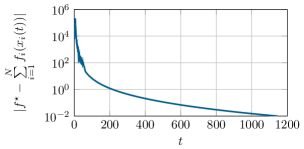
Figure 1: Evolution of the cost error, in logarithmic scale.

In Figure 2 we show the violation of the coupling constraint at each iteration $t$. It is interesting to notice that the violation asymptotically goes to a nonpositive value.

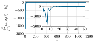
Figure 2: Primal violation evolution of $x_{i}(t)$, $i\in\{1,\ldots,N\}$.

In Figure 3 we show the behavior of $\rho_{i}(t)$, $i\in\{1,\ldots,N\}$, which become zero after some initial iterations, as highlighted in the zoom. This behavior reveals that primal local problems at those iterations would be unfeasible if the relaxation were not present. Thus, the “non-relaxed approach” discussed in Section 3 would not work for this particular numerical example, showing the strength of our relaxed approach.

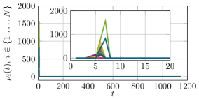
Figure 3: Evolution of $\rho_{i}(t)$, $i\in\{1,\ldots,N\}$.

6 Conclusions

In this paper we have proposed a novel distributed method to solve convex optimization problems with separable cost function and coupling constraints. While the algorithm has a very simple structure (a local minimization and a linear update) its derivation involves a relaxation approach and a deep tour into duality theory. After a constructive derivation of the algorithm, we have proven its convergence. Simulations have corroborated the theoretical results and shown how a first tentative approach, without the relaxation, would not guarantee convergence a priori.

References

• Bertsekas (2009) Bertsekas, D.P. (2009). Min common/max crossing duality: A geometric view of conjugacy in convex optimization. Lab. for Information and Decision Systems, MIT, Tech. Report.
• Bertsekas et al. (2003) Bertsekas, D.P., Nedić, A., and Ozdaglar, A.E. (2003). Convex analysis and optimization. Athena Scientific.
• Bertsekas and Tsitsiklis (1989) Bertsekas, D.P. and Tsitsiklis, J.N. (1989). Parallel and distributed computation: numerical methods, volume 23. Prentice hall Englewood Cliffs, NJ.
• Bürger et al. (2013) Bürger, M., Notarstefano, G., and Allgöwer, F. (2013). From non-cooperative to cooperative distributed MPC: A simplicial approximation perspective. In European Control Conference, 2795–2800. Zurich (Switzerland).
• Bürger et al. (2014) Bürger, M., Notarstefano, G., and Allgöwer, F. (2014). A polyhedral approximation framework for convex and robust distributed optimization. IEEE Trans. on Automatic Control, 59(2), 384–395.
• Chang (2016) Chang, T.H. (2016). A proximal dual consensus ADMM method for multi-agent constrained optimization. IEEE Trans. on Signal Processing, 64(14), 3719–3734.
• Chang et al. (2014) Chang, T.H., Nedić, A., and Scaglione, A. (2014). Distributed constrained optimization by consensus-based primal-dual perturbation method. IEEE Trans. on Automatic Control, 59(6), 1524–1538.
• Falsone et al. (2016) Falsone, A., Margellos, K., Garatti, S., and Prandini, M. (2016). Dual decomposition and proximal minimization for multi-agent distributed optimization with coupling constraints. arXiv preprint arXiv:1607.00600.
• Mateos-Núñez and Cortés (2015) Mateos-Núñez, D. and Cortés, J. (2015). Distributed subgradient methods for saddle-point problems. In IEEE 54th Conference on Decision and Control (CDC).
• Notarnicola et al. (2016) Notarnicola, I., Franceschelli, M., and Notarstefano, G. (2016). A duality-based approach for distributed min-max optimization with application to demand side management. In IEEE 55th Conference on Decision and Control (CDC), 1877–1882.
• Simonetto and Jamali-Rad (2016) Simonetto, A. and Jamali-Rad, H. (2016). Primal recovery from consensus-based dual decomposition for distributed convex optimization. Journal of Optimization Theory and Applications, 168(1), 172–197.
• Tran-Dinh et al. (2016) Tran-Dinh, Q., Necoara, I., and Diehl, M. (2016). Fast inexact decomposition algorithms for large-scale separable convex optimization. Optimization, 65(2), 325–356.