Ion-ion dynamic structure factor, acoustic modes and equation of state of two-temperature warm dense aluminum

Abstract

The ion-ion dynamical structure factor and the equation of state of warm dense aluminum in a two-temperature quasi-equilibrium state, with the electron temperature higher than the ion temperature, are investigated using molecular-dynamics simulations based on ion-ion pair potentials constructed from a neutral pseudoatom model. Such pair potentials based on density functional theory are parameter-free and depend directly on the electron temperature and indirectly on the ion temperature, enabling efficient computation of two-temperature properties. Comparison with ab initio simulations and with other average-atom calculations for equilibrium aluminum shows good agreement, justifying a study of quasi-equilibrium situations. Analyzing the van Hove function, we find that ion-ion correlations vanish in a time significantly smaller than the electron-ion relaxation time so that dynamical properties have a physical meaning for the quasi-equilibrium state. A significant increase in the speed of sound is predicted from the modification of the dispersion relation of the ion acoustic mode as the electron temperature is increased. The two-temperature equation of state including the free energy, internal energy and pressure is also presented.

I Introduction

The challenge of modeling warm dense matter (WDM) — a system of strongly-coupled classical ions and partially degenerate electrons at high temperature and high density — is central to understanding many physical systems such as the interior of giant planets Guillot (1999), laser machining and ablation Lorazo et al. (2003), and inertial-confinement fusion Atzeni and Meyer-ter Vehn (2004). In WDM, neither the kinetic energy nor the potential energy can be treated as a perturbation. Hence the usual theoretical techniques of classical plasma physics or solid-state physics become inapplicable. In the laboratory, WDM can be created through the interaction of high-energy short-pulse lasers with simple metals such as aluminum Fletcher et al. (2015); Ma et al. (2013) and beryllium Lee et al. (2009), with densities $\rho$ several times the room density $\rho_{0}$ and temperatures of the order of 1 eV. The importance of treating these systems as two-temperature WDM systems rather than equilibrium systems has not always been appreciated in analyzing the experimental results Dharma-wardana (2016a); Harbour et al. (2016).

The ion-ion dynamic structure factor (DSF) $S(\mathbf{k},\omega)$ is a key quantity for understanding the WDM regime. For instance, it contains information on the longitudinal waves propagating in the system. The DSF can be measured by neutron scattering and indirectly via X-ray Thomson scattering (XRTS) Glenzer and Redmer (2009). The Chihara decomposition Chihara (1987) has been applied to describe the XRTS signal by partitioning the total electron-electron DSF $S_{ee}(\mathbf{k},\omega)$ in the following form :

$$S_{ee}(\mathbf{k},\omega)=S_{ee}^{0}(\mathbf{k},\omega)+N(\mathbf{k})S_{ii}(\mathbf{k},\omega)+S_{ee}^{fb}(\mathbf{k},\omega).$$ (1)

Here $S_{ee}^{0}$ is the free electron-electron DSF, $S_{ee}^{fb}$ is the contribution from transitions between bound and free electrons, $N(\mathbf{k})=n_{b}(\mathbf{k})+n_{f}(\mathbf{k})$ is the total electron form factor split into a bound part $n_{b}$ and a free part $n_{f}$, and $S_{ii}$ is the ion-ion DSF. Using this decomposition, simulations combining standard density functional theory (DFT) with molecular dynamics (MD) simulations have been used Fletcher et al. (2015); Ma et al. (2013); Rüter and Redmer (2014); Clérouin et al. (2015) to extract properties of WDM systems such as the free electron density per ion $n_{e}$ (i.e., $\bar{Z}$), the ion density $\rho$, the electron temperature $T_{e}$ and the ion temperature $T_{i}$. Since these simulations are computationally expensive, the use of a simpler approach such as the neutral pseudoatom (NPA) model is appropriate. The NPA is well adapted to extract the ion part of the XRTS signals Harbour et al. (2016) and will be the principal method used in this work, where we show that the NPA also has the needed accuracy. The XRTS spectrum can be computed in the NPA, and also by other means without using the Chihara decomposition Vorberger and Gericke (2015); Baczewski et al. (2016) but its discussion is not needed for this work.

However, the separation between ion acoustic modes $\Delta\omega=2\hbar\omega_{p}$, with $\omega_{p}$ the ion-plasma frequency, is of the order of 1 meV, significantly lower than the bandwidth of any X-ray probe laser used experimentally at the moment. Thus, the ion-ion DSF is usually approximated by its static form $S(k,\omega)=S(k)\delta(\omega)$ in describing the XRTS signal. Nevertheless, the ion-ion DSF contains important information about the ion transport properties linked to electron-ion equilibration, formation of coupled modes, interaction with projectiles, etc., which makes it a key quantity for fully understanding the WDM regime. With X-ray laser sources being improved, the ion-ion DSF should become available from future experiments, motivating its calculation for both equilibrium and quasi-equilibrium situations.

Furthermore, in the limit of small wavevectors, $k\rightarrow 0$, the ion-ion DSF can be described in a hydrodynamic framework Hansen and McDonald (2006) (see below), providing important physical quantities such as the adiabatic velocity of sound, the ion acoustic dispersion relation, the thermal diffusivity and the sound attenuation coefficient. In addition, in the case of simple metals commonly probed in most XRTS experiments, the laser interacts mainly with the free-electron subsystem, creating a non-equilibrium system where the electron temperature $T_{e}$ is higher than the initially cold ions at temperature $T_{i}$. It has been shown that, when the shock wave resulting from the laser pulse has propagated through the sample and reaches the probing location, the system might still be in a two-temperature ($2T$) state Harbour et al. (2016); Dharma-wardana (2016a). Since the ion-ion interactions in simple metals are related to the screening of the free-electron subsystem, the quasi-equilibrium properties of the total system with $T_{e}\neq T_{i}$ differ significantly from the equilibrium ones. The hardening of the phonon spectra in ultra-fast matter Harbour et al. (2015, 2017); Recoules et al. (2006), where $T_{e}$ is about 1 eV while $T_{i}$ remains at room temperature $T_{r}$, is an example of how the ion dynamics can be affected drastically in such conditions. Transport properties of Al in the two-temperature regime, such as self-diffusion and shear viscosity, are also significantly modified Hou et al. (2017).

The ion-ion DSFs for WDM have been calculated mainly using DFT coupled to classical molecular dynamics (MD) Rüter and Redmer (2014) simulations. Since DSF calculations require a large number of particles and long simulation times, DFT-MD calculations are computationally very intensive. In addition, the finite-$T$ treatment of the electronic subsystem in DFT requires the solution of the Kohn-Sham equations for many electronic bands to take thermal excitations according to the Fermi-Dirac distribution into account. Orbital-free (OF) DFT simulations do not require electronic wave functions, but require a Hohenberg-Kohn kinetic-energy functional as well as a finite-$T$ generalization thereof. Such procedures are less accurate than the Kohn-Sham method, but make the simulations practical White et al. (2013). The full DFT-MD simulations when feasible can be used to benchmark simpler methods like the NPA or OF approaches which are easily applied over a wider range of temperatures and densities.

In the present work, we compute the ion-ion DSF using classical MD simulations based on pair potentials (PP) constructed from the NPA model, which is a fully based on DFT. The NPA approach has already been used to predict the DSF of strongly-coupled hydrogen plasmas Nardin et al. (1988) and provides the sound velocity, the thermal diffusivity, the specific-heat ratio, and the viscosity. The NPA-PPs are free of ad hoc parameters and are accurate to within a few meV as established by the prediction of accurate experimental phonon spectra for simple WDM solids Harbour et al. (2015, 2017). The NPA-PP-predictions for static structure factors (SSF) obtained using the modified-hyper-netted-chain (MHNC) approximation are in agreement with DFT-MD simulations for WDM systems (typical examples are Be and Al Harbour et al. (2016); for a review of the NPA, see Ref. Dharmawardana, 2015).

Furthermore, in the quasi-equilibrium case, i.e. when $T_{e}$ is different from $T_{i}$, the extension of the NPA approach to two-temperature ($2T$) situations has enabled the construction of $2T$-PPs which reproduce ab initio calculations of quasi-equilibrium phonon spectra Harbour et al. (2017), quasi-equilibrium XRTS signals Harbour et al. (2016), and frequency-dependent $2T$ plasmon profiles Dharma-wardana (2016a) and conductivities of ultra-fast matter Dharma-wardana et al. (2017). The objective of the present study is to determine the DSF $S(k,\omega,T_{e},T_{i})$ in the $2T$ regime. In addition, we evaluate the $2T$ equation of state (EOS). All calculations are carried out for aluminum at the ‘room temperature’ density of $\rho_{0}$ = 2.7 g/cm³ with the ion temperature fixed at $T_{i}=1$ eV while the electron temperature $T_{e}$ is varied between 1 and 10 eV.

II Methods

II.1 Neutral-pseudoatom model

The NPA model Dagens (1972, 1975); Perrot (1993) is a rigorous all-electron DFT average-atom approach where the ion distribution is also treated in DFT Dharma-wardana and Perrot (1982). Given the mean free-electron density $n$ and electron temperature $T_{e}$, it determines the total electron density around a single Kohn-Sham ion constructed from a nucleus of charge $Z_{n}$ embedded in the plasma environment of mean density $\rho$. A classical Kohn-Sham equation for the ions determines the one-body ion distribution $\rho(r)=\rho g_{ii}(r)$, where $g_{ii}(r)$ is the ion pair distribution function (PDF), abbreviated to $g(r)$. The classical Kohn-Sham equation for the ions is identified as a type of hyper-netted chain (HNC) integral equation bringing in ion-ion correlations beyond the mean-field approximation. The Kohn-Sham-Mermin solutions are obtained in the local-density approximation using a finite-$T_{e}$ free-energy exchange-correlation (XC) functional $F_{xc}[n,T_{e}]$ Perrot and Dharma-wardana (2000). The available finite-$T$ XC-functionals, fitted to quantum Monte-Carlo results or to the classical-map HNC results (used here), yield numerically equivalent results in WDM applications Dharma-wardana (2016b).

In order to simulate the effect of the ion-density $\rho(r)$ on the electronic states, a uniform positive neutralizing background with a spherical cavity of radius $r_{\rm ws}$, with the nucleus at the origin, is used. Here, $r_{\rm ws}=[3/(4\pi\rho)]^{1/3}$ is the Wigner-Seitz radius of the ion. This lowest-order model for $\rho(r)=\rho g(r)$ is sufficient for calculating the Kohn-Sham energy levels of “simple metal” ions immersed in a warm dense electron fluid, as has been discussed in a recent review Dharmawardana (2015). The adjustment of the ion distribution to the electron distribution is accomplished by the optimization of a single parameter, viz. $r_{\rm ws}$, subject to the finite-$T$ Friedel sum rule Dharma-wardana and Perrot (1982). Although, strictly speaking, an electron-ion exchange-correlation functional is also needed Perrot et al. (1990), it is neglected here.

An advantage of the NPA model is that it directly provides single-ion properties such as the mean ionization $\bar{Z}$ and the electron density around the nucleus $n(r)=n_{b}(r)+n_{f}(r)$, with $n_{b}$ and $n_{f}$ the bound and free electron densities, respectively. In simple metals, $n_{b}$ is found to be localized within a radius much smaller than $r_{\rm ws}$, such that $n_{b}(r\to r_{\rm ws})=0$, which enables a clear definition of the mean ionization $\bar{Z}=n-n_{b}$. Note however, that the free-electron distribution is not restricted to the WS-sphere, as is done in many average-atom (AA) models, as reviewed by, e.g., Murillo et al. Murillo et al. (2013).

The free electrons occupy the whole space, modeled by a large correlation sphere of radius $R_{c}$ of about 10 WS radii, usually sufficient to include all particle correlations associated with the central nucleus. Unlike in AA models, the mean number of free electrons per ion, viz. $\bar{Z}$, is an unambiguously defined quantity subject to the Friedel sum rule, and experimentally measurable using XRTS Glenzer and Redmer (2009), static conductivities, Langmuir probes, etc. The interaction among ions of charge $\bar{Z}$ is screened by the free electron subsystem which is assumed to respond linearly to the electron-ion pseudopotential

$$U_{ei}(k,T_{e})=n_{f}(k)/\chi(k,T_{e}).$$ (2)

Since $n_{f}(k)$ is determined by the Kohn-Sham calculation which goes beyond the linear response to $\bar{Z}/r$, the above pseudopotential actually includes all the non-linear DFT effects within a linearized setting. The limits of validity of this procedure are discussed in Ref. Dharma-wardana (2012).

With $n_{f}(k)$ at hand, $U_{ei}$ is constructed using the finite-$T$ interacting electron response function

$$\chi(k,T_{e})=\frac{\chi_{0}(k,T_{e})}{1-V(k)[1-G(k,T_{e})]\chi_{0}(k,T_{e})}$$ (3)

with $\chi_{0}$ the finite-$T$ non-interacting Lindhard function, $V(k)=4\pi/k^{2}$ the bare Coulomb interaction, and $G$ a finite-$T$ local-field correction Harbour et al. (2015) which depends directly on $F_{xc}$. Finally, the screened ion-ion pair interaction is given by

$$V_{ii}(k,T_{e})=\bar{Z}^{2}V(k)+|U_{ei}(k,T_{e})|^{2}\chi(k,T_{e});$$ (4)

This pair potential is the NPA input to the classical MD calculations.

It should be noted that the NPA uses a pair-potential for the ions and does not attempt to include multi-ion potentials, as is customary in effective medium (EM) approaches that have been successfully used for metals and semiconductors, especially at ambient temperature and compression. The EM method is at best a non-selfconsistent DFT approach Depristo (2011) which includes two-body, three-body and other multi-ion effects. It is often further extended by fitting to empirical and calculational databases. However, recent attempts to use such models for, e.g., WDM carbon, have not been very successful Kraus et al. (2013). The NPA approach exploits the fact that the grand potential $\Omega[n,\rho]$ is a functional of both the one-electron distribution $n(r)$ and the one-ion distribution $\rho(r)$. Hence a single-ion description (which allows a pair potential) is the only rigorously necessary information for a full DFT description of the system. In practice, pair potentials are sufficient if linear-response pseudopotentials could be constructed, as in Eq. 2. However, this approach now needs, not only an XC-functional for the electrons, but also a correlation functional for the classical ions. These are constructed via classical integral equations, or automatically via MD simulations. Detailed discussions of these issues and the NPA method may be found in Refs. Dharma-wardana (1993); Dharmawardana (2015). In this context, we remark that standard implementations of DFT-MD in codes like ABINIT and VASP Gonze et al. (2009); Kresse and Furthmüller (1996) use only the one-electron density-functional property, and not the one-ion density functional, as it chooses to implement a full $N$-ion Kohn-Sham simulation with $N$ typically of the order of 100 or more.

Furthermore, the multi-center nature of the simulations implies a highly non-uniform electron density requiring sophisticated gradient-corrected XC-functionals. In contrast, the NPA uses a relatively smooth single-center electron distribution for which the local-density approximation (LDA) is found to work very well, even for sensitive properties like the electrical conductivity Dharma-wardana et al. (2017) and plasmon spectral line shapes Dharma-wardana (2016a). The LDA form of the finite-$T$ XC-functional of Perrot and Dharma-wardana Perrot and Dharma-wardana (2000) is used in this study.

II.2 Dynamic Structure Factor

The ion-ion spatial and temporal correlations are determined from the van Hove function

$$G(\mathbf{r},t) =\frac{\langle\rho(\mathbf{r},t)\rho(\mathbf{0},0)\rangle}{\rho}$$ (5)

$$=\frac{1}{N}\left\langle\sum_{i=1}^{N}\sum_{j=1}^{N}\delta[\mathbf{r}-\mathbf{r}_{j}(0)-\mathbf{r}_{i}(t)]\right\rangle$$

with $\langle\cdot\cdot\cdot\rangle$ the ensemble and time average (over many different time origins) calculated from classical MD simulations of a $N$-particle system, $\rho$ the mean ion density, and $\mathbf{r}_{i}(t)$ the position of the $i$-th ion at time $t$. The ion-ion DSF

$$S(\mathbf{k},\omega)=\frac{1}{2\pi}\int_{-\infty}^{\infty}F(\mathbf{k},t)\ e^{i\omega t}dt$$ (6)

is the time Fourier transform of the intermediate scattering function $F(\mathbf{k},t)$, which is itself the spatial Fourier transform of the Van Hove function

$$F(\mathbf{k},t)=\int G(\mathbf{r},t)e^{-i\mathbf{k}\cdot\mathbf{r}}d\mathbf{r}.$$ (7)

While $G(\mathbf{r},t)$ contains much information relevant to $2T$ situations, $F(\mathbf{k},t)$ is also directly accessible in MD simulations via the relation

$$F(\mathbf{k},t)=\frac{1}{N}\langle\rho_{\mathbf{k}}(t)\rho_{-\mathbf{k}}(0)\ \rangle$$ (8)

where

$$\rho_{\mathbf{k}}(t)=\sum_{i}^{N}e^{i\mathbf{k}\cdot\mathbf{r}_{i}(t)},$$ (9)

thus avoiding the calculation of the spatial Fourier transform which can add spurious high-frequency oscillations to $F(\mathbf{k},t)$ due to the finite size of the MD simulation cell. Under WDM conditions, the averaged system properties are those of an isotropic fluid; thus important structural quantities are spherically-symmetric in real space, $|\mathbf{r}|=r$, and in reciprocal space, $|\mathbf{k}|=k$.

In the hydrodynamic limit, $k\to 0$, the DSF takes the so-called ‘three-peak’ form

$$S(k,\omega)=\frac{S(k)}{2\pi}\left[\left(\frac{\gamma-1}{\gamma}\right)\frac{2D_{T}k^{2}}{\omega^{2}+(D_{T}k^{2})^{2}}\right.$$ (10)

$$+\left.\frac{1}{\gamma}\left(\frac{\Gamma k^{2}}{(\omega-c_{s}k)^{2}+(\Gamma k^{2})^{2}}+\frac{\Gamma k^{2}}{(\omega+c_{s}k)^{2}+(\Gamma k^{2})^{2}}\right)\right]$$

with $D_{T}$ the thermal diffusivity, $\Gamma$ the sound attenuation coefficient, $\gamma=c_{P}/c_{V}$ the ratio of the constant pressure to the constant volume specific heats, $c_{p}$ and $c_{V}$, and $c_{s}$ adiabatic speed of sound. The second and third terms of Eq. 10 are the Brillouin peaks whose positions provide the acoustic dispersion relation $\omega_{s}(k)$, which is linear at small $k$, $\omega_{s}(k\to 0)=c_{s}k$, and is measurable experimentally. In addition, it is also possible to compute $c_{s}$ from the SSF $S(k)$ using the compressibility $\kappa$ sum rule $S(0)=\rho\kappa T_{i}$ which leads to $c_{s}=\sqrt{T_{i}/S(0)}$. Once the PP is constructed, the SSF can be easily calculated via the MHNC procedure, independent of MD simulations.

II.3 Equation of State

The total free energy per atom in the NPA model is given by

$$F=F_{e}^{0}(T_{e})+F_{\text{emb}}(T_{e})+F_{ii}(T_{i},T_{e})+F_{i}^{0}(T_{i}),$$ (11)

with contributions $F_{e}^{0}$ from the interacting homogeneous electron gas, $F_{\text{emb}}$ from the embedding of the pseudoatom into the uniform system, $F_{ii}$ from the interacting ion-ion system, and $F_{i}^{0}$ from the ideal ion gas. A more detailed description of each term of the NPA free energy is given in Refs. Perrot (1993); Perrot and Dharma-wardana (1995). For the equilibrium system, the pressure is obtained via the density derivative of the free energy while the internal energy is obtained by taking the temperature derivative:

$$P=n^{2}\frac{\partial F}{\partial n},\qquad E=\frac{\partial(\beta F)}{\partial\beta}$$ (12)

with $\beta=1/T$. For quasi-equilibrium systems, the internal energy must be computed taking into account the temperature derivative of each contribution in Eq.11. Note that the term $F_{ii}$ depends on both $T_{i}$ and $T_{e}$. Thus, the total derivative of the $2T$ internal energy reads

$$E(T_{e},T_{i})\equiv\frac{\partial(\mathbf{\beta}F)}{\partial\mathbf{\beta}}=F+\left.\frac{\partial F}{\partial\beta_{e}}\right|_{T_{i}}+\left.\frac{\partial F}{\partial\beta_{i}}\right|_{T_{e}}$$ (13)

which recovers the correct equilibrium internal energy when $T_{i}=T_{e}$.

III Results

All DSF have been calculated from MD simulations using the NPA pair potentials. The initial configuration was a face-centered cubic crystal containing 5324 particles arranged in a cubic simulation cell. This corresponds approximately to a linear dimension of 17 to 18 Wigner-Seitz radii, i.e., significantly larger than typical ion-ion correlations seen in the ion-ion pair distribution of aluminum even at its melting point. Simulations were carried out over 0.5 ns with a timestep of 0.5 fs. The first 50,000 steps have not been used as they pertain to the initial equilibration period. From the remaining simulation, configurations have been extracted every 1 fs for the calculation of $G(r,t)$ and $F(k,t)$ which have been calculated up to 3000 fs. The ion temperature was kept constant throughout the simulation using a Nosé-Hoover thermostat. The electron temperature no longer appears in the dynamics, so no electron thermostat is needed; $T_{e}$ only intervenes in the construction of the NPA pair potential, which is the essential ‘quantum input’ to the classical MD simulation.

In the range of $T_{e}$ studied in this work, i.e. from 1 to 10 eV, the mean ionization calculated from the NPA model remained essentially unchanged from the room temperature value of $\bar{Z}=3.0000$ to 3.0163 for the normal density of 2.7 g/cm³. Given a Fermi energy (i.e, approximately the chemical potential) of $\sim$ 12 eV, no significant change in $\bar{Z}$ is in fact expected. There is even less of a change at the higher density of 5.2 g/cm³ used by Rüter et al Rüter and Redmer (2014), as the Fermi energy is correspondingly higher. The value of $\bar{Z}$ for Al begins to increase only from about 20 eV, and the consistency of the NPA evaluated $\bar{Z}$ even at higher temperatures is shown from its successful prediction of electrical conductivities of aluminum under a variety of WDM conditions Dharma-wardana et al. (2017); Benage et al. (1999).

III.1 Static properties

We first review the results for several key static properties, viz.  pair-potentials, PDFs, and structure factors.

III.1.1 Pair-potentials

The easily computed NPA ion-ion pair-potentials described by Eq. 4 are the starting point of our study of the aluminum DSF, using classical molecular dynamics with the NPA-PPs as the input. Hence, in Fig. 1 we show typical Al-Al pair potentials that are relevant to our study. These pair potentials are the simplest that can be constructed from the NPA density, while the NPA calculation provides enough data to construct more complex non-local pseudopotentials, or potentials designed to recover phase shifts, etc. However, such elaborations need to be invoked only if such potentials are really required. We have found that this elementary approach works well for simple metallic fluids in regimes of compressions of 0.5 to about 2.5, and from low temperatures (e.g., melting point) to higher temperatures (where the model works better). In the present study (aluminum at 2.7 g/cm³, and 5.2 g/cm³, at $T$=1 eV and 5.4 eV, the model is eminently applicable, as we show by comparisons with more microscopic simulations for the PDFs and other properties given below.

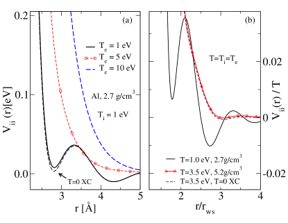
Figure 1: (color online) (a) Ion-ion pair potentials constructed from the NPA model at electron temperatures of $T_{e}=$ 1, 5, and 10 eV, while the ion temperature is held at $T_{i}$ = 1 eV. (b) The $T_{i}=T_{e}=1$ eV potential for the ‘room temperature’ Al density 2.7 g/cm³, as well the pair potential at 5.2 g/cm³ and T=3.5 eV relevant to the work of Rüter Rütter and Redmer Rüter and Redmer (2014). Note that in panel (b) we have plotted the potentials in terms of physically relevant variables $r/r_{\rm ws}$ and $V_{ii}(r)/T$, where the nominal WS radii $r_{\rm ws}$ are 2.991 a.u. and 2.404 a.u, respectively.

Panels (a), (b) show the crucial role played by the Friedel oscillations in the potentials. These are evident in the potential at $T_{e}=1$ eV and more weakly in the 3.5 eV potential. At high $T_{e}$, they are damped out and the potentials become more Yukawa-like. The NPA model faithfully reproduces these potentials to good accuracy, whereas many commonly-used average-atom models do not. The location of these oscillations, as well as packing effects in the fluid, are controlled by $r_{\rm ws}$. Hence the plot using $r/r_{\rm ws}$ as the $x$-coordinate brings potentials at different densities to a comparable footing. We also show the pair-potential at 5.2 g/cm³ and $T$=3.5 eV calculated using the $T$=0 XC-functional that is customarily implemented in DFT-MD simulations, showing a small and probably negligible difference. However, it should be always remembered that standard DFT-MD simulations can be used to benchmark other calculations only when the $T=0$ XC approximation holds.

III.1.2 Pair Distribution Function

The NPA-PPs are known to closely reproduce the ion-ion PDF $g(r)$ and the corresponding static structure factor $S(k)$ for most systems studied so far, for compressions of 0.5 to about 2.5. Some examples are :
(i) Al (a) at normal density $\rho=2.7$g/cm³ and at the melting point, and (b) at an expanded density $\rho=2.0$ g/cm³ with $T=$ 1,000K and 5,000K Dharma-wardana (2006),
(ii) Li at $T=2000$ K and $\rho=0.85$ g/cm³Harbour et al. (2017),
(iii) Be at densities of $\rho=1.85$ g/cm³ and $\rho=5.53$ g/cm³ for various two-temperature situations Harbour et al. (2016), and
(iv) C, Si and Ge in the WDM state Dharma-wardana (2016c); Dharma-wardana and Perrot (1990). Here, because of the high electron density ($\bar{Z}=4$) the NPA model works even at 12 g/cm³, i.e, close to six times the graphite density.

While liquid metal PDFs can be obtained from MD simulations using multi-center potentials such as those available from EM theory Depristo (2011), embedded-atom model (EAM) approaches Waseda (1980), or bond-order potentials Ghiringhelli et al. (2005), they have not been applied in an intensive way to the WDM regime. The effect of $T_{e}$ on the ion-ion interaction is not included except in limited cases Khakshouri et al. (2008). Kraus et al. Kraus et al. (2013) examined the use of multi-ion bond-order potentials for WDM carbon but found them to be unsuitable and extremely difficult to formulate for finite-$T$ usage. In contrast, the NPA-PPs are simple to compute and are at finite-$T$ from the outset. Here we show that the PDFs obtained from them agree closely with those from DFT-MD for the systems studied here.

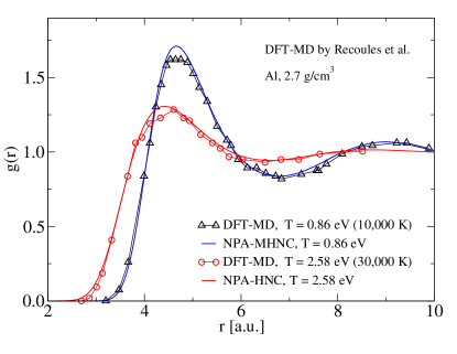
Figure 2: (color online) A comparison of the $g(r)$ from the NPA-MD and from DFT-MD simulations (Recoules et al. Recoules et al. (2015) for Al at the normal density $\rho_{0}$ and at 10,000K and 30,000K. No bridge terms are needed at the higher $T$ case, where HNC and MHNC become equivalent).

In Fig.2 NPA PDFs for aluminum at the ‘normal’ density $\rho_{0}$ are compared with DFT-MD simulations from Recoules et al at 10,000 K and 30,000 K Recoules et al. (2015). The agreement is relatively good. The slight disagreement ($\sim$ 4%) noted near the main peak is a common feature in this type of comparison, arising from statistical noise in MD simulations with, say $N\sim$ 100 atoms. Here one may expect fluctuations of $\sim 1/\surd{N}$. In reality, the need to take an ensemble average of every quantity in DFT-MD simulations adds to the labour and cost. In Fig.3, we compare the PDF for Al obtained from the NPA pair potentials with that from Kohn-Sham DFT-MD simulations for two cases. The first case (panel (a) in Fig.3) is for the room temperature density $\rho=2.7$ g/cm³ at a temperature $T=1$ eV, which gives one of the equilibrium WDMs used in this study. The second case (panel (b) in Fig.3) is for the compressed density $\rho=5.4$ g/cm³ at a temperature $T=3$ eV which is close to the conditions used by Rüter and Redmer Rüter and Redmer (2014) in their DFT-MD calculation of the aluminum DSF. The latter is used in section III.2 to compare with our NPA-MD DSF. Our DFT-MD simulations were done with the ABINIT package using a cell of 108 atoms with a norm-conserving pseudopotential and the $T=0$ Perdew-Burke-Ernzerhof exchange and correlation functional within the generalized gradient approximation. In this case, the position of the first maxima in $g(r)$ are within 1% of each other for the first case (a) and within 2% at for the second case (b). The height of the first peak differs by about 3% in both cases showing the good aggreement between DFT-MD and NPA-MD simulations. The use of pair potentials to perform classical MD simulations requires a considerably shorter amount of time illustrating the advantage of employing the NPA model.

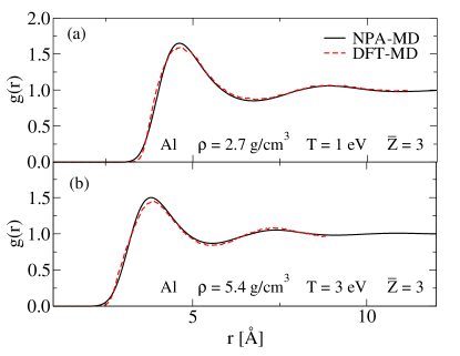
Figure 3: (color online) Comparison of the $g(r)$ from the NPA-MD and from DFT-MD simulations for two Al WDM states: (a) $\rho$ at the room temperature density of 2.7 g/cm³, $T=1$ eV, and (b) $\rho=5.4$ g/cm³, $T=3$ eV.

III.1.3 Static Structure Factor

As indicated in Sec.II.2, $c_{s}$ can also be calculated from the SSF using the compressibility sum rule. In Fig. 4, we compare the $S(k)$ computed from HNC, MHNC and MD simulations all using the same pair potential. We note that the MHNC SSF and the MD SSF agree very well, while the HNC predicts a slightly lower maximum and a slightly different $k=0$ limit. This suggests that the differences may be due to the use of a hard-sphere model within the Lado-Foiles-Ashcroft criterion for modeling the bridge function Lado et al. (1983). In principle, more accurate bridge functions can be extracted from MD simulations.

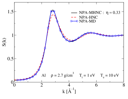
Figure 4: (color online) $S(k)$ computed from MHNC (continuous line), HNC (red dashed line) and MD (blue circles and blue line) simulations at $T_{i}$=1 eV and $T_{e}$=10 eV.

III.2 Dynamical properties

III.2.1 Dynamical Structure Factor: Equilibrium system

In this section, the DSF for equilibrium Al, $T_{i}=T_{e}$, obtained from the NPA-PP, is compared with other DSF calculations. First we consider the results of Rüter and Redmer Rüter and Redmer (2014) who used Kohn-Sham DFT-MD to study Al at a density of $\rho=5.2$ g/cm³ (compression $\sim 2$) and $T=3.5$ eV, i.e., $T/E_{f}\simeq 0.19$. In Fig.5, the NPA-MD DSF is compared with the DFT-MD DSF for $k=0.42\ \text{\AA}^{-1}$ and $k=0.69\ \text{\AA}^{-1}$. The position and profile of the Brillouin peak obtained from the NPA-MD agree closely with results from DFT-MD. Furthermore, the speed of sound obtained by Rüter and Redmer, $c_{s}=10.38$ km/s, and the NPA value of $c_{s}=10.62$ km/s are within 2.3% of each other. In this case, the NPA calculation satisfies the $f$-sum rule to within 96$\%$ over the range of $k$ studied.

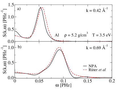
Figure 5: A comparison of the dynamic structure factors obtained from NPA-MD (this work) and DFT-MD Rüter and Redmer (2014) at two different wavevectors. In NPA-MD, the pair potential (Eq. 4) is the input to simulation.

Since a full Kohn-Sham DFT-MD calculation as given by Rüter et al. Rüter and Redmer (2014) for the the DSF is extremely costly, simpler approaches based on average-atom models as well as orbital-free methods have been used to compute the ion-ion DSF. Here we compare the results from the NPA-MD with corresponding results from the pseudoatom model of Starrett and Saumon Starrett and Saumon (2015)(PA-SS), and with OF-DFT-MD simulations, for Al at the density $\rho_{0}$ and $T$ = 5 eV. A comparison of our NPA-MD calculations with the OF-DFT-MD simulations of White et al. White et al. (2013) and those of Gill et al. Gill et al. (2015), using the PA-SS and MD, is presented in Fig. 6 for wavevectors $k=0.45\ \text{\AA}^{-1}$ and 0.96 $\text{\AA}^{-1}$. White et al. used 108 ions in a cubic supercell in an OF-DFT approach. Gill et al. presented an OF model calculation with a classical simulation with 10,000 ions, and also a Kohn-Sham (KS) approach within their PA-SS model. Since our NPA model uses the KS procedure, only the KS-PA-SS results are compared in Fig. 6.

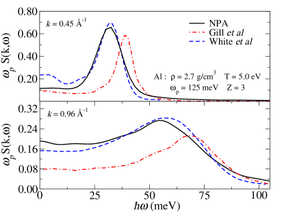
Figure 6: (color online) The equilibrium DSF of Al at density $\rho=\rho_{0}$ and $T$ = 5 eV, for wavevector $k=0.45\ \text{\AA}^{-1}$ (upper panel) and 0.96 $\text{\AA}^{-1}$ (lower panel): NPA (black continuous line), PA-SS Gill et al. (2015) (red dot-dashed line) and OF-DFT-MD White et al. (2013) (blue dashed line).

The positions of the Brillouin peak for $k$ = 0.45 $\text{\AA}^{-1}$ coincide for OF-DFT-MD and NPA-MD, and the peak heights differ by $\sim$4%. The adiabatic speed of sound $c_{s}=\omega_{s}/k$ was obtained by a linear fit to the dispersion relation $\omega_{s}(k)$ for small value of $k$. The OF-DFT-MD predicts an adiabatic speed of sound of 10.4 km/s, very close to the NPA-MD value of 10.2 km/s whereas the PA-SS-MD predicts a higher value of 12.7 km/s. Once again, we ensured that the NPA calculation satisfies the $f$-sum rule to within 97$\%$ over the range of $k$ studied. The good agreement between the equilibrium DSF calculated via the NPA-MD and OF-DFT-MD mutually confirm the extent of validity of these methods and of the NPA-MD approach. We already noted the good agreement with the fully microscopic calculations of Rüter et al Rüter and Redmer (2014). All these encourage us to apply $2T$-NPA-PP to investigate dynamical properties of quasi-equilibrium systems where $T_{e}\neq T_{i}$.

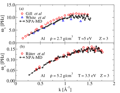
Figure 7: (color online) A comparison of the equilibrium acoustic dispersion relation of Al for (a) density $\rho=\rho_{0}$ and $T$ = 5 eV as in the OF-DFT-MD calculations of White et al White et al. (2013) and as in the PA-SS calculations of Gill et al Gill et al. (2015), and (b) $\rho=5.2$ g/cm³ and $T$ = 3.5 eV as in Rüter et al Rüter and Redmer (2014).

III.2.2 Dynamical Structure Factor: Quasi-equilibrium system

In order to study the ion dynamics in the quasi-equilibrium system with $T_{e}>T_{i}=1$ eV, we employ the ion-ion pair potential $V_{ii}(r,T_{e})$ constructed from the NPA calculation which explicitly depends directly on $T_{e}$. The dependence on $T_{i}$ comes in via the ion density and the ionization state $\bar{Z}$ of the ions, and hence is implicitly included in the NPA calculation. In Fig. 1(a) we present the potentials for the cases $T_{e}=$ 1, 5, and 10 eV. At $T_{e}=1$ eV, the potential exhibits Friedel oscillations with several minima, whereas it becomes purely repulsive at higher temperatures since the Fermi energy at 2.7 g/cm³ is 11.65 eV.

To ensure that the two-temperature DSF of the quasi-equilibrium system is physically relevant, we must verify that all spatial correlations vanish in a time $\tau_{c}$ smaller than the ion-electron relaxation time $\tau_{ei}$, which is of the order of hundreds of picoseconds Dharma-wardana (2001). The Van Hove function has been calculated for the specific case $T_{i}=1$ eV and $T_{e}=10$ eV and its time evolution is presented in Fig. 8. We find that at $\tau_{c}=125$ ps, all spatial correlations have vanished, such that $\tau_{c}<\tau_{ei}$, implying that dynamical properties can be meaningfully calculated for the quasi-equilibrium system.

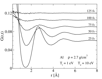
Figure 8: The Van Hove function for different times for the case $T_{i}=1$ eV and $T_{e}=10$ eV. For clarity, each curve is shifted vertically by 0.015 from the previous one while the curve for $t=25$ fs is unshifted.

The $2T$-DSF at $\rho=\rho_{0}$, computed with the NPA-based PP, is presented in Fig. 9 for $T_{i}=1$ eV and $T_{e}=1,5$ and 10 eV and wavevector $k=0.45$ $\text{\AA}^{-1}$. The position of the Brillouin peak shifts to higher $\omega$ as $T_{e}$ increases while the value at $\omega=0$ is drastically lowered. Furthermore, the shape of the peak is narrower for higher $T_{e}$.

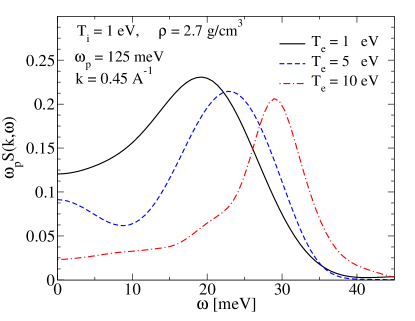
Figure 9: (color online) The quasi-equilibrium DSF of Al at density $\rho_{0}$, $T_{i}$ = 1 eV and $T_{e}=1,5$, $T$= 10 eV, for wavevector $k=0.45\ \text{\AA}^{-1}$.

The dispersion relation $\omega_{s}(k)$ for $T_{e}=1,5$ and $10$ eV can be deduced from the position of the Brillouin peak. It is displayed in Fig. 10.

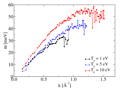
Figure 10: (color online) The two-temperature dispersion relation $\omega_{s}(k)$ calculated from the position of the Brillouin peak for $T_{i}=1$ eV and $T_{e}=$ 1, 5, and 10 eV.

The dispersion relation begins to be noisy and unphysical at different values of wavevector $k$ as $T_{e}$ is increased. Thus the position of the Brillouin peak could be confidently determined only up to $k=$ 0.8, 1.2, and 1.5 $\text{\AA}^{-1}$ for $T_{e}=$ 1, 5, and 10 eV, respectively. Establishing that collective excitations still exist for higher values of $k$ becomes more difficult as the Brillouin peak merges back with the Rayleigh peak at $k=0$. This makes it hard to evaluate the full width at half maximum of the Brillouin peak, ideally needed to establish the survival of longitudinal modes at higher $k$ and higher $T_{e}$. Instead, we decided to include the position of the peak as long as its height is at least 20$\%$ higher than the value at $k=0$. Using the same procedure for each combination of $T_{i}$ and $T_{e}$ enables us to treat them in a comparable manner. Longer MD simulations would yield better results for $\omega_{s}(k)$; however the current results are sufficiently precise to conclude that there exist more ion longitudinal modes at $T_{e}=$ 10 eV than at lower $T_{e}$; this may be due to the lower compressibility of the electron subsystem as well as the ion subsystem with a more repulsive pair potential, as shown in Fig. 1, the ion temperature being identical. These dispersion relations will be used to determine the speed of sound $c_{s}$ as a function of $T_{e}$. Predictions of the speed of sound computed from the DSF, the MHNC-SSF and the HNC-SSF are compared in Fig. 11.

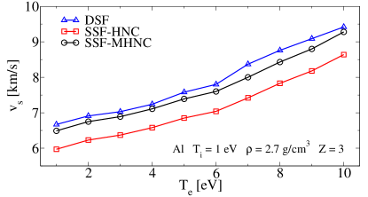
Figure 11: (color online) Comparison of the speed of sound in the $2T$-system calculated from the SSF and from the DSF with $T_{i}=1$ eV.

The speed of sound calculated from the DSF is slightly and systematically higher than the MHNC-SSF value through the entire range of $T_{e}$, with a maximum difference of 4.6$\%$ occurring at $T_{e}=7$ eV; both methods predict a 43$\%$ increase from $T_{e}=1$ to 10 eV. These results also confirm the phenomenon of phonon hardening Recoules et al. (2006). It should be noted that the HNC-SSF value is considerably lower than the value from other methods, illustrating the importance of using a bridge term in the integral equation for the ion distribution at these coupling strengths.

III.3 Quasi-Equation of State

The NPA model allows a rapid calculation of the EOS of Al in equilibrium conditions, which was intensively investigated by Sjostrom et al Sjostrom et al. (2016), but also for $2T$ situations. In Fig. 12 we present a comparison between the equilibrium and the quasi-equilibrium Helmholtz free energy $F$, internal energy $E$, and total pressure $P$. At the highest electronic temperature ($T_{e}=10$ eV) that we have studied, the equilibrium $F$ is lower than that of the quasi-equilibrium system by 2.3$\%$ while the internal energy is higher by 0.25$\%$. The internal energy in both cases has a maximum in the range of $T_{e}=6-7$ eV and has a similar shape. While $F$ and $E$ are only slightly modified in the $2T$ regime, the equilibrium pressure is higher than that obtained at quasi-equilibrium by as much as 56 $\%$ at $T_{e}$=10 eV.

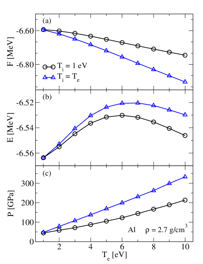
Figure 12: (color online) Comparison between the equilibrium and quasi-equilibrium free energy (a), internal energy (b), and pressure (c) of Al at density $\rho_{0}$. As $T_{i}$ is held fixed at 1 eV for quasi-equilibrium time scales (or longer via a thermostat coupled only to the ions), the ionic lattice does not expand and the density remains fixed.

Even though the changes in the free energy and internal energy are small, such variations could considerably affect EOS-dependent properties such as specific heats, conductivities, energy relaxation rates and other coupling coefficients that enter into more macroscopic WDM simulations. The efficiency and rapidity of computing such $2T$-EOS via the NPA model allows to obtain them on the fly for simulations of shocked or laser-driven systems, for most combinations of $T_{i}$ and $T_{e}$ where a significant density of free electrons is available to make the NPA approach valid, and where no persistent chemical bonds are formed.

IV Conclusion

Taking aluminum as an example, we demonstrated that the NPA pair potentials can be used to compute efficiently and accurately the equilibrium dynamic structure factor via MD simulations, and established that it is in close agreement with DFT-MD results. We explored the two-temperature system and showed that all ion-ion correlations vanish in a time shorter than typical electron-ion relaxation times, validating the concept of a $2T$-dynamic structure factor in this context.

We presented the $2T$-DSF and showed that the Brillouin peak shifts to higher energies as the electron temperature is increased. As a result, the ion acoustic mode dispersion relation is modified and the adiabatic speed of sound $c_{s}$ is increased, in good agreement with its determination via the compressibility sum rule in the small-$k$ limit of the static structure factor. The latter is independently obtained via the modified hyper-netted chain method and using the pair potentials generated via the neutral-pseudoatom method. The increase in the acoustic velocity is also consistent with the phenomenon of ‘phonon hardening’.

The comparison between the equilibrium and quasi-equilibrium EOS shows that the free energy and the internal energy are only weakly modified in the two-temperature system, while the pressure is significantly affected. The efficient calculation of the quasi-equilibrium EOS via the neutral pseudoatom method constitutes a powerful tool for exploring out-of-equilibrium systems via MD simulations.

References

- Guillot (1999) T. Guillot, Science 286, 72 (1999).
- Lorazo et al. (2003) P. Lorazo, L. J. Lewis, and M. Meunier, Phys. Rev. Lett. 91, 225502 (2003).
- Atzeni and Meyer-ter Vehn (2004) S. Atzeni and J. Meyer-ter Vehn, The Physics of Inertial Fusion: Beam-Plasma Interaction, Hydrodynamics, Hot Dense Matter (Clarendon Press, Oxford, 2004).
- Fletcher et al. (2015) L. B. Fletcher, H. J. Lee, T. Döppner, E. Galtier, B. Nagler, P. Heimann, C. Fortmann, S. LePape, T. Ma, M. Millot, A. Pak, D. Turnbull, D. A. Chapman, D. O. Gericke, J. Vorberger, T. White, G. Gregori, M. Wei, B. Barbrel, R. W. Falcone, C.-C. Kao, H. Nuhn, J. Welch, U. Zastrau, P. Neumayer, J. B. Hastings, and S. H. Glenzer, Nat. Photonics 9, 274 (2015).
- Ma et al. (2013) T. Ma, T. Döppner, R. W. Falcone, L. Fletcher, C. Fortmann, D. O. Gericke, O. L. Landen, H. J. Lee, A. Pak, J. Vorberger, K. Wünsch, and S. H. Glenzer, Phys. Rev. Lett. 110, 065001 (2013).
- Lee et al. (2009) H. J. Lee, P. Neumayer, J. Castor, T. Döppner, R. W. Falcone, C. Fortmann, B. A. Hammel, A. L. Kritcher, O. L. Landen, R. W. Lee, D. D. Meyerhofer, D. H. Munro, R. Redmer, S. P. Regan, S. Weber, and S. H. Glenzer, Phys. Rev. Lett. 102, 115001 (2009).
- Dharma-wardana (2016a) M. W. C. Dharma-wardana, Phys. Rev. E 93, 063205 (2016a).
- Harbour et al. (2016) L. Harbour, M. W. C. Dharma-wardana, D. D. Klug, and L. J. Lewis, Phys. Rev. E 94, 053211 (2016).
- Glenzer and Redmer (2009) S. H. Glenzer and R. Redmer, Rev. Mod. Phys. 81, 1625 (2009).
- Chihara (1987) J. Chihara, J. Phys. F: Met. Phys. 17, 295 (1987).
- Rüter and Redmer (2014) H. R. Rüter and R. Redmer, Phys. Rev. Lett. 112, 145007 (2014).
- Clérouin et al. (2015) J. Clérouin, G. Robert, P. Arnault, C. Ticknor, J. D. Kress, and L. A. Collins, Phys. Rev. E 91, 011101 (2015).
- Vorberger and Gericke (2015) J. Vorberger and D. O. Gericke, Phys. Rev. E 91, 033112 (2015).
- Baczewski et al. (2016) A. D. Baczewski, L. Shulenburger, M. P. Desjarlais, S. B. Hansen, and R. J. Magyar, Phys. Rev. Lett. 116, 115004 (2016).
- Hansen and McDonald (2006) J. P. Hansen and I. R. McDonald, Theory of Simple Liquids (Elsevier Science, 2006).
- Harbour et al. (2015) L. Harbour, M. W. C. Dharma-wardana, D. D. Klug, and L. J. Lewis, Contrib. Plasma Phys. 55, 144 (2015).
- Harbour et al. (2017) L. Harbour, M. W. C. Dharma-wardana, D. D. Klug, and L. J. Lewis, Phys. Rev. E 95, 043201 (2017).
- Recoules et al. (2006) V. Recoules, J. Clérouin, G. Zérah, P. M. Anglade, and S. Mazevet, Phys. Rev. Lett. 96, 055503 (2006).
- Hou et al. (2017) Y. Hou, Y. Fu, R. Bredow, D. Kang, R. Redmer, and J. Yuan, High Energy Density Phys. 22, 21 (2017).
- White et al. (2013) T. G. White, S. Richardson, B. J. B. Crowley, L. K. Pattison, J. W. O. Harris, and G. Gregori, Phys. Rev. Lett. 111, 175002 (2013).
- Nardin et al. (1988) F. Nardin, G. Jacucci, and M. W. C. Dharma-wardana, Phys. Rev. A 37, 1025 (1988).
- Dharmawardana (2015) M. W. C. Dharmawardana, Contrib. Plasma Phys. 55, 85 (2015).
- Dharma-wardana et al. (2017) M. W. C. Dharma-wardana, D. D. Klug, L. Harbour, and L. J. Lewis, Phys. Rev. E 96, 053206 (2017).
- Dagens (1972) L. Dagens, J. Phys. C: Solid State Phys. 5, 2333 (1972).
- Dagens (1975) L. Dagens, J. Phys. France 36, 521 (1975).
- Perrot (1993) F. Perrot, Phys. Rev. E 47, 570 (1993).
- Dharma-wardana and Perrot (1982) M. W. C. Dharma-wardana and F. Perrot, Phys. Rev. A 26, 2096 (1982).
- Perrot and Dharma-wardana (2000) F. Perrot and M. W. C. Dharma-wardana, Phys. Rev. B 62, 16536 (2000).
- Dharma-wardana (2016b) M. W. C. Dharma-wardana, Computation 4, 16 (2016b).
- Perrot et al. (1990) F. Perrot, Y. Furutani, and M. W. C. Dharma-wardana, Phys. Rev. A 41, 1096 (1990).
- Murillo et al. (2013) M. S. Murillo, J. Weisheit, S. B. Hansen, and M. W. C. Dharma-wardana, Phys. Rev. E 87, 063113 (2013).
- Dharma-wardana (2012) M. W. C. Dharma-wardana, Phys. Rev. E 86, 036407 (2012).
- Depristo (2011) A. E. Depristo, “Recent advances in density functional methods I: Evaluation and application of corrected effective medium methods,” (World Scientific, Singapore, 2011) pp. 193–218.
- Kraus et al. (2013) D. Kraus, J. Vorberger, D. O. Gericke, V. Bagnoud, A. Blažević, W. Cayzac, A. Frank, G. Gregori, A. Ortner, A. Otten, F. Roth, G. Schaumann, D. Schumacher, K. Siegenthaler, F. Wagner, K. Wünsch, and M. Roth, Phys. Rev. Lett. 111, 255501 (2013).
- Dharma-wardana (1993) M. W. C. Dharma-wardana, NATO ASI series: E. K. U. Gross, and R. M. Dreizler, Eds. Density Functional Theory, Vol. 337 (Plenum Press, New York, 1993) pp. 625–650.
- Gonze et al. (2009) X. Gonze, B. Amadon, P.-M. Anglade, J.-M. Beuken, F. Bottin, P. Boulanger, F. Bruneval, D. Caliste, R. Caracas, M. Côté, T. Deutsch, L. Genovese, P. Ghosez, M. Giantomassi, S. Goedecker, D. R. Hamann, P. Hermet, F. Jollet, G. Jomard, S. Leroux, M. Mancini, S. Mazevet, M. J. T. Oliveira, G. Onida, Y. Pouillon, T. Rangel, G.-M. Rignanese, D. Sangalli, R. Shaltaf, M. Torrent, M. J. Verstraete, G. Zerah, and J. W. Zwanziger, Comput. Phys. Commun. 180, 2582 (2009).
- Kresse and Furthmüller (1996) G. Kresse and J. Furthmüller, Phys. Rev. B 54, 11169 (1996).
- Perrot and Dharma-wardana (1995) F. Perrot and M. W. C. Dharma-wardana, Phys. Rev. E 52, 5352 (1995).
- Benage et al. (1999) J. F. Benage, W. R. Shanahan, and M. S. Murillo, Phys. Rev. Lett. 83, 2953 (1999).
- Dharma-wardana (2006) M. W. C. Dharma-wardana, Phys. Rev. E 73, 036401 (2006).
- Dharma-wardana (2016c) M. W. C. Dharma-wardana, ArXiv e-prints: cond-mat.stat-mech , 1607.07511 (2016c).
- Dharma-wardana and Perrot (1990) M. W. C. Dharma-wardana and F. Perrot, Phys. Rev. Lett. 65, 76 (1990).
- Waseda (1980) Y. Waseda, The structure of non-crystalline materials: Liquids and amorphous solids (McGraw-Hill, New York, 1980).
- Ghiringhelli et al. (2005) L. M. Ghiringhelli, J. H. Los, A. Fasolino, and E. J. Meijer, Phys. Rev. B 72, 214103 (2005).
- Khakshouri et al. (2008) S. Khakshouri, D. Alfè, and D. M. Duffy, Phys. Rev. B 78, 224304 (2008).
- Recoules et al. (2015) V. Recoules, J. Bouchet, M. Torrent, and S. Mazevet, Rapport :Ab Initio calculations of X-ray Absorption Spectra for warm dense matter, CEA, Arpajon, France (2015).
- Lado et al. (1983) F. Lado, S. M. Foiles, and N. W. Ashcroft, Phys. Rev. A 28, 2374 (1983).
- Starrett and Saumon (2015) C. E. Starrett and D. Saumon, Phys. Rev. E 92, 033101 (2015).
- Gill et al. (2015) N. M. Gill, R. A. Heinonen, C. E. Starrett, and D. Saumon, Phys. Rev. E 91, 063109 (2015).
- Dharma-wardana (2001) M. W. C. Dharma-wardana, Phys. Rev. E 64, 035401 (2001).
- Sjostrom et al. (2016) T. Sjostrom, S. Crockett, and S. Rudin, Phys. Rev. B 94, 036407 (2016).