Exploiting Partially Annotated Data for Temporal Relation Extraction

Abstract

Annotating temporal relations (TempRel) between events described in natural language is known to be labor intensive, partly because the total number of TempRels is quadratic in the number of events. As a result, only a small number of documents are typically annotated, limiting the coverage of various lexical/semantic phenomena. In order to improve existing approaches, one possibility is to make use of the readily available, partially annotated data ($\mathcal{P}$ as in partial) that cover more documents. However, missing annotations in $\mathcal{P}$ are known to hurt, rather than help, existing systems. This work is a case study in exploring various usages of $\mathcal{P}$ for TempRel extraction. Results show that despite missing annotations, $\mathcal{P}$ is still a useful supervision signal for this task within a constrained bootstrapping learning framework. The system described in this system is publicly available.

1 Introduction

Understanding the temporal information in natural language text is an important NLP task Verhagen et al. (2007, 2010); UzZaman et al. (2013); Minard et al. (2015); Bethard et al. (2016, 2017). A crucial component is temporal relation (TempRel; e.g., before or after) extraction Mani et al. (2006); Bethard et al. (2007); Do et al. (2012); Chambers et al. (2014); Mirza and Tonelli (2016); Ning et al. (2017, 2018a, 2018b).

The TempRels in a document or a sentence can be conveniently modeled as a graph, where the nodes are events, and the edges are labeled by TempRels. Given all the events in an instance, TempRel annotation is the process of manually labeling all the edges – a highly labor intensive task due to two reasons. One is that many edges require extensive reasoning over multiple sentences and labeling them is time-consuming. Perhaps more importantly, the other reason is that #edges is quadratic in #nodes. If labeling an edge takes 30 seconds (already an optimistic estimation), a typical document with 50 nodes would take more than 10 hours to annotate. Even if existing annotation schemes make a compromise by only annotating edges whose nodes are from a same sentence or adjacent sentences Cassidy et al. (2014), it still takes more than 2 hours to fully annotate a typical document. Consequently, the only fully annotated dataset, TB-Dense Cassidy et al. (2014), contains only 36 documents, which is rather small compared with datasets for other NLP tasks.

A small number of documents may indicate that the annotated data provide a limited coverage of various lexical and semantic phenomena, since a document is usually “homogeneous” within itself. In contrast to the scarcity of fully annotated datasets (denoted by $\mathcal{F}$ as in full), there are actually some partially annotated datasets as well (denoted by $\mathcal{P}$ as in partial); for example, TimeBank Pustejovsky et al. (2003) and AQUAINT Graff (2002) cover in total more than 250 documents. Since annotators are not required to label all the edges in these datasets, it is less labor intensive to collect $\mathcal{P}$ than to collect $\mathcal{F}$. However, existing TempRel extraction methods only work on one type of datasets (i.e., either $\mathcal{F}$ or $\mathcal{P}$), without taking advantage of both. No one, as far as we know, has explored ways to combine both types of datasets in learning and whether it is helpful.

This work is a case study in exploring various usages of $\mathcal{P}$ in the TempRel extraction task. We empirically show that $\mathcal{P}$ is indeed useful within a (constrained) bootstrapping type of learning approach. This case study is interesting from two perspectives. First, incidental supervision Roth (2017). In practice, supervision signals may not always be perfect: they may be noisy, only partial, based on different annotation schemes, or even on different (but relevant) tasks; incidental supervision is a general paradigm that aims at making use of the abundant, naturally occurring data, as supervision signals. As for the TempRel extraction task, the existence of many partially annotated datasets $\mathcal{P}$ is a good fit for this paradigm and the result here can be informative for future investigations involving other incidental supervision signals. Second, TempRel data collection. The fact that $\mathcal{P}$ is shown to provide useful supervision signals poses some further questions: What is the optimal data collection scheme for TempRel extraction, fully annotated, partially annotated, or a mixture of both? For partially annotated data, what is the optimal ratio of annotated edges to unannotated edges? The proposed method in this work can be readily extended to study these questions in the future, as we further discuss in Sec. 5.

2 Existing Datasets and Methods

TimeBank Pustejovsky et al. (2003) is a classic TempRel dataset, where the annotators were given a whole article and allowed to label TempRels between any pairs of events. Annotators in this setup usually focus only on salient relations but overlook some others. It has been reported that many event pairs in TimeBank should have been annotated with a specific TempRel but the annotators failed to look at them Chambers (2013); Cassidy et al. (2014); Ning et al. (2017). Consequently, we categorize TimeBank as a partially annotated dataset ($\mathcal{P}$). The same argument applies to other datasets that adopted this setup, such as AQUAINT Graff (2002), CaTeRs Mostafazadeh et al. (2016) and RED O’Gorman et al. (2016). Most existing systems make use of $\mathcal{P}$, including but not limited to, Mani et al. (2006); Bramsen et al. (2006); Chambers et al. (2007); Bethard et al. (2007); Verhagen and Pustejovsky (2008); Chambers and Jurafsky (2008); Denis and Muller (2011); Do et al. (2012); this applies also to the TempEval workshops systems, e.g., Laokulrat et al. (2013); Bethard (2013); Chambers (2013).

To address the missing annotation issue, Cassidy et al. (2014) proposed a dense annotation scheme, TB-Dense. Edges are presented one-by-one and the annotator has to choose a label for it (note that there is a vague label in case the TempRel is not clear or does not exist). As a result, edges in TB-Dense are considered as fully annotated in this paper. The first system on TB-Dense was proposed in Chambers et al. (2014). Two recent TempRel extraction systems Mirza and Tonelli (2016); Ning et al. (2017) also reported their performances on TB-Dense ($\mathcal{F}$) and on TempEval-3 ($\mathcal{P}$) separately. However, there are no existing systems that jointly train on both. Given that the annotation guidelines of $\mathcal{F}$ and $\mathcal{P}$ are obviously different, it may not be optimal to simply treat $\mathcal{P}$ and $\mathcal{F}$ uniformly and train on their union. This situation necessitates further investigation as we do here.

Before introducing our joint learning approach, we have a few remarks about our choice of $\mathcal{F}$ and $\mathcal{P}$ datasets. First, we note that TB-Dense is actually not fully annotated in the strict sense because only edges within a sliding, two-sentence window are presented. That is, distant event pairs are intentionally ignored by the designers of TB-Dense. However, since such distant pairs are consistently ruled out in the training and inference phase in this paper, it does not change the nature of the problem being investigated here. At this point, TB-Dense is the only fully annotated dataset that can be adopted in this study, despite the aforementioned limitation.

Second, the partial annotations in datasets like TimeBank were not selected uniformly at random from all possible edges. As described earlier, only salient and non-vague TempRels (which may often be those easy ones) are labeled in these datasets. Using TimeBank as $\mathcal{P}$ might potentially create some bias and we will need to keep this in mind when analyzing the results in Sec. 4. Recent advances in TempRel data annotation Ning et al. (2018c) can be used in the future to collect both $\mathcal{F}$ and $\mathcal{P}$ more easily.

3 Joint Learning on $\mathcal{F}$ and $\mathcal{P}$

In this work, we study two learning paradigms that make use of both $\mathcal{F}$ and $\mathcal{P}$. In the first, we simply treat those edges that are annotated in $\mathcal{P}$ as edges in $\mathcal{F}$ so that the learning process can be performed on top of the union of $\mathcal{F}$ and $\mathcal{P}$. This is the most straightforward approach to using $\mathcal{F}$ and $\mathcal{P}$ jointly and it is interesting to see if it already helps.

In the second, we use bootstrapping: we use $\mathcal{F}$ as a starting point and learn a TempRel extraction system on it (denoted by $S_{\mathcal{F}}$), and then fill those missing annotations in $\mathcal{P}$ based on $S_{\mathcal{F}}$ (thus obtain “fully” annotated $\tilde{\mathcal{P}}$); finally, we treat $\tilde{\mathcal{P}}$ as $\mathcal{F}$ and learn from both. Algorithm 1 is a meta-algorithm of the above.

Input: $\mathcal{F}$, $\mathcal{P}$, Learn, Inference

1 $S_{\mathcal{F}}=\textrm{Learn}(\mathcal{F})$

2 Initialize $S_{\mathcal{F}+\mathcal{P}}=S_{\mathcal{F}}$

3 while convergence criteria not satisfied do

4       $\tilde{\mathcal{P}}=\emptyset$

5       foreach $p\in\mathcal{P}$ do

6             $\hat{\mathbf{y}}$ = Inference($p;S_{\mathcal{F}+\mathcal{P}}$)

7             $\tilde{\mathcal{P}}=\tilde{\mathcal{P}}\cup\{(\mathbf{x},\hat{\mathbf{y}})\}$

8            

9      $S_{\mathcal{F}+\mathcal{P}}=\textrm{Learn}(\mathcal{F}+\tilde{\mathcal{P}})$

10      

11return $S_{\mathcal{F}+\mathcal{P}}$

Algorithm 1 Joint learning from $\mathcal{F}$ and $\mathcal{P}$ by bootstrapping

In Algorithm 1, we consistently use the sparse averaged perceptron algorithm as the “Learn” function. As for “Inference” (Line 1), we further investigate two different ways: (i) Look at every unannotated edge in $p\in\mathcal{P}$ and use $S_{\mathcal{F}+\mathcal{P}}$ to label it; this local method ignores the existing annotated edges in $\mathcal{P}$ and is thus the standard bootstrapping. (ii) Perform global inference on $\mathcal{P}$ with annotated edges being constraints, which is a constrained bootstrapping, motivated by the fact that temporal graphs are structured and annotated edges have influence on the missing edges: In Fig. 1, the current annotation for $(1,2)$ and $(2,3)$ is before and vague. We assume that the annotation $(2,3)$=vague indicates that the relation cannot be determined even if the entire graph is considered. Then with $(1,2)$=before and $(2,3)$=vague, we can see that $(1,3)$ cannot be uniquely determined, but it is restricted to be selected from $\{before,vague\}$ rather than the entire label set. We believe that global inference makes better use of the information provided by $\mathcal{P}$; in fact, as we show in Sec. 4, it does perform better than local inference.

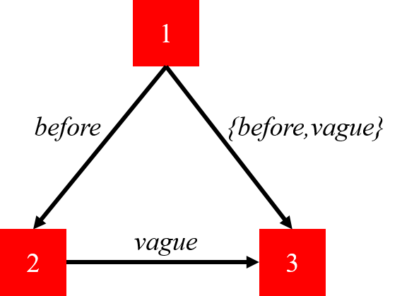
Figure 1: Nodes 1-3 are three time points and let $(i,j)$ be the edge from node $i$ to node $j$, where $(i,j)\in${before, after, equal, vague}. Assume the current annotation is $(1,2)=before$ and $(2,3)=vague$ and $(1,3)$ is missing. However, $(1,3)$ cannot be after because it leads to $(2,3)=after$, conflicting with their current annotation; similarly, $(1,3)$ cannot be equal, either.

A standard way to perform global inference is to formulate it as an Integer Linear Programming (ILP) problemRoth and Yih (2004) and enforce transitivity rules as constraints. Let $\mathcal{R}$ be the TempRel label set, $\mathcal{I}_{r}(ij)\in\{0,1\}$ be the indicator function of $(i,j)=r$, and $f_{r}(ij)\in[0,1]$ be the corresponding soft-max score obtained via $\mathcal{S}_{\mathcal{F+P}}$. Then the ILP objective is formulated as

$$\hat{\mathcal{I}}=\textrm{arg}\underset{\mathcal{I}}{\textrm{max}}\sum_{i<j}\sum_{r\in\mathcal{R}}f_{r}(ij)\mathcal{I}_{r}(ij)$$ (1)

$$\textrm{s.t.}\quad\underset{\textrm{(uniqueness)}}{\Sigma_{r}{\mathcal{I}_{r}(ij)}=1},$$

$$\underset{\textrm{(transitivity)}}{\mathcal{I}_{r_{1}}(ij)+\mathcal{I}_{r_{2}}(jk)-\Sigma_{m=1}^{N}\mathcal{I}_{r_{3}^{m}}(ik)\leq 1,}$$

where $\{r_{3}^{m}\}$ is selected based on the general transitivity proposed in Ning et al. (2017). With Eq. (1), different implementations of Line 1 in Algorithm 1 can be described concisely as follows: (i) Local inference is performed by ignoring “transitivity constraints”. (ii) Global inference can be performed by adding annotated edges in $\mathcal{P}$ as additional constraints. Note that Algorithm 1 is only for the learning step of TempRel extraction; as for the inference step of this task, we consistently adopt the standard method by solving Eq. (1), as was done by Bramsen et al. (2006); Chambers and Jurafsky (2008); Denis and Muller (2011); Do et al. (2012); Ning et al. (2017).

4 Experiments

In this work, we consistently used TB-Dense as the fully annotated dataset ($\mathcal{F}$) and TBAQ as the partially annotated dataset ($\mathcal{P}$). The corpus statistics of these two datasets are provided in Table 1. Note that TBAQ is the union of TimeBank and AQUAINT and it originally contained 256 documents, but 36 out of them completely overlapped with TB-Dense, so we have excluded these when constructing $\mathcal{P}$. In addition, the number of edges shown in Table 1 only counts the event-event relations (i.e., do not consider the event-time relations therein), which is the focus of this work.

Data	#Doc	#Edges	Ratio	Type
TB-Dense	36	6.5K	100%	$\mathcal{F}$
TBAQ	220	2.7K	12%	$\mathcal{P}$

Table 1: Corpus statistics of the fully and partially annotated dataset used in this work. TBAQ: The union of TimeBank and AQUAINT, which is the training set provided by the TempEval3 workshop. #Edges: The number of annotated edges. Ratio: The proportion of annotated edges.

We also adopted the original split of TB-Dense (22 documents for training, 5 documents for development, and 9 documents for test). Learning parameters were tuned to maximize their corresponding F-metric on the development set. Using the selected parameters, systems were retrained with development set incorporated and evaluated against the test split of TB-Dense (about 1.4K relations: 0.6K vague, 0.4K before, 0.3K after, and 0.1K for the rest). Results are shown in Table 2, where all systems were compared in terms of their performances on “same sentence” edges (both nodes are from the same sentence), “nearby sentence” edges, all edges, and the temporal awareness metric used by the TempEval3 workshop.

No.	Training		Same Sentence			Nearby Sentence			Overall			Awareness
	Data	Bootstrap	P	R	F	P	R	F	P	R	F	P	R	F
1	$\mathcal{F}$	-	47.1	49.7	48.4	40.2	37.9	39.0	42.1	41.0	41.5	40.0	40.7	40.3
2	$\mathcal{P}^{Full}$	-	37.0	33.1	35.0	34.4	19.6	24.9	37.7	23.6	29.0	36.9	24.0	29.1
3	$\mathcal{P}$	-	34.1	52.5	41.3	26.1	48.1	33.8	30.2	52.1	38.2	28.6	49.9	36.4
4	$\mathcal{F}$+$\mathcal{P}^{Full}$	-	38.5	32.2	35.1	40.1	38.1	39.1	40.8	35.3	37.8	37.1	36.2	36.6
5	$\mathcal{F}$+$\mathcal{P}$	-	43.7	43.9	43.8	39.1	38.3	38.7	41.8	40.7	41.2	38.6	41.4	40.0
6	$\mathcal{F}$+$\mathcal{P}^{Empty}$	Local	41.7	50.3	45.6	39.5	48.1	43.4	41.8	50.4	45.7	40.9	47.5	43.9
7	$\mathcal{F}$+$\mathcal{P}^{Empty}$	Global	44.7	55.5	49.5	40.1	48.7	44	42.0	51.4	46.2	41.1	48.3	44.4
8	$\mathcal{F}$+$\mathcal{P}$	Local	43.6	50	46.6	43	46.9	44.8	43.7	47.8	45.6	42	45.6	43.7
9	$\mathcal{F}$+$\mathcal{P}$	Global	44.9	56.1	49.9	43.4	52.3	47.5	44.7	54.1	49.0	44.1	50.8	47.2

Table 2: Performance of various usages of the partially annotated data in training. $\mathcal{F}$: Fully annotated data. $\mathcal{P}$: Partially annotated data. $\mathcal{P}^{Full}$: $\mathcal{P}$ with missing annotations filled by vague. $\mathcal{P}^{Empty}$: $\mathcal{P}$ with all annotations removed. Bootstrap: referring to specific implementations of Line 1 in Algorithm 1, i.e., local or global. Same/nearby sentence: edges whose nodes appear in the same/nearby sentences in text. Overall: all edges. Awareness: the temporal awareness metric used in the TempEval3 workshop, measuring how useful the predicted graphs are UzZaman et al. (2013). System 7 can also be considered as a reproduction of Ning et al. (2017) (see the discussion in Sec. 5 for details).

The first part of Table 2 (Systems 1-5) refers to the baseline method proposed at the beginning of Sec. 3, i.e., simply treating $\mathcal{P}$ as $\mathcal{F}$ and training on their union. $\mathcal{P}^{Full}$ is a variant of $\mathcal{P}$ by filling its missing edges by vague. Since it labels too many vague TempRels, System 2 suffered from a low recall. In contrast, $\mathcal{P}$ does not contain any vague training examples, so System 3 would only predict specific TempRels, leading to a low precision. Given the obvious difference in $\mathcal{F}$ and $\mathcal{P}^{Full}$, System 4 expectedly performed worse than System 1. However, when we see that System 5 was still worse than System 1, it is surprising because the annotated edges in $\mathcal{P}$ are correct and should have helped. This unexpected observation suggests that simply adding the annotated edges from $\mathcal{P}$ into $\mathcal{F}$ is not a proper approach to learn from both.

The second part (Systems 6-7) serves as an ablation study showing the effect of bootstrapping only. $\mathcal{P}^{Empty}$ is another variant of $\mathcal{P}$ we get by removing all the annotated edges (that is, only nodes are kept). Thus, they did not get any information from the annotated edges in $\mathcal{P}$ and any improvement came from bootstrapping alone. Specifically, System 6 is the standard bootstrapping and System 7 is the constrained bootstrapping.

Built on top of Systems 6-7, Systems 8-9 further took advantage of the annotations of $\mathcal{P}$, which resulted in additional improvements. Compared to System 1 (trained on $\mathcal{F}$ only) and System 5 (simply adding $\mathcal{P}$ into $\mathcal{F}$), the proposed System 9 achieved much better performance, which is also statistically significant with p$<$0.005 (McNemar’s test). While System 7 can be regarded as a reproduction of Ning et al. (2017), the original paper of Ning et al. (2017) achieved an overall score of P=43.0, R=46.4, F=44.7 and an awareness score of P=42.6, R=44.0, and F=43.3, and the proposed System 9 is also better than Ning et al. (2017) on all metrics.

5 Discussion

While incorporating transitivity constraints in inference is widely used, Ning et al. (2017) proposed to incorporate these constraints in the learning phase as well. One of the algorithms proposed in Ning et al. (2017) is based on Chang et al. (2012)’s constraint-driven learning (CoDL), which is the same as our intermediate System 7 in Table 2; the fact that System 7 is better than System 1 can thus be considered as a reproduction of Ning et al. (2017). Despite the technical similarity, this work is motivated differently and is set to achieve a different goal: Ning et al. (2017) tried to enforce the transitivity structure, while the current work attempts to use imperfect signals (e.g., partially annotated) taken from additional data, and learn in the incidental supervision framework.

The $\mathcal{P}$ used in this work is TBAQ, where only 12% of the edges are annotated. In practice, every annotation comes at a cost, either time or the expenses paid to annotators, and as more edges are annotated, the marginal “benefit” of one edge is going down (an extreme case is that an edge is of no value if it can be inferred from existing edges). Therefore, a more general question is to find out the optimal ratio of graph annotations.

Moreover, partial annotation is only one type of annotation imperfection. If the annotation is noisy, we can alter the hard constraints derived from $\mathcal{P}$ and use soft regularization terms; if the annotation is for a different but relevant task, we can formulate corresponding constraints to connect that different task to the task at hand. Being able to learn from these “indirect” signals is appealing because indirect signals are usually order of magnitudes larger than datasets dedicated to a single task.

6 Conclusion

Temporal relation (TempRel) extraction is important but TempRel annotation is labor intensive. While fully annotated datasets ($\mathcal{F}$) are relatively small, there exist more datasets with partial annotations ($\mathcal{P}$). This work provides the first investigation of learning from both types of datasets, and this preliminary study already shows promise. Two bootstrapping algorithms (standard and constrained) are analyzed and the benefit of $\mathcal{P}$, although with missing annotations, is shown on a benchmark dataset. This work may be a good starting point for further investigations of incidental supervision and data collection schemes of the TempRel extraction task.

References

- Bethard (2013) Steven Bethard. 2013. ClearTK-TimeML: A minimalist approach to TempEval 2013. In Second Joint Conference on Lexical and Computational Semantics (* SEM). volume 2, pages 10–14.
- Bethard et al. (2007) Steven Bethard, James H Martin, and Sara Klingenstein. 2007. Timelines from text: Identification of syntactic temporal relations. In IEEE International Conference on Semantic Computing (ICSC). pages 11–18.
- Bethard et al. (2016) Steven Bethard, Guergana Savova, Wei-Te Chen, Leon Derczynski, James Pustejovsky, and Marc Verhagen. 2016. SemEval-2016 Task 12: Clinical TempEval. In Proceedings of the 10th International Workshop on Semantic Evaluation (SemEval-2016). Association for Computational Linguistics, San Diego, California, pages 1052–1062.
- Bethard et al. (2017) Steven Bethard, Guergana Savova, Martha Palmer, and James Pustejovsky. 2017. SemEval-2017 Task 12: Clinical TempEval. In Proceedings of the 11th International Workshop on Semantic Evaluation (SemEval-2017). Association for Computational Linguistics, pages 565–572.
- Bramsen et al. (2006) P. Bramsen, P. Deshpande, Y. K. Lee, and R. Barzilay. 2006. Inducing temporal graphs. In Proceedings of the Conference on Empirical Methods for Natural Language Processing (EMNLP). pages 189–198.
- Cassidy et al. (2014) Taylor Cassidy, Bill McDowell, Nathanel Chambers, and Steven Bethard. 2014. An annotation framework for dense event ordering. In Proceedings of the Annual Meeting of the Association for Computational Linguistics (ACL). pages 501–506.
- Chambers and Jurafsky (2008) N. Chambers and D. Jurafsky. 2008. Jointly combining implicit constraints improves temporal ordering. In Proceedings of the Conference on Empirical Methods for Natural Language Processing (EMNLP).
- Chambers (2013) Nate Chambers. 2013. NavyTime: Event and time ordering from raw text. In Second Joint Conference on Lexical and Computational Semantics (*SEM), Volume 2: Proceedings of the Seventh International Workshop on Semantic Evaluation (SemEval 2013). Association for Computational Linguistics, Atlanta, Georgia, USA, pages 73–77.
- Chambers et al. (2014) Nathanael Chambers, Taylor Cassidy, Bill McDowell, and Steven Bethard. 2014. Dense event ordering with a multi-pass architecture. Transactions of the Association for Computational Linguistics 2:273–284.
- Chambers et al. (2007) Nathanael Chambers, Shan Wang, and Dan Jurafsky. 2007. Classifying temporal relations between events. In Proceedings of the 45th Annual Meeting of the ACL on Interactive Poster and Demonstration Sessions. pages 173–176.
- Chang et al. (2012) M. Chang, L. Ratinov, and D. Roth. 2012. Structured learning with constrained conditional models. Machine Learning 88(3):399–431.
- Denis and Muller (2011) Pascal Denis and Philippe Muller. 2011. Predicting globally-coherent temporal structures from texts via endpoint inference and graph decomposition. In Proceedings of the International Joint Conference on Artificial Intelligence (IJCAI). volume 22, page 1788.
- Do et al. (2012) Q. Do, W. Lu, and D. Roth. 2012. Joint inference for event timeline construction. In Proc. of the Conference on Empirical Methods in Natural Language Processing (EMNLP).
- Graff (2002) David Graff. 2002. The AQUAINT corpus of english news text. Linguistic Data Consortium, Philadelphia .
- Laokulrat et al. (2013) Natsuda Laokulrat, Makoto Miwa, Yoshimasa Tsuruoka, and Takashi Chikayama. 2013. UTTime: Temporal relation classification using deep syntactic features. In Second Joint Conference on Lexical and Computational Semantics (* SEM). volume 2, pages 88–92.
- Mani et al. (2006) Inderjeet Mani, Marc Verhagen, Ben Wellner, Chong Min Lee, and James Pustejovsky. 2006. Machine learning of temporal relations. In Proceedings of the Annual Meeting of the Association for Computational Linguistics (ACL). pages 753–760.
- Minard et al. (2015) Anne-Lyse Minard, Manuela Speranza, Eneko Agirre, Itziar Aldabe, Marieke van Erp, Bernardo Magnini, German Rigau, Ruben Urizar, and Fondazione Bruno Kessler. 2015. SemEval-2015 Task 4: TimeLine: Cross-document event ordering. In Proceedings of the 9th International Workshop on Semantic Evaluation (SemEval 2015). pages 778–786.
- Mirza and Tonelli (2016) Paramita Mirza and Sara Tonelli. 2016. CATENA: CAusal and TEmporal relation extraction from NAtural language texts. In The 26th International Conference on Computational Linguistics. pages 64–75.
- Mostafazadeh et al. (2016) Nasrin Mostafazadeh, Alyson Grealish, Nathanael Chambers, James Allen, and Lucy Vanderwende. 2016. CaTeRS: Causal and temporal relation scheme for semantic annotation of event structures. In Proceedings of the 4th Workshop on Events: Definition, Detection, Coreference, and Representation. pages 51–61.
- Ning et al. (2017) Qiang Ning, Zhili Feng, and Dan Roth. 2017. A structured learning approach to temporal relation extraction. In Proceedings of the Conference on Empirical Methods for Natural Language Processing (EMNLP). Copenhagen, Denmark.
- Ning et al. (2018a) Qiang Ning, Zhili Feng, Hao Wu, and Dan Roth. 2018a. Joint reasoning for temporal and causal relations. In Proceedings of the Annual Meeting of the Association for Computational Linguistics (ACL).
- Ning et al. (2018b) Qiang Ning, Hao Wu, Haoruo Peng, and Dan Roth. 2018b. Improving temporal relation extraction with a globally acquired statistical resource. In Proceedings of the Annual Meeting of the North American Association of Computational Linguistics (NAACL). Association for Computational Linguistics.
- Ning et al. (2018c) Qiang Ning, Hao Wu, and Dan Roth. 2018c. A multi-axis annotation scheme for event temporal relations. In Proceedings of the Annual Meeting of the Association for Computational Linguistics (ACL).
- O’Gorman et al. (2016) Tim O’Gorman, Kristin Wright-Bettner, and Martha Palmer. 2016. Richer event description: Integrating event coreference with temporal, causal and bridging annotation. In Proceedings of the 2nd Workshop on Computing News Storylines (CNS 2016). Association for Computational Linguistics, Austin, Texas, pages 47–56.
- Pustejovsky et al. (2003) James Pustejovsky, Patrick Hanks, Roser Sauri, Andrew See, Robert Gaizauskas, Andrea Setzer, Dragomir Radev, Beth Sundheim, David Day, Lisa Ferro, et al. 2003. The TIMEBANK corpus. In Corpus linguistics. volume 2003, page 40.
- Roth and Yih (2004) D. Roth and W. Yih. 2004. A linear programming formulation for global inference in natural language tasks. In Hwee Tou Ng and Ellen Riloff, editors, Proc. of the Conference on Computational Natural Language Learning (CoNLL). pages 1–8.
- Roth (2017) Dan Roth. 2017. Incidental supervision: Moving beyond supervised learning. In AAAI.
- UzZaman et al. (2013) Naushad UzZaman, Hector Llorens, James Allen, Leon Derczynski, Marc Verhagen, and James Pustejovsky. 2013. SemEval-2013 Task 1: TempEval-3: Evaluating time expressions, events, and temporal relations. In Second Joint Conference on Lexical and Computational Semantics. volume 2, pages 1–9.
- Verhagen et al. (2007) Marc Verhagen, Robert Gaizauskas, Frank Schilder, Mark Hepple, Graham Katz, and James Pustejovsky. 2007. SemEval-2007 Task 15: TempEval temporal relation identification. In SemEval. pages 75–80.
- Verhagen and Pustejovsky (2008) Marc Verhagen and James Pustejovsky. 2008. Temporal processing with the TARSQI toolkit. In 22nd International Conference on on Computational Linguistics: Demonstration Papers. pages 189–192.
- Verhagen et al. (2010) Marc Verhagen, Roser Sauri, Tommaso Caselli, and James Pustejovsky. 2010. SemEval-2010 Task 13: TempEval-2. In SemEval. pages 57–62.