PyMieDAP : a Python–Fortran tool to compute fluxes and polarization signals of (exo)planets

PyMieDAP (the Python Mie Doubling-Adding Programme) is a Python–based tool for computing the total, linearly, and circularly polarized fluxes of incident unpolarized sun- or starlight that is reflected by, respectively, Solar System planets or moons, or exoplanets at a range of wavelengths. The radiative transfer computations are based on an adding–doubling Fortran algorithm and fully include polarization for all orders of scattering. The model (exo)planets are described by a model atmosphere composed of a stack of homogeneous layers containing gas and/or aerosol and/or cloud particles bounded below by an isotropically, depolarizing surface (that is optionally black). The reflected light can be computed spatially–resolved and/or disk–integrated. Spatially–resolved signals are mostly representative for observations of Solar System planets (or moons), while disk–integrated signals are mostly representative for exoplanet observations. PyMieDAP is modular and flexible, and allows users to adapt and optimize the code according to their needs. PyMieDAP keeps options open for connections with external programs and for future additions and extensions. In this paper, we describe the radiative transfer algorithm that PyMieDAP is based on and the code’s principal functionalities. And we provide benchmark results of PyMieDAP that can be used for testing its installation and for comparison with other codes. PyMieDAP is available online under the GNU GPL license at http://gitlab.com/loic.cg.rossi/pymiedap

1 Introduction

Light is usually described only by its total flux, and usually, the total flux is the only parameter that is measured when observing sunlight that is reflected by the Earth or other planets in the Solar System. A full description of light, however, requires its state of polarization. The state of polarization includes the degree of polarization, $P$, i.e. the ratio of the polarized flux to the total –polarized plus unpolarized– flux, and the direction of polarization, $\chi$. The polarized flux can be subdivided into the linearly polarized flux and the circularly polarized flux. Similarly, the degree of polarization $P$ can be subdivided into the degree of linear polarization $P_{\rm l}$ and the degree of circular polarization $P_{\rm c}$. An excellent description of the polarization of light that is reflected by planetary atmospheres and surfaces can be found in Hansen & Travis (1974). That paper also includes various methods to compute the state of polarization of light that is reflected by a planet, amongst others the so–called adding–doubling method, that is employed by PyMieDAP, the code that is the topic of this paper.

There are several reasons for measuring the state of polarization of sunlight that is reflected by a planet, or starlight that is reflected by an exoplanet. A first advantage of polarimetry comes from the fact that the light of a solar type star can be considered to be unpolarized when integrated across the stellar disk. This is known to be true for our Sun (Kemp et al., 1987), and is also supported by other studies of nearby FGK stars: for example, Cotton et al. (2017) show that while active stars can present polarizations up to 45 ppm, non-active stars have very limited and practically negligeable intrinsic polarisation.

Meanwhile, light that is scattered within a planetary atmosphere and/or that is reflected by the planetary surface will usually be (linearly) polarized. For exoplanets, polarimetry could thus allow distinguishing the very faint planetary signal from the much brighter stellar light. In addition, the measurement of a polarized signal would immediately confirm the nature of the object. Seager et al. (2000) present numerically simulated degrees of (linear) polarization of the combined light of a star and various types of orbiting gaseous planets. When planets are spatially unresolved from their star, the degree of polarization of the system as a whole is the ratio of the polarized planetary flux to the sum of the total planetary flux and the stellar flux. This degree of polarization is obviously very small, i.e. on the order of $10^{-6}$ (Seager et al., 2000). Stam et al. (2004) present numerically simulated degrees of (linear) polarization of spatially resolved gaseous planets. For these planets, the degree of polarization can reach several tens of percent, depending on the physical properties of the planet and the planetary phase angle, because they do not include the huge, unpolarized stellar signal. Clearly, the degree of polarization that can be observed for a given exoplanet will depend not only on the intrinsic degree of polarization of the planet, but also on the stellar flux in the background of the planetary signal.

Another interesting use of polarimetry is the characterization of the planetary object. The degree and direction of polarization of light that has been scattered by a planet (locally or disk–integrated) is very sensitive to the properties of the atmospheric scatterers (size, shape, composition), their spatial distribution, and/or to the reflection properties of the planetary surface (bidirectional reflection, albedo) (see e.g. Hansen & Travis, 1974; Mishchenko et al., 2002, and references therein), if present. In particular, multiple scattering of light randomizes and hence depolarizes the light, and adds mainly unpolarized light to the reflected signal. The angular dependence of the degree and direction of polarization of the reflected signal thus preserves the angular patterns of the light that is singly scattered by the atmospheric particles or the surface, and that is characteristic for the microphysical properties of the scatterers. A famous application of the use of polarimetry for the characterization of a planetary atmosphere is the retrieval of the composition and size of the cloud particles in Venus’ upper clouds using disk–integrated polarimetry (with Earth–based telescopes) at a range of phase angles and several wavelengths (Hansen & Hovenier, 1974). This information could not be derived from total flux measurements, because the total flux is less sensitive to the composition and size of the scattering particles. Indeed, various types of cloud particles would provide a fit to the total flux measurements.

Even if one were not interested in measurements of polarization and the analysis of polarization data, there are compelling reasons to include polarization in the computation of total fluxes.

Firstly, because light is fully described by a vector and scattering processes by matrices, ignoring polarization can induce errors up to several percent in computed total fluxes both locally and disk–integrated (Mishchenko et al., 1994; Stam & Hovenier, 2005). In particular, in gaseous absorption bands, where the linear polarization usually differs from the polarization in the continuum (Fauchez et al., 2017; Boesche et al., 2009; Stammes et al., 1994; Aben et al., 1997), such errors will lead to errors in derived gas mixing ratios and e.g. cloud top altitudes (Stam & Hovenier, 2005).

Secondly, many spectrometers are sensitive to the state of polarization of the incoming light because of the optical properties of mirrors and e.g. gratings. Knowing the polarization sensitivity of your instrument, for example, through calibration in an optical laboratory, is not sufficient to correct total flux measurements for the state of polarization of the incoming light if the polarization of the light is not known (Stam et al., 2000). However, one could include the computed state of polarization of the observed light, combined with the instrument’s polarization sensitivity in the retrieval of the total fluxes.

A reason why polarization is usually ignored in radiative transfer computations is probably that codes that fully include polarization for all orders of scattering are more complex than codes that ignore polarization, because the latter treat light as a scalar and scattering processes as described by scalars, while the former have to use vectors and matrices. Polarized radiative transfer codes therefore usually also require more computation time than scalar codes.

In this paper, we present PyMieDAP, a user–friendly, modular, Python–based tool for computing the total and polarized fluxes of light that is reflected by (exo)planets. The radiative transfer computations in PyMieDAP are performed with an adding–doubling algorithm written in Fortran, as described by (de Haan et al., 1987), while input and output are handled with Python code. Figure 1 provides a view of the modules composing PyMieDAP. The blue boxes represent codes written in Fortran, and the red boxes Python code. Arrows indicate interfaces using f2py (Peterson, 2009). Each PyMieDAP module will be described in more detail in this paper.

Figure 1: The modules comprising PyMieDAP. The blue boxes represent Fortran codes, the red boxes Python codes.

The structure of this paper is as follows. Section 2 provides the definitions of the vector elements that describe the state of polarization of light as used in PyMieDAP. Section 3 contains the formulae required to calculate the Stokes vectors of sun- or starlight that is locally reflected by a region on a planet for a range of illumination and viewing geometries. The components of the Fourier–series decomposition of these vectors are stored in files in a database that is accessed to compute reflected light vectors for specific geometries. Section 4 describes the computation of the single scattering properties of atmospheric gases and aerosols, and the reflection by the surface. Section 5 describes the adding–doubling radiative transfer algorithm used in PyMieDAP . Section 6 presents the method used to compute the geometries for locally reflected light, and describes how previously stored database files are used to compute the locally reflected light vector as well as how to integrate these locally reflected light vectors across the illuminated and visible part of a planetary disk, in order to obtain the disk–integrated Stokes vector. In Sect. 7, we compare reflected Stokes vectors obtained with PyMieDAP against previously published results obtained using a similar adding–doubling radiative transfer algorithm without the intermediate step of using pre–calculated database files, and without the Python shell. Section 8 summarizes the paper and discusses future work. Appendix A provides a detailed description of the format of the database files that is used in the codes. Appendix B provides equations for the computation of some angles used in the code.

2 Defining the flux and polarization of light

The radiance (’intensity’) and state of polarization of a quasi–monochromatic beam of light can be described by a Stokes vector ${\bf I}$ as follows (see, e.g. Hansen & Travis, 1974; Hovenier et al., 2004)

$${\bf I}=\left[\begin{array}[]{c}I\\ Q\\ U\\ V\end{array}\right].$$ (1)

Here, Stokes parameter $I$ is the total radiance, $Q$ and $U$ describe the linearly polarized radiances, and $V$ the circularly polarized radiance. All four parameters have the dimension W m^-2 sr^-1 (or W m^-3 sr^-1 if taken as functions of the wavelength $\lambda$). We will also use the irradiance or flux vector $\pi{\bf F}=\pi[F,Q,U,V]$, of which all parameters have the dimension W m^-2 (or W m^-3 if taken as functions of $\lambda$). Unless specified otherwise, the equations in this paper also hold for flux vector $\pi{\bf F}$.

Parameters $Q$ and $U$ are defined with respect to a reference plane. We use two types of reference planes:

1. The local meridian plane, which contains the local zenith direction and the direction of propagation of the light. The local meridian plane is used in the computation of $Q$ and $U$ of locally reflected light.

2. The planetary scattering plane, which contains the centre of the planet, and the directions to the centre of the star and to the observer. This plane is mainly used to define $Q$ and $U$ of light that has been reflected by the planet as a whole, e.g. for simulating signals of (spatially unresolved) exoplanets.

Parameters $Q$ and $U$ can be transformed from one reference plane to another using a so–called rotation matrix ${\bf L}$ (see Hovenier & van der Mee, 1983)

$${\bf L}(\beta)=\left[\begin{array}[]{cccc}1&0&0&0\\ 0&\cos 2\beta&\sin 2\beta&0\\ 0&-\sin 2\beta&\cos 2\beta&0\\ 0&0&0&1\\ \end{array}\right],$$ (2)

with $\beta$ the angle between the two reference planes, measured rotating in the anti–clockwise direction from the old to the new reference plane when looking towards the observer ($\beta\geq 0^{\circ}$).

In PyMieDAP, the default reference plane for local reflections and disk–integrated reflected light, is the planetary scattering plane. For locally reflected light, the vector that is computed with respect to the local meridian plane is rotated to be defined with respect to the planetary scattering plane before being provided as output. As a planet orbits its star, the planetary scattering plane will usually rotate on the sky as seen from the observer, except if the orientation of the orbit is edge–on with respect to the observer (see Fig. 2). By applying additional rotations, Stokes vectors defined with respect to the planetary scattering plane can straightforwardly be redefined to e.g. the optical plane of an instrument or the detector (for a detailed description of these rotations, see Rossi & Stam, 2017).

Figure 2: Illustration of the rotation of the planetary scattering plane for an orbit with a random orientation (left) and with edge-on configuration (right). The first case would require further rotations to express the Stokes elements in the reference plane of the observer.

The degree of polarization of the beam of light described by vector ${\bf I}$ (Eq. 1) is defined as

$$P=\frac{\sqrt{Q^{2}+U^{2}+V^{2}}}{I}.$$ (3)

The degree of linear polarization is defined as

$$P_{\rm l}=\frac{\sqrt{Q^{2}+U^{2}}}{I},$$ (4)

and the degree of circular polarization as

$$P_{\rm c}=\frac{V}{I}.$$ (5)

While the degree of linear polarization is independent of the choice of reference plane for Stokes parameters $Q$ and $U$, the direction or angle of linear polarization, $\chi$, is not independent of the choice of reference plane. Angle $\chi$ can be derived from

$$\tan 2\chi=U/Q.$$ (6)

The value of $\chi$ is chosen in the interval $[0^{\circ},180^{\circ}\rangle$, and such that $\cos 2\chi$ has the same sign as $Q$ (see Hansen & Travis, 1974).

If $U=0$, the direction of polarization of the light is either perpendicular ($Q<0$, $\chi=90^{\circ}$) or parallel ($Q>0$, $\chi=0^{\circ}$) to the reference plane. In that case, we can use an alternative definition of the degree of linear polarization that captures the information about the direction of polarization, namely

$$P_{\rm ls}=-\frac{Q}{I},$$ (7)

where $P_{\rm ls}>0$ ($P_{\rm ls}<0$) corresponds with light that is polarized perpendicularly (parallel) to the reference plane.

Regarding the circular polarization (Eq. 5), our convention for the sign is as follows: $V$ and thus $P_{\rm c}$ is positive when the observer ’sees’ the electric vector of the light rotating in the anti–clockwise direction, and $V$ and thus $P_{\rm c}$ is negative, when the observer ’sees’ the vector rotating in the clockwise direction.

3 Calculating reflected light

With PyMieDAP, one can calculate the Stokes vector ${\bf I}$ (cf. Eq. 1) of light that is locally reflected by a planet. Here, we refer to locally reflected light if a single combination of illumination and viewing geometries involved in the reflection process applies. With PyMieDAP, one can also integrate Stokes vectors of locally reflected light across the planet, taking into account variations of the atmospheric properties and/or surface albedo, as well as the variations of the illumination and viewing geometries.

Below, we explain the calculation of the locally reflected light (Sect. 3.1) and the integration of locally reflected light across the illuminated and visible part of a planetary disk (Sect. 3.2). The integration over a smaller part of a planet could straightforwardly be derived from the latter explanation.

3.1 Calculating locally reflected light

We calculate a locally reflected vector ${\bf I}$ (see Eq. 1) according to (see Hansen & Travis, 1974)

$${\bf I}(\mu,\mu_{0},\phi-\phi_{0},\lambda)=\mu_{0}\hskip 2.84544pt{\bf R}(\mu,\mu_{0},\phi-\phi_{0},\lambda)\hskip 2.84544pt{\bf F}_{0}(\lambda),$$ (8)

with ${\bf F}_{0}$ the vector describing the incident light and ${\bf R}$ the $4\times 4$ local planetary reflection matrix. The reference plane for ${\bf I}$ is the local meridian plane, the plane containing the local zenith direction and the propagation direction of the reflected light (see Sect. 2).

Furthermore in Eq. 8, $\mu=\cos\theta$, with $\theta$ the angle between the direction of propagation of the reflected light and the upward vertical ($0^{\circ}\leq\theta<90^{\circ}$), and $\mu_{0}=\cos\theta_{0}$, with $\theta_{0}$ the angle between the upward vertical and the direction to the sun or star ($0^{\circ}\leq\theta_{0}<90^{\circ}$). The azimuthal difference angle $\phi-\phi_{0}$ is measured between the two vertical planes containing the directions of propagation of the reflected and the incident light, respectively ($0^{\circ}\leq\phi-\phi_{0}\leq 180^{\circ}$). To get our definition for $\phi-\phi_{0}$ clear, consider light that is reflected in the vertical plane that contains the local zenith direction, and the direction towards the sun or star. If the reflected light propagates in the half of the vertical plane that contains the sun or star, $\phi-\phi_{0}=180^{\circ}$. If the reflected light propagates in the other half of the plane, $\phi-\phi_{0}=0^{\circ}$.

In PyMieDAP, it is assumed that the incident sun or starlight is unpolarized (Kemp et al., 1987), although this assumption is not inherent to the radiative transfer algorithm (de Haan et al., 1987), and PyMieDAP could easily be adapted for polarized incident light. Vector ${\bf F}_{0}$ of the light that is incident on a model planet thus equals the column vector $[F_{0},0,0,0]$ or $F_{0}[1,0,0,0]$, where $F_{0}$ equals the total incident solar/stellar flux measured perpendicular to the direction of incidence divided by $\pi$ (see Hansen & Travis, 1974). For example, if the total incident flux measured perpendicular to the direction of incidence equals $S_{0}$ W m^-2, $F_{0}=S_{0}/\pi$ W m^-2.

With the assumption of unpolarized incident sun or starlight, only the elements of ${\bf R}_{1}$, the first column of the $4\times 4$ local planetary reflection matrix ${\bf R}$ are relevant for the calculation of the locally reflected vector ${\bf I}$, since Eq. 8 then transforms into

$${\bf I}(\mu,\mu_{0},\phi-\phi_{0},\lambda)=\mu_{0}\hskip 2.84544pt{\bf R}_{1}(\mu,\mu_{0},\phi-\phi_{0},\lambda)\hskip 2.84544ptF_{0}(\lambda).$$ (9)

The local reflection vector ${\bf R}_{1}$ depends on the illumination and viewing geometries and the properties of the local planetary atmosphere and surface. The user can provide PyMieDAP with a list of illumination and viewing geometries, e.g. geometries that pertain to observations from a satellite that orbits a planet. Given the properties of the local atmosphere and surface, the calculation of ${\bf R}_{1}$ and subsequently ${\bf I}$ is performed by PyMieDAP as described in Sect. 5. Note that locally reflected light vector ${\bf I}$ as described by Eq. 9 is defined with respect to the local meridian plane. PyMieDAP will redefine it with respect to the planetary scattering plane by calculating the local angle $\beta$ and applying the rotation matrix ${\bf L}$ as defined in Eq. 2.

In case circular polarization is ignored, vector ${\bf R}_{1}$ and reflected light vector ${\bf I}$ each comprise only 3 elements. In case circular and linear polarization are both ignored, ${\bf R}_{1}$ and ${\bf I}$ are scalars, and Eq. 9 could be written as

$$I(\mu,\mu_{0},\phi-\phi_{0},\lambda)=\mu_{0}\hskip 2.84544ptR_{1}(\mu,\mu_{0},\phi-\phi_{0},\lambda)\hskip 2.84544ptF_{0}(\lambda).$$ (10)

Contrary to ignoring linear polarization, ignoring circular polarization usually only leads to very small errors in the computed total and linearly polarized fluxes (Hovenier & Stam, 2005).

In the following, we will assume polarization (both linear and circular) is taken into account and use vectors and matrices instead of scalars.

3.2 Calculating disk–integrated reflected light

To calculate signals of spatially unresolved planets, such as exoplanets, we integrate the locally reflected starlight as given by Eqs. 9 and 10, over the illuminated and visible part of the planetary disk, according to (see Stam et al., 2006, Eq. 16)

$$\pi{\bf F}(\alpha,\lambda) = \frac{1}{d^{2}}\int_{\rightmoon}\mu{\bf L}(\beta){\bf I}(\mu,\mu_{0},\phi-\phi_{0},\lambda)dO$$ (11)

$$= \frac{1}{d^{2}}\int_{\rightmoon}\mu\mu_{0}{\bf L}(\beta){\bf R}_{1}(\mu,\mu_{0},\phi-\phi_{0},\lambda)F_{0}(\lambda)dO.$$ (12)

Here, $\pi{\bf F}$ is the flux vector of the reflected starlight as it arrives at the observer located at a distance $d$ from the planet, with $\pi F$ the flux measured perpendicularly to the direction of propagation of the light. Furthermore, $\mu\hskip 2.84544ptdO/d^{2}$ is the solid angle under which surface area $dO$ on the planet is seen by the observer ($\mu=\cos\theta$). The planet’s radius $r$ is incorporated in the surface integral (the planet is thus not assumed to be a unit sphere). Reflected light vector $\pi{\bf F}$ depends on the planetary phase angle $\alpha$, i.e. the angle between the star and the observer as measured from the centre of the planet ($0^{\circ}\leq\alpha\leq 180^{\circ}$). The range of observable phase angles for an exoplanet will depend on the orbital inclination and/or on the inner working angle of the instrument.

Furthermore in Eq. 12, each locally reflected vector ${\bf I}$, and hence each local reflection matrix ${\bf R}_{1}$ is rotated such that the reference plane is no longer the local meridian plane, but the planetary scattering plane. The local rotation angle $\beta$ depends on the local viewing angle $\theta$ and the location of surface area $dO$ on the planet.

The geometric albedo $A_{\rm G}$ of the planet with radius $r$ at distance $d$ is given by

$$A_{\rm G}(\lambda)=\frac{\pi F(0^{\circ},\lambda)}{\pi F_{0}}(\lambda)\frac{d^{2}}{r^{2}},$$ (13)

where $\pi F_{0}(0^{\circ},\lambda)$ is the reflected total flux at wavelength $\lambda$ and phase angle $\alpha$ equal to $0^{\circ}$.

In PyMieDAP, the integration in Eq. 12 is replaced by a summation over locally reflected Stokes vectors. In order to do so, we divide the planetary disk on the sky in pixels, and compute the locally reflected Stokes vector at the centre of each pixel. A pixel contributes to the disk–signal when its center is within the disk–radius. The integration is then given by:

$$\pi{\bf F}(\alpha,\lambda)=\frac{F_{0}(\lambda)}{d^{2}}\sum_{n=1}^{N}\mu_{n}\hskip 2.84544pt\mu_{0n}\hskip 2.84544pt{\bf L}(\beta_{n})\hskip 2.84544pt{\bf R}_{1}(\mu_{n},\mu_{0n},\phi_{n}-\phi_{0n},\lambda)\hskip 2.84544ptdO_{n},$$ (14)

with $N$ the number of illuminated and visible pixels on the planetary disk, and with subscript $n$ indicating that $\mu$, $\mu_{0}$, $\phi-\phi_{0}$, and $\beta$ depend on the location of the pixel on the planet. In addition, $\mu_{0}$, $\phi-\phi_{0}$, and $\beta$ at a given location of the pixel on the planet depend on the planet’s phase angle $\alpha$ (Appendix B provides relations that can be used to derive these angles). In the summation, $dO_{n}$ refers to the area of the pixel as measured on the surface of the planet.

Although not explicitly indicated in Eqs. 14 and 12, ${\bf R}_{1}$ will usually also depend on the location (of a pixel) on the planet. Typical horizontally inhomogeneities would be: the surface coverage and altitude, and the atmospheric composition and structure. The obvious horizontal variations on Earth are of course the oceans and the continents, and in the atmosphere, the clouds. Horizontal inhomogeneities can be taken into account by using different local reflection vectors ${\bf R}_{1}$ across the planet (in that case, ${\bf R}_{1}$ in Eq. 14 would include a subscript $n$).

Given a model planet and a planetary phase angle $\alpha$, the steps to evaluate Eq. 14, are the following:

1. Divide the planet in pixels small enough to be able to assume that the planet properties across each pixel are horizontally homogeneous, and to be able to follow the limb and the terminator of the planet.

2. Calculate for (the centre of) each pixel the angles $\mu$ (i.e. $\cos\theta$), $\phi$, and the rotational angle $\beta$. These angles are independent of the location of the sun or star with respect to the planet.

3. Calculate for the given phase angle $\alpha$, and for (the centre of) each pixel, $\mu_{0}$ (i.e. $\cos\theta_{0}$) and $\phi_{0}$. These angles depend on the location of the sun or star with respect to the planet.

4. Calculate for (the centre of) each pixel, the column vector ${\bf R}_{1}$ of the locally reflected light using the appropriate database file (see Sect. 5).

5. Perform the summation described by Eq. 14.

The pixels can be defined on the planet, for example by using a latitude and longitude grid, in which case $\mu\hskip 2.84544ptdO$, the projected area of the pixel (see Eq. 12), i.e. the pixel area as ’seen’ by the observer (see Fig. 3) will depend on the location of the pixel on the planet. PyMieDAP uses a grid of equally sized square pixels, similar to detector pixels, and uses the projections of those pixels onto the planet to divide the planet into separate regions. In this case, $\mu\hskip 2.84544ptdO$ is simply the surface area of the square pixel, and there is no need to calculate $dO$, the surface of the projected pixel on the planet (which can have a complicated shape). The result of the integration will depend on the pixel size, and thus on the number of pixels across the planetary disk, in particular at large phase angles, where the pixels should be sufficiently small resolve the crescent shape of the illuminated part of the planetary disk.

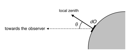
Figure 3: Sketch of a surface area $dO$ on the planet (side view) and its projection towards the observer. The observer ’sees’ a pixel area equal to $\mu\hskip 2.84544ptdO=\cos\theta\hskip 2.84544ptdO$, with $\theta$ the local viewing zenith angle.

The computation time increases linearly with $N$, the number of pixels on the illuminated and visible part of the planetary disk. In order to keep computing times low, it is thus important to find a balance between the number of pixels and the accuracy. The relative error in the total flux of a Lambertian reflecting planet due to the pixel size is shown in Fig. 4. The errors decrease with increasing value of $N$ at any given phase angle $\alpha$. For a given value of $N$, the relative error increases with increasing phase angle $\alpha$, thus with decreasing width of the planetary crescent, but the total disk–integrated flux also decreases with increasing $\alpha$, with $\pi F(180^{\circ})=0.0$. Thus while the relative errors at large phase angles can be very large, the absolute errors remain small. For computations across a range of phase angles, PyMieDAP can automatically increase the number of pixels across the equator $N_{\rm eq}$ (and therefore $N$) with increasing $\alpha$ in order to keep the errors small. The results of this automatic increase of $N$ are also shown in Fig. 4. This ’adaptive pixels scheme’ can be useful as a trade-off between computational efficiency and the need to resolve the planet at large phase angles, as using a smaller number of pixels for a full planet is usually acceptable, while it might be detrimental to the computed output for thin crescents.

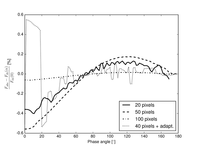
Figure 4: The difference between the disk–integrated flux $F$ computed using Eq. 14 and computed using the analytical expression for a sphere with a Lambertian reflecting surface and a geometric albedo $A_{\rm G}$ of 1.0 (see Stam et al., 2006, and Eq. 39), as a function of the planet’s phase angle $\alpha$ for various values of $N_{\rm eq}$, the number of pixels along the planet’s equator. The difference has been normalized to $A_{\rm G}$. The dotted line: $N_{\rm eq}$ increases with $\alpha$ according to $N_{\rm eq}(\alpha)=N_{\rm eq}(0^{\circ})[1+\sin^{2}(\alpha/2)]$, with $N_{\rm eq}(0^{\circ})=40$.

Note that for horizontally homogeneous planets, the Stokes vector of the hemisphere above the planetary scattering plane equals that of the southern hemisphere, except for the sign of Stokes parameters $U$ and $V$.

For horizontally homogeneous planets, Stam et al. (2006) describe an efficient algorithm that does not require dividing the planet into pixels, and that evaluates the disk–integrated Stokes vector $\pi{\bf F}$ at arbitrary phase angles $\alpha$. With this algorithm (that has not been implemented in PyMieDAP), vectors of horizontally inhomogeneous planets can be approximated using a weighted sum of vectors of horizontally homogeneous planets (see Stam, 2008), with the weights depending on the fractions the various inhomogeneities cover on the illuminated and visible part of the planetary disk. With such a weighted sum approximation, one can estimate the range of signals to be expected from an exoplanet. However, because a weighted sum does not account for the actual spatial distribution of the inhomogeneities, and e.g. the change therein when a planet rotates about its axis, it cannot be used for interpreting signals of planets that are known to exhibit significant horizontal inhomogeneities. For such applications, PyMieDAP’s pixel approach should be used.

4 Describing the model atmosphere and surface

PyMieDAP ’s adding–doubling radiative transfer algorithm assumes a flat model atmosphere that is horizontally homogeneous, but that can be vertically inhomogeneous because different horizontally homogeneous atmospheric layers can be stacked. A model atmosphere is bounded below by a flat, horizontally homogeneous surface. Below we describe how the scattering by the gaseous molecules, the aerosol particles and the reflection by the surface is implemented in PyMieDAP.

4.1 The model atmosphere

A model atmosphere consists of a stack of horizontally homogeneous layers. Each atmospheric layer can contain gaseous molecules and/or aerosol particles (including cloud particles). For every layer, the algorithm requires the total optical thickness $b$, the single scattering matrix ${\bf F}$ of the gas and/or aerosol particles in the layer, and their single scattering albedo $a$.

The single scattering of incident light by gas molecules is described by anisotropic Rayleigh scattering (Hansen & Travis, 1974), which includes both the inelastic Cabannes scattering and the elastic Raman scattering processes (Young, 1981). Although overall energy is thus conserved, narrow spectral features that are due to Raman scattering, such as the filling–in of absorption lines in stellar spectra upon inelastic scattering in the planetary atmosphere (Grainger & Ring, 1962; Stam et al., 2002) cannot be reproduced with PyMieDAP’s radiative transfer code.

We use the single scattering matrix for anisotropic Rayleigh scattering as described by Hansen & Travis (1974):

$${\bf F}^{\rm m}(\Theta,\lambda)=\left[\begin{array}[]{cccc}A^{\rm m}_{1}(\Theta,\lambda)&B^{\rm m}_{1}(\Theta,\lambda)&0&0\\ B^{\rm m}_{1}(\Theta,\lambda)&A^{\rm m}_{2}(\Theta,\lambda)&0&0\\ 0&0&A^{\rm m}_{3}(\Theta,\lambda)&0\\ 0&0&0&A^{\rm m}_{4}(\Theta,\lambda)\end{array}\right],$$ (15)

with the superscript ’m’ referring to molecules. The single scattering angle $\Theta$ is measured with respect to the direction of propagation of the incoming beam of light: $\Theta=0^{\circ}$ for forward and $180^{\circ}$ for backward scattered light.

Single scattering matrix ${\bf F}^{\rm m}$ is normalized at every wavelength $\lambda$ such that element $A^{\rm m}_{1}$ (the ’phase function’), averaged over all scattering directions equals one (see Hansen & Travis, 1974). The elements of ${\bf F}^{\rm m}$ are the following [Hansen and Travis, 1974]

$$A^{\rm m}_{1}(\Theta,\lambda)=1-\frac{1}{4}\Delta(\lambda)(1-3\cos^{2}\Theta)$$ (16)

$$A^{\rm m}_{2}(\Theta,\lambda)=\frac{3}{4}\Delta(\lambda)(1+\cos^{2}\Theta)$$ (17)

$$A^{\rm m}_{3}(\Theta,\lambda)=\frac{3}{2}\Delta(\lambda)\cos\Theta$$ (18)

$$A^{\rm m}_{4}(\Theta,\lambda)=\frac{3}{2}\Delta(\lambda)\Delta^{\prime}(\lambda)\cos\Theta$$ (19)

$$B^{\rm m}_{1}(\Theta,\lambda)=-\frac{3}{4}\Delta(\lambda)\sin^{2}\Theta,$$ (20)

with

$$\Delta(\lambda)=\frac{1-\rho(\lambda)}{1+\rho(\lambda)/2}{\hskip 14.22636pt\mbox{and}\hskip 14.22636pt}\Delta^{\prime}(\lambda)=\frac{1-2\rho(\lambda)}{1+\rho(\lambda)/2}.$$ (21)

While the depolarization factor $\rho$ depends on $\lambda$ (see, e.g. Sneep & Ubachs, 2005; Bates, 1984), for most gases, the precise spectral dependence is not well–known. Typical values for the $\rho$ are 0.09 for CO₂ (fairly wavelength independent) and 0.0213 for N₂ (at 500 nm). The current version of PyMieDAP assumes a wavelength independent value for $\rho$.

Our adding–doubling radiative transfer algorithm (see Sect. 5), does not actually use the scattering matrix elements themselves, but rather the coefficients of their expansion in generalized spherical functions, as described in detail by de Rooij & van der Stap (1984). The expansion coefficients for anisotropic Rayleigh scattering are given in e.g. Stam et al. (2002) and are, for a given value of $\rho$, computed by PyMieDAP.

With PyMieDAP, the user can directly define $b^{\rm m}$, the gaseous extinction optical thickness of an atmospheric layer (measured along the vertical direction), or the user can specify the pressure difference across an atmospheric layer and leave PyMieDAP to compute $b^{\rm m}$ for each given wavelength $\lambda$ under the assumption of hydrostatic equilibrium, according to

$$b^{\rm m}(\lambda)=\sigma^{\rm m}(\lambda)\hskip 2.84544ptN^{\rm m}=\sigma^{\rm m}(\lambda)\hskip 2.84544ptN_{\rm A}\frac{p_{\rm bot}-p_{\rm top}}{mg},$$ (22)

with $\sigma^{\rm m}$ the molecular extinction cross–section (in $\mu$m² molecule^-1), $N^{\rm m}$ the column number density of the gas (in molecules $\mu$m^-2), $p_{\rm bot}-p_{\rm top}$ the pressure difference (in bars or 10^-5 N m^-2), $N_{\rm A}$ the constant of Avogadro (i.e. $6.022140857\leavevmode\nobreak\ \cdot\leavevmode\nobreak\ 10^{23}$), $m$ the mass per mole (in atomic mass units or g mole^-1), and $g$ the acceleration of gravity (in m s^-2). Apart from the pressure levels, the user specifies both $m$ and $g$. Note that we have left out factors to account for unit conversions in Eq. 22 and in equations below.

The molecular extinction cross–section is the sum of the molecular scattering and absorption cross–sections, as follows

$$\sigma^{\rm m}(\lambda)=\sigma^{\rm m}_{\rm sca}(\lambda)+\sigma^{\rm m}_{\rm abs}(\lambda).$$ (23)

Combining this with Eq. 22, it is clear that

$$b^{\rm m}(\lambda)=\sigma^{\rm m}_{\rm sca}(\lambda)\hskip 2.84544ptN^{\rm m}+\sigma^{\rm m}_{\rm abs}(\lambda)\hskip 2.84544ptN^{\rm m}=b^{\rm m}_{\rm sca}(\lambda)+b^{\rm m}_{\rm abs}(\lambda),$$ (24)

with $b^{\rm m}_{\rm sca}$ and $b^{\rm m}_{\rm abs}$ the layer’s molecular scattering and absorption optical thicknesses, respectively. To include gaseous absorption, the user defines the gaseous absorption optical thickness $b^{\rm m}_{\rm abs}$ per wavelength.

PyMieDAP computes the molecular scattering cross–section $\sigma^{\rm m}_{\rm sca}$ according to

$$\sigma^{\rm m}_{\rm sca}(\lambda)=\frac{24\pi^{3}}{N_{\rm L}^{2}}\frac{(n^{2}(\lambda)-1)^{2}}{(n^{2}(\lambda)+2)^{2}}\frac{(6+3\rho(\lambda))}{(6-7\rho(\lambda))}\frac{1}{\lambda^{4}},$$ (25)

with $N_{\rm L}$ Loschmidt’s number, $n$ the refractive index of the gas under standard conditions, and $\rho$ the depolarization factor. The refractive index is usually wavelength dependent, and PyMieDAP can compute the refractive indices of N₂, air, CO₂, H₂ and He, using dispersion formulae that are valid across visible and near–IR wavelengths (Peck & Khanna, 1966; Ciddor, 1996; Bideau-Mehu et al., 1973; Peck & Huang, 1977; Mansfield & Peck, 1969). Users can also provide their own values for $n$.

Aerosol particles are small particles that are suspended in the atmospheric gas. PyMieDAP considers cloud particles (relatively large particles with relatively high volume number densities) as any other type of aerosol particle. The influence of aerosol particles on the transfer of radiation through an atmospheric layer depends on the layer’s aerosol extinction optical thickness $b^{\rm a}$, their single scattering albedo $a^{\rm a}$ and their single scattering matrix ${\bf F}^{\rm a}$.

The PyMieDAP user can specify $b^{\rm a}$ at all required wavelengths, or provide a value for $N^{\rm a}$, the layer’s aerosol column number density (in $\mu$m^-2). In the latter case, PyMieDAP computes $b^{\rm a}$ from $N^{\rm a}$ and the aerosol extinction cross section $\sigma^{\rm a}$, as follows

$$b^{\rm a}(\lambda)=\sigma^{\rm a}(\lambda)\hskip 2.84544ptN^{\rm a}.$$ (26)

Given the microphysical properties of the aerosol particles, PyMieDAP uses a Mie–algorithm (de Rooij & van der Stap, 1984) to compute $\sigma^{\rm a}$, and through that $b^{\rm a}$, for every $\lambda$, assuming that the particles are homogeneous and spherical. The microphysical properties to be specified by the user are the particle size–distribution (see de Rooij & van der Stap, 1984) and the refractive index. For layered spherical particles, PyMieDAP uses an adaptation of the algorithm presented by Bohren & Huffman (1983). For these types of particles, the user specifies the refractive indices of the core and the shell, and the core radius as a fraction of the particle radius.

Using the Mie-algorithm or the adapted algorithm for layered spheres, PyMieDAP also computes the aerosol single scattering matrix ${\bf F}^{\rm a}$, which has the following form

$${\bf F}^{\rm a}(\Theta,\lambda)=\left[\begin{array}[]{cccc}A^{\rm a}_{1}(\Theta,\lambda)&B^{\rm a}_{1}(\Theta,\lambda)&0&0\\ B^{\rm a}_{1}(\Theta,\lambda)&A^{\rm a}_{2}(\Theta,\lambda)&0&0\\ 0&0&A^{\rm a}_{3}(\Theta,\lambda)&B^{\rm a}_{2}(\Theta,\lambda)\\ 0&0&-B^{\rm a}_{2}(\Theta,\lambda)&A^{\rm a}_{4}(\Theta,\lambda)\end{array}\right],$$ (27)

and that they are normalized like scattering matrix ${\bf F}^{\rm m}$ (Eq. 15). This matrix form holds for spherical particles, for particles with a plane of symmetry in random orientation, and for particles that are asymmetric and randomly oriented, while half of the particles are mirror images of the other half (see Hansen & Travis, 1974). Rather than the scattering matrix elements themselves, PyMieDAP uses the coefficients of their expansion into generalized spherical functions (de Rooij & van der Stap, 1984).

Obviously, in nature not all aerosol particles are spherical, and while PyMieDAP cannot compute the expansion coefficients that describe the scattering of light by non–spherical particles, it can use them when the user provides them. Examples of sources of expansion coefficients of non–spherical particles are those derived from measured matrix elements, such as those in the Amsterdam–Granada Light Scattering Database (Muñoz et al., 2012) For differently shaped particles, such as spheroids or ice crystals, various algorithms have been developed to calculate scattering matrix elements, such as the T–matrix method (see Mishchenko et al., 2002) and the ADDA–method (Yurkin & Hoekstra, 2011). Expansion coefficients derived from those matrix elements could be imported into PyMieDAP.

Finally, PyMieDAP computes the atmospheric layer’s total optical thickness $b$ at wavelength $\lambda$ as

$$b(\lambda)=b^{\rm m}_{\rm sca}(\lambda)+b^{\rm m}_{\rm abs}(\lambda)+b^{\rm a}_{\rm sca}(\lambda)+b^{\rm a}_{\rm abs}(\lambda)=b^{\rm m}(\lambda)+b^{\rm a}(\lambda),$$ (28)

the layer’s single scattering albedo $a$ as

$$a(\lambda)=\frac{b^{\rm m}_{\rm sca}(\lambda)+b^{\rm a}_{\rm sca}(\lambda)}{b(\lambda)},$$ (29)

and its single scattering matrix ${\bf F}$ as

$${\bf F}(\Theta,\lambda)=\frac{b^{\rm m}_{\rm sca}(\lambda)\hskip 2.84544pt{\bf F}^{\rm m}(\Theta,\lambda)+b^{\rm a}_{\rm sca}(\lambda)\hskip 2.84544pt{\bf F}^{\rm a}(\Theta,\lambda)}{b^{\rm m}_{\rm sca}(\lambda)+b^{\rm a}_{\rm sca}(\lambda)}.$$ (30)

Note that if more than one aerosol type (size distribution, shape, refractive index) is used in an atmospheric layer, PyMieDAP computes the extinction optical thickness, single scattering albedo and single scattering matrix of the mixture of aerosol particles using equations similar to Eqs. 28–30 before combining the aerosol optical properties with those of the gaseous molecules.

The values for $b$, $a$, and ${\bf F}$ for every atmospheric layer are fed into the adding–doubling radiative transfer algorithm, together with the reflection properties of the surface.

4.2 The model surface

Unless it is pitch–black, a planetary surface will reflect incident direct light, i.e. the unscattered light from the sun or star, and, if there is an atmosphere above the surface, the incident diffuse light, i.e. the light from the sun or star that has been scattered and that emerges from the bottom of the atmosphere. The surface albedo $a_{\rm s}$ indicates the fraction of all incident light that is reflected back up. This albedo ranges from 0.0 (all incident light is absorbed) to 1.0 (all incident light is reflected).

In PyMieDAP, the surface reflection is defined through a reflection matrix. In the current version of PyMieDAP, the surface reflection is Lambertian: it reflects light isotropically and completely depolarized. The (1,1)-element of the reflection matrix of a Lambertian surface equals $a_{\rm s}$ and is thus independent of the illumination and viewing geometries, while all other matrix elements equal zero.

5 The radiative transfer algorithm

As described in Eq. 9, to calculate Stokes vector ${\bf I}(\mu,\mu_{0},\phi-\phi_{0})$ of light that is locally reflected by a model planet, we have to compute ${\bf R}_{1}$, the first column of the local planetary reflection matrix. The computation of vector ${\bf R}_{1}$ includes all orders of scattering in the planetary atmosphere and reflection by the surface (if $a_{\rm s}>0.0$). PyMieDAP computes ${\bf R}_{1}$, although not directly. Instead, PyMieDAP produces ASCII-files (see Appendix A) that contain the coefficients of the Fourier expansion of ${\bf R}_{1}$ for various combinations of $\mu$ and $\mu_{0}$. These files, that are stored in a database for repeated use, are accessed to compute ${\bf R}_{1}$ for the required combination of $(\mu,\mu_{0},\phi-\phi_{0})$. The expansion is described in Sect. 5.1, and the subsequent application for the required geometry in Sect. 5.2.

5.1 The Fourier expansion of the reflection matrix

Equation 28 in de Haan et al. (1987) shows how a matrix such as the planetary reflection matrix ${\bf R}$ can be expanded in a Fourier series. Because we only need the first column of this matrix, we can rewrite this expansion as follows

$${\bf R}_{1}(\mu,\mu_{0},\phi-\phi_{0},\lambda)={\bf B}^{+0}(\phi-\phi_{0})\hskip 2.84544pt{\bf R}^{0}_{1}(\mu,\mu_{0},\lambda)\hskip 2.84544pt+\\ 2\sum_{m=1}^{M}{\bf B}^{+m}(\phi-\phi_{0})\hskip 2.84544pt{\bf R}^{m}_{1}(\mu,\mu_{0},\lambda),$$ (31)

where ${\bf R}^{m}_{1}$ is the first column of the $m$th Fourier coefficient matrix ${\bf R}^{m}$ ($0\leq m\leq M$). The series is summed up till and including coefficient number $M$, the value of which is determined by the accuracy of the adding–doubling radiative transfer calculations (see de Haan et al., 1987). Matrices ${\bf B}^{+m}$ and ${\bf B}^{-m}$ have zero’s everywhere except on the diagonal:

$${\bf B}^{+m}(\phi) = {\rm diag}(\cos m\phi,\cos m\phi,\sin m\phi,\sin m\phi),$$ (32)

$${\bf B}^{-m}(\phi) = {\rm diag}(-\sin m\phi,-\sin m\phi,\cos m\phi,\cos m\phi).$$ (33)

An obvious advantage of using the Fourier coefficients vectors ${\bf R}^{m}_{1}$ instead of ${\bf R}_{1}$ itself, is that they are independent of the azimuthal angle difference $\phi-\phi_{0}$. Combining Eqs. 9 and  31-33, the elements of vector ${\bf I}$ describing the light that is locally reflected by a planet are obtained through

$$I(\mu,\mu_{0},\phi-\phi_{0},\lambda)/\mu_{0}F_{0}(\lambda)=\\ R_{11}^{0}(\mu,\mu_{0},\lambda)\hskip 2.84544pt+2\sum_{m=1}^{M}\cos m(\phi-\phi_{0})\hskip 2.84544ptR^{m}_{11}(\mu,\mu_{0},\lambda),$$ (34)

$$Q(\mu,\mu_{0},\phi-\phi_{0},\lambda)/\mu_{0}F_{0}(\lambda)=\\ R_{21}^{0}(\mu,\mu_{0},\lambda)\hskip 2.84544pt+2\sum_{m=1}^{M}\cos m(\phi-\phi_{0})\hskip 2.84544ptR^{m}_{21}(\mu,\mu_{0},\lambda),$$ (35)

$$U(\mu,\mu_{0},\phi-\phi_{0},\lambda)/\mu_{0}F_{0}(\lambda)=2\sum_{m=1}^{M}\sin m(\phi-\phi_{0})\hskip 2.84544ptR^{m}_{31}(\mu,\mu_{0},\lambda),$$ (36)

$$V(\mu,\mu_{0},\phi-\phi_{0},\lambda)/\mu_{0}F_{0}(\lambda)=2\sum_{m=1}^{M}\sin m(\phi-\phi_{0})\hskip 2.84544ptR^{m}_{41}(\mu,\mu_{0},\lambda),$$ (37)

with the subscripts $11$, $21$, $31$, and $41$ denoting the 1st, 2nd, 3rd, and 4th element of the column vectors ${\bf R}^{0}_{1}$ and ${\bf R}^{m}_{1}$, respectively. For a given model planet, the Fourier file contains $R^{m}_{11}$, $R^{m}_{21}$, $R^{m}_{31}$, and $R^{m}_{41}$ for $m=0$ to $M$ for various combinations of $\mu$ and $\mu_{0}$ (see Sect. 5.2).

We calculate $R^{m}_{11}$, $R^{m}_{21}$, $R^{m}_{31}$, and $R^{m}_{41}$ using the accurate and efficient adding–doubling radiative transfer algorithm as described in de Haan et al. (1987). This algorithm includes all orders of scattering, and it fully includes linear and circular polarization for all orders.

5.2 Gaussian abscissae

The values of $\mu$ and $\mu_{0}$ at which the Fourier coefficients are provided, equal the Gaussian abscissae that are used in the adding–doubling algorithm (de Haan et al., 1987) for the Gauss–Legendre integrations over all scattering directions. For example, if 12 abscissae are used for the integrations, we provide the coefficients $R^{m}_{z1}$ (with $z$ equal to 1, 2, 3, or 4) at these 12 values of $\mu_{0}$ and at the same 12 values of $\mu$, thus at a total of 144 combinations of illumination ($\mu_{0}$) and viewing ($\mu$) geometries.

The number of Gaussian abscissae that is required to reach a given accuracy with the radiative transfer computations depends strongly on the single scattering properties of atmospheric aerosol particles. In particular, if the scattered total and polarized fluxes vary strongly with the single scattering angle (typically when the particles are large with respect to the wavelength $\lambda$, see e.g. Hansen & Travis (1974) for sample figures), more abscissae are needed than when they vary smoothly. The required number of abscissae depends also on the illumination and viewing geometries, for example, large solar zenith angles and/or viewing angles usually require more abscissae than small angles. We choose the number of abscissae in the database files such that the coefficients will give accurate results for a large range of combinations of $\mu$ and $\mu_{0}$.

The expansion coefficients provided in a Fourier coefficients file can be used directly to evaluate Eqs. 34-37 at one of the available combinations of Gaussian abscissae $\mu$ and $\mu_{0}$, and for an arbitrary, user defined, value of $\phi-\phi_{0}$. Fourier coefficients at values of $\mu$ and/or $\mu_{0}$ that do not coincide with Gaussian abscissae can be obtained by interpolation.

To avoid having to extrapolate to obtain results at the often used values of $\mu$ and/or $\mu_{0}$ equal to 1.0 (i.e. $\theta$, $\theta_{0}=0^{\circ}$), which are not part of any set of Gaussian abscissae (that have values larger than 0.0 and smaller than 1.0), we have included $\mu_{0}$, $\mu_{0}=1.0$ as so–called supplemented $\mu$-values (see Sect. 5 of de Haan et al. (1987)). The adding–doubling algorithm calculates the Fourier coefficients at these supplemented values as if they were Gaussian abscissae. Thus, if we use $M$ Gaussian abscissae, the Fourier coefficients are provided at $M+1$ values of $\mu$ and $\mu_{0}$ (thus at $(M+1)^{2}$ combinations of $\mu$ and $\mu_{0}$).

PyMieDAP separates the computation and storage of the Fourier coefficients from the computations of the locally reflected light (Eqs. 34-37), and it can indeed skip the Fourier coefficients computation, and instead use a previously computed Fourier file to compute the locally reflected light. The advantage of this is that time is saved, because depending on the composition and structure of the model atmosphere, the Fourier computations can take a significant amount of computing time.

6 Horizontally inhomogeneous planets

Because PyMieDAP is pixel–based, it can be applied to horizontally inhomogeneous planets, i.e. planets with horizontal variations in their atmosphere and/or surface properties. The user can define such horizontal inhomogeneities by using a so–called mask, in which pixels are assigned a value corresponding to a specific atmosphere–surface model combination, e.g. ’0’ for model combination 1, ’1’ for the model combination 2, … When PyMieDAP computes the locally reflected light for a given pixel, it will do so using the Fourier coefficients file for the model associated with that pixel. A pixel mask can be phase angle dependent, i.e. a different pattern can be defined for each phase angle, e.g. to simulate a rotating planet.

Common horizontal inhomogeneities on planets are clouds. PyMieDAP  has the following 4 different types of cloud coverage masks built in (see Fig. 5): sub-solar clouds, polar cusps, latitudinal bands, and patchy clouds.

Sub-solar clouds are thought to be relevant for tidally–locked planets, such as exoplanets in tight orbits around their parent star (Yang et al., 2013). For these clouds, the pixel grid on the planetary disk is filled such that the region where the local solar zenith angle $\theta_{0}$ is smaller than the user–defined angle $\sigma_{\rm c}$ is assigned one atmosphere-surface model combination, and the other pixels another. This mask can also be used to model a sub-solar ocean (also referred to as ”eyeball planet”; Turbet et al., 2016; Pierrehumbert, 2011).

Polar–cusps are clouds that form where the daily averaged incident solar or stellar flux dips below a certain threshold. For these clouds, the pixels located poleward of the user–defined latitude $L_{\rm t}$ on the planet are assigned one model combination, and the other pixels another (the planet’s equator is assumed to be in the middle of the planetary disk). This mask would also be useful to model polar hazes.

Latitudinal bands are bands of clouds covering ranges of latitudes. For these clouds, the user provides an array of latitudes that border the different atmosphere-surface models (the planet’s equator is assumed to be in the middle of the planetary disk). Such a mask can be useful for planets with belts and zones, or to simulate planets with latitudinal variations.

Patchy clouds are distributed across the planetary disk. They are described by $F_{\rm c}$, the fraction of all pixels on the disk that are cloudy, and the spatial distribution of these cloudy pixels. This mask can accept $N$ atmosphere-surface models, each with its own cloud coverage fraction $F_{\rm c,i}$, with $i=0,\dots,N-1$. Patchy cloud patterns are generated by drawing 50 values from a 2D–Gaussian distribution centred on a randomly chosen location within the pixel grid. The covariance matrix is given by

$$\Sigma=n_{\rm pix}\left[\begin{array}[]{c c}x_{\rm scale}&0\\ 0&y_{\rm scale}\\ \end{array}\right]$$ (38)

where $x_{\rm scale}$ and $y_{\rm scale}$ are used to fine–tune the shapes of the cloud patches along the north–south and east–west axes. PyMieDAP uses $x_{\rm scale}=0.1$ and $y_{\rm scale}=0.01$ as nominal values in order to generate clouds with a zonal–oriented pattern similar to that observed on Earth. Cloud patches are generated on the planetary disk until the specified value of $F_{\rm c,i}$ is reached, the overall cover of all types of patches being 1. The cloud fraction $F_{\rm c}$ is defined at $\alpha=0^{\circ}$, because climatologically, the planetary–wide cloud coverage is more relevant than the coverage seen by an observer. The cloud fraction observed at $\alpha>0^{\circ}$ can thus differ from the specified value of $F_{\rm c}$. An illustration of this cloud distribution is given in figure 6, which shows the disk-resolved simulations of flux, linear and circular polarisation for $50\%$ cloud cover, as computed by PyMieDAP.

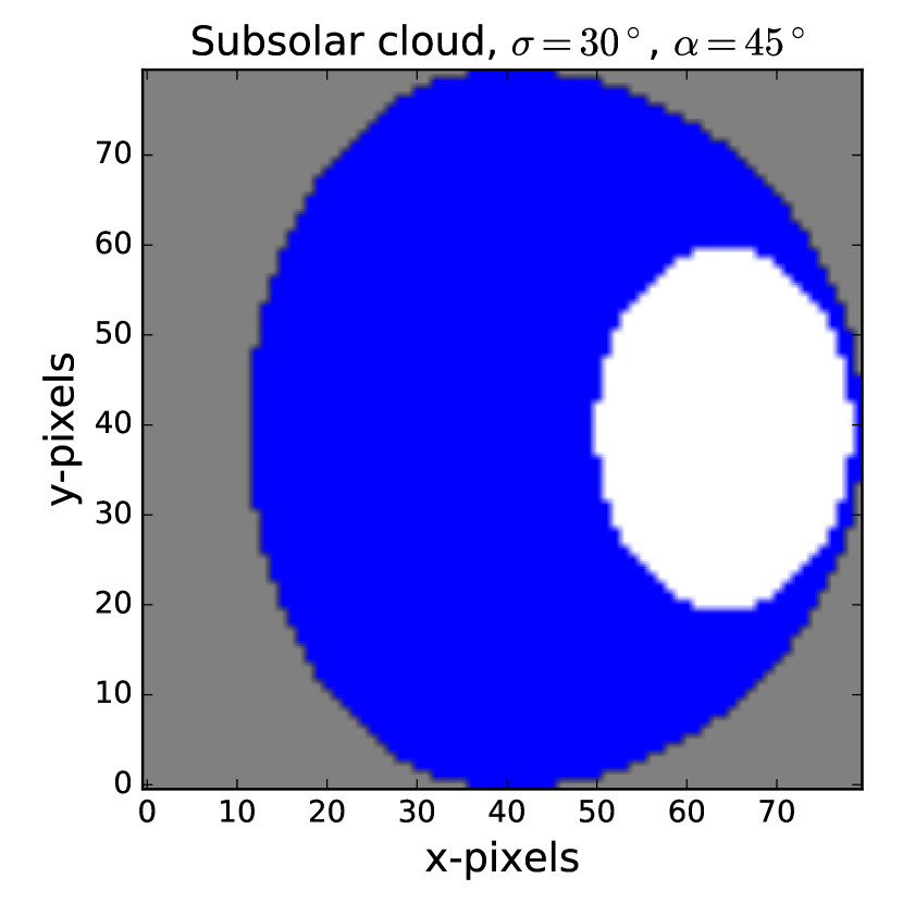
(a) A sub-solar cloud

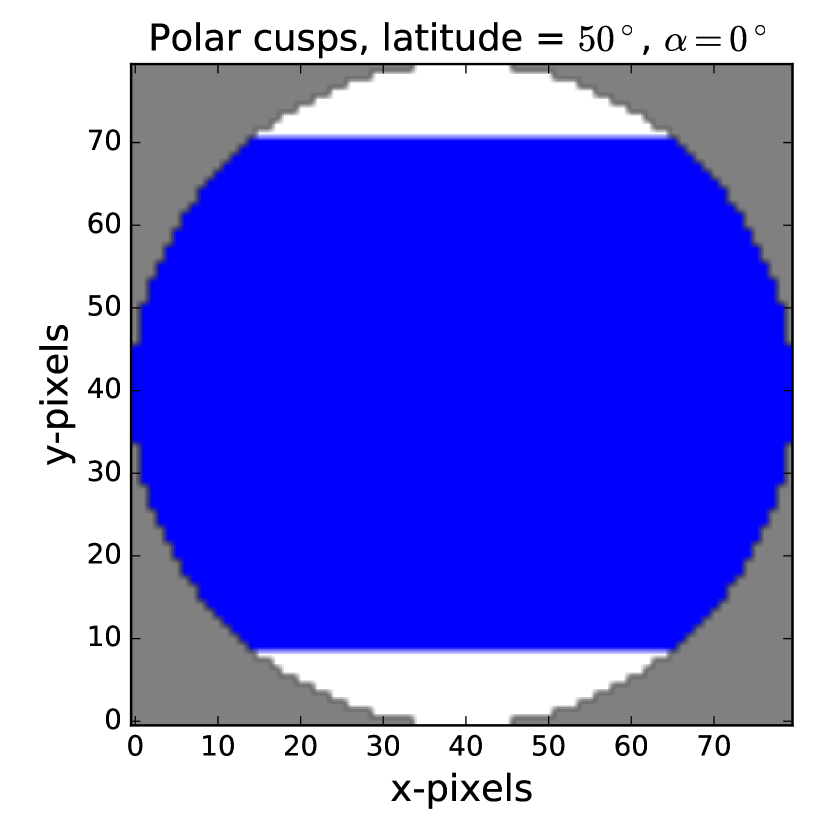
(b) Polar cusps

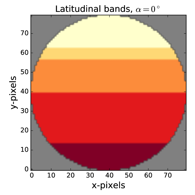
(c) Latitudinal bands

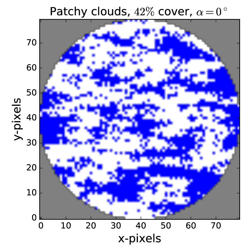
(d) Patchy clouds

Figure 5: Examples of four types of cloud cover: (a) Sub-solar clouds with an angular width $\sigma_{\rm c}$ of $30^{\circ}$ at $\alpha=45^{\circ}$; (b) Polar cusps for a threshold latitude $L_{\rm t}$ of 50^∘ at $\alpha=0^{\circ}$; (c) Latitudinal bands with borders at $-90^{\circ}$, $-40^{\circ}$, $0^{\circ}$, $25^{\circ}$, and $35^{\circ}$, $90^{\circ}$; (d) Patchy clouds for a cloud fraction $F_{\rm c}=0.42$ at $\alpha=0^{\circ}$. In all figures, $N_{\rm eq}=80$.

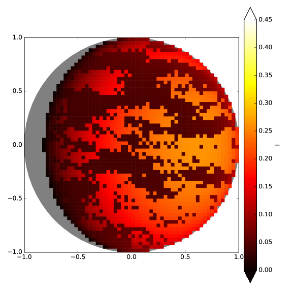
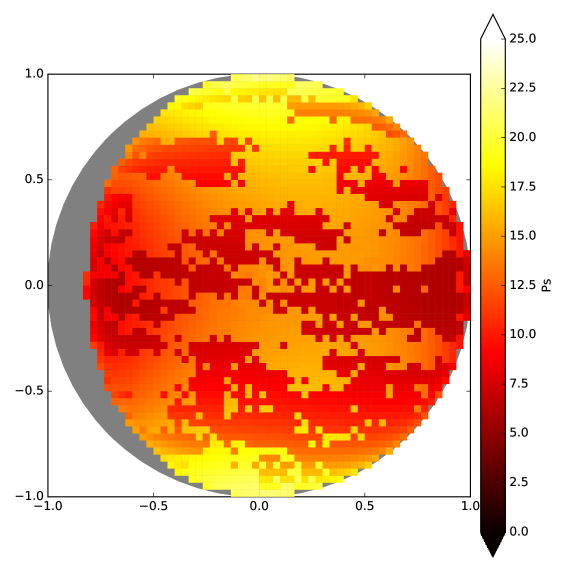
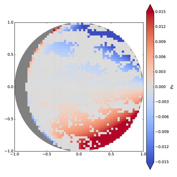
Figure 6: Computed disk–resolved locally reflected fluxes $I$ (top), $P_{\rm s}$ (middle, in percents) and $P_{\rm c}$ (bottom, in percents) at $\alpha=35^{\circ}$ and $\lambda=0.55\leavevmode\nobreak\ \mu$m, for a patchy cloud cover with $F_{\rm c}=0.50$. The cloud–free pixels have a pure gaseous (CO₂) model atmosphere with $b=7.0$. The cloudy pixels contain aerosol as described by Stam et al. (2006) (we let the model D type aerosol pose as cloud particles). The disk–integrated values are $F=0.32$, $P_{\rm s}=0.10$, and $P_{\rm c}=1.6\cdot 10^{-5}$. For all figures, $N_{eq}=60$.

The disk–integrated signal of a planet covered by patchy clouds will depend on the position of the cloudy pixels on the disk. To capture this variability, the user can choose to draw several patterns randomly at each phase angle. PyMieDAP will return the average and standard deviations of the values of $I$, $Q$, $U$, and $V$ over all patterns. It can also store the values for each pattern, providing the user insight into the variability.

An example of the variability computed using PyMieDAP can be found in Rossi & Stam (2017) where it was used to generate the disk–integrated signals of Earth–like exoplanets with varying types and amount of coverage by liquid water clouds. Thanks to the use of Fourier coefficients, only a limited number of model computations were necessary: clear sky and cloudy case with different cloud–top altitudes. Furthermore, because the Fourier files allow for computation of the reflected Stokes vector of light for any geometry, it was possible to generate the Stokes vector of each pixel for the clear and cloudy cases, and then apply masks on these grids of pixels to obtain the desired cloud pattern. The variability due to patchy cloud cover could be simulated by simply using 300 patterns that were averaged.

Another example of use of patchy cloud masks in PyMieDAP can be found in Fauchez et al. (2017) where disk–integrated signals of exoplanets with patchy clouds were computed to investigate the effect of such clouds on the spectral signature of the O₂ A-absorption band in the flux and polarization of reflected starlight.

7 Benchmark results

Here, we will compare results of PyMieDAP against (published) results obtained with other codes. This comparison allows an assessment of the accuracy of PyMieDAP’s approach using computed Fourier coefficients files, and our results allow PyMieDAP users to check their PyMieDAP installation and understanding of the input and output files.

7.1 Locally reflected light

We compare our results for locally reflected light with those presented in Tables 5, 6, 9 and 10 of de Haan et al. (1987). We use the same adding-doubling algorithm as de Haan et al. (1987), with the same accuracy, i.e. 10^-6. However, while de Haan et al. (1987) compute the reflected Stokes vectors at precisely the specified values of $\theta_{0}$ and $\theta$, we use a Fourier coefficients file (with $\theta=\theta_{0}=0^{\circ}$ as supplemented Gaussian abscissae), combined with spline interpolation Press et al. (with the algorithm from 1992) to obtain the reflected Stokes vectors at the same geometries.

Two model atmosphere-surface combinations are considered in de Haan et al. (1987): model 1, with a single layer atmosphere containing only haze droplets, bounded below by a black surface, and model 2, with an upper atmospheric layer containing only gas and a second, lower layer containing a mixture of gas and haze droplets, bounded below by a Lambertian reflecting surface with albedo $A_{\rm s}$ of 0.1. The molecular depolarization factor $\rho$ is 0.0279. The haze particles in both atmospheres are water–haze L particles (Deirmendjian, 1969), with their optical properties calculated at $\lambda=0.7\leavevmode\nobreak\ \mu$m (for the single scattering expansion coefficients, see de Rooij & van der Stap, 1984). For model 1, $b^{\rm a}=b^{\rm a}_{\rm sca}=1.0$. For model 2, $b^{\rm m}=b^{\rm m}_{\rm sca}=0.1$ in each layer, and in the lower layer, $b^{\rm a}=b^{\rm a}_{\rm sca}=0.4$. The incident flux $\pi F_{0}$ equals $\pi$ ($F_{0}$ is thus 1.0).

Table 1 shows the Stokes vector elements of the locally reflected light for model 1 from de Haan et al. (1987) and calculated using PyMieDAP and 40 Gaussian abscissae ($N_{\rm G}=40$). Table 2 shows the results for model 2. As can be seen, PyMieDAP’s pre-calculated Fourier coefficients combined with spline interpolation yields accurate results for both models. Note that when $\mu=1.0$, i.e. the supplemented Gaussian abscissa in our Fourier files (cf. Sect. 5.2), we only have to interpolation between Fourier coefficients for $\mu_{0}$, not for $\mu$.

7.2 Disk-integrated reflected starlight

There are no disk–integrated Stokes parameters in de Haan et al. (1987). We therefore first compare the disk–integrated reflected total flux as computed using PyMieDAP against the analytical expression for the phase function of a Lambertian reflecting, spherical planet with a surface albedo $a_{\rm s}$, i.e. (see van de Hulst, 1980)

$$\psi(\alpha)=\frac{2}{3\pi}a_{\rm s}\left(\sin\alpha+\pi\cos\alpha-\alpha\cos\alpha\right).$$ (39)

Figure 7 shows $\psi$ calculated using PyMieDAP and $a_{\rm s}=1.0$. For $N_{\rm G}\geq 20$, these results are indistinguishable from those computed by Eq. 39. This comparison also shows the validity of calculating reflected disk–integrated fluxes under the assumption of a locally plane–parallel atmosphere and/or surface.

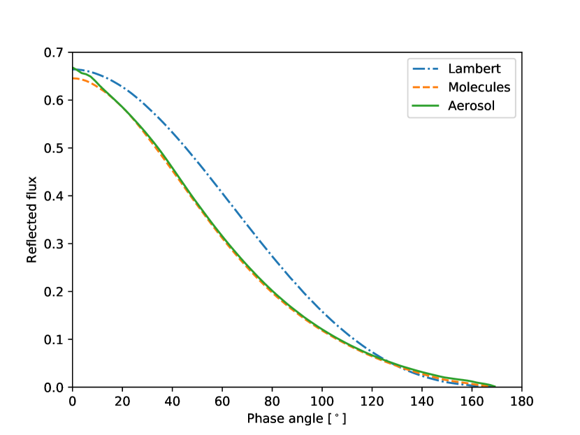
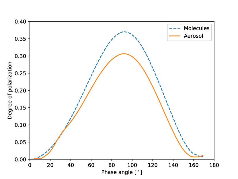
Figure 7: Numerical simulations of disk–integrated reflected fluxes (top) and the degree of linear polarization (bottom) as functions of $\alpha$ for different model planets. The flux curves are normalized such that they equal the planet’s geometric albedo $A_{\rm G}$ at $\alpha=0^{\circ}$. For all curves, $N_{eq}=20$. Dot-dashed line (only flux): a Lambertian reflecting planet with a surface albedo $a_{\rm s}=1.0$. Dashed line: a planet with a gaseous atmosphere with $b_{\rm sca}^{\rm m}=5.75$, $\rho=0.02$, and $a_{\rm s}=0.0$. Solid line: the same planet with model D aerosol (see text) added.

To test the accuracy of the computed disk–integrated polarization, we compare PyMieDAP results against results for two Jupiter–like gas planets computed with the same Fourier expansion coefficients but an integration method that treats the whole planet as a single scattering particle (Stam et al., 2006) (the latter method is only applicable to horizontally homogeneous planets).

The first planet (Sect. 4.1 of Stam et al., 2006) has a purely gaseous atmosphere with $b^{\rm m}_{\rm sca}=5.75$ and $b^{\rm m}_{\rm abs}=0.0$, and $\rho=0.02$ (i.e. representative for H₂). The surface albedo $a_{\rm s}=0.0$. Figure 7 shows the disk–integrated reflected total flux and degree of linear polarization as functions of $\alpha$ at $\lambda=0.55\leavevmode\nobreak\ \mu$m. According to Stam et al. (2006), the geometric albedo $A_{\rm G}$ of this planet is 0.647 and the maximum degree of polarization 0.37 (this value is reached at $\alpha=93^{\circ}$ (note that Stam et al. (2006) use the scattering angle $\Theta$ rather than $\alpha$ ($\Theta=180.0-\alpha$). Table 3 shows both the results of Stam et al. (2006) (interpolated linearly to obtain the values at the listed phase angles) and the results from PyMieDAP . Comparing the results, it is clear that PyMieDAP is very accurate, even for a relatively small number of Gaussian abscissae (i.e. $N_{\rm G}=20$).

The second planet (Sect. 4.2 of Stam et al., 2006) has the same gaseous atmosphere and black surface as the first, but with aerosol particles added. The aerosol optical thickness $b^{\rm a}=3.25$, yielding a total atmospheric optical thickness $b$ of 9.0 (at $\lambda=0.55\leavevmode\nobreak\ \mu$m). The aerosol particles are well–mixed with the gas molecules, and have the microphysical properties of the model D particles of de Rooij & van der Stap (1984). The disk–integrated reflected flux and degree of linear polarization as functions of $\alpha$ computed with PyMieDAP are shown in Fig. 7. The geometric albedo $A_{\rm G}$ of this second planet is 0.669 according to Stam et al. (2006). Table 4 is similar to Table 3, except for the second planet. Because the single scattering scattering matrix elements of model D aerosol particles show significant angular structures, in particular in the forward and backward scattering directions, more Gaussian abscissae are needed (by both disk-integration methods) to achieve accurate results across the whole phase angle range; we used $N_{\rm G}=50$.

Stokes parameter $I$
$\mu_{0}$ $\mu$ $\phi-\phi_{0}$ de Haan et al. PyMieDAP 0.5 0.1 0.0 1.102690 1.102679 0.5 0.5 0.0 0.319430 0.319428 0.5 1.0 0.0 0.033033 0.033033 0.5 0.1 30.0 0.664140 0.664143 0.5 0.5 30.0 0.252090 0.252094 0.5 1.0 30.0 0.033033 0.033033 0.1 0.1 0.0 2.932140 2.932100 0.1 0.5 0.0 0.220540 0.220536 0.1 1.0 0.0 0.009287 0.009287 0.1 0.1 30.0 0.769100 0.769102 0.1 0.5 30.0 0.132828 0.132829 0.1 1.0 30.0 0.009287 0.009287

Stokes parameter $Q$
$\mu_{0}$ $\mu$ $\phi-\phi_{0}$ de Haan et al. PyMieDAP 0.5 0.1 0.0 0.004604 0.004604 0.5 0.5 0.0 -0.002881 -0.002880 0.5 1.0 0.0 -0.002979 -0.002979 0.5 0.1 30.0 0.000303 0.000303 0.5 0.5 30.0 -0.001444 -0.001443 0.5 1.0 30.0 -0.001489 -0.001489 0.1 0.1 0.0 0.009900 0.009900 0.1 0.5 0.0 0.000976 0.000977 0.1 1.0 0.0 -0.000815 -0.000815 0.1 0.1 30.0 -0.003758 -0.003758 0.1 0.5 30.0 0.000220 0.000220 0.1 1.0 30.0 -0.000408 -0.000408

Stokes parameter $U$
$\mu_{0}$ $\mu$ $\phi-\phi_{0}$ de Haan et al. PyMieDAP 0.5 0.1 0.0 0.000000 0.000000 0.5 0.5 0.0 0.000000 0.000000 0.5 1.0 0.0 0.000000 0.000000 0.5 0.1 30.0 -0.002770 -0.002770 0.5 0.5 30.0 -0.004141 -0.004141 0.5 1.0 30.0 -0.002580 -0.002580 0.1 0.1 0.0 0.000000 0.000000 0.1 0.5 0.0 0.000000 0.000000 0.1 1.0 0.0 0.000000 0.000000 0.1 0.1 30.0 0.003124 0.003124 0.1 0.5 30.0 -0.000525 -0.000525 0.1 1.0 30.0 -0.000706 -0.000706

Stokes parameter $V$
$\mu_{0}$ $\mu$ $\phi-\phi_{0}$ de Haan et al. PyMieDAP 0.5 0.1 0.0 0.000000 0.000000 0.5 0.5 0.0 0.000000 0.000000 0.5 1.0 0.0 0.000000 0.000000 0.5 0.1 30.0 0.000038 0.000039 0.5 0.5 30.0 0.000017 0.000018 0.5 1.0 30.0 0.000000 0.000000 0.1 0.1 0.0 0.000000 0.000000 0.1 0.5 0.0 0.000000 0.000000 0.1 1.0 0.0 0.000000 0.000000 0.1 0.1 30.0 0.000012 0.000012 0.1 0.5 30.0 0.000007 0.000007 0.1 1.0 30.0 0.000000 0.000000

Table 1: Stokes parameters $I$, $Q$, $U$, and $V$ of the locally reflected light for model 1 (see Sect. 7.1) (a 1–layer atmosphere with water-haze L-aerosol and a black surface), as listed in Table 5 of de Haan et al. (1987), and as calculated using PyMieDAP with 40 Gaussian abscissae.

Stokes parameter $I$
$\mu_{0}$ $\mu$ $\phi-\phi_{0}$ de Haan et al. PyMieDAP 0.5 0.1 0.0 0.532950 0.532930 0.5 0.5 0.0 0.208430 0.208422 0.5 1.0 0.0 0.093680 0.093680 0.5 0.1 30.0 0.418140 0.418131 0.5 0.5 30.0 0.184970 0.184974 0.5 1.0 30.0 0.093680 0.093680 0.1 0.1 0.0 0.522770 0.522887 0.1 0.5 0.0 0.106590 0.106586 0.1 1.0 0.0 0.026009 0.026009 0.1 0.1 30.0 0.276300 0.276338 0.1 0.5 30.0 0.083628 0.083626 0.1 1.0 30.0 0.026009 0.026009

Stokes parameter $Q$
$\mu_{0}$ $\mu$ $\phi-\phi_{0}$ de Haan et al. PyMieDAP 0.5 0.1 0.0 -0.028340 -0.028339 0.5 0.5 0.0 -0.036299 -0.036298 0.5 1.0 0.0 -0.024156 -0.024156 0.5 0.1 30.0 -0.000058 -0.000057 0.5 0.5 30.0 -0.019649 -0.019649 0.5 1.0 30.0 -0.012078 -0.012078 0.1 0.1 0.0 0.011506 0.011509 0.1 0.5 0.0 -0.005186 -0.005185 0.1 1.0 0.0 -0.014984 -0.014984 0.1 0.1 30.0 0.034368 0.034376 0.1 0.5 30.0 0.003839 0.003840 0.1 1.0 30.0 -0.007492 -0.007492

Stokes parameter $U$
$\mu_{0}$ $\mu$ $\phi-\phi_{0}$ de Haan et al., PyMieDAP 0.5 0.1 0.0 0.000000 0.000000 0.5 0.5 0.0 0.000000 0.000000 0.5 1.0 0.0 0.000000 0.000000 0.5 0.1 30.0 -0.073105 -0.073105 0.5 0.5 30.0 -0.041401 -0.041401 0.5 1.0 30.0 -0.020920 -0.020919 0.1 0.1 0.0 0.000000 0.000000 0.1 0.5 0.0 0.000000 0.000000 0.1 1.0 0.0 0.000000 0.000000 0.1 0.1 30.0 -0.016042 -0.016043 0.1 0.5 30.0 -0.014492 -0.014492 0.1 1.0 30.0 -0.012976 -0.012976

Stokes parameter $V$
$\mu_{0}$ $\mu$ $\phi-\phi_{0}$ de Haan et al. PyMieDAP 0.5 0.1 0.0 0.000000 0.000000 0.5 0.5 0.0 0.000000 0.000000 0.5 1.0 0.0 0.000000 0.000000 0.5 0.1 30.0 0.000106 0.000101 0.5 0.5 30.0 0.000040 0.000036 0.5 1.0 30.0 0.000000 0.000000 0.1 0.1 0.0 0.000000 0.000000 0.1 0.5 0.0 0.000000 0.000000 0.1 1.0 0.0 0.000000 0.000000 0.1 0.1 30.0 0.000027 0.000027 0.1 0.5 30.0 0.000017 0.000017 0.1 1.0 30.0 0.000000 0.000000

Table 2: Similar to Table 1, except for model 2 (see Sect. 7.1) (a 2–layer atmosphere with gas and water-haze L-aerosol, and a surface with albedo 0.1), as listed in Table 9 of de Haan et al. (1987) and as calculated using PyMieDAP with 40 Gaussian abscissae.

$\alpha$	$F$		$P_{\rm s}$
	Stam et al.	PyMieDAP	Stam et al.	PyMieDAP
0.0	0.6471	0.6469	0.0000	0.0000
5.0	0.6424	0.6422	0.0021	0.0020
10.0	0.6299	0.6296	0.0081	0.0080
15.0	0.6108	0.6106	0.0179	0.0179
20.0	0.5861	0.5859	0.0315	0.0315
25.0	0.5570	0.5568	0.0487	0.0487
30.0	0.5245	0.5244	0.0693	0.0693
35.0	0.4898	0.4896	0.0930	0.0930
40.0	0.4536	0.4535	0.1195	0.1195
45.0	0.4171	0.4169	0.1483	0.1484
50.0	0.3808	0.3807	0.1789	0.1790
55.0	0.3455	0.3454	0.2105	0.2106
60.0	0.3118	0.3117	0.2422	0.2423
65.0	0.2799	0.2798	0.2730	0.2730
70.0	0.2501	0.2501	0.3015	0.3016
75.0	0.2226	0.2226	0.3266	0.3267
80.0	0.1975	0.1975	0.3469	0.3470
85.0	0.1745	0.1746	0.3613	0.3614
90.0	0.1537	0.1538	0.3689	0.3690
95.0	0.1349	0.1350	0.3690	0.3691
100.0	0.1179	0.1179	0.3615	0.3616
105.0	0.1024	0.1025	0.3466	0.3466
110.0	0.0883	0.0884	0.3249	0.3250
115.0	0.0755	0.0756	0.2976	0.2977
120.0	0.0638	0.0639	0.2659	0.2659
125.0	0.0531	0.0532	0.2311	0.2311
130.0	0.0434	0.0435	0.1946	0.1947
135.0	0.0347	0.0348	0.1579	0.1579
140.0	0.0269	0.0270	0.1220	0.1220
145.0	0.0201	0.0202	0.0882	0.0881
150.0	0.0143	0.0144	0.0573	0.0571
155.0	0.0095	0.0096	0.0302	0.0299
160.0	0.0058	0.0058	0.0079	0.0071
165.0	0.0031	0.0031	-0.0088	-0.0095
170.0	0.0012	0.0012	-0.0184	-0.0221
175.0	0.0003	0.0002	-0.0186	-0.0270
180.0	0.0000	0.0000	0.0000	0.0000

Table 3: The flux and degree of polarization of light that is reflected by a planet with a gaseous atmosphere with $b=5.75$, bounded below by a black surface, as a function of $\alpha$, as computed by Stam et al. (2006) and by using PyMieDAP . The number of Gaussian abscissae, $N_{\rm G}$, is 20 and $N_{\rm eq}=100$. The fluxes have been normalized such that $F(0^{\circ})=A_{\rm G}$.

$\alpha$	$F$		$P_{\rm s}$
	Stam et al.	PyMieDAP	Stam et al.	PyMieDAP
0.0	0.6688	0.6676	0.0000	0.0000
5.0	0.6512	0.6542	0.0023	-0.0000
10.0	0.6439	0.6361	-0.0047	-0.0003
15.0	0.6128	0.6113	0.0083	0.0095
20.0	0.5866	0.5857	0.0272	0.0229
25.0	0.5593	0.5580	0.0496	0.0462
30.0	0.5294	0.5288	0.0691	0.0710
35.0	0.4956	0.4957	0.0860	0.0901
40.0	0.4590	0.4589	0.1040	0.1077
45.0	0.4215	0.4212	0.1253	0.1285
50.0	0.3849	0.3844	0.1494	0.1527
55.0	0.3497	0.3492	0.1749	0.1784
60.0	0.3163	0.3157	0.2005	0.2043
65.0	0.2847	0.2841	0.2251	0.2292
70.0	0.2550	0.2545	0.2475	0.2519
75.0	0.2275	0.2269	0.2669	0.2716
80.0	0.2020	0.2015	0.2824	0.2874
85.0	0.1787	0.1782	0.2932	0.2985
90.0	0.1575	0.1571	0.2986	0.3042
95.0	0.1382	0.1378	0.2980	0.3037
100.0	0.1208	0.1204	0.2912	0.2968
105.0	0.1050	0.1047	0.2782	0.2836
110.0	0.0907	0.0905	0.2593	0.2643
115.0	0.0778	0.0776	0.2353	0.2397
120.0	0.0662	0.0661	0.2073	0.2111
125.0	0.0557	0.0557	0.1765	0.1794
130.0	0.0463	0.0464	0.1444	0.1461
135.0	0.0380	0.0381	0.1126	0.1132
140.0	0.0306	0.0309	0.0827	0.0816
145.0	0.0242	0.0246	0.0561	0.0530
150.0	0.0187	0.0192	0.0340	0.0293
155.0	0.0140	0.0144	0.0171	0.0125
160.0	0.0101	0.0103	0.0061	0.0031
165.0	0.0068	0.0069	0.0017	0.0006
170.0	0.0045	0.0039	-0.0037	0.0019
175.0	0.0054	0.0032	-0.0042	-0.0043
180.0	0.0000	0.0000	0.0000	0.0000

Table 4: Similar to Table 3, except for a model atmosphere with model D aerosol (de Rooij & van der Stap, 1984) added, such that $b=9.0$. For these computations, $N_{\rm G}=50$.

8 Summary

We presented PyMieDAP, a modular Python–based tool to compute the total and polarized fluxes of light that is reflected by (exo)planets (or moons) with locally horizontally homogeneous, plane–parallel atmospheres bounded below by a horizontally homogeneous, flat surface. The atmospheres can be vertically inhomogeneous. Horizontally inhomogeneous planets are modelled by assigning different atmosphere-surface combinations to different regions on the planet. The Fortran radiative transfer algorithm is based on the adding–doubling method as described by de Haan et al. (1987), and fully includes linear and circular polarization for all orders of scattering. The single scattering of light by atmospheric aerosols is computed using Mie–scattering, based on de Rooij & van der Stap (1984).

PyMieDAP has a two-step approach: first, the adding–doubling radiative transfer computations provide files with Fourier coefficients of the expansion of the local reflection matrix of the model planetary atmosphere and surface, and, second, the Fourier coefficients are used to efficiently compute the locally reflected Stokes vectors for every given geometry. The latter Stokes parameters can be summed up to provide the disk–integrated Stokes parameters of the reflected starlight. By storing the Fourier–coefficient files for later use, significant amounts of computing time can be saved in the computation of the reflected light vectors.

The modular aspect of PyMieDAP allows users to define an atmosphere-surface model and to compute spatially resolved and/or disk–integrated signals of a planet at a range of phase angle in a single function call. PyMieDAP can straightforwardly be used to model signals of horizontally inhomogeneous planets by assigning different atmosphere–surface models to different regions on a planet. Four pre-defined cloud types or ’masks’ are included in the code. The modular aspect of the code also allows for step-by-step computations, for users who wish to perform more complicated cases.

PyMieDAP is distributed under the GNU GPL license and we invite interested users to suggest improvements or extensions to broaden the application of the code.

Acknowledgements

L.R. acknowledges the support of the Dutch Scientific Organization (NWO) through the PEPSci network of planetary and exoplanetary science. The authors thank Gourav Mahapatra and Ashwyn Groot, who were kind enough to test the code before its public release.

Appendix A Fourier file formats

A Fourier–coefficients file for a given model atmosphere-surface combination has the following format:

The first lines contain comments, including a reference, and they have details on the model atmosphere and surface. The number of these lines depends on the number of layers in the model atmosphere, but they are all preceded by a ’#’. In the following, we will assume the number of comment lines is $N$.

Line $N+1$ contains a number to describe the size of the reflected light vectors: ’1’ indicates only $I$, ’3’ indicates $I$, $Q$, and $U$, and ’4’ indicates $I$, $Q$, $U$, and $V$.

Line $N+2$ contains the number of Gaussian abscissae $G$ plus the supplemented value 1.0. It thus contains the value $G+1$.

Lines $N+3$ up to and including $N+4+N_{\rm G}$ contain the $N_{\rm G}$ Gaussian abscissae (the cosines of the corresponding illumination and viewing zenith angles) plus the supplemented value 1.0, and the corresponding Gaussian weights. For the supplemented value, this weight is set equal to 1.0.

Starting with line $N+N_{\rm G}+5$, the elements of the first column of the local reflection matrix ${\bf R}$, i.e. $R^{m}_{11}$, $R^{m}_{21}$, $R^{m}_{31}$, and $R^{m}_{41}$ (see Eqs. 34-37) are listed, with $m$ the number of the Fourier term ($0\leq m\leq M$, with $M$ the number of the last Fourier term). Elements $R^{m}_{21}$ and $R^{m}_{31}$ are only listed if the polarized fluxes have actually been calculated, and element $R^{m}_{41}$ is only listed if the circularly polarized flux has also been calculated. The matrix elements depend not only on the number of the Fourier term, $m$, but also on the illumination and viewing zenith angles, i.e. on $\mu$ and $\mu_{0}$. With $N_{\rm G}$ ’true’ Gaussian abscissae and 1 supplemented value, we have $(N_{\rm G}+1)^{2}$ combinations of $\mu$ and $\mu_{0}$.

Each line has the format: $m$, $i$, $j$, $R^{m}_{k1}$, with $k$ equal to 1, 3, or 4, with $i$ the number of the Gaussian abscissae representing $\mu$ ($1\leq i\leq N_{\rm G}+1$), and with $j$ the number of the Gaussian abscissae representing $\mu_{0}$ ($1\leq j\leq N_{\rm G}+1$). Each file thus has $(M+1)(N_{\rm G}+1)^{2}$ lines with 1 to 4 elements of the first column of the local reflection matrix ${\bf R}$. For a purely gaseous atmosphere, $M=2$, and given $N_{\rm G}=20$, the total number of lines with matrix elements is thus 1,323. Model atmospheres with aerosol and/or cloud particles will usually require much larger values for $M$, and will thus yield much larger data files.

Appendix B Computation of the local angles

We describe here equations that are used to compute the local illumination and viewing angles $\theta_{0i}$, $\theta_{i}$, $\beta_{i}$ and $\phi_{i}-\phi_{0i}$ for a pixel $i$ in the pixel grid. First, we define the planetocentric reference frame $(\mathbf{u_{x}},\mathbf{u_{y}},\mathbf{u_{z}})$, where $\mathbf{u_{x}}$ and $\mathbf{u_{y}}$ lie in the plane of the observer’s sky, while $\mathbf{u_{z}}$ points towards the observer.

Assume that the coordinates of pixel $i$ in the plane of the sky are given by $(x_{i},y_{i})$. Assuming that the planet is spherical with a radius equal to one, we know that the 3D coordinates of the projected pixel centre on the planet are $(x_{i},y_{i},z_{i})$ with $z_{i}=(x_{i}^{2}+y_{i}^{2})^{1/2}$.

The local zenith direction for pixel $i$ is given by vector

$$\mathbf{r_{cp}}=\left[\begin{array}[]{c}x_{i}\\ y_{i}\\ z_{i}\end{array}\right],$$ (40)

and the vector pointing to the star is given by

$$\mathbf{r_{cs}}=\left[\begin{array}[]{c}\sin{\alpha}\\ 0\\ \cos{\alpha}\end{array}\right],$$ (41)

where $\alpha$ is the planetary phase angle, i.e. the angle between the direction to the observer and the direction to the star as measured from the centre of the planet. The local solar/stellar zenith angle is thus given by

$$\theta_{0i}=\mathbf{r_{cp}}\cdot\mathbf{r_{cs}}=\arccos(x_{i}\sin{\alpha}+z_{i}\cos{\alpha}),$$ (42)

and, since unit vector $\mathbf{u_{z}}$ is pointing towards the observer, the local viewing zenith angle is given by

$$\theta_{i}=\arccos{z_{i}}.$$ (43)

The local azimuthal difference angle $\phi_{i}-\phi_{0i}$ can be computed using the spherical law of cosines:

$$\cos{\alpha}=\cos{\theta_{0i}}\cos{\theta_{i}}+\sin{\theta_{0i}}\sin{\theta_{i}}\cos(\phi_{i}-\phi_{0i}),$$ (44)

and thus

$$\phi_{i}-\phi_{0i}=\arccos\left(\frac{\cos{\alpha}-\cos{\theta_{0i}}\cos{\theta_{i}}}{\sin{\theta_{0i}}\sin{\theta_{i}}}\right).$$ (45)

For $0<\alpha<\pi$, the local rotation angle $\beta_{i}$ that is used to rotate computed Stokes parameters defined with respect to the local meridian planet to the planetary scattering plane is given by

$$\beta_{i}=\begin{cases}\arctan{\left(y_{i}/x_{i}\right)}&\mathrm{if}\hskip 5.69046ptx_{i}\hskip 1.42271pty_{i}\geq 0\\ 180^{\circ}+\arctan{\left(y_{i}/x_{i}\right)}&\mathrm{if}\hskip 5.69046ptx_{i}\hskip 1.42271pty_{i}<0\\ \end{cases}$$ (46)

For $\pi<\alpha<2\pi$, rotation angle $\beta_{i}$ is given by

$$\beta_{i}=\begin{cases}180^{\circ}-\arctan{\left(y_{i}/x_{i}\right)}&\mathrm{if}\hskip 5.69046ptx_{i}\hskip 1.42271pty_{i}\geq 0\\ -\arctan{\left(y_{i}/x_{i}\right)}&\mathrm{if}\hskip 5.69046ptx_{i}\hskip 1.42271pty_{i}<0\\ \end{cases}$$ (47)

References

- Aben et al. (1997) Aben, I., Helderman, F., Stam, D., & Stammes, P. 1997, in Polarization: Measurement, Analysis, and Remote Sensing. Proceedings SPIE 3121, ed. D. Goldstein & R. Chipman, 446–451
- Bates (1984) Bates, D. R. 1984, Planet. Space Sci., 32, 785
- Bideau-Mehu et al. (1973) Bideau-Mehu, A., Guern, Y., Abjean, R., & Johannin-Gilles, A. 1973, Optics Communications, 9, 432
- Boesche et al. (2009) Boesche, E., Stammes, P., & Bennartz, R. 2009, Journal of Quantitative Spectroscopy and Radiative Transfer, 110, 223
- Bohren & Huffman (1983) Bohren, C. & Huffman, D. 1983, Absorption and scattering of light by small particles (Wiley), 477–482
- Ciddor (1996) Ciddor, P. E. 1996, Applied optics, 35, 1566
- Cotton et al. (2017) Cotton, D. V., Marshall, J. P., Bailey, J., et al. 2017, Monthly Notices of the Royal Astronomical Society, 467, 873
- de Haan et al. (1987) de Haan, J. F., Bosma, P. B., & Hovenier, J. W. 1987, A&A, 183, 371
- de Rooij & van der Stap (1984) de Rooij, W. A. & van der Stap, C. C. A. H. 1984, A&A, 131, 237
- Deirmendjian (1969) Deirmendjian, D. 1969, Electromagnetic scattering on spherical polydispersions.
- Fauchez et al. (2017) Fauchez, T., Rossi, L., & Stam, D. M. 2017, The Astrophysical Journal, 842, 41
- Grainger & Ring (1962) Grainger, J. F. & Ring, J. 1962, Nature, 193, 762
- Hansen & Hovenier (1974) Hansen, J. E. & Hovenier, J. W. 1974, Journal of Atmospheric Sciences, 31, 1137
- Hansen & Travis (1974) Hansen, J. E. & Travis, L. D. 1974, Space Science Reviews, 16, 527
- Hovenier & Stam (2005) Hovenier, J. W. & Stam, D. M. 2005, Journal of Quantitative Spectroscopy and Radiative Transfer (in press)
- Hovenier et al. (2004) Hovenier, J. W., van der Mee, C., & Domke, H. 2004, Transfer of Polarized Light in Planetary Atmospheres; Basic Concepts and Practical Methods (Kluwer, Dordrecht; Springer, Berlin)
- Hovenier & van der Mee (1983) Hovenier, J. W. & van der Mee, C. V. M. 1983, A&A, 128, 1
- Kemp et al. (1987) Kemp, J. C., Henson, G. D., Steiner, C. T., & Powell, E. R. 1987, Nature, 326, 270
- Mansfield & Peck (1969) Mansfield, C. R. & Peck, E. R. 1969, JOSA, 59, 199
- Mishchenko et al. (1994) Mishchenko, M. I., Lacis, A. A., & Travis, L. D. 1994, Journal of Quantitative Spectroscopy and Radiative Transfer, 51, 491
- Mishchenko et al. (2002) Mishchenko, M. I., Travis, L. D., & Lacis, A. A. 2002, Scattering, absorption, and emission of light by small particles
- Muñoz et al. (2012) Muñoz, O., Moreno, F., Guirado, D., et al. 2012, J. Quant. Spec. Radiat. Transf., 113, 565
- Peck & Huang (1977) Peck, E. R. & Huang, S. 1977, JOSA, 67, 1550
- Peck & Khanna (1966) Peck, E. R. & Khanna, B. N. 1966, JOSA, 56, 1059
- Peterson (2009) Peterson, P. 2009, International Journal of Computational Science and Engineering, 4, 296
- Pierrehumbert (2011) Pierrehumbert, R. T. 2011, The Astrophysical Journal Letters, 726, L8
- Press et al. (1992) Press, W. H., Teukolsky, S. A., Vetterling, W. T., & Flannery, B. P. 1992, Numerical recipes in FORTRAN. The art of scientific computing
- Rossi & Stam (2017) Rossi, L. & Stam, D. 2017, Astronomy & Astrophysics
- Seager et al. (2000) Seager, S., Whitney, B. A., & Sasselov, D. D. 2000, ApJ, 540, 504
- Sneep & Ubachs (2005) Sneep, M. & Ubachs, W. 2005, J. Quant. Spec. Radiat. Transf., 92, 293
- Stam (2008) Stam, D. M. 2008, A&A, 482, 989
- Stam et al. (2002) Stam, D. M., Aben, I., & Helderman, F. 2002, Journal of Geophysical Research (Atmospheres), AAC 1
- Stam et al. (2000) Stam, D. M., De Haan, J. F., Hovenier, J. W., & Aben, I. 2000, J. Geophys. Res., 22379
- Stam et al. (2006) Stam, D. M., de Rooij, W. A., Cornet, G., & Hovenier, J. W. 2006, A&A, 452, 669
- Stam & Hovenier (2005) Stam, D. M. & Hovenier, J. W. 2005, A&A, 444, 275
- Stam et al. (2004) Stam, D. M., Hovenier, J. W., & Waters, L. B. F. M. 2004, A&A, 428, 663
- Stammes et al. (1994) Stammes, P., Kuik, F., & de Haan, J. 1994, in Proceedings PIERS 1994, Kluwer Acad., Dordrecht, ed. B. e. a. Arbesser-Rastburg, 2255–2259
- Turbet et al. (2016) Turbet, M., Leconte, J., Selsis, F., et al. 2016, A&A, 596, A112
- van de Hulst (1980) van de Hulst, H. C. 1980, Multiple Light Scattering, Tables, Formulas, and Applications, Vols. 1 and 2 (Academic Press, New York.)
- Yang et al. (2013) Yang, J., Cowan, N. B., & Abbot, D. S. 2013, The Astrophysical Journal Letters, 771, L45
- Young (1981) Young, A. T. 1981, Appl. Opt., 20, 533
- Yurkin & Hoekstra (2011) Yurkin, M. A. & Hoekstra, A. G. 2011, J. Quant. Spec. Radiat. Transf., 112, 2234