Optimal Transport Approximation of 2-Dimensional Measures

Abstract

We propose a fast and scalable algorithm to project a given density on a set of structured measures defined over a compact 2D domain. The measures can be discrete or supported on curves for instance. The proposed principle and algorithm are a natural generalization of previous results revolving around the generation of blue-noise point distributions, such as Lloyd’s algorithm or more advanced techniques based on power diagrams. We analyze the convergence properties and propose new approaches to accelerate the generation of point distributions. We also design new algorithms to project curves onto spaces of curves with bounded length and curvature or speed and acceleration. We illustrate the algorithm’s interest through applications in advanced sampling theory, non-photorealistic rendering and path planning.

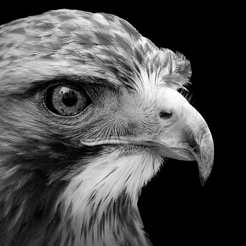
(a) Original

(b) Stippling

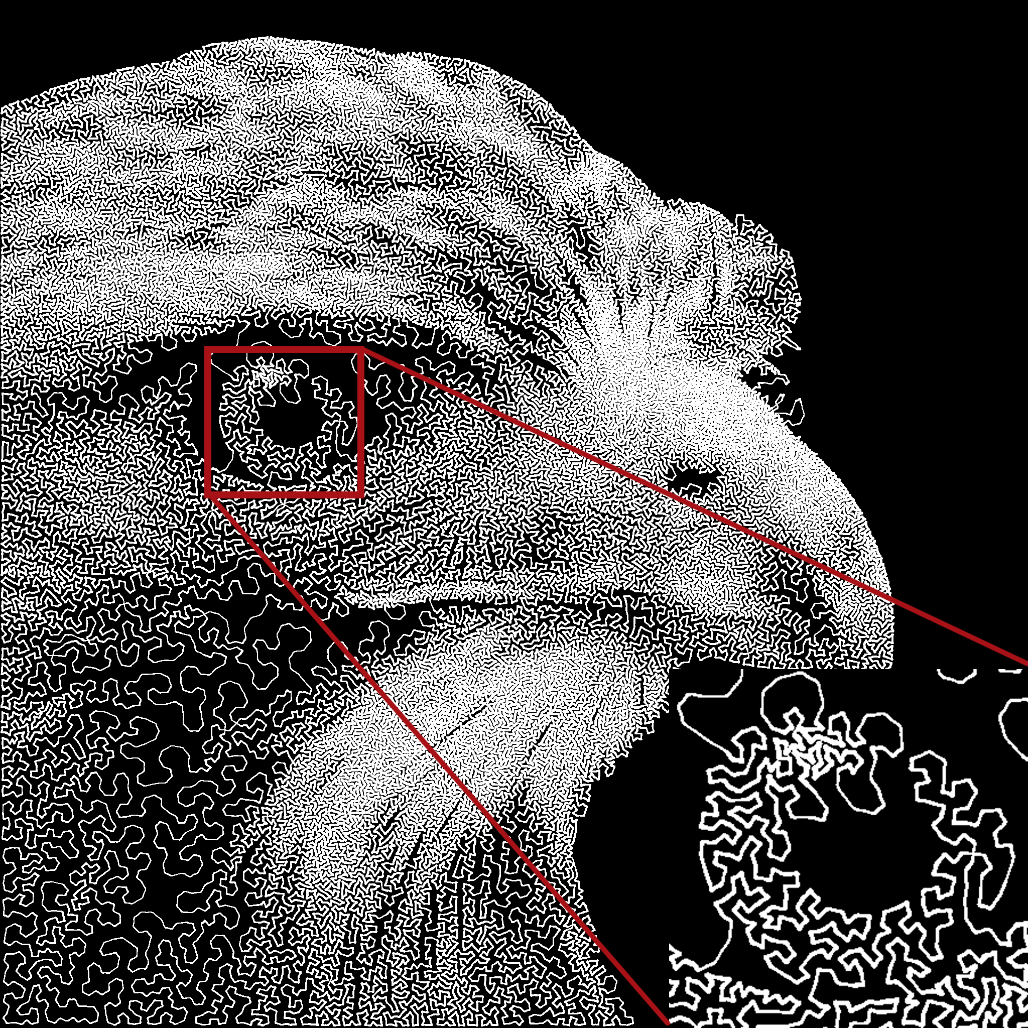
(c) Curvling

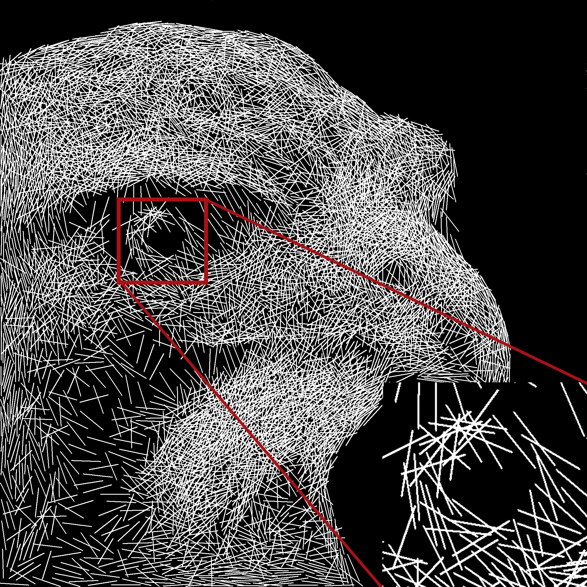
(d) Dashing

Figure 1: Approximating an image with a measure supported on points (stippling, 100k, 202”), curve (curvling, 100k, 313”) or segments (dashing, 33k, 237”). In each case, the iterative algorithm starts from a set of points drawn uniformly at random.

1 Introduction

The aim of this paper is to approximate a target measure $\mu$ with probability density function $\rho:\Omega\to\mathbb{R}_{+}$ with probability measures possessing some structure. This problem arises in a large variety of fields including finance [47], computer graphics [53], sampling theory [7] or optimal facility location [23]. An example in non photo-realistic rendering is shown in Figure 1, where the target image in Fig. 1a is approximated by an atomic measure in Fig. 1b, by a smooth curve in Fig. 1c and by a set of segments in Fig. 1d. Given a set of admissible measures $\mathcal{M}$ (i.e. atomic measures, measures supported on smooth curves or segments), the best approximation problem can be expressed as follows:

$$\min_{\nu\in\mathcal{M}}D(\nu,\mu),$$ (1)

where $D$ is a distance between measures.

1.1 Contributions

Our main contributions in this article are listed below.

• Develop a few original applications for the proposed algorithm.

• Develop a fast numerical algorithm to minimize problem (1), when $D$ is the $W_{2}$ transportation distance and $\Omega=[0,1]^{2}$.

• Show its connections to existing methods such as Lloyd’s algorithm [38] or optimal transport halftoning [15].

• Provide some theoretical convergence guarantees for the computation of the optimal semi-discrete transportation plan, especially for complicated point configurations and densities, for which an analysis was still lacking.

• Design algorithms specific to the case where the space of admissible measures $\mathcal{M}$ consists of measures supported on curves with geometric constraints (e.g. fixed length and bounded curvature).

• Generate a gallery of results to show the versatility of the approach.

In the next section, we put our main contributions in perspective.

1.2 Related works

1.2.1 Projections on measure spaces

To the best of our knowledge, the generic problem (1) was first proposed in [10] with a distance $D$ constructed through a convolution kernel. Similar problems were considered earlier, with spaces of measures restricted to a fixed support for instance [39], but not with the same level of generality.

Formulation (1) covers a large amount of applications that are often not formulated explicitly as optimization problems. We review a few of them below.

Finitely supported measures

A lot of approaches have been developed when $\mathcal{M}$ is the set of uniform finitely supported measures

$$\mathcal{M}_{f,n}=\left\{\nu(\mathbf{x})=\frac{1}{n}\sum_{i=1}^{n}\delta_{\mathbf{x}[i]},\mathbf{x}\in\Omega^{n}\right\},$$ (2)

where $n$ is the support cardinality, or the set of atomic measures defined by:

$$\mathcal{M}_{a,n}\!\!=\!\left\{\nu(\mathbf{x},\mathbf{w})\!=\!\sum_{i=1}^{n}\!\!\mathbf{w}[i]\delta_{\mathbf{x}[i]},\mathbf{x}\in\Omega^{n},\mathbf{w}\in\Delta_{n-1}\right\}\!,$$ (3)

where $\Delta_{n-1}=\left\{\sum_{i=1}^{n}\mathbf{w}[i]=1,\mathbf{w}[i]\geq 0,\ \forall i\right\}$ is the canonical simplex.

For these finitely supported measure sets, solving problem (1) yields nice stippling results, which is the process of approximating an image with a finite set of dots (see Fig. 1b). This problem has a long history and a large amount of methods were designed to find dots locations and radii that minimize visual artifacts due to discretization [20, 38, 57, 6]. Lloyd’s algorithm is among the most popular. We will see later that this algorithm is a solver of (1), with $\mathcal{M}=\mathcal{M}_{a,n}$. Lately, explicit variational approaches [52, 15] have been developed. The work of The work of de Goes et al [15] is closely related to our paper since they propose solving (1), where $D$ is the $W_{2}$ transportation distance and $\mathcal{M}=\mathcal{M}_{f,n}$. This sole problem is by no means limited to stippling and it is hard to provide a comprehensive list of applications. A few of them are listed in the introduction of [62].

Best approximation with curves

Another problem that is met frequently is to approximate a density by a curve. This can be used for non photorealitistic rendering of images or sculptures [32, 2]. It can also be used to design trajectories of the nozzle of 3D printers [12]. It was also used for the generation of sampling schemes [7].

Apart from the last application, this problem is usually solved with methods that are not clearly expressed as an optimization problem.

Best approximation with arbitrary objects

Problem (1) encompasses many other applications such as the optimization of networks [23], texture rendering or non photorealistic rendering [28, 29, 51, 33, 17], or sampling theory [8].

Overall, this paper unifies many problems that are often considered as distinct with specific methods.

1.2.2 Numerical optimal transport

In order to quantify the distance between the two measures, we use transportation distances [43, 31, 58]. In our work, we are interested mostly in the semi-discrete setting, where one measure is a density and the other is discrete. In this setting, the most intuitive way to introduce this distance is via Monge’s transportation plan and allocation problems. Given an atomic measure $\nu\in\mathcal{M}_{{a,n}}$ and a measure $\mu$ with density, a transport plan $T\in\mathcal{T}(\mathbf{x},\mathbf{w})$ is a mapping $T:\Omega\to\{\mathbf{x}[1],\ldots,\mathbf{x}[n]\}$ such that $\forall 1\leq i\leq n,\mu(T^{-1}(\mathbf{x}[i]))=\mathbf{w}[i]$. In words, the mass at any point $x\in\Omega$ is transported to point $T(x)$. In this setting, the $W_{2}$ transportation distance is defined by:

$$W_{2}^{2}(\mu,\nu)=\inf_{T\in\mathcal{T}(\mathbf{x},\mathbf{w})}\int_{\Omega}\|x-T(x)\|_{2}^{2}d\mu(x),$$ (4)

and the minimizing mapping $T$ describes the optimal way to transfer $\mu$ to $\nu$.

Computing the transport plan $T$ and the distance $W_{2}$ is a challenging optimization problem. In the semi-discrete setting, the paper [5] provided an efficient method based on “power diagram” or “Laguerre diagram”. This framework was recently further improved and analyzed recently in [15, 40, 35, 34]. The idea is to optimize a concave cost function with second-order algorithms. We will make use of those results in the paper, and improve them by stabilizing them while keeping the second-order information.

1.2.3 Numerical projections on curve spaces

Projecting curves on admissible sets is a basic brick for many algorithms. For instance, mobile robots are subject to kinematic constraints (speed and acceleration), while steel wire sculptures have geometric constraints (length, curvature).

While the projection on kinematic constraints is quite easy, due to convexity of the underlying set [11], we believe that this is the first time projectors on sets defined through intrinsic geometry are designed. Similar ideas have been explored in the past. For instance, curve shortening with mean curvature motion [19] is a long-studied problem with multiple applications in computer graphics and image processing [63, 42, 54]. The proposed algorithms allow exploring new problems such as curve lengthening with curvature constraints.

1.3 Paper outline

The rest of the paper is organized as follows. We first outline the overarching algorithm in Section 2. In Sections 3 and 4, we describe more precisely and study the theoretical guarantees of the algorithms used respectively for computing the Wasserstein distance, and for optimising the positions and weights of the points. We describe the relationships with previous models in Section 5. The algorithms in Sections 3 and 4 are enough for, say, halftoning, but do not handle constraints on the points. In Section 6, we add those constraints and design algorithms to make projections onto curves spaces with bounded speed and acceleration, or bounded length and curvature. Finally some application examples and results are shown in Section 7.

2 The minimization framework

In this section, we show how to numerically solve the best approximation problem:

$$\inf_{\nu\in\mathcal{M}}W_{2}^{2}(\nu,\mu),$$ (5)

where $\mathcal{M}$ is an arbitrary set of measures supported on $\Omega=[0,1]^{2}$.

2.1 Discretization

Problem (5) is infinite-dimensional and first needs to be discretized to be solved using a computer. We propose to approximate $\mathcal{M}$ by a subset $\mathcal{M}_{n}\subseteq\mathcal{M}_{a,n}$ of the atomic measures with $n$ atoms. The idea is to construct $\mathcal{M}_{n}$ as

$$\mathcal{M}_{n}=\{\nu(\mathbf{x},\mathbf{w}),\mathbf{x}\in\mathbf{X}_{n},\mathbf{w}\in\mathbf{W}_{n}\},$$ (6)

where the mapping $\nu:(\Omega^{n}\times\Delta_{n-1})\to\mathcal{M}_{a,n}$ is defined by

$$\nu(\mathbf{x},\mathbf{w})=\sum_{i=1}^{n}\mathbf{w}[i]\delta_{\mathbf{x}[i]}.$$ (7)

The constraint set $\mathbf{X}_{n}\subseteq\Omega^{n}$ describes interactions between points and the set $\mathbf{W}_{n}\subseteq\Delta_{n-1}$ describes the admissible weights.

We have shown in [10] that for any subset $\mathcal{M}$ of the probability measures, it is possible to construct a sequence of approximation spaces $(\mathcal{M}_{n})_{n\in\mathbb{N}}$ of the type (6), such that the solution sequence $(\nu_{n}^{*})_{n\in\mathbb{N}}$ of the discretized problem

$$\inf_{\nu\in\mathcal{M}_{n}}W_{2}^{2}(\nu,\mu),$$ (8)

converges weakly along a subsequence to a global minimizer $\nu^{*}$ of the original problem (5). Let us give a simple example: assume that $\mathcal{M}$ is a set of pushforward measures of curves parameterized by a $1$-Lipchitz function on $[0,1]$. This curve can be discretized by a sum of $n$ Dirac masses with a distance between consecutive samples bounded by $1/n$. It can then be shown that this space $\mathcal{M}_{n}$ approximates $\mathcal{M}$ well, in the sense that each element of $\mathcal{M}_{n}$ can be approximated with a distance $O(1/n)$ by an element in $\mathcal{M}$ and vice-versa [10]. We will show explicit constructions of more complicated constraint sets $\mathbf{X}_{n}$ and $\mathbf{W}_{n}$ for measures supported on curves in Section 6.

The discretized problem (8) can now be rewritten in a form convenient for numerical optimization:

$$\min_{\mathbf{x}\in\mathbf{X},\mathbf{w}\in\mathbf{W}}F(\mathbf{x},\mathbf{w}),$$ (9)

where we dropped the index $n$ to simplify the presentation and where

$$F(\mathbf{x},\mathbf{w})=\frac{1}{2}W_{2}^{2}(\nu(\mathbf{x},\mathbf{w}),\mu).$$ (10)

2.2 Overall algorithm

In order to solve (9), we propose to use an alternating minimization algorithm: the problem is minimized alternatively in $\mathbf{x}$ with one iteration of a variable metric projected gradient descent and then in $\mathbf{w}$ with a direct method. Algorithm 1 describes the procedure in detail.

A few remarks are in order. First notice that we are using a variable metric descent algorithm with a metric $\Sigma_{k}\succ 0$. Hence, we need to use a projector defined in this metric by:

$$\Pi_{\mathbf{X}}^{\Sigma_{k}}(\mathbf{x}_{0}) :=\mathop{\mathrm{Argmin}}_{\mathbf{x}\in\mathbf{X}}\|\mathbf{x}-\mathbf{x}_{0}\|^{2}_{\Sigma_{k}}\qquad\text{with}$$

$$\|\mathbf{x}-\mathbf{x}_{0}\|^{2}_{\Sigma_{k}} \phantom{:}=\langle\Sigma_{k}(\mathbf{x}-\mathbf{x}_{0}),(\mathbf{x}-\mathbf{x}_{0})\rangle.$$

Second, notice that $\mathbf{X}$ may be nonconvex. Hence, the projector $\Pi^{\Sigma_{k}}_{\mathbf{X}}$ on $\mathbf{X}$ might be a point-to-set mapping. In the $\mathbf{x}$-step, the usual sign $=$ is therefore replaced by $\in$.

There are five major difficulties listed below to implement this algorithm:

$\psi$ step:

How to compute efficiently $F(\mathbf{x},\mathbf{w})$?

$\mathbf{w}$ step:

How to compute $\displaystyle\mathop{\mathrm{argmin}}_{\mathbf{w}\in\mathbf{W}}F(\mathbf{x},\mathbf{w})$?

$\mathbf{x}$ step:

How to compute the gradients $\nabla_{\mathbf{x}}F$ and the metric $\Sigma_{k}$?

$\Pi$ step:

How to implement the projector $\Pi^{\Sigma_{k}}_{\mathbf{X}}$?

Generally:

How to accelerate the convergence given the specific problem structure?

The next four sections provide answers to these questions.

Algorithm 1 Alternating projected gradient descent to minimize (1).

1:Oracle that computes $F$ $\triangleright$ $\psi$-step.

2:Projectors $\Pi_{\mathbf{X}}$ on $\mathbf{X}$.

3:Inputs:

4:Initial guess $\mathbf{x}_{0}$

5:Target measure $\mu$

6:Number of iterations $Nit$.

7:Outputs:

8:An approximation $(\hat{\mathbf{x}},\hat{\mathbf{w}})$ of the solution of (1).

9:for $k=0$ to $Nit-1$ do

10:     $\displaystyle\mathbf{w}_{k+1}=\mathop{\mathrm{argmin}}_{\mathbf{w}\in\mathbf{W}}(F(\mathbf{x}_{k},\mathbf{w}))$ $\triangleright$ $\mathbf{w}$-step

11:     Choose a positive definite matrix $\Sigma_{k}$, a step $s_{k}$.

12:     ${\bf y}_{k+1}=\mathbf{x}_{k}-s_{k}\Sigma_{k}^{-1}\nabla_{\mathbf{x}}F(\mathbf{x}_{k},\mathbf{w}_{k+1})$. $\triangleright$ $\mathbf{x}$-step

13:     $\mathbf{x}_{k+1}\in\Pi^{\Sigma_{k}}_{\mathbf{X}}\left({\bf y}_{k+1}\right)$ $\triangleright$ $\Pi$-step

14:end for

15:Set $\hat{\mathbf{x}}=\mathbf{x}_{Nit}$ and $\hat{\mathbf{w}}=\mathbf{w}_{Nit}$.

Note that if there are no constraints like in halftoning or stippling, there is no projection and the $\Pi$-step is trivial: $\mathbf{x}_{k+1}={\bf y}_{k+1}$.

3 Computing the Wassertein distance $F$ : $\psi$-step

3.1 Semi-discrete optimal transport

In this paragraph, we review the main existing results about semi-discrete optimal transport and explain how it can be computed. Finally, we provide novel computation algorithms that are more efficient and robust than existing approaches. We work under the following hypotheses.

Assumption 1.

• The space $\Omega$ is a compact convex polyhedron, typically the hypercube.

• $\mu$ is an absolutely continuous probability density function w.r.t. the Lebesgue measure.

• $\nu$ is an atomic probability measure supported on $n$ points.

Let us begin by a theorem stating the uniqueness of the optimal transport plan, which is a special case of Theorem 10.41 in the book by [59].

Theorem 1.

Under Assumption 1, there is a unique optimal transportation plan $\mu$-a.e.$T^{*}$, solution of problem (4).

Before further describing the structure of the optimal transportation plan, let us introduce a fundamental tool from computational geometry [4].

Definition 1 (Laguerre diagram).

Let $\mathbf{x}\in\Omega^{n}$ denotes a set of point locations and $\bm{\psi}\in\mathbb{R}^{n}$ denotes a weight vector. The Laguerre cell $\mathcal{L}_{i}$ is a closed convex polygon set defined as

$$\mathcal{L}_{i}(\bm{\psi},\mathbf{x})=\{x\in\Omega,\forall 1\leq j\leq n,j\neq i,\|x-\mathbf{x}[i]\|_{2}^{2}-\bm{\psi}[i]\leq\|x-\mathbf{x}[j]\|_{2}^{2}-\bm{\psi}[j]\}.$$ (11)

The Laguerre diagram generalizes the Voronoi diagram, since the latter is obtained by taking $\bm{\psi}=0$ in equation (11).

The set of Laguerre cells partitions $\Omega$ in polyhedral pieces. It can be computed in $O(n\log(n))$ operations for points located in a plane [4]. In our numerical experiments, we make use of the CGAL library to compute them [56]. We are now ready to describe the structure of the optimal transportation plan $T^{*}$, see [22, Example 1.9].

Theorem 2.

Under Assumption 1, there exists a vector $\bm{\psi}^{*}\in\mathbb{R}^{n}$, such that

$${(T^{*})}^{-1}(\mathbf{x}[i])=\mathcal{L}_{i}(\bm{\psi}^{*},\mathbf{x}).$$ (12)

In words, ${(T^{*})}^{-1}(\mathbf{x}[i])$ is the set where the mass located at point $\mathbf{x}[i]$ is sent by the optimal transport plan. Theorem 2 states that this set is a convex polygon, namely the Laguerre cell of $\mathbf{x}[i]$ in the tessellation with a weight vector $\bm{\psi}^{*}$. More physical insight on the interpretation of $\bm{\psi}^{*}$ can be found in [36]. From a numerical point of view, the Theorem 2 allows transforming the infinite dimensional problem (4) into the following finite dimensional problem:

$$W_{2}(\mu,\nu)=\max_{\bm{\psi}\in\mathbb{R}^{n}}g(\bm{\psi},\mathbf{x},\mathbf{w}),$$ (13)

where

$$g(\bm{\psi},\mathbf{x},\mathbf{w})=\sum_{i=1}^{n}\int_{\mathcal{L}_{i}(\bm{\psi},\mathbf{x})}\left(\left\lVert\mathbf{x}[i]-x\right\rVert^{2}-\bm{\psi}[i]\right)\,\mathrm{d}\mu(x)+\sum_{i=1}^{n}\bm{\psi}[i]\mathbf{w}[i].$$ (14)

Solving the problem (13) is the subject of numerous recent papers, and we suggest an original approach in the next section.

3.2 Solving the dual problem

In this paragraph, we focus on the resolution of (13), i.e. computing the transportation distance numerically. The following proposition summarizes some concavity and differential properties of the functional $g$.

Proposition 1.

Under Assumption 1, the function $g$ is concave with respect to the variable $\bm{\psi}$ and differentiable with a Lipschitz gradient. Its gradient is given by:

$$\frac{\partial g}{\partial\bm{\psi}_{i}}=\mathbf{w}[i]-\mu(\mathcal{L}_{i}(\bm{\psi},\mathbf{x})).$$ (15)

In addition, if $\rho\in C^{1}(\Omega)$, then $g$ is also twice differentiable w.r.t. $\bm{\psi}$ almost everywhere and - when defined - its second order derivatives are given by:

$$\frac{\partial^{2}g}{\partial\bm{\psi}_{i}\partial\bm{\psi}_{j}}=\int_{\partial\mathcal{L}_{i}(\bm{\psi},\mathbf{x})\cap\partial\mathcal{L}_{j}(\bm{\psi},\mathbf{x})}\frac{d\mu(x)}{\|\mathbf{x}[i]-\mathbf{x}[j]\|}\text{ if }i\neq j.$$ (16)

The formula for the diagonal term $\frac{\partial^{2}g}{\partial\bm{\psi}_{i}\partial\bm{\psi}_{i}}$ is given by the closure relationship

$$\forall 1\leq i\leq n,\quad\sum_{j=1}^{n}\frac{\partial^{2}g}{\partial\bm{\psi}_{i}\partial\bm{\psi}_{j}}=0.$$ (17)

Proof.

Most of these properties have been proved in [34] and refined in [16]. The Lipschitz continuity of the gradient seems to be novel.

Twice differentiability. If a Laguerre cell $\mathcal{L}_{i}(\bm{\psi},\mathbf{x})$ is empty, it remains so for small variations of $\bm{\psi}$, by the definition (11). It remains to prove that the set of $\bm{\psi}$ for which there exists nonempty Laguerre cells with zero measure is negligible. The fact that $\mathcal{L}_{i}(\bm{\psi},\mathbf{x})$ is nonempty of zero Lebesgue measure means that it is either a segment or a point. We consider the case, where the points $\mathbf{x}$ are in generic position, meaning that any three distinct points are not aligned. This implies that $\mathcal{L}_{i}(\bm{\psi},\mathbf{x})$ is a singleton $\{x\}$ since the boundaries of Laguerre cell cannot be parallel. We further assume that $x$ belongs to the interior of $\Omega$. Under those assumptions, $x$ necessarily satisfies at least $3$ equalities of the form

$$\|x-\mathbf{x}[i]\|_{2}^{2}-\bm{\psi}[i]=\|x-\mathbf{x}[j_{k}]\|_{2}^{2}-\bm{\psi}[j_{k}],$$ (18)

for some $j_{k}\neq i$ (i.e. $\mathcal{L}_{i}(\bm{\psi},\mathbf{x})$ is the intersection of at least $3$ half spaces). The set of $\bm{\psi}$ allowing to satisfy a system of equations of the form (18) is of co-dimension at least $1$. Indeed, this system implies that $x$ is the intersection of 3 lines, each perpendicular to one of the segment $[\mathbf{x}[i],\mathbf{x}[j_{k}]]$ and translated along the direction of this segment according to $\bm{\psi}$. Now, by taking all the finitely many sets of quadruplets $(i,j_{1},j_{2},j_{3})$, we conclude that the set of $\bm{\psi}$ allowing to make $\mathcal{L}_{i}(\bm{\psi},\mathbf{x})$ a singleton is of zero Lebesgue measure. It remains to treat the case of $x$ belonging to the boundary of $\Omega$. This can be done similarly, by replacing one or more equalities in 18, by the equations describing the boundary.

The case of points in non generic position can also be treated similarly, since for $3$ aligned points at least $2$ equations of the form (18) allow to turn $\mathcal{L}_{i}(\bm{\psi},\mathbf{x})$ into a line of zero Lebesgue measure. A solution of such a system is also of co-dimension $1$.

Lipschitz gradient. In order to prove the Lipschitz continuity of the gradient, we first remark that the Laguerre cells defined in (11) are intersections of half spaces with a boundary that evolves linearly w.r.t. $\bm{\psi}$. The rate of variation is bounded from above by $\eta=\frac{1}{\min_{i\neq j}\|\mathbf{x}[i]-\mathbf{x}[j]\|_{2}}$. Hence, letting $\Delta\in\mathbb{R}^{n}$ denote a unit vector, a rough bound on the variation of a single cell is:

$$\left\|\mu(\mathcal{L}_{i}(\bm{\psi}+t\Delta,\mathbf{x}))-\mu(\mathcal{L}_{i}(\bm{\psi},\mathbf{x}))\right\|\leq t(n-1)\|\rho\|_{\infty}\eta\mathrm{diam}(\Omega).$$

Summing this inequality over all cells, we get that

$$\|\nabla_{\bm{\psi}}g(\bm{\psi}+t\Delta,\mathbf{x})-\nabla_{\bm{\psi}}g(\bm{\psi}+t\Delta,\mathbf{x})\|_{2}\leq tn^{3/2}\|\rho\|_{\infty}\eta\mathrm{diam}(\Omega).$$

Notice that this upper-bound is very pessimistic. For instance, applying Gersgorin’s circle theorem shows that - when defined - the minimum eigenvalue of the Hessian matrix given in (16) is bounded below by $-n\eta\|\rho\|_{\infty}\mathrm{diam}(\Omega)$.

∎

In addition, the following proposition given in [41, Thm. 6] shows that the function $g$ is well behaved around the minimizers.

Proposition 2.

If $\min_{x\in\Omega}\rho(x)>0$ and that the points $(\mathbf{x}[i])$ are pairwise disjoint, Problem (13) admits a unique maximizer, up to the addition of constants. The function $g$ is twice differentiable in the vicinity of the minimizers and strongly concave on the set of vectors with zero mean.

Many methods have been proposed in the literature to compute the optimal vector $\bm{\psi}^{*}$, with the latest references providing strong convergence guarantees [5, 15, 40, 35, 34]. This may give the false impression that the problem has been fully resolved: in practice the conditions guaranteeing convergence are often unmet. For instance, it is well-known that the convergence of first-order methods depends strongly on the Lipschitz constant of the gradient [45, Thm 2.1.7]. Unfortunately, this Lipschitz constant may blow up depending on the geometry of the point set $\mathbf{x}$ and the regularity of the density $\rho$, see Remark 1. On the other hand, the second-order methods heavily depend on the Hölder regularity of $g$ [30, 26]. Unfortunately, it can be shown that $g$ is Hölder with respect to $\psi$ only under certain circumstances. In particular, the mass of the Laguerre cells $\mu({\mathcal{L}}_{i}(\bm{\psi},\mathbf{x}))$ should not vanish [34, Remark 4.2]. Hence, only first-order methods should be used in the early steps of an optimization algorithm, and the initial guess should be well-chosen due to slow convergence. Then, second-order methods should be the method of choice.

The Levenberg-Marquardt algorithm and the trust-region methods [61] are two popular solutions that interpolate between first- and second- order methods automatically. Unfortunately, to the best of our knowledge, the existing convergence theorems rely on a global $C^{2}$-regularity of the functional, which is not satisfied here. In this work, we therefore advocate the use of a regularized Newton method [49], which retains the best of first and second order methods: a global convergence guarantee and a locally quadratic convergence rate. The algorithm reads as follows:

$$\bm{\psi}_{k+1}=\bm{\psi}-t_{k}(A(\bm{\psi})+\|\nabla_{\bm{\psi}}g(\bm{\psi}_{k})\|_{2}\mathrm{Id})^{-1}\nabla_{\bm{\psi}}g(\bm{\psi}_{k}),$$ (19)

where

$$A(\bm{\psi})=\begin{cases}\nabla^{2}_{\bm{\psi}}g(\bm{\psi}_{k})&\textrm{ if }\nabla^{2}_{\bm{\psi}}g\textrm{ is defined at }\bm{\psi}_{k},\\ 0&\textrm{otherwise}.\end{cases}$$ (20)

The algorithm is implemented on the set of vectors with zero mean to ensure the uniqueness of a solution, see Proposition 2.

Without the term $\|\nabla_{\bm{\psi}}g(\bm{\psi}_{k})\|_{2}\mathrm{Id}$, the equation (19) would simplify to a pure Newton algorithm. The addition of this term makes the method (19) similar to a Levenberg-Marquardt algorithm, with the important difference that the regularization parameter is set automatically to $\|\nabla_{\bm{\psi}}g(\bm{\psi}_{k})\|_{2}$. The rationale behind this choice is that the gradient vanishes close to the minimizer, making (19) similar to a damped Newton method and that the gradient amplitude should be large far away from the minimizer, making (19) closer to a pure gradient descent.

Following [49], we get the following proposition.

Proposition 3.

Algorithm (19) implemented with step-sizes $t_{k}$ satisfying the Wolfe conditions converges globally to the unique maximizer of (13). In addition, the convergence is quadratic in the vicinity of the minimizer.

To the best of our knowledge, this is the first algorithm coming with a global convergence guarantee. Up to now, the convergence was only local [34].

To further accelerate the convergence, the method can be initialized with the multi-scale approach suggested in [40]. In practice, replacing (19) by a standard Levenberg-Marquardt method i.e $\bm{\psi}_{k+1}=\bm{\psi}-(A(\bm{\psi})+c_{k}\mathrm{Id})^{-1}\nabla_{\bm{\psi}}g(\bm{\psi}_{k})$ yields similar rate of convergence. In this case $c_{k}>0$ is interpreted as the “step” of the descent method and it is decreased or increased following Wolfe criterion.

Remark 1 (High Lipschitz constant of the gradient).

(a) Example with 5 points

(b) Example with 25 points

Figure 2: Configurations of points generating a high Lipschitz constant for the gradient of $g$ in $\bm{\psi}$.

In this example illustrated by Figure 2, we show that the Lipschitz constant of the gradient can be arbitrarily large. We consider that $\mu$ is the uniform measure on $\Omega$ and that $\nu$ is an atomic measure supported on $n$ points aligned vertically and equispaced i.e. $\mathbf{x}[i]=\left(\frac{1}{2},\frac{1+2i}{2n}\right)$ on $\Omega=[0,1]^{2}$.

In this case the Hessian is a multiple of the matrix of the $1d$ Laplacian with Neumann boundary conditions and the largest eigenvalue of $H$ scales as $4n$.

The Lipschitz constant hence blows up with the dimension since. Notice that this situation is typical when it comes to approximating a density with a curve.

3.3 Numerical integration

The algorithm requires computing the integrals (14) and (16). In all our numerical experiments, we use the following strategy. We first discretize the density $\rho$ associated to the target measure $\mu$ using a bilinear or a bi-cubic interpolation on a regular grid. Then, we observe that the volume integrals in Equation (14) can be replaced by integrals of polynomials along the edges of the Laguerre diagram by using Green’s formula. Hence computing the cost function, the Hessian or the gradient all boil down to computing edge integrals.

Then, since the underlying density is piecewise polynomial, it is easy to see that only the first moments of the measure $\mu$ along the edges are needed to compute all formula. We pre-evaluate the moments by using exact quadrature formulas and then use linear combinations of the moments to finish the evaluation.

To the best of our knowledge, this is a novel lightweight procedure. It significantly speeds up the calculations compared to former works [40, 15], which enables discretization of the density $\rho$ over an arbitrary 3D mesh. After finishing this paper, we realized that the idea of using Green formulas was already suggested by [62], although not implemented. It is to be noted that this idea is particularly well suited to Cartesian grid discretization of the target density $\rho$. Indeed, in this case, we take advantage of the fact that the intersection of the Laguerre cells and the grid can be computed analytically without search on the mesh.

4 Optimizing the weights and the positions: $\mathbf{w}$ and $\mathbf{x}$ steps

4.1 Computing the optimal weights

In this section, we focus on the numerical resolution of the following subproblem

$$\mathop{\mathrm{argmin}}_{\mathbf{w}\in\mathbf{W}}F(\mathbf{x},\mathbf{w}).$$ (21)

4.1.1 Totally constrained $\mathbf{w}$

When $\mathbf{W}=\{\mathbf{w}\}$ is reduced to a singleton, the solution of (21) is obviously given by $\mathbf{w}^{*}=\mathbf{w}$.

4.1.2 Unconstrained minimization in $\mathbf{w}$

When $\mathbf{W}$ is the simplex, the unconstrained minimization problem (21) can be solved analytically.

Proposition 4.

If $\ \mathbf{W}=\Delta_{n-1}$, the solution $\mathbf{w}^{*}$ of (21) is given for all $1\leq i\leq n$ by

$$\mathbf{w}^{*}[i]=\mu(\mathcal{L}_{i}(0,\mathbf{x})),$$ (22)

that is the volume (w.r.t. the measure $\mu$) of the $i$-th Laguerre cell with zero cost $\bm{\psi}$, i.e. the $i$-th Voronoï cell.

Proof.

In expression (14), the vector $\bm{\psi}$ can be interpreted as a Lagrange multiplier for the constraint

$$\mu(T^{-1}(\mathbf{x}[i]))=\mathbf{w}[i].$$

Since the minimization in $\mathbf{w}$ removes this constraint, the Lagrange multiplier might be set to zero.

∎

4.2 Gradient $\nabla_{\mathbf{x}}F$ and the metric $\Sigma_{k}$

The following proposition provides some regularity properties of $\nabla_{\mathbf{x}}F$. It can be found in [16].

Proposition 5.

Let $\bm{\psi}^{*}$ denote the maximizer of (13). Assume that $\rho\in C^{0}\cap W^{1,1}(\Omega)$, that $\mathbf{w}>0$, and that the points in $\mathbf{x}$ are separated. Then $F$ is $C^{2}$ at $(\mathbf{x},\mathbf{w})$ with respect to the variable $\mathbf{x}$ and its gradient $\nabla_{\mathbf{x}}F(\mathbf{x},\mathbf{w})$ is given by the following formula:

$$\frac{\partial F(\mathbf{x},\mathbf{w})}{\partial\mathbf{x}[i]}=\mathbf{w}[i]\left(\mathbf{x}[i]-\mathbf{b}[i]\right)$$ (23)

where $\mathbf{b}[i]$ is the barycenter of the $i$-th Laguerre cell $\mathcal{L}_{i}(\bm{\psi}^{*},\mathbf{x})$:

$$\mathbf{b}[i]=\mathbf{b}(\mathbf{x})[i]=\frac{\int_{\mathcal{L}_{i}(\bm{\psi}^{*},\mathbf{x})}x\mathrm{d}\mu(x)}{\int_{\mathcal{L}_{i}(\bm{\psi}^{*},\mathbf{x})}\mathrm{d}\mu(x)}.$$ (24)

Now, we discuss the choice of the metric $(\Sigma_{k})$ in Algorithm 1. In what follows, we refer to the “unconstrained case” as the case where there is no $\Pi$-step in Algorithm 1. The metric used in our paper is the following:

$$\Sigma_{k}=\mathrm{diag}(\mu(\mathcal{L}_{i}(\bm{\psi}^{*}_{k},\mathbf{x}^{*}_{k})))_{1\leq i\leq n}).$$ (25)

We detail the rationale behind this choice below. First, with the choice (25), we have $\mathbf{x}_{k}-\Sigma_{k}^{-1}\nabla_{\mathbf{x}}F(\mathbf{x}_{k})=\mathbf{b}(\mathbf{x}_{k})$. In the unconstrained case, this particular choice of $\Sigma_{k}$ amounts to moving the points $\mathbf{x}$ towards their barycenters, which is the celebrated Lloyd’s algorithm.

Beside this nice geometrical intuition, in the unconstrained case, the choice (25) leads to an alternating direction minimization algorithm. Indeed, given a set of points, this algorithm computes the optimal transport plan ($\bm{\psi}$-step). Then, fixing this transport plan and the associated Laguerre tessellation, the mass of the point is moved to the barycenter of the Laguerre cell, which is the optimal position for a given tessellation. This algorithm is widespread because it does not require additional line-search.

Third, in the unconstrained case, the choice (25) leads to an interesting regularity property around the critical points. Assume that $\nabla_{\mathbf{x}}F(\mathbf{x}^{*})=0$, i.e. that $\mathbf{x}^{*}[i]=\mathbf{b}(\mathbf{x}^{*})[i]$ for all $i$, then the mapping $\mathbf{x}\mapsto\mathbf{b}(\mathbf{x})$ is locally 1-Lipschitz [18, Prop. 6.3]. This property suggests that a variable metric gradient descent with metric $\Sigma_{k}$ and step size $1$ may perform well in practice for $\mathbf{X}=\Omega^{n}$, at least around critical points.

Fourth, this metric is the diagonal matrix with coefficients obtained by summing the coefficients of the corresponding line of $H_{\mathbf{x}\mathbf{x}}[F]$, the Hessian of $F$ with respect to $\mathbf{x}$ see [16]. In this sense, $\Sigma_{k}$ is an approximation of $H_{\mathbf{x}\mathbf{x}}[F]$. In the unconstrained case Algorithm 1 can be interpreted as a quasi-Newton algorithm.

A safe choice of the step $s_{k}$ in Algorithm 1 to ensure convergence could be driven by Wolfe conditions. In view of all the above remarks, it is tempting to use a gradient descent with the choice $s_{k}=1$. In practice, it gives a satisfactory rate of convergence for Algorithm 1. For all the experiments presented in this paper, we therefore make this empirical choice. We provide some elements to justify the local convergence under a more conservative choice of parameters in Section A.

5 Links with other models

5.1 Special cases of the framework

5.1.1 Lloyd’s algorithm

Lloyd’s algorithm [38] is well-known to be a specific solver for problem (5), with $\mathbf{X}=\Omega$ and $\mathbf{W}=\Delta_{n-1}$, i.e. to solve the quantization problem with variable weights. We refer to the excellent review by [18] for more details. It is easy to check that Lloyd’s algorithm is just a special case of Algorithm 1, with the specific choice of metric

$$\Sigma_{k}=\mathrm{diag}\left(\mu(\mathcal{L}_{i}(0,\mathbf{x}))\right).$$ (26)

5.1.2 Blue noise through optimal transport

In, [15], the authors has proposed to perform stippling by using optimal transport distance. This application can be cast as a special case of problem (5), with $\mathbf{X}=\Omega$ and $\mathbf{W}=\left\{\frac{\mathbbm{1}}{n}\right\}$. The algorithm proposed therein is also a special case of algorithm 1 with

$$\Sigma_{k}=\mathrm{diag}\left(\mu(\mathcal{L}_{i}(\phi^{\star}(\mathbf{x}),\mathbf{x}))\right)=\frac{1}{n}$$ (27)

and the step-size $\tau_{k}$ is optimized through a line search. Note however the extra cost of applying a line-search might not worth the effort, since a single function evaluation requires solving the dual problem (13).

5.2 Comparison with electrostatic halftoning

In [52, 55, 21, 10], an alternative to the $W_{2}$ distance was proposed, implemented and studied. Namely, the distance $D$ in (1) is defined by

$$D(\nu,\mu)=\frac{1}{2}\|h\star(\nu-\mu)\|^{2}_{L^{2}(\Omega)},$$ (28)

where $h$ is a smooth convolution kernel and $\star$ denotes the convolution product. This distance can be interpreted intuitively as follows: the measures are first blurred by a regularizing kernel to map them in $L^{2}(\Omega)$ and then compared using a simple $L^{2}$ distance. It appears in the literature under different names such as Maximum Mean Discrepancies, kernel norms or blurred SSD. In some cases, the two approaches are actually quite similar from a theoretical point of view. Indeed, it can be shown that the two distances are strongly equivalent under certain assumptions [48].

The two approaches however differ significantly from a numerical point of view. Table 1 provides a quick summary of the differences between the two approaches. We detail this table below.

• The theory of optimization is significantly harder in the case of optimal transport since it is based on a subtle mix between first and second order methods.

• The convolution-based algorithms require the use of methods from applied harmonic analysis dedicated to particle simulations such as fast multiple methods (FMM) [27] or non-uniform Fast Fourier Transforms (NUFFT) [50]. On their side, the optimal transport based approaches require the use of computational geometry tools such as Voronoi or Laguerre diagrams. The former has been parallelized efficiently on CPU and GPU and turnkey toolboxes are now available, while the latter seem to be less accessible for now and some implementations are intrinsically serial.

• The examples provided here are only two-dimensional. Many applications in computer graphics require dealing with 3D problems or larger dimensional problems (e.g. clustering problems). In that case, the numerical complexity of convolution based problems seems much better controlled: it is only linear in the dimension $d$ (i.e. $O(dn\log(n))$), while the exact computation of Laguerre diagrams requires in average $O(n^{\lceil d/2\rceil})$ operations, the worst case time complexity for $d=2$ is $O(n\log n)$[3]. Hence, for a large number of particles, the approach suggested here is mostly restricted to $d=2$.

• In terms of computational speed for 2D applications, we observed that the optimal transport based approach was usually between 1 and 2 orders of magnitude faster. This is mostly due to the fact that the descent algorithm based on optimal transport converges in significantly less iterations than that based on convolution distances.

• Finally, we did not observe significant differences in terms of approximation quality from a perceptual point of view.

	Convolution	Optimal transport
Optimization	1st order	Mix of 1st and 2nd
Computation	FMM/NUFFT	Power diagram
Scaling to $d$	Linear	Exponential
Speed in 2d	Slower	Faster
Quality	Good	Good

Table 1: A comparison between convolution and optimal transport based approximation of measures.

5.2.1 Benchmark with other methods

In this section we provide compare 4 methods: two versions of electrostatic halftoning [10], ibnot (a semi-discrete optimal transport toolbox [15]) and the code presented in this paper.

Choice of a stopping criterion

The comparison of different methods yields the question of a stopping criterion. Following [52], the signal-to-noise ratio (SNR) of the original image and the stippled image convolved with a Gaussian function has been chosen. The standard deviation of the Gaussian is chosen as $1/\sqrt{n}$, which is the typical distance between points. Figure 3 shows different values of this criterion for an increasing quality of stippling. In all the forthcoming benchmarks, the algorithms have been stopped when the underlying measured reached a quality of $31$dB.

Figure 3: Evolution of the PSNR through iteration : top left $8$dB, top right $25$dB, bottom left $31$dB, bottom right $34$dB

Benchmarks

The first benchmark is illustrated in Table 2. For this test the background measure has a constant density and consists of 1024$\times$1024 pixels. The number of Dirac masses increases from $2^{10}$ to $2^{18}$. The initialization is obtained by a uniform Poisson point process.

# pts	Electro 20 cores	Electro BB 20 cores	ibnot 1 core	our 1 core
$2^{10}$	$130.3$ — 317	$34.4$ — 84	$131.47$ — 15	$4.03$ — 19
$2^{11}$	$240.1$ — 558	$49.5$ — 115	$165.42$ — 18	$4.83$ — 23
$2^{12}$	$293.9$ — 637	$47.8$ — 104	$267.59$ — 22	$10.86$— 19
$2^{13}$	$415.2$ — 798	$78.8$ — 152	$235.87$ — 15	$26.43$ — 20
$2^{14}$	$783.5$ — 1306	$106.3$ — 177	$344.77$ — 17	$47.90$— 21
$2^{15}$	$1160.5$ — 1319	$156.8$ — 178	$598.60$ — 18	$99.63$— 18
$2^{16}$	$4568.5$ — 3286	$569.2$ — 410	$1208.45$ — 20	$252.24$— 26
$2^{17}$	$15875.0$ — 4628	$1676.3$ — 489	$2498.58$ — 19	$620.90$— 19
$2^{18}$	$TL$	$12125.2$ — 1103	$5633.68$ — 23	$1136.51$— 21

Table 2: Times in second and number of iterations to achieve convergence for the uniform background measure. TL means that the computing time was too long and that we stopped the experiment before reaching the stopping criterion. For the Electrostatic halftoning, two different methods are compared : a gradient descent with constant step-size (2nd column), and the Brazalai Borwein method (third column).

In this case ibnot and our code present the same complexity and roughly the same number of $\mathbf{x}$-step to achieve convergence. The time per iterations is significantly smaller in our code due to the use of Green’s formula for integration (see Section 3.3), which reduces the integration’s complexity from $n$ to $\sqrt{n}$ where $n$ the number of pixels. We tested multiple versions of electrostatic halftoning, differing in the choice of the optimization algorithm. The code Electro 20 cores corresponds to a constant step-size gradient descent as proposed in [52]. The code Electro BB 20 cores is a gradient descent with a Barzilai-Borwein step-size rule. In our experience, this turns out to be the most efficient solver (e.g. more efficient than a L-BFGS algorithm). The algorithms have been parallelized with Open-MP and evaluated on a 20 cores machine using the NFFT to evaluate the sums [50].

In Table 2, the electrostatic halftoning algorithms are always slower than our optimal transport algorithms despite being multi-threaded on $20$ cores.

The second test is displayed in Table 3. It consists in trying to approximate a non-constant density $\rho(x,y)$ equal to $2$ if $x<0.5$ and $0$ if $x>0.5$. In this test we also start from a uniform point process.

# pts	Electro BB 20 cores	ibnot 1 core	our 1 core
$2^{10}$	$40.2$ — 99	NC	$4.34$ — 24
$2^{11}$	$59.6$ — 142	NC	$9.70$ — 21
$2^{12}$	$84.5$ — 190	NC	$15.36$— 19
$2^{13}$	$125.1$ — 248	NC	$29.76$— 25
$2^{14}$	$177.7$ — 282	NC	$79.73$— 27
$2^{15}$	$287.6$ — 298	NC	$113.56$ —18
$2^{16}$	$746.3$ — 424	NC	$280.02$— 17
$2^{17}$	$3052.9$ — 712	NC	$703.39$— 21
$2^{18}$	$39546.1$ — 2022	NC	$1315.01$—24

Table 3: Times in seconds and number of iterations to achieve convergence for the non uniform setting. NC stands for does not converge. TL stands for too long (exceeding 4 hours of computations on 20 cores).

In this test ibnot always fails to converge since the Hessian in $\bm{\psi}$ is not definite. In comparison with the previous test, our code is slightly slower since the first $\bm{\psi}$-step requires to find a $\bm{\psi}$ that maps Laguerre cells far away from the localization of their site ($\mathbf{x}$). After the first $\mathbf{x}$-step, the position of the site is decent and the optimization routine performs as well as the previous example. Again, the computing times of electro-static halftoning is significantly worse than the one of optimal transport. Notice in particular how the number of iterations needed to reach the stopping criterion increases with the number of points, while it remains about constant for the optimal transport algorithm.

6 Projections on curves spaces

In this section, we detail a numerical algorithm to evaluate the projector $\Pi_{\mathbf{X}}$, for spaces of curves with kinematic or geometric constraints.

6.1 Discrete curves

A discrete curve is a set of points $\mathbf{x}\in\Omega^{n}$ with constraints on the distance between successive points. Let

$$A_{1}^{a} :\mathbf{x}\to\begin{pmatrix}\mathbf{x}[2]-\mathbf{x}[1]\\ \vdots\\ \mathbf{x}[n]-\mathbf{x}[n-1]\\ \mathbf{x}[1]-\mathbf{x}[n]\end{pmatrix}$$

and

$$A_{1}^{b} :\mathbf{x}\to\begin{pmatrix}\mathbf{x}[2]-\mathbf{x}[1]\\ \mathbf{x}[3]-\mathbf{x}[2]\\ \vdots\\ \mathbf{x}[n]-\mathbf{x}[n-1]\end{pmatrix}$$

denote the discrete first order derivatives operators with or without circular boundary conditions. From hereon, we let $A_{1}$ denote any of the two operators. In order to control the distance between two neighboring points, we will consider two types of constraints: kinematic ones and geometrical ones.

6.1.1 Kinematic constraints

Kinematic constraints typically apply to vehicles: a car for instance has a bounded speed and acceleration. Bounded speeds can be encoded through inequalities of type

$$\|(A_{1}\mathbf{x})[i]\|_{2}\leq\alpha_{1},\forall i.$$ (29)

Similarly, by letting $A_{2}$ denote a discrete second order derivative, which can for instance be defined by $A_{2}=A_{1}^{T}A_{1}$, we may enforce bounded acceleration through

$$\|(A_{2}\mathbf{x})[i]\|_{2}\leq\alpha_{2},\forall i.$$ (30)

The set $\mathbf{X}$ is then defined by

$$\mathbf{X}=\{\mathbf{x}\in\Omega^{n},\|A_{1}\mathbf{x}\|_{\infty,2}\leq\alpha_{1},\|A_{2}\mathbf{x}\|_{\infty,2}\leq\alpha_{2}\},$$ (31)

where, for $\mathbf{y}=(\mathbf{y}[1],\ldots,\mathbf{y}[n])$, $\|\mathbf{y}\|_{\infty,p}=\sup_{1\leq i\leq n}\|\mathbf{y}[i]\|_{p}$.

6.1.2 Geometrical constraints

Geometrical constraints refer to intrinsic features of a curve such as its length or curvature. In order to control those quantities using differential operators, we need to parameterize the curve with its arc length. Let $s:[0,T]\to\mathbb{R}^{2}$ denote a $C^{2}$ curve with arc length parameterization, i.e. $\|\dot{s}(t)\|_{2}=1,\forall t\in[0,T]$. Its length is then equal to $T$. Its curvature at time $t\in[0,T]$ is equal to $\kappa(t)=\|\ddot{s}(t)\|_{2}$.

In the discrete setting, constant speed parameterization can be enforced by imposing

$$\|(A_{1}\mathbf{x})[i]\|_{2}=\alpha_{1},\forall i.$$ (32)

The total length of the discrete curve is then equal to $(n-1)\alpha_{1}$.

Similarly, when (32) is satisfied, discrete curvature constraints can be captured by inequalities of type

$$\|(A_{2}\mathbf{x})[i]\|_{2}\leq\alpha_{2},\forall i.$$ (33)

Indeed, at a index $2\leq i\leq n-1$, we get:

$$\|(A_{2}\mathbf{x})[i]\|_{2}^{2} =\|(\mathbf{x}[i]-\mathbf{x}[i-1])-(\mathbf{x}[i+1]-\mathbf{x}[i])\|_{2}^{2}$$

$$=\|\mathbf{x}[i]-\mathbf{x}[i-1]\|_{2}^{2}+\|\mathbf{x}[i+1]-\mathbf{x}[i]\|_{2}^{2}$$

$$-2\langle\mathbf{x}[i]-\mathbf{x}[i-1],\mathbf{x}[i+1]-\mathbf{x}[i]\rangle$$

$$=2\alpha_{1}^{2}(1-\cos\left(\theta_{i}\right)),$$

where $\theta_{i}=\angle\left(\mathbf{x}[i]-\mathbf{x}[i-1],\mathbf{x}[i+1]-\mathbf{x}[i]\right)$ is the angle between successive segments of the curve. Hence, by imposing (32) and (33), the angle $\theta_{i}$ satisfies

$$|\theta_{i}|\leq\arccos\left(1-\frac{\alpha_{2}^{2}}{2\alpha_{1}^{2}}\right).$$ (34)

In order to fix the length and bound the curvature, we may thus choose the set $\mathbf{X}$ as

$$\mathbf{X}=\{\mathbf{x}\in\Omega^{n},\|(A_{1}\mathbf{x})[i]\|_{2}=\alpha_{1},\|A_{2}\mathbf{x}\|_{\infty,2}\leq\alpha_{2}\}.$$ (35)

Let us note already that this set is nonconvex, while (31) was convex.

6.1.3 Additional linear constraints

In applications, it may be necessary to impose other constraints such as passing at a specific location at a given time, closing the curve with $x_{1}=x_{n}$ or having a specified mean value. All those constraints are of form

$$B\mathbf{x}=\mathbf{b},$$ (36)

where $B\in\mathbb{R}^{p\times 2n}$ and $\mathbf{b}\in\mathbb{R}^{p}$ are a matrix and vector describing the $p$ linear constraints.

6.1.4 Summary

In this paper, we will consider discrete spaces of curves $\mathbf{X}$ defined as follows:

$$\mathbf{X}=\{\mathbf{x}\mbox{ such that }A_{i}\mathbf{x}\in\mathbf{Y}_{i},1\leq i\leq m,B\mathbf{x}=b\},$$ (37)

The operators $A_{i}$ may be arbitrary, but in this paper, we will focus on differential operators of different orders. The set $\mathbf{Y}_{i}$ describes the admissible set for the $i$-th constraint. For instance, to impose a bounded speed (29), we may choose

$$\mathbf{Y}_{1}=\{\mathbf{y}\in\mathbb{R}^{n\times 2},\|\mathbf{y}_{i}\|_{2}\leq\alpha_{1},\forall i\}.$$ (38)

In all the paper, the set of admissible weights $\mathbf{W}$ will be either the constant $\{\mathbbm{1}/n\}$ or the canonical simplex $\Delta_{n-1}$.

6.2 Numerical projectors

The Euclidean projector $\Pi_{\mathbf{X}}:\mathbb{R}^{n}\to\mathbf{X}$ is defined for all $\mathbf{z}\in\Omega^{n}$ by

$$\Pi_{\mathbf{X}}(\mathbf{z}) =\mathop{\mathrm{Argmin}}_{\mathbf{x}\in\mathbf{X}}\frac{1}{2}\|\mathbf{x}-\mathbf{z}\|_{2}^{2}$$

$$=\mathop{\mathrm{Argmin}}_{\begin{subarray}{c}A_{k}\mathbf{x}\in\mathbf{Y}_{k},1\leq k\leq m\\ B\mathbf{x}=\mathbf{b}\end{subarray}}\frac{1}{2}\|\mathbf{x}-\mathbf{z}\|_{2}^{2}$$ (39)

When $\mathbf{X}$ is convex, $\Pi_{\mathbf{X}}(\mathbf{z})$ is a singleton. When it is not, there exists $\mathbf{z}$ such that $\Pi_{\mathbf{X}}(\mathbf{z})$ contains more than one element. The objective of this section is to design an algorithm to find critical points of (39).

The specific structure of (39) suggests using splitting based methods [14], able to deal with multiple constraints and linear operators. The sparse structure of differential operator makes the Alternating Direction Method of Multipliers (ADMM, [25]), particularly suited for this problem. Let us turn (39) into a form suitable for the ADMM.

Let $\gamma_{1},\ldots,\gamma_{m}$ denote positive reals used as preconditionners. Define

$$A=\begin{pmatrix}\gamma_{1}A_{1}\\ \vdots\\ \gamma_{m}A_{m}\end{pmatrix}\mbox{,}\quad\mathbf{y}=\begin{pmatrix}\mathbf{y}_{1}\\ \vdots\\ \mathbf{y}_{m}\end{pmatrix}$$ (40)

and

$$\mathbf{Y}=\gamma_{1}\mathbf{Y}_{1}\times\ldots\times\gamma_{m}\mathbf{Y}_{m}.$$ (41)

Problem (39) then becomes

$$\Pi_{\mathbf{X}}(\mathbf{z}) =\mathop{\mathrm{Argmin}}_{\begin{subarray}{c}B\mathbf{x}=\mathbf{b}\\ A\mathbf{x}=\mathbf{y}\\ \mathbf{y}\in\mathbf{Y}\end{subarray}}\frac{1}{2}\|\mathbf{x}-\mathbf{z}\|_{2}^{2}$$

$$=\mathop{\mathrm{Argmin}}_{A\mathbf{x}=\mathbf{y}}f_{1}(\mathbf{x})+f_{2}(\mathbf{y}),$$ (42)

where $f_{1}(\mathbf{x})=\frac{1}{2}\|\mathbf{x}-\mathbf{z}\|_{2}^{2}+\iota_{\mathbf{L}}(\mathbf{x})$, $f_{2}(\mathbf{y})=\iota_{\mathbf{Y}}(\mathbf{y})$, $\mathbf{L}=\{\mathbf{x},B\mathbf{x}=\mathbf{b}\}$ denotes the set of linear constraints and the indicator $\iota_{\mathbf{Y}}$ of $\mathbf{Y}$ is defined by:

$$\iota_{\mathbf{Y}}(\mathbf{y})=\begin{cases}0&\textrm{if }\mathbf{y}\in\mathbf{Y},\\ +\infty&\textrm{otherwise}.\end{cases}$$ (43)

The ADMM for solving (42) is given in Algorithm 2. Specialized to our problem, it yields Algorithm 3. The linear system can be solved with a linear conjugate gradient descent.

Algorithm 2 Generic ADMM.

1:Inputs:

2:functions $f_{1}$ and $f_{2}$, matrix $A$, initial guess $(\mathbf{x}_{0},\bm{\lambda}_{0})$, parameter $\beta>0$.

3:while Stopping criterion not met do

4:$\displaystyle\mathbf{y}_{k+1}=\mathop{\mathrm{Argmin}}_{\mathbf{y}}f_{2}(\mathbf{y})+\frac{\beta}{2}\|A\mathbf{x}-\mathbf{y}_{k+1}+\bm{\lambda}_{k}\|_{2}^{2}$.

5:$\displaystyle\mathbf{x}_{k+1}=\mathop{\mathrm{Argmin}}_{\mathbf{x}}f_{1}(\mathbf{x})+\frac{\beta}{2}\|A\mathbf{x}-\mathbf{y}_{k+1}+\bm{\lambda}_{k}\|_{2}^{2}$.

6:$\bm{\lambda}_{k+1}=\bm{\lambda}_{k}+A\mathbf{x}_{k+1}-\mathbf{y}_{k+1}$.

7:end while

Algorithm 3 ADMM to solve the projection problem.

1:Inputs:

2:Vector to project $\mathbf{z}$, initial guess $(\mathbf{x}_{0},\bm{\lambda}_{0})$, matrices $A$ and $B$, projector $(\Pi_{\mathbf{Y}})$, $\beta>0$.

3:while Stopping criterion not met do

4:$\displaystyle\mathbf{y}_{k+1}=\Pi_{\mathbf{Y}}(A\mathbf{x}_{k}+\bm{\lambda}_{k})$.

5:Solve

$$\begin{bmatrix}\beta A^{T}A+I&B^{T}\\ B&0\end{bmatrix}\begin{pmatrix}\mathbf{x}_{k+1}\\ \bm{\mu}\end{pmatrix} =\begin{pmatrix}\beta A^{T}(\mathbf{y}_{k+1}-\bm{\lambda}_{k})+\mathbf{z}\\ b\end{pmatrix}.$$

6:$\bm{\lambda}_{k+1}=\bm{\lambda}_{k}+A\mathbf{x}_{k+1}-\mathbf{y}_{k+1}.$

7:end while

Convergence issues

The convergence and rate of convergence of the ADMM is a complex issue that depends on the properties of functions $f_{1}$ and $f_{2}$ and on the linear transform $A$. In the convex setting (31), the sequence $(\mathbf{x}_{k})_{k}$ converges to $\Pi_{\mathbf{X}}(\mathbf{z})$ linearly (see Corollary 2 in [24]). The behavior in a nonconvex setting (35) is still mostly open despite recent advances in [37]. Nevertheless, we report that we observed convergence empirically towards critical points of Problem (39).

Choosing the coefficients $\beta$ and $(\gamma_{i})$

Despite recent advances [46], a theory to select good values of $\beta$ and $(\gamma_{i})$ still seems lacking. In this paper, we simply set $\gamma_{i}=\|A_{i}\|_{2}$, the spectral norm of $A_{i}$. In practice, it turns out that this choice leads to stable results. The parameter $\beta$ is set manually to obtain a good empirical behavior. Notice that for a given application, it can be tuned once for all.

6.3 Numerical examples

To illustrate the proposed method, we project the silhouette of a cat onto spaces of curves with fixed length and bounded curvature in Fig. 4. In the middle, we see how the algorithm simplifies the curve by making it smaller and smoother. On the right, we see how the method is able to make the curve longer, by adding loops of bounded curvature, while still keeping the initial cat’s shape.

Figure 4: Examples of projections of a curve (in red) on spaces of curves with constraints (in blue). Center: projection on sets of curves with smaller length and bounded curvature. Right: projection on sets of curves with longer length and bounded curvature.

6.4 Multi-resolution implementation

When $\mathbf{X}$ is a set of curves, the solution of (9) can be found more efficiently by using a multi-resolution approach. Instead of optimizing all the points simultaneously, it is possible to only optimize a down-sampled curve, allowing to get cheap warm start initialization for the next resolution.

In our implementation, we use a dyadic scaling. We up-sample the curve by adding mid-points in between consecutive samples. The weights from one resolution to the next are simply divided by a factor of $2$.

7 Applications

7.1 Non Photorealistic Rendering with curves

In the following subsections we exhibit a few rendering results of images using different types of measures sets $\mathcal{M}$.

7.1.1 Gray-scale images

A direct application of the proposed algorithm allows to approximate an arbitrary image with measures supported on curves. An example is displayed in Fig. 5 with curves satisfying different kinematic constraints.

(a) Original

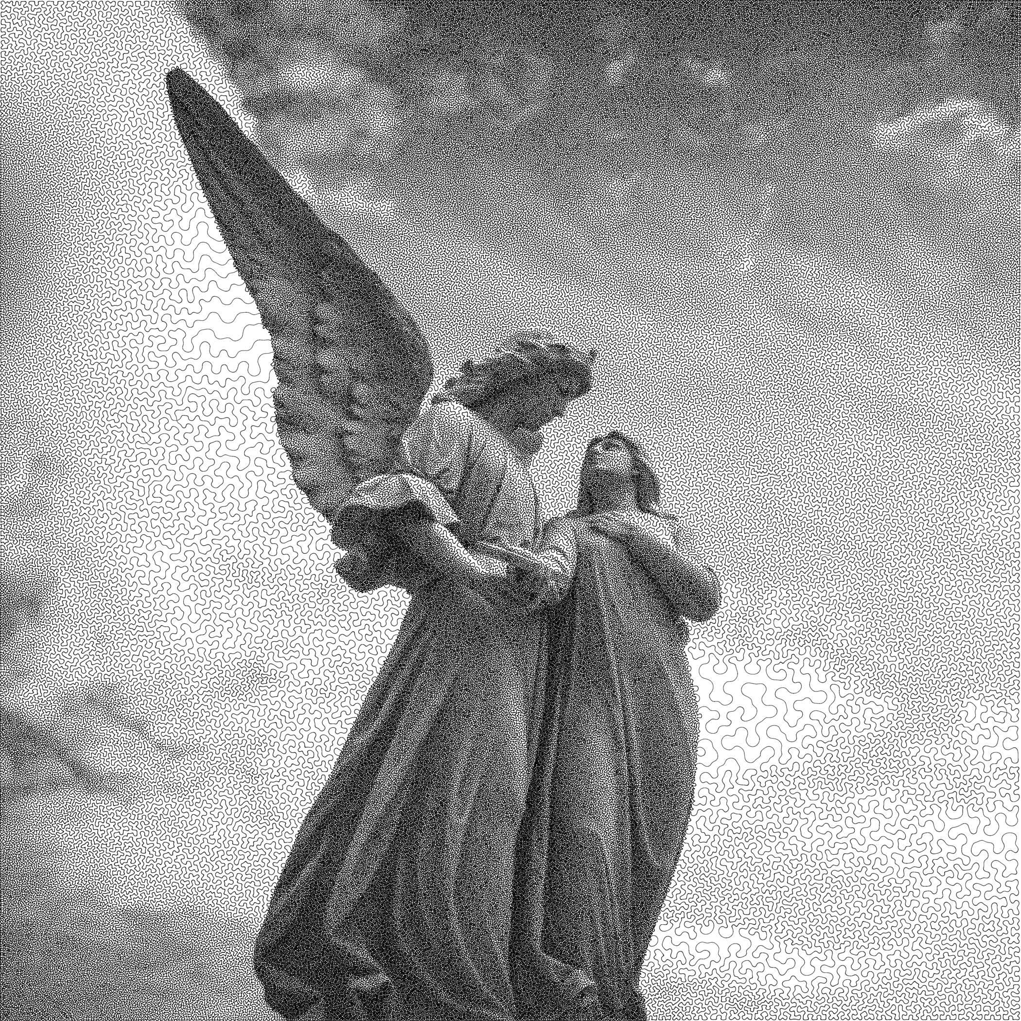
(b) Curve length $l$

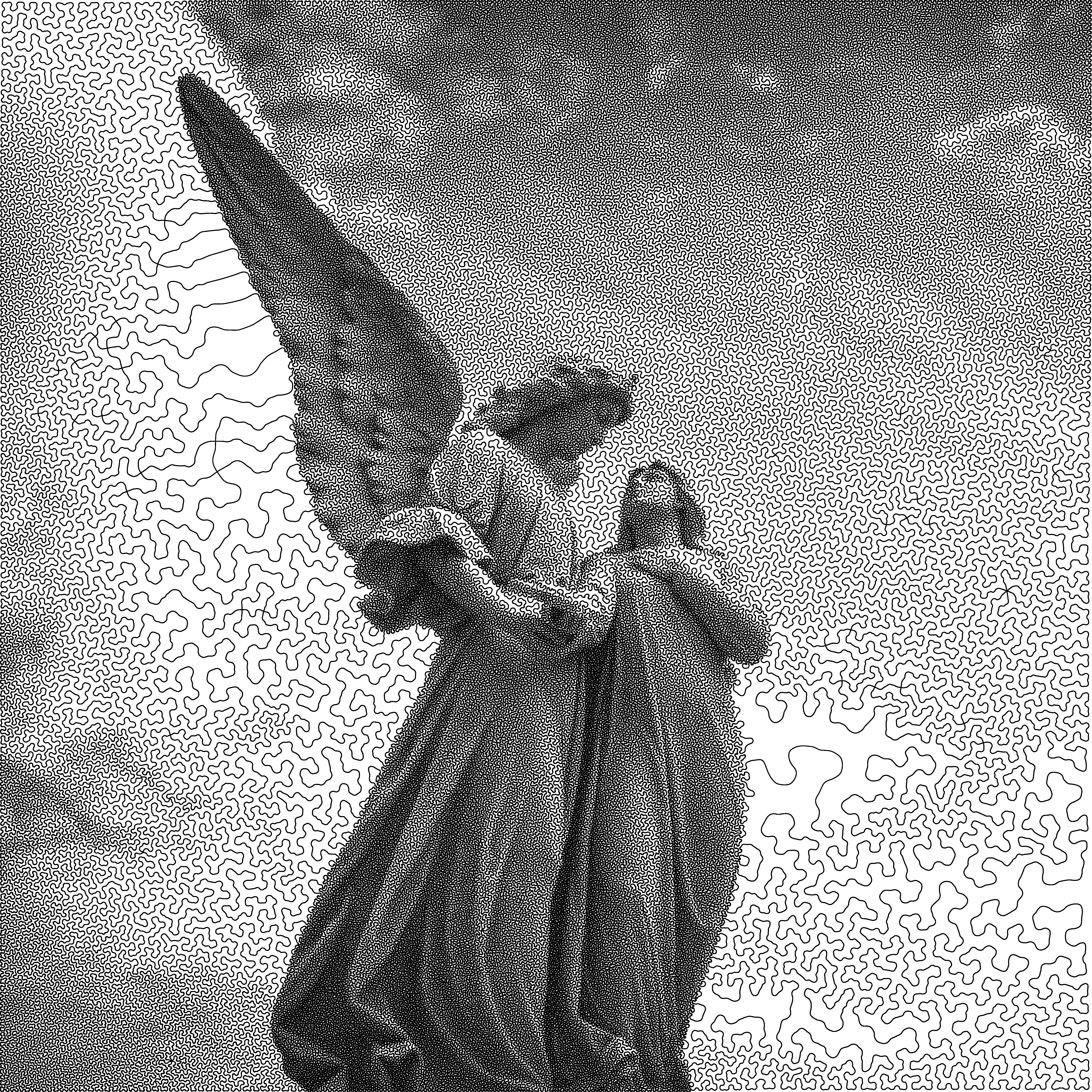
(c) Curve length $\frac{l}{3}$

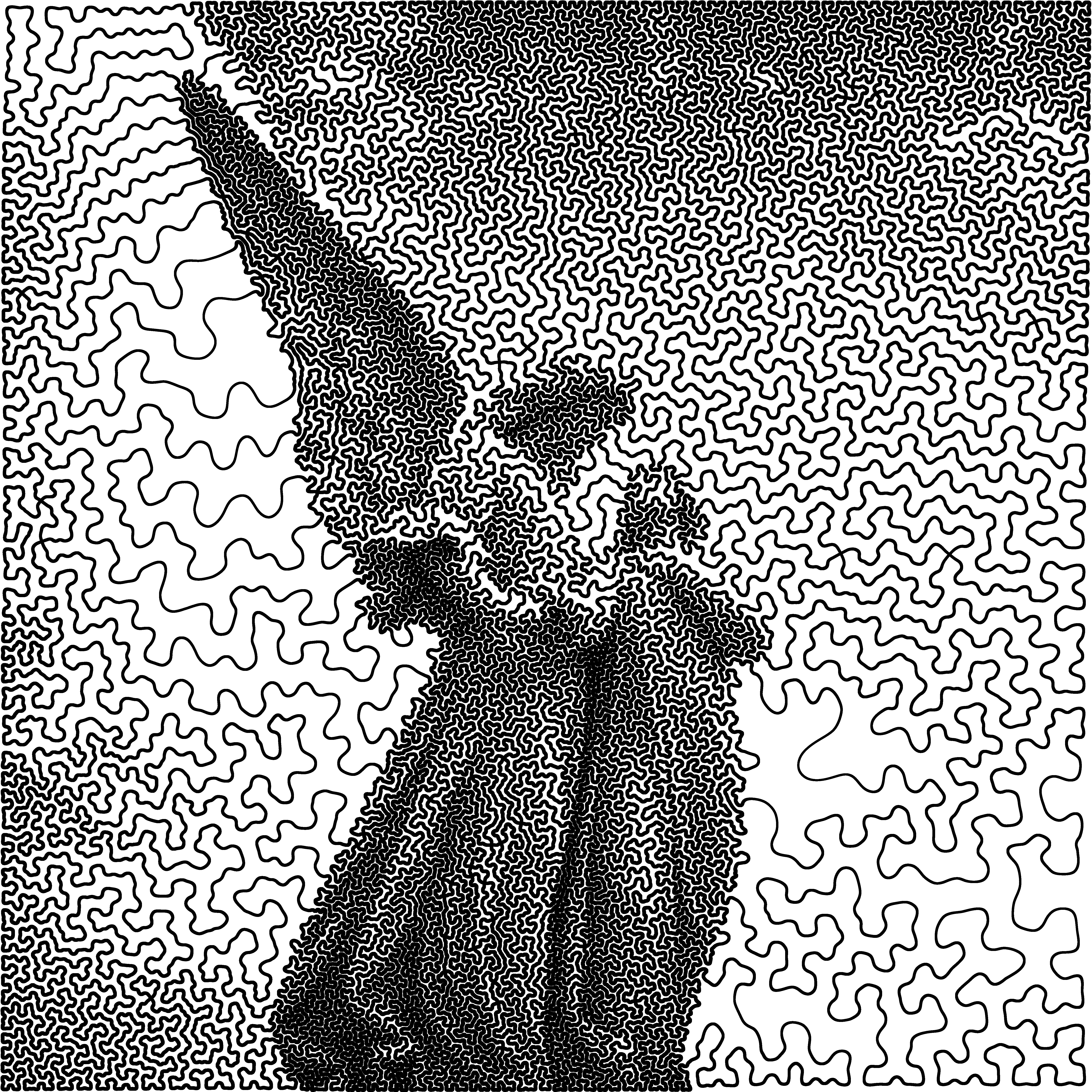
(d) Curve length $\frac{l}{12}$

Figure 5: Examples of Curvling (stippling + curve projection, 256k, $\approx$ 10’),

7.1.2 Color images

There are different ways to render color images with the proposed idea. We refer for instance to [60, 9] for two different examples. In this section, we propose a simple alternative idea to give a color to the dots or curves. Given a target vectorial density $\rho=(\rho_{R},\rho_{G},\rho_{B}):\Omega\to[0,1]^{3}$, the algorithm we propose simply reads as follows:

1. We first construct a gray level image defined by:

   $$\bar{\rho}=(\rho_{R}+\rho_{G}+\rho_{B})/3.$$ (44)

2. Then, we project the density $\bar{\rho}$ onto the set of constraints $\mathcal{M}$ with Algorithm 1. This yields a sequence of points $\mathbf{x}\in\Omega^{n}$.

3. Then, for each point $\mathbf{x}[i]$ of the discretized measure, we select a color as $\frac{\rho(\mathbf{x}[i])}{\bar{\rho}(\mathbf{x}[i]))}$.

We use only saturated colors, explaining the division in step 3). The parallel for gray-scale images, is that we represent stippling results with disks taking only the maximal intensity. Then, the mean in step 1) is used to attract the curve towards the regions of high luminance of the image. An example of result of the proposed algorithm is shown in Figure 6.

(a) Target color image

(b) Approximate color measure

Figure 6: Examples of color curvling, 512k, $\approx$ 24’),

7.1.3 Dynamic examples

The codes can also be used to approximate videos. The principle is simple: first we approximate the first sequence of the frame with our projection algorithm starting from an arbitrary initial guess. Then, the other frames are obtained with the projection algorithm, taking as an initial guess, the result of the previous iteration. This ensures some continuity of the dots or curves between consecutive frames. Some videos are given in the supplementary material.

7.2 Path planning

In this section, we provide two applications of the proposed algorithm to path planning problems.

7.2.1 Videodrone

Drone surveillance is an application with increasing interest from cities, companies or even private individuals. In this paragraph, we show that the proposed algorithms can be used to plan the drone trajectories for surveillance applications. We use the criminal data provided by [13] to create a density map of crime in Philadelphia, see Fig. 7a. We give different weights to different types of crimes. By minimizing (1), we can design an optimal path, in the sense that it satisfies the kinematic constraints of the drone and passes close to dangerous spots more often than in the remaining locations. In this example, we impose a bounded speed, a maximal yaw angular velocity and also to pass at a given location at a given time to recharge the drone to satisfy autonomy constraints.

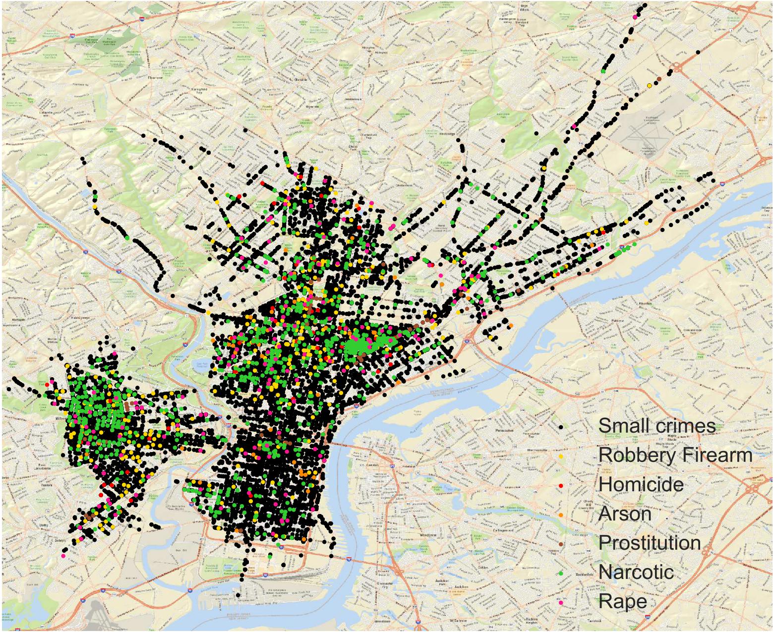
(a) The crime density $\mu$

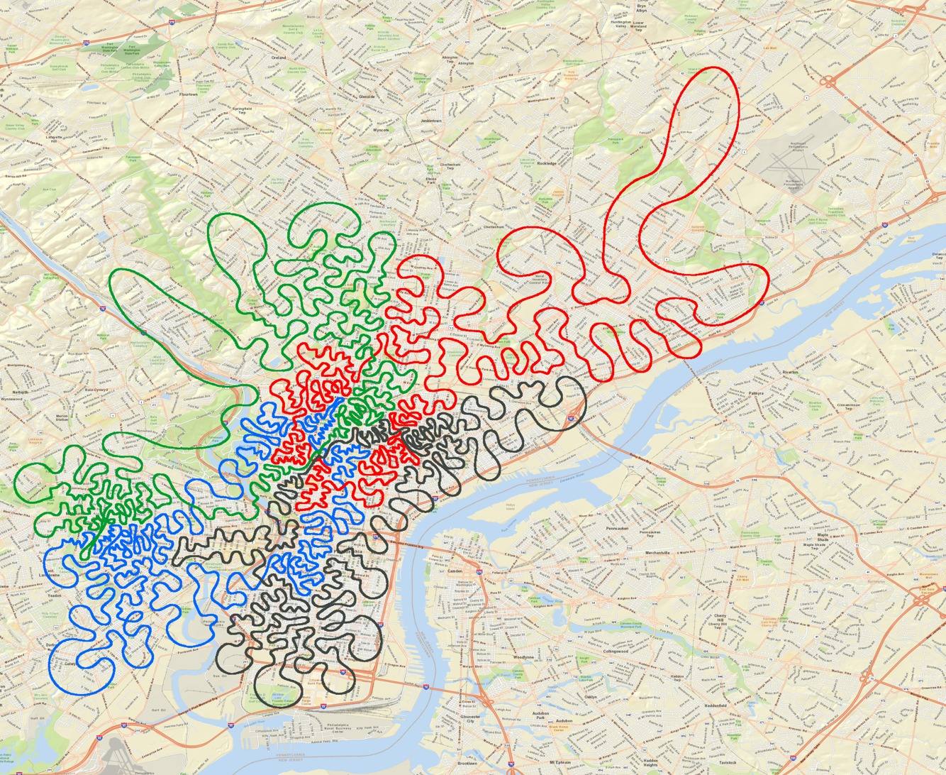
(b) Path adopted by the drone

Figure 7: The data superimposed on a map of Philadelphia. A possible drone trajectory made. In this example, the drone passes 4 times to its recharging location, explaining the different colors of the trajectory. In this example, the trajectory was discretized with 8k points and optimized in 30”.

7.2.2 Laser engraving

In Fig. 8, we gave a trajectory to a laser engraving machine in order to reproduce a landscape with a continuous line. We suspect that the same techniques could be used to optimize the nozzle and the flow of matter trajectory of 3D printers.

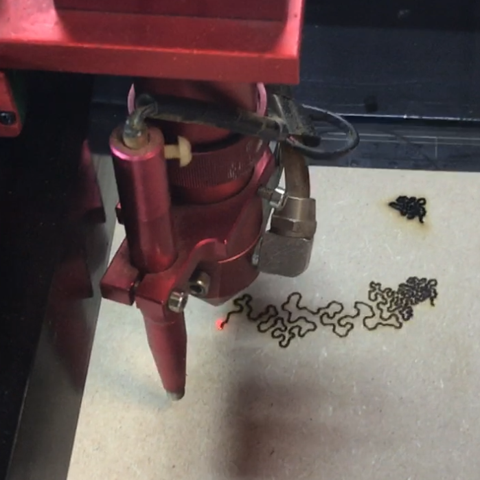
(a) Laser engraving machine

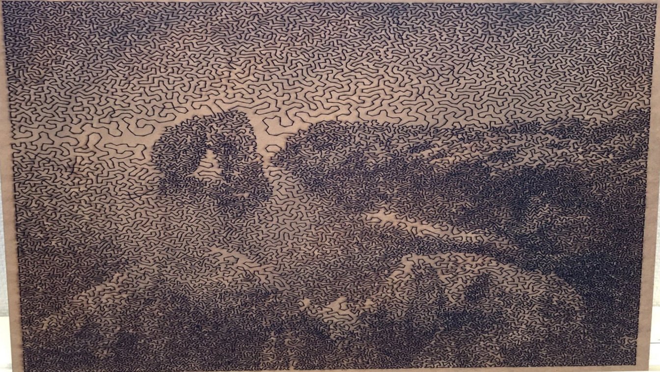
(b) The resulting wood engraved trajectory

Figure 8: Example of wood engraving. Left: a laser burning the wood by following an input trajectory. Right: the final result.

7.2.3 Sampling in MRI

Following [7], we propose to generate compressive sampling schemes in MRI (Magnetic Resonance Imaging), using the proposed algorithm.

In MRI, images are probed indirectly through their Fourier transform. Fourier transform values are sampled along curves with bounded speed and bounded acceleration, which exactly corresponds to the set of constraints defined in (31). The latest compressed sensing theories suggest that a good way of subsampling the Fourier domain, consists in drawing points independently at random according to a certain distribution $\mu$, that depends on the image sparsity structure in the wavelet domain [7, 1]. Unfortunately, this strategy is impractical in MRI due to physical constraints. To simulate such a sampling scheme, we therefore propose to project $\mu$ onto the set of admissible trajectories.

Let $u:[0,1]^{2}\to\mathbb{R}$ denote a magnetic resonance image. The sampling process yields a set of Fourier transform values $\mathbf{y}[i]=\hat{u}(\mathbf{x}[i])$. Given this set of values, the image is then reconstructed by solving a nonlinear convex programming problem:

$$\min_{v,v|_{\mathbf{x}}=\mathbf{y}}\frac{1}{2}\|\hat{v}(\mathbf{x})-\mathbf{y}\|_{2}^{2}+\lambda\|\Psi u\|_{1},$$ (45)

where $\Psi$ is a linear sparsifying transform, such as a redundant wavelet transform.

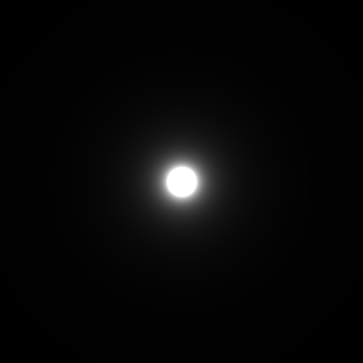
(a) Target density $\mu$

(b) Sampling scheme

(c) True image

(d) Reconstructed image

Figure 9: Example of sampling scheme generation and image reconstruction in MRI. The target density $\mu$ is shown in 9a. The sampling scheme generated by our algorithm is shown in 9b. The background shows the Fourier transform of $u$ in log-scale. It contains one fourth of the total number of Fourier transform values. The true image and the reconstructed one are shown in Fig. 9c and 9d.

Appendix A Theoretical convergence of Algorithm 1

The following result is a direct application of standard convergence results, see e.g. [44].

Theorem 3.

Suppose that $X\subset\mathbb{R}^{n}$ is closed and convex, that $\Sigma_{k}=\Sigma$ is a constant positive definite matrix. In addition, suppose that $F$ is a $C^{1}$ function with Lipschitz continuous gradient:

$$\forall(\mathbf{x}_{1},\mathbf{x}_{2}),\|\nabla F(\mathbf{x}_{1})-\nabla F(\mathbf{x}_{2})\|_{\Sigma^{-1}}\leq L\|\mathbf{x}_{1}-\mathbf{x}_{2}\|_{\Sigma}.$$ (46)

Finally suppose that either $X$ is compact or $F$ is coercive. Then Algorithm 1 converges to a critical point of $F$ for step-size $s_{k}=\frac{1}{L}$.

Applying Theorem 3 requires $\Sigma_{k}$ to be constant, hence the mass $\mathbf{w}$ to be prescribed. We make this assumption in this section.

Theorem 3 shows that it is critical to evaluate - if it exists - the Lipschitz constant of $\nabla_{\mathbf{x}}F$. By equation (23), we need to evaluate the variations of the Laguerre cells barycenter $\mathbf{b}$ with respect to $\mathbf{x}$. Unfortunately, following the Hessian computation in [16], the Lipschitz constant scales as $\min_{i\neq j}\|\mathbf{x}[i]-\mathbf{x}[j]\|^{-1}$ and cannot be proven to be uniform in $\mathbf{x}$. Hence, we can only hope for a local result describing the Lipschitz constant.

Hence, if the hypothesis of existence of the Hessian of $F$ are met (see [16]), an estimation of the Lipschitz constant of $F$ by its Hessian yields a theory of local convergence of $F$ in a vicinity $\mathcal{V}(\mathbf{x}^{*})$ of a local minimizer $\mathbf{x}^{*}$, for small enough steps $s_{k}$. Without these assumptions, local Lipschitz continuity of the gradient of $F$ cannot be enforced.

If in addition there is no $\Pi$-step, that is $X=\Omega^{n}$, the gradient of $F$ is $1$-Lipschitz around critical points (the so-called centroidal tessellation), see [18, Prop. 6.3]. Hence, convergence can be proven in a vicinity of $\mathbf{x}^{*}$ for step choice $s_{k}=1$ and the metric $\Sigma_{k}$. However, the size of the vicinity $\mathcal{V}(\mathbf{x}^{*})$ relies on the geometrical properties of the “optimal” Laguerre tessellation. The quality of such a local minimum could be very far from the global minimizer, nevertheless numerical experiments tend to indicate that is it not the case. For the same problem, hundreds of random initializations converge to a set of stationary points with a nice visual property.

References

- [1] B. Adcock, A. C. Hansen, C. Poon, and B. Roman. Breaking the coherence barrier: A new theory for compressed sensing. In Forum of Mathematics, Sigma, volume 5. Cambridge University Press, 2017.
- [2] E. Akleman, Q. Xing, P. Garigipati, G. Taubin, J. Chen, and S. Hu. Hamiltonian cycle art: Surface covering wire sculptures and duotone surfaces. Computers & Graphics, 37(5):316–332, 2013.
- [3] F. Aurenhammer. Power diagrams: properties, algorithms and applications. SIAM Journal on Computing, 16(1):78–96, 1987.
- [4] F. Aurenhammer. Voronoi diagrams—a survey of a fundamental geometric data structure. ACM Computing Surveys (CSUR), 23(3):345–405, 1991.
- [5] F. Aurenhammer, F. Hoffmann, and B. Aronov. Minkowski-type theorems and least-squares clustering. Algorithmica, 20(1):61–76, 1998.
- [6] M. Balzer, T. Schlömer, and O. Deussen. Capacity-constrained point distributions: a variant of Lloyd’s method, volume 28. ACM, 2009.
- [7] C. Boyer, N. Chauffert, P. Ciuciu, J. Kahn, and P. Weiss. On the generation of sampling schemes for magnetic resonance imaging. SIAM Journal on Imaging Sciences, 9(4):2039–2072, 2016.
- [8] C. Boyer, P. Weiss, and J. Bigot. An algorithm for variable density sampling with block-constrained acquisition. SIAM Journal on Imaging Sciences, 7(2):1080–1107, 2014.
- [9] N. Chauffert, P. Ciuciu, J. Kahn, and P. Weiss. Comment représenter une image avec un spaghetti? In GRETSI, 2015.
- [10] N. Chauffert, P. Ciuciu, J. Kahn, and P. Weiss. A projection method on measures sets. Constructive Approximation, 45(1):83–111, 2017.
- [11] N. Chauffert, P. Weiss, J. Kahn, and P. Ciuciu. Gradient waveform design for variable density sampling in Magnetic Resonance Imaging. arXiv preprint arXiv:1412.4621, 2014.
- [12] Z. Chen, Z. Shen, J. Guo, J. Cao, and X. Zeng. Line drawing for 3D printing. Computers & Graphics, 2017.
- [13] City of Philadelphia. Open data in the philadelphia region. https://www.opendataphilly.org/dataset/crime-incidents, 2017.
- [14] P. L. Combettes and J.-C. Pesquet. Proximal splitting methods in signal processing. In Fixed-point algorithms for inverse problems in science and engineering, pages 185–212. Springer, 2011.
- [15] F. De Goes, K. Breeden, V. Ostromoukhov, and M. Desbrun. Blue noise through optimal transport. ACM Transactions on Graphics (TOG), 31(6):171, 2012.
- [16] F. de Gournay, J. Kahn, and L. Lebrat. Differentiation and regularity of semi-discrete optimal transport with respect to the parameters of the discrete measure. arXiv preprint arXiv:1803.00827, 2018.
- [17] J. B. Du. Interactive Media Arts. https://jackbdu.wordpress.com/category/ima-capstone/, 2017.
- [18] Q. Du, V. Faber, and M. Gunzburger. Centroidal Voronoi tessellations: Applications and algorithms. SIAM review, 41(4):637–676, 1999.
- [19] L. C. Evans, J. Spruck, et al. Motion of level sets by mean curvature I. J. Diff. Geom, 33(3):635–681, 1991.
- [20] R. W. Floyd. An adaptive algorithm for spatial gray-scale. In Proc. Soc. Inf. Disp., volume 17, pages 75–77, 1976.
- [21] M. Fornasier, J. Haškovec, and G. Steidl. Consistency of variational continuous-domain quantization via kinetic theory. Applicable Analysis, 92(6):1283–1298, 2013.
- [22] W. Gangbo and R. J. McCann. The geometry of optimal transportation. Acta Mathematica, 177(2):113–161, 1996.
- [23] M. T. Gastner and M. Newman. Optimal design of spatial distribution networks. Physical Review E, 74(1):016117, 2006.
- [24] P. Giselsson and S. Boyd. Linear convergence and metric selection for douglas-rachford splitting and ADMM. IEEE Transactions on Automatic Control, 62(2):532–544, 2017.
- [25] R. Glowinski. On alternating direction methods of multipliers: a historical perspective. In Modeling, simulation and optimization for science and technology, pages 59–82. Springer, 2014.
- [26] G. N. Grapiglia and Y. Nesterov. Regularized Newton Methods for Minimizing Functions with Hölder Continuous Hessians. SIAM Journal on Optimization, 27(1):478–506, 2017.
- [27] L. Greengard and V. Rokhlin. A fast algorithm for particle simulations. Journal of computational physics, 73(2):325–348, 1987.
- [28] A. Hertzmann. A survey of stroke-based rendering. IEEE Computer Graphics and Applications, 23(4):70–81, July 2003.
- [29] S. Hiller, H. Hellwig, and O. Deussen. Beyond stippling—methods for distributing objects on the plane. In Computer Graphics Forum, volume 22, pages 515–522. Wiley Online Library, 2003.
- [30] F. Jarre and P. L. Toint. Simple examples for the failure of Newton’s method with line search for strictly convex minimization. Mathematical Programming, 158(1-2):23–34, 2016.
- [31] L. V. Kantorovich. On the translocation of masses. In Dokl. Akad. Nauk. USSR (NS), volume 37, pages 199–201, 1942.
- [32] C. S. Kaplan, R. Bosch, et al. TSP art. In Renaissance Banff: Mathematics, music, art, culture, pages 301–308. Bridges Conference, 2005.
- [33] S. Y. Kim, R. Maciejewski, T. Isenberg, W. M. Andrews, W. Chen, M. C. Sousa, and D. S. Ebert. Stippling by example. In Proceedings of the 7th International Symposium on Non-Photorealistic Animation and Rendering, pages 41–50. ACM, 2009.
- [34] J. Kitagawa, Q. Mérigot, and B. Thibert. A Newton algorithm for semi-discrete optimal transport. arXiv preprint arXiv:1603.05579, 2016.
- [35] B. Lévy. A numerical algorithm for L2 semi-discrete optimal transport in 3D. ESAIM: Mathematical Modelling and Numerical Analysis, 49(6):1693–1715, 2015.
- [36] B. Lévy and E. L. Schwindt. Notions of optimal transport theory and how to implement them on a computer. Computers & Graphics, 72:135–148, 2018.
- [37] G. Li and T. K. Pong. Global convergence of splitting methods for nonconvex composite optimization. SIAM Journal on Optimization, 25(4):2434–2460, 2015.
- [38] S. Lloyd. Least squares quantization in PCM. IEEE transactions on information theory, 28(2):129–137, 1982.
- [39] M. McAsey and L. Mou. Optimal locations and the mass transport problem. Contemporary Mathematics, 226:131–148, 1999.
- [40] Q. Mérigot. A multiscale approach to optimal transport. Computer Graphics Forum, 30(5):1583–1592, 2011.
- [41] Q. Mérigot, J. Meyron, and B. Thibert. An algorithm for optimal transport between a simplex soup and a point cloud. SIAM Journal on Imaging Sciences, 11(2):1363–1389, 2018.
- [42] L. Moisan. Affine plane curve evolution: A fully consistent scheme. IEEE Transactions on Image Processing, 7(3):411–420, 1998.
- [43] G. Monge. Mémoire sur la théorie des déblais et des remblais. De l’Imprimerie Royale, 1781.
- [44] Y. Nesterov. Gradient methods for minimizing composite functions. Mathematical Programming, 140(1):125–161, 2013.
- [45] Y. Nesterov. Introductory lectures on convex optimization: A basic course, volume 87. Springer Science & Business Media, 2013.
- [46] R. Nishihara, L. Lessard, B. Recht, A. Packard, and M. I. Jordan. A General Analysis of the Convergence of ADMM. In ICML, pages 343–352, 2015.
- [47] G. Pages and B. Wilbertz. Optimal Delaunay and Voronoi quantization schemes for pricing American style options. In Numerical methods in Finance, pages 171–213. Springer, 2012.
- [48] R. Peyre. Comparison between distance and -norm, and localisation of wasserstein distance. 2016.
- [49] R. A. Polyak. Regularized newton method for unconstrained convex optimization. Mathematical programming, 120(1):125–145, 2009.
- [50] D. Potts and G. Steidl. Fast summation at nonequispaced knots by NFFT. SIAM Journal on Scientific Computing, 24(6):2013–2037, 2003.
- [51] S. Schlechtweg, T. Germer, and T. Strothotte. RenderBots Multi-Agent Systems for Direct Image Generation. In Computer Graphics Forum, volume 24, pages 137–148. Wiley Online Library, 2005.
- [52] C. Schmaltz, P. Gwosdek, A. Bruhn, and J. Weickert. Electrostatic halftoning. In Computer Graphics Forum, volume 29, pages 2313–2327. Wiley Online Library, 2010.
- [53] J. Solomon, F. De Goes, G. Peyré, M. Cuturi, A. Butscher, A. Nguyen, T. Du, and L. Guibas. Convolutional Wasserstein distances: Efficient optimal transportation on geometric domains. ACM Transactions on Graphics (TOG), 34(4):66, 2015.
- [54] A. Tagliasacchi, I. Alhashim, M. Olson, and H. Zhang. Mean curvature skeletons. In Computer Graphics Forum, volume 31, pages 1735–1744. Wiley Online Library, 2012.
- [55] T. Teuber, G. Steidl, P. Gwosdek, C. Schmaltz, and J. Weickert. Dithering by differences of convex functions. SIAM Journal on Imaging Sciences, 4(1):79–108, 2011.
- [56] The CGAL Project. CGAL User and Reference Manual. CGAL Editorial Board, 4.9 edition, 2016.
- [57] R. Ulichney. Digital halftoning. MIT press, 1987.
- [58] C. Villani. Topics in optimal transportation. Number 58. American Mathematical Soc., 2003.
- [59] C. Villani. Optimal transport: old and new, volume 338. Springer Science & Business Media, 2008.
- [60] L.-Y. Wei. Multi-class blue noise sampling. ACM Transactions on Graphics (TOG), 29(4):79, 2010.
- [61] S. J. Wright and J. Nocedal. Numerical optimization. Springer Science, 35(67-68):7, 1999.
- [62] S.-Q. Xin, B. Lévy, Z. Chen, L. Chu, Y. Yu, C. Tu, and W. Wang. Centroidal power diagrams with capacity constraints: computation, applications, and extension. ACM Transactions on Graphics (TOG), 35(6):244, 2016.
- [63] A. Yezzi. Modified curvature motion for image smoothing and enhancement. IEEE Transactions on Image Processing, 7(3):345–352, 1998.