Unstable Periodically Forced Navier-Stokes Solutions—Towards Nonlinear First-Principle Reduced-Order Modeling of Actuator Performance

Abstract

We advance the computation of physical modal expansions for unsteady incompressible flows. Point of departure is a linearization of the Navier-Stokes equations around its fixed point in a frequency domain formulation. While the most amplified stability eigenmode is readily identified by a power method, the technical challenge is the computation of more damped higher-order eigenmodes. This challenge is addressed by a novel method to compute unstable periodically forced solutions of the linearized Navier-Stokes solution. This method utilizes two key enablers. First, the linear dynamics is transformed by a complex shift of the eigenvalues amplifying the flow response at the given frequency of interest. Second, the growth rate is obtained from an iteration procedure. The method is demonstrated for several wake flows around a circular cylinder, a fluidic pinball, i.e. the wake behind a cluster of cylinders, a wall-mounted cylinder, a sphere and a delta wing. The example of flow control with periodic wake actuation and forced physical modes paves the way for applications of physical modal expansions. These results encourage Galerkin models of three-dimensional flows utilizing Navier-Stokes based modes.

1 Introduction

Modeling instabilities and subsequent soft or hard bifurcations is at the heart of understanding laminar, transitional and turbulent flow dynamics. Many prominent coherent structures arise from instabilities. Well studied examples are the von Kármán vortex street behind cylinders, the Kelvin-Helmholtz vortices of mixing layers, the Tollmien-Schlichting waves in laminar boundary layers, the Taylor-Couette vortices between two centered rotating cylinders, the Görtler vortices in a boundary layer of an inward curved surface, and the Raleigh-Bénard cells in a horizontal plane fluid layer heated from below, just to name a few.

Many of these coherent structures also characterize the turbulent flow at Reynolds numbers which are orders of magnitudes beyond the bifurcation values. These observations have fueled a hypothesis in the 1940’s that turbulence may be the infinite succession of Hopf bifurcations Landau1944 ; Hopf1948 . In the 1980’s other transition scenarios have been added leading to strange attractors. Prominent examples are the Feigenbaum Feigenbaum1978jsp , Ruelle-Takens Ruelle1971cmp , Ruelle-Takens-Newhouse Newhouse1978cmp and Manneville-Pomeau scenario Pomeaou1980cmp . The list of transition scenarios could easily be extended.

The engineering relevance of these pioneering works to turbulence is rather limited, because the applicability is restricted to few configurations and a narrow Reynolds number regimes. Yet, these studies have provided important qualitative insights into the flow dynamics, like the notion of divergent trajectories, strange attractors, manifolds, domains of attraction, edge states, just to a name a few. In addition, the instabilities of laminar flows, like boundary-layer transition, is quantitatively characterized by stability analysis and has important engineering applications.

The interest in modal analysis of flows is twofold. Modal analysis is a tool for investigation of flow phenomena. On the other hand it is of vital interest for flow control. Physical modes were characterized above—there are modes which we are able to trigger in the flow field with an actuation. If the actuation is random and small the flow responds with the leading eigenmodes. However, the flow may respond to strong actuation with non-leading and sometimes local eigenmodes. Control strategies often take advantage of non-leading modes to control the dominating ones via frequency crosstalk. In this contribution, such a technique will be encapsulated in a nonlinear first-principle reduced-order model using tools of stability analysis. The use of physical modes—the leading and the non-leading ones is even more important for closed-loop, model-based control. To build a controller, the high- or infinite-dimensional system is projected onto a set of modes — of empirical, physical or mathematical type — to obtain a least-dimensional representation. The use of physical modes in this situation may be more effective to represent flow response than employing a large number of mathematical or empirical modes.

Another enabling aspect of stability analyses is that the resulting eigenmodes may be suited for Galerkin models describing flow dynamics beyond the assumptions of bifurcation theory. One example is the Galerkin model over a separated boundary layer Akervik2007jfm or vortex shedding behind a wake Noack2003jfm . For simple configurations, stability eigenmodes have be shown to form a basis for arbitrary flows Grosch1978jfm ; Salwen1981jfm or distill at least the dominant coherent structures. Alternative data-driven to first-principle-based expansions are discussed in Taira2018arXiv . The dominant one-global stability eigenmodes are easy to compute while Bi- and Tri–global modes—following the terminology of Theofilis theofilis2003advances ; Theofilis2011arfm (meaning fully two–dimensional or fully three–dimensional) stability analysis provide a significant challenge.

This study is devoted to advancing the computation on several stability eigenmodes for complex three-dimensional flows. Our investigation of linearized Navier-Stokes equations assesses either global modes of the flow or responses to a particular perturbation. Contrary to receptivity studies, we analyze Navier-Stokes perturbation equation in frequency domain and apply a complex shift to narrow down the investigated frequency range. The analysis employs elements of our earlier methods of global (fully two–dimensional or fully three–dimensional) flow stability investigations, elements of our shift- inverse ZAMM89 , subspace methodology MORZYNSKI1999 and three-dimensional numerical solutions Morzynski2008gdansk . It is following the spirit and directions of gomez2015use ; LIU2016316 ; semeraro_bagheri_brandt_henningson_2011 ; garnaud_lesshafft_schmid_huerre_2013 ; åkervik_hœpffner_ehrenstein_henningson_2007 ; chomaz2005global .

The manuscript is outlined as follows: Section 2 details the proposed methodology starting from frequency domain formulation of the linearized Navier-Stokes equations. Sections 3 and 4 describe investigations of two- and three-dimensional wake flows, respectively. Section 5 shows the example of reduced-order modeling of periodic wake actuation with the technique of forced physical modes, developed in previous sections. In the conclusions (Sec. 6), we summarize the study and outline perspectives for future work.

2 Frequency Domain Formulation and Solution

2.1 Navier-Stokes Equations in Frequency Domain

We focus on incompressible flows around obstacles in a steady domain $\Omega$. The Newtonian fluid is characterized by the constant density $\rho$ and kinematic viscosity $\nu$. The flow is described in a Cartesian coordinate system ${\bf x}=(x,y,z)=(x_{1},x_{2},x_{3})$ with corresponding velocity vector ${\bf V}=(V_{1},V_{2},V_{3})$ and pressure $P$. The time is represented by $t$ and the volume force by ${\bf F}=(F_{1},F_{2},F_{3})$. In the sequel, all quantities are assumed to nondimensionalized with density $\rho$, the characteristic velocity $U$ and characteristic length $L$. Thus, the flow solution is parameterized by the Reynolds number

$$Re=\frac{UL}{\nu}.$$ (1)

The evolution is described by the Navier-Stokes equations

$$\dot{V}_{i}+V_{i,j}V_{j}+P_{,i}-\frac{1}{Re}V_{i,jj}=F_{i}$$ (2)

and equation of continuity

$${V}_{i,i}=0.$$ (3)

Here the dot denotes temporal differentiation, the superscript ‘$,i$’ denotes partial differentiation with respect to $x_{i}$ and ‘$,ii$’ double partial differentiation with respect to $x_{i}$.

The steady solution of (2) is indicated by a bar, i.e. $\bar{V}_{i}$ and $\bar{P}$ denote the velocity component and pressure under the steady force $\bar{F}$. We decompose the flow variables in a steady component and disturbance indicated by an acute symbol:

$$V_{i} = \bar{V_{i}}+\acute{V_{i}}$$ (4a)

$$P = \bar{P}+\acute{P}$$ (4b)

$$F = \bar{F}+\acute{F}.$$ (4c)

The evolution equation of the disturbance is derived from substituting (4) in (2) and subtracting the steady Navier-Stokes equations. The corresponding Navier-Stokes equation and equation of continuity read

$$\dot{\acute{V}_{i}}+\acute{V}_{j}\bar{V}_{i,j}+\bar{V}_{j}\acute{V}_{i,j}+\acute{V}_{j}\acute{V}_{i,j}+\acute{P}_{,i}-\frac{1}{Re}\acute{V}_{i,jj}=\acute{F}_{i}$$ (5)

and

$$\acute{V}_{i,i}=0.$$ (6)

Equation (5) has linear terms in velocity, pressure and force and one quadratic term in the velocity. Close to the steady solution, the quadratic term $\acute{V}_{j}\acute{V}_{i,j}$ can be ignored, yielding the linearized Navier-Stokes equations.

In the next step, the disturbance is subjected to the separation ansatz in time and space dependence:

$$\acute{V}_{i}(x,y,z,t) = \tilde{V}_{i}(x,y,z)\,e^{\lambda t}+c.c.$$ (7)

$$\acute{P}(x,y,z,t) = \tilde{P}(x,y,z)\,e^{\lambda t}+c.c.$$

$$\acute{F}_{i}(x,y,z,t) = \tilde{F}_{i}(x,y,z)\,e^{\lambda t}+c.c.$$

where $e^{\lambda t}$ represents the temporal dynamics with complex eigenvalue $\lambda$ and the tilde marks the spatial amplitude of the mode. Now, the linearized evolution equations in the frequency domain read:

$$\lambda\tilde{V}_{i}+\tilde{V}_{j}\bar{V}_{i,j}+\bar{V}_{j}\tilde{V}_{i,j}+\tilde{P}_{,i}-\frac{1}{Re}\tilde{V}_{i,jj}=\tilde{F}_{i}$$

$$\tilde{V}_{i,i}=0.$$ (8)

The homogeneous form of equation (8) with vanishing force constitutes the generalized complex, nonhermitian eigenvalue problem. We use the penalty formulation of the Navier-Stokes equations for the examples presented here, i.e. for the steady base solution, eigensolutions, and unsteady computations. The penalty method eliminates the pressure from governing equations and enforces near incompressibility via:

$$\frac{1}{\epsilon}P=V_{j,j}$$ (9)

The penalty parameter $\epsilon$ is usually chosen to be a large number, related to computer word length. In the calculations presented in the following sections we assume $\epsilon=10^{5}$ and keep it constant in the iteration process. The Ladyzenskaja-Babuška-Brezzi (LBB) condition stating the allowable interpolating functions for velocity and pressure is, in the penalty formulation, equivalent to using a reduced integration of the penalty term. It should be mentioned that in other studies, including flow computations and eigenanalysis, we have used also the velocity-pressure Finite Element Method (FEM) formulation of the Navier-Stokes equations, obtaining almost identical results.

In compact form the equation (8) can be written as

$$\bf{Aq}+\lambda\bf{Bq}=F,$$ (10)

where $\bf{q}$ represents the flow variables $\tilde{V}$ and $\tilde{P}$, and $\bf{F}$ comprises $\tilde{F}_{i}$. From the considered solutions of equations (8) to (10) we exclude trivial ones. For all practical purposes, $\bf{q}$ and $\bf{F}$ denote the flow and force discretization on a grid, $\bf{A}$ represents the matrix associated with the linear Navier-Stokes dynamics and $\bf{B}$ the mass matrix.

After a realistic discretization of equations (8), the number of degrees of freedom (DOF), i.e. the dimension of $\bf{q}$, is usually very large, at least of order of $O\left(10^{5}\right)$ for two-dimensional and $0\left(10^{6}\right)$ for the three-dimensional problem. The corresponding eigenvalue problem constitutes a numerical challenge. Many eigenvalues $\lambda$ form complex conjugate pairs which causes additional problems for solution algorithms.

Instead of direct solution of the homogeneous eigenvalue problem, we investigate the flow response in frequency domain. In contrary to commonly employed ”black box”approaches we shall take advantage of knowledge of governing equations.

It is practical to split the complex equation (8) into two real-valued equations which read:

$${\bf Aq}_{Re}+\lambda_{Re}{\bf Bq}_{Re}+\lambda_{Im}{\bf Bq}_{Im} = {\bf F}_{Re}$$

$${\bf Aq}_{Im}+\lambda_{Re}{\bf Bq}_{Im}-\lambda_{Im}{\bf Bq}_{Re} = {\bf F}_{Im}.$$ (11)

The inverse of the complex system matrix of (11) plays the role of frequency response function relating the amplitudes and the phases of the system response with the forcing function.

2.2 Boundary Conditions

For the steady base solution, on the inflow, and on the upper, lower, front and back boundary, we set the Dirichlet boundary conditions:

$$V_{x}=1,\;V_{y}=0,\;V_{z}=0$$ (12)

where $x$ is the direction of the inflow. On the outflow of the domain we use the condition:

$$\int_{\Gamma}\Phi_{m}\sigma_{ij}n_{j}\,d\Gamma=0$$ (13)

where $\Phi$ is FEM weighting function, $\sigma_{ij}$ denotes the stress tensor and $n_{j}$ is the unit vector normal to the boundary $\Gamma$. It is the ”do nothing”, homogeneous Neumann, natural, non-reflecting boundary condition for the Finite Element Method, fully “transparent” to the flow. On the body, the no-slip boundary condition reads:

$$V_{x}=0,\;V_{y}=0,\;V_{z}=0.$$ (14)

For eigensolutions the homogeneous Dirichlet boundary conditions:

$$\tilde{V_{x}}=0,\;\tilde{V_{y}}=0,\;\tilde{V_{z}}=0$$ (15)

are set on the inflow, upper, lower, front and back boundaries. On the outflow the natural boundary conditions, analogous with those applied for steady flow, are introduced. The forced actuation in the frequency domain is equivalent to either Dirichlet boundary condition or inhomogeneous Neumann boundary condition. For example, the oscillatory motion of the cylinder, having diameter $D=1$, is introduced via setting

$$V_{x} = \quad 2A\,y_{C}$$ (16)

$$V_{y} = \,-2A\,x_{C}$$

where $A$ is the amplitude of the oscillation and $x_{C}$ and $y_{C}$ are the coordinates of a node on the cylinder surface. Inhomogeneous volume force can be set in the domain as the non-zero entrance to right hand side vector (RHS) of the Finite Element Method system. The indices and boundary conditions for the two-dimensional examples are limited only to the $x,y$ values.

2.3 Complex Shift

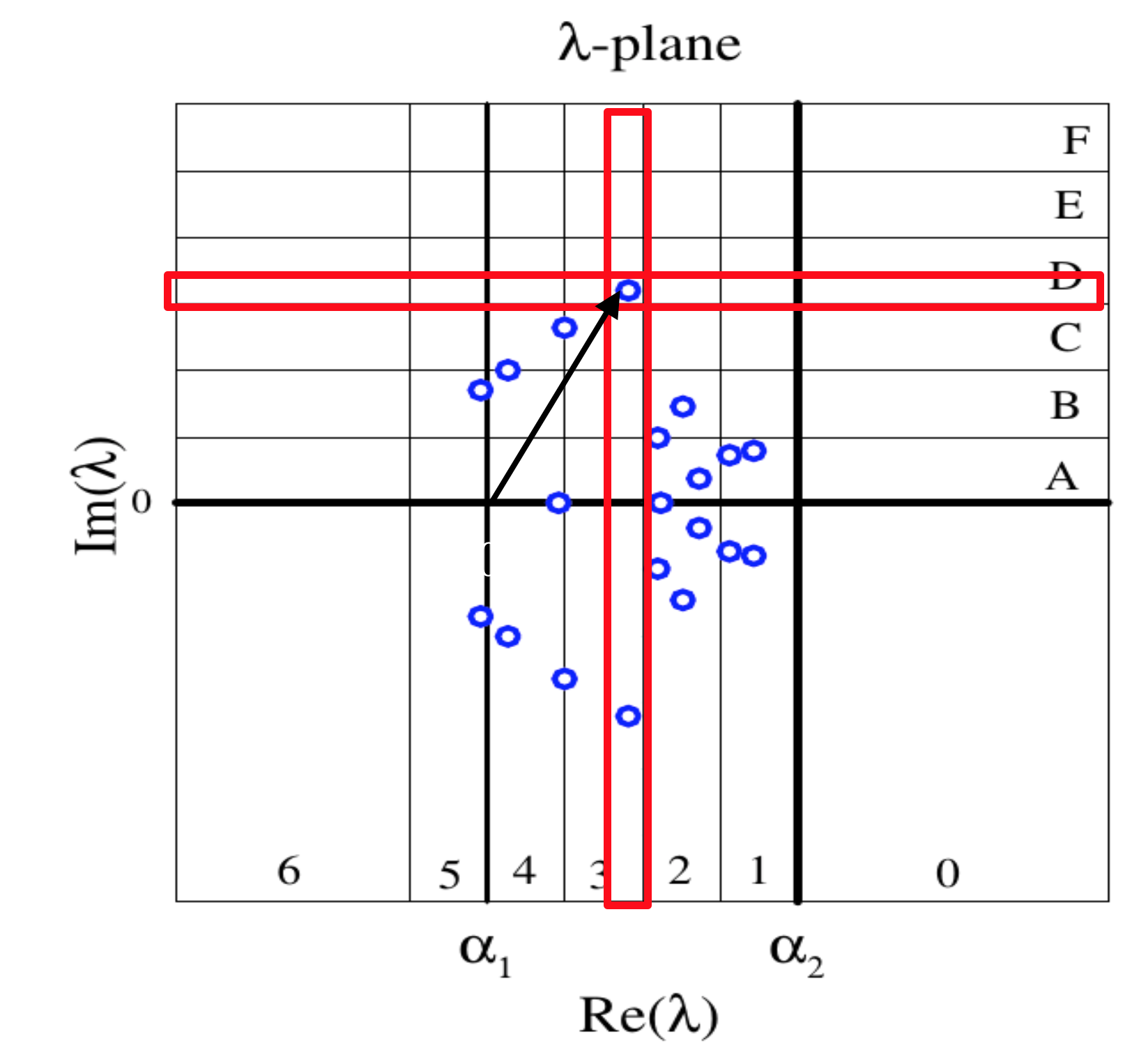
Figure 1: Complex shift for the eigenvalue spectrum of a circular cylinder at $Re=100$, adapted from MORZYNSKI1999 .

Let us assume that the approximate eigenvalue of interest $\mu$ is known and $\alpha$ is the difference to the accurate eigenvalue $\lambda$

$$\lambda=\mu+\alpha.$$ (17)

In this case, original eigenvalue problem (10) may be shifted

$$(\bf{A}+\alpha\bf{B}){\bf q}+\mu{\bf Bq}={\bf 0},$$ (18)

where we solve for the small error $\alpha$. Equation (17) allows us to reconstruct the eigenvalues for original system (10). The eigenvectors of original and shifted eigensystem are the same.

There are many advantages in the use of the shifted eigenvalue problem. The convergence of the approximated eigenvalue problem is much faster as it is for the original eigenvalue of the system. Second, the singularity or ill conditioning of the system matrix is avoided. Third and most importantly, we can choose the ”area of interest” in the eigenvalue spectrum.

This methodology is demonstrated in Fig. 1 and details were presented in MORZYNSKI1999 . The figure shows the eigenvalues for the circular cylinder flow at $Re=100$ in the complex plane. The horizontal, real axis refers to the growth rate of the eigenvalue while the vertical one corresponds to it’s frequency. With the complex shift, indicated in the figure by the arrow we can compute the eigensolution for arbitrary eigenvalues. This allows us to skip the most amplified eigenvalues, related to the von Kármán mode and focus on the other.

The technique of the complex shift can be also used if want to investigate the frequency transfer function for particular frequency and growth rate of the disturbance and this approximate is equal to $\alpha$.

$$(\bf{A}+\alpha\bf{B}){\bf q}+\mu{\bf Bq}={\bf F}.$$ (19)

The equation (19) represents the fluid flow in which all the oscillations except the ones close to $\alpha$ are eliminated or damped. The dominant mode (e.g. von Kármán mode for bluff bodies) which usually dominates and overrides all other modes is not triggered and we can find the (linear) response of shear layer or boundary layer to the actuation even if the corresponding eigenvalues are damped. This information can be relevant for the flow control as we can estimate the growth rate of the mode and the energy which should be delivered to the actuator for this mode to pop up. Actuating the additional modes can be essential in damping of the dominating, most energetic one. We can also optimize the approximate (linear) flow response as a function of actuator’s placement.

2.4 Structural Mechanics Analogy

Structural mechanics was one of the first technical fields which used modal analysis and reduced-order models (ROM). It employs methods and tools like static and dynamic condensation, modal coordinates reduction, component mode synthesis and the Ritz vector method. The latter is used to generate modes, approximate eigenvectors or define the transfer function of the system. All these problems are also important in fluid dynamics.

In the structural mechanics formulation, the homogeneous form of equation (11) is usually written as:

$${\bf Kx}-\omega_{c}^{2}\,{\bf Mx}={\bf 0},$$ (20)

where ${\omega_{c}^{2}}$ is equivalent to $-\lambda$, $\bf K$ denotes stiffness matrix and $\bf M$ is the mass matrix.

The solution method can be described as Ritz vector method. It has been used mainly in structural mechanics as the alternative or complement of modal approach qu2013model . In structural mechanics we apply static Ritz Vector Methods (RVM), often referred to as Wilson-Yuan-Dickens (WYD) approach wilson1982dynamic . WYD employs sequential solution of:

$$\hat{{\bf x}}_{1}={\bf K}^{-1}{\bf g}.$$ (21)

The inertia term, neglected in the first step is used to generate the new Ritz vectors:

$$\hat{{\bf x}}_{i}={\bf K}^{-1}{\bf M}\hat{{\bf\,x}}_{i-1}$$ (22)

with subsequent $\bf M$-normalization

$${\bf x}_{1}=\frac{\hat{{\bf x}}_{1}}{(\hat{{\bf x}}_{1}^{T}{\bf M}\,\hat{{\bf x}}_{1})^{\frac{1}{2}}}$$ (23)

and $\bf M$-orthonormalization

$${\bf\hat{{\bf x}}}_{i}=\tilde{{\bf x}}_{i}-\sum_{j=1}^{i-1}({\bf x}_{j}^{T}{\bf M}\tilde{{\bf x}}_{i}){\bf x}_{i-1}.$$ (24)

Lanczos procedure is also one of the possible choices. WYD looses its performance for larger amount of not orthogonal vectors. To alleviate this difficulty, the Load-Dependent-Ritz Vectors method (LDRV) is extended to so called quasi-static Ritz vector methods in which Ritz vector span the model space at desired prescribed frequencies to efficiently capture the dynamic response of the system at desired frequency qu2013model :

$$\hat{{\bf x}}_{1} = ({\bf K}-\omega_{c}^{2}\,{\bf M})^{-1}{\bf g}$$

$${\bf\tilde{{\bf x}}}_{i} = ({\bf K}-\omega_{c}^{2}\,{\bf M})^{-1}{\bf M}{\bf x}_{i-1}.$$ (25)

The first step obtained with this procedure represents the frequency response to the initial load. In the second step, the frequency response ${\bf x}_{2}$ of the system is enriched by additional inertial force of ${\bf M}{\bf x}_{i-1}$. After mass orthonormalization the new Ritz vector set spans a wider space of the dynamic response of the system qu2013model . The algorithms presented here can be used for finding the eigenvectors of the system.

There are similarities in the solution and transformation used in the presented procedure and iterative eigenvalue solvers. Similar procedures are applied for inverse iteration, subspace iteration and for the eigenvalue shift. For example, the subspace iteration forces the system with initial set of orthogonal vectors, which are becoming Ritz vectors during the iteration and eigenvectors at the end of the procedure. For generalized eigenvalue problem the $B$ matrix is used to transform the Ritz vectors to a new set, used in the next iteration. We use a single vector and do not compute the eigenvalue with the reduced model build on the space spanned by the Ritz vectors. The algorithm is very similar to Arnoldi iteration but uses shifted and inverted matrix and is applied to a generalized problem.

2.5 The Solution Algorithm

The above described methodology can be directly applied to create a modal basis and ROM of the fluid flow. Here, we adopt ideas of Quasi-Static Ritz Vector Method and Load-Dependent-Ritz Vectors method in the frequency domain. The methods were briefly introduced in Sect. 2.4. LDRV method was first introduced by Wilson Yuans and Dickens in wilson1982dynamic in structural dynamics. Ritz Vector Methods are generally used as the alternative to mode superposition. In this method the Ritz vectors are generated by loads, which translate in fluid dynamics to volume forces. Generation of load dependent Ritz vectors is far less computationally expensive than finding the eigenvectors and still spans the space adequate for accurate models.

In our approach the actuation of the flow is implemented with volume forces, acting either in discrete points or ones randomly distributed in the flow volume. Actuation can be also introduced as the Dirichlet boundary condition. It can be applied only in the first iteration, to trigger the flow response or can be held constant in all the iterations. Our system is complex and is characterized by frequency and growth rate. This distinguishes the approach from Static Ritz Vector method described above. We are forcing fluid motion not only at given frequency as in case described by equation (25) but also prescribe the real part of the eigenvalue damping or amplifying the fluid response.

In terms of eigenvalue solvers, we apply here the complex shift to the eigensystem of equations.

We disturb the flow with the volume force ${\bf Bq}_{Re}^{F}$ and ${\bf Bq}_{Im}^{F}$. Here, $\bf B$ can be considered the gain of a small random velocity ${\bf q}^{F}$ with support in the whole computational domain or a single point forcing. It should be noted that the introduced random disturbance has the frequency determined by $\lambda_{Im}$.

$${\bf Aq}_{Re}+\lambda_{Re}{\bf Bq}_{Re}+\lambda_{Im}{\bf Bq}_{Im} = -{\bf Bq}_{Re}^{F}$$

$${\bf Aq}_{Im}+\lambda_{Re}{\bf Bq}_{Im}-\lambda_{Im}{\bf Bq}_{Re} = -{\bf Bq}_{Im}^{F}.$$ (26)

The iteration with respect to $i$ is performed with

$${\bf Aq}^{(i)}+\lambda{\bf Bq}^{(i)}=-{\bf Bq}^{(i-1)}.$$ (27)

In the equation (27) we skip, for brevity of notation, the decomposition of complex equation to the two real number ones. The equation (27) implies the solution procedure. Once the initial volume force distribution is given it is placed in the right-hand side (RHS) of the equation (27). Also initial velocities, if given, can be transferred to the force value via the matrix $\bf B$ and placed in the RHS vector. The next step is the solution of the linear system of equations, giving the flow field response to the applied actuation. There is however another factor which has to be taken into account. For $\lambda$ we assumed the imaginary part $\lambda_{Im}$, being the angular frequency of the actuation. The real part, $\lambda_{Re}$ is unknown, being the parameter which has to be iteratively adjusted by the procedure. For this reason we must use an iterative approach, repeating the solution several times. To solve this problem we adopted the Newton-Raphson method implemented in our nonlinear Navier-Stokes solver:

$${\bf R}\left({\bf q}^{(i-1)}+\Delta{\bf q}\right) = {\bf R}({\bf q}^{(i-1)})+{\bf J}^{(i-1)}\Delta{\bf q}$$ (28)

$${\bf q}^{(i)} = {\bf q}^{(i-1)}-[{\bf J}^{(i-1)}]^{-1}{\bf R}({\bf q}^{(i-1)}),$$ (29)

where $\bf R$ represents the residuum of the equation (27), dependent on iterated $\lambda_{Re}$ and $\bf J$ is the Jacobian of the left-hand side of (27). Again, we replace the complex computations with the real arithmetic.

The real shift $\lambda_{Re}$ is adjusted by the solver to preserve the amplitude of $\bf q$ in subsequent iterations. This task usually takes few iterations. A good guess of $\lambda_{Re}$ is not necessary but significantly speeds up computations. As the convergence is obtained the artificial zero-growth rate shift is equal to $1+\lambda_{Re}$. As the result, the system filters out the clean, complex mode as depicted for example in Fig. 5 or Fig. 6 and determines its growth rate for the assumed frequency.

2.6 Numerical Procedure, Solver and Configuration

The periodically forced Navier-Stokes computations in frequency domain can be performed by any Computational Fluid Dynamics (CFD) flow solver. We use here an extension of in-house Direct Numerical Simulation (DNS) solver based on a second-order finite-element discretization with Taylor-Hood elements Taylor1973cf in penalty formulation.

Following Noack et al. Noack2003jfm , the computational domain for flow around a circular cylinder, centered at the origin, extends from $x=-5$ to $x=15$ and from $y=-5$ to $y=5$. For the fluidic pinball Noack2017put the domain extends from $x=-6$ to $x=20$ and from $y=-6$ to $y=-6$ and is discretized on an unstructured grid with 4225 triangles and 8633 vertices. For 3D computation a parallelized version of the code, using domain decomposition is employed. The grids have respectively 1930678 vertices and 702379 elements for circular cylinder flow, 960944 vertices and 353310 elements for sphere flow and 2401880 vertices and 887845 elements for delta wing flow. We use 6-node triangular elements for 2D computations and 10-node tetrahedral ones for 3D simulation. The number of DOF at each vertex is 2 for 2D and 3 for 3D as the pressure is eliminated with the penalty formulation. The global stability analysis uses the full velocity-pressure formulation. Figure 2 displays grids employed for the computations.

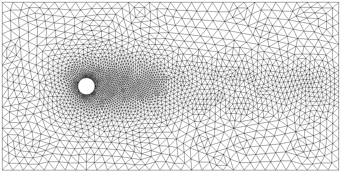
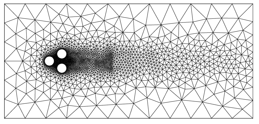
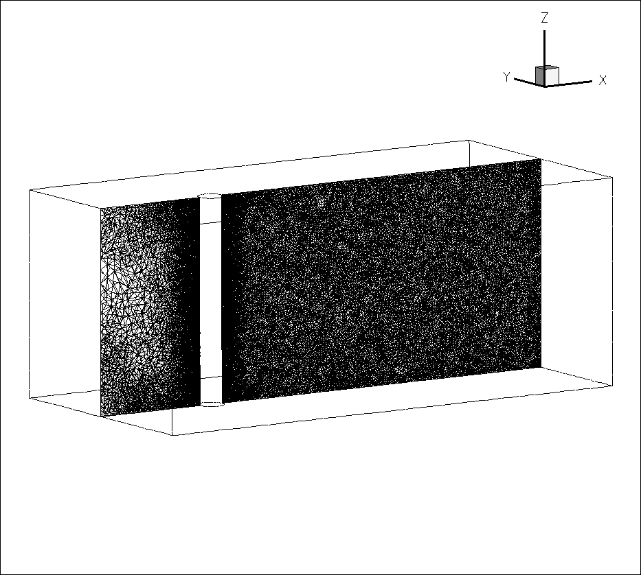
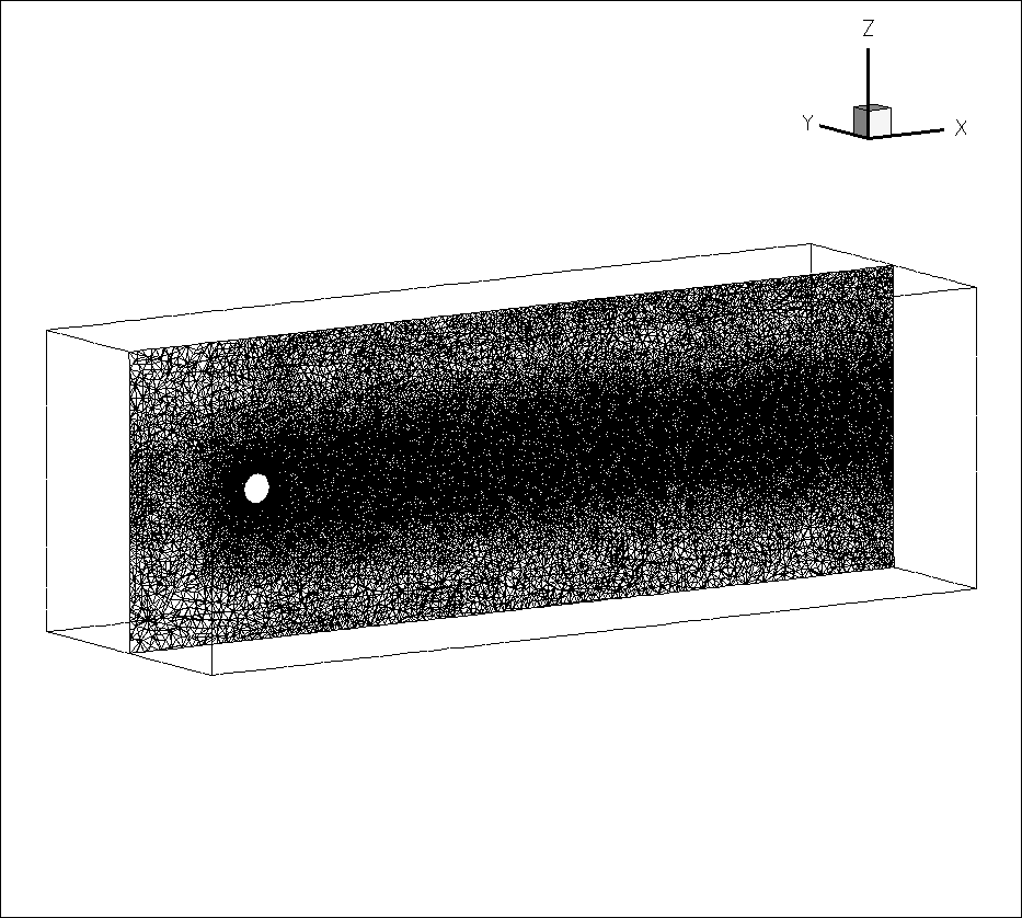
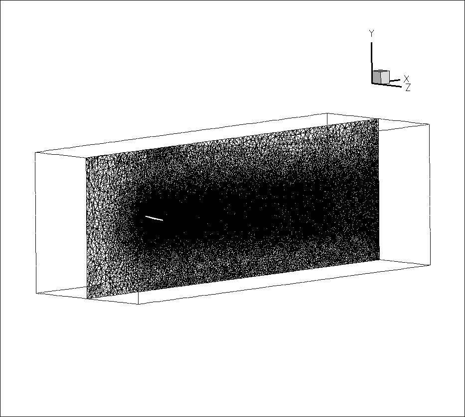
Figure 2: Grids used in 2D and 3D computations. The top row shows the 2D grids for the cylinder (left) and pinball configuration (right). The bottom row visualizes the 3D grids for the wall mounted cylinder (left), the sphere (middle) and the delta wing (right) in a representative plane.

2.7 Steady Navier-Stokes Solution

The first step in the solution of (5) is to determine the steady base solution of the Navier-Stokes equation (2). At smaller Reynolds numbers, the solution can be obtained directly with the steady version of (2) and an iterative method, like Newton-Raphson. At higher Reynolds numbers the computation can be difficult due to ill-conditioning of the system. One remedy is the use of Selective Frequency Damping (SFD) SFD . Simple unsteady computations with the low order time scheme and time step increasing during the computations gives also good approximation of the steady base solution.

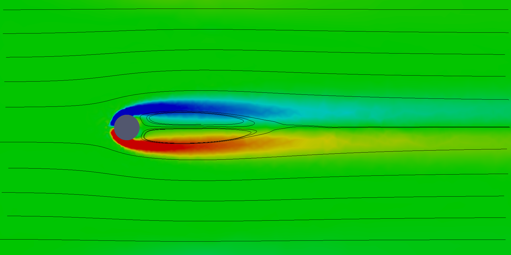
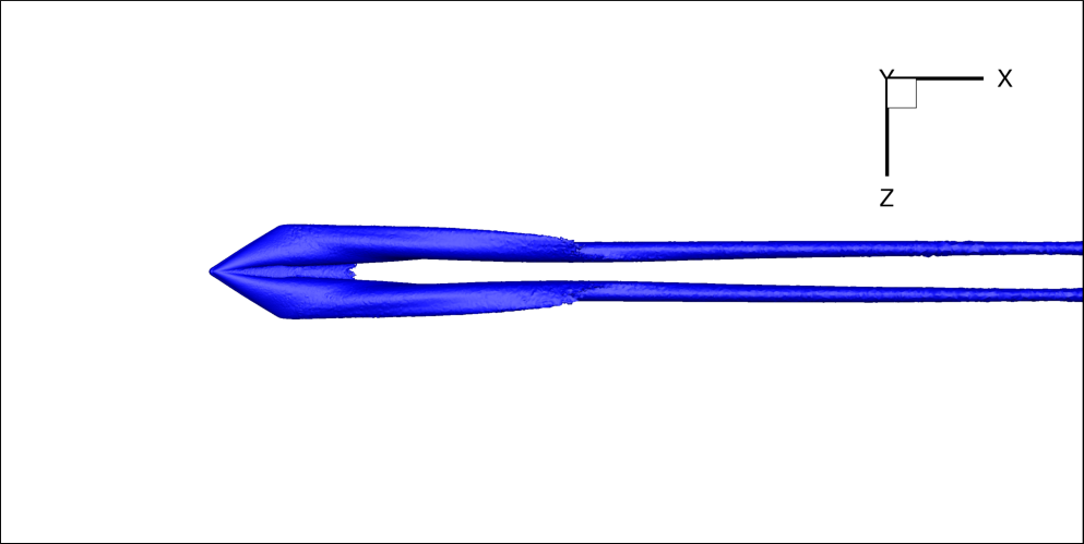
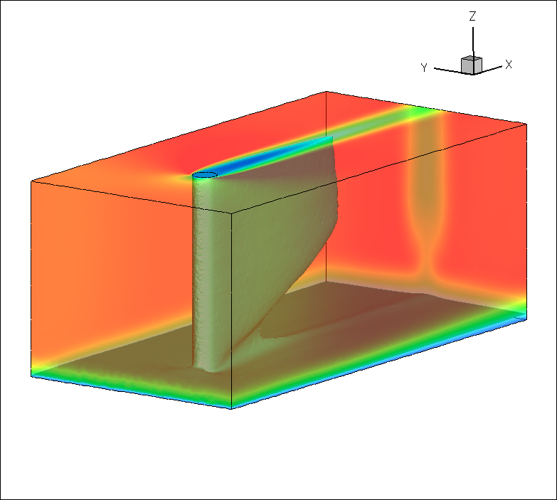
Figure 3: Steady Navier-Stokes solutions of the flow around a circular cylinder at $Re=100$ (top, vorticity field), a non-slender delta wing at $Re=1000$ (middle, velocity isosurface) and a wall-mounted cylinder at $Re=200$ (bottom, velocity isosurface with boundary values).

In Fig. 3, examples of steady base flows are shown for circular cylinder flow, the non-slender delta wing and the wall-mounted cylinder. In all these presented computations, we employ only the steady solution of the Navier-Stokes equations but the presented methodology is able to handle the flow dynamics around a mean flow as well.

3 Two-dimensional Flows

3.1 Wake Stabilization by High-frequency Rotation

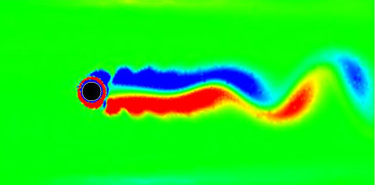
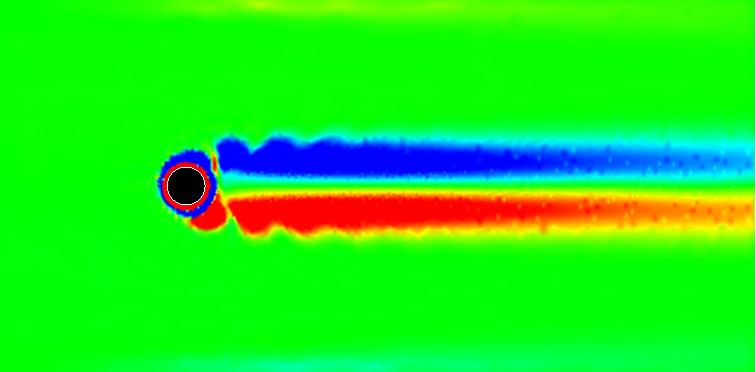
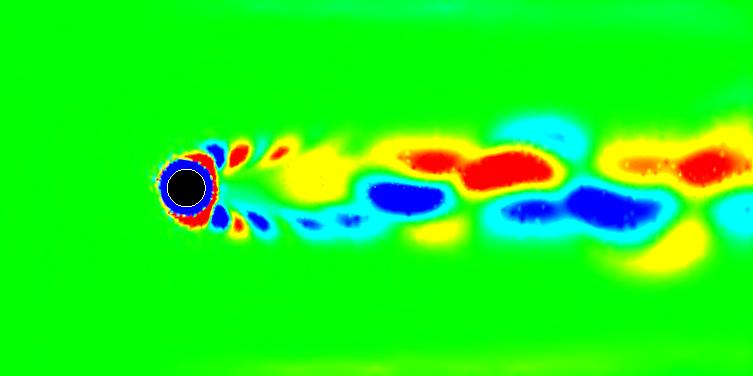
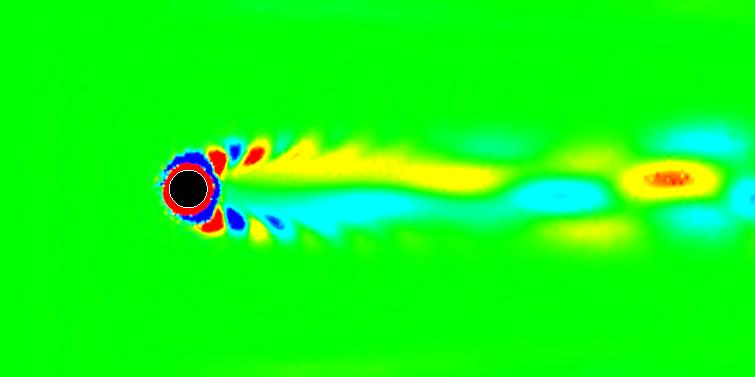
Figure 4: Wake of a cylinder with oscillatory rotation. The left (right) column visualizes the flow at $t=35$ ($t=200$). The top (bottom) row corresponds to the vorticity of the solution (disturbance).

As the motivation and illustration of the proposed methodology, we show the numerical experiment in stabilizing the von Kármán vortex street with the rotational oscillation of the cylinder at $Re=100$. The oscillation of the cylinder is chosen here to be $4.5$ times of the vortex shedding one. In Fig. 4, we show the effect of the applied control. The upper part of the figure shows the flow field at time instants $t=33$ and $t=200$ with initial actuation of the shear layer and the final, stabilized flow. The lower part shows the disturbance of the same time snapshot. The numerical experiments reproduce the water channel investigations of  Thiria2006jfm . With the frequency domain computations prior to the experiment there is a good opportunity to anticipate the stabilization scenario. The effect of oscillatory actuation of a circular cylinder flow is shown in Fig. 6 as the pure shear layer mode. What distinguishes this from Fig. 4 is exclusion of the von Kármán mode and its nonlinear interactions.

3.2 Cylinder Wake

We consider the unstable steady solution of the circular cylinder flow at $Re=100$. We show the effect of the symmetric disturbance triggered by a small $x$–axis motion of the cylinder in Fig. 5 and the antisymmetric one, by a small rotational oscillation of the cylinder in Fig. 6. The imaginary part of the shift, $\lambda_{Im}$ related to the frequency with $\lambda_{Im}=2\pi f$ is $4.2$, $3.2$, $2.2$, $1.2$, $0.87$ and $0.6$ respectively. The global stability analysis determines the von Kármán mode frequency $\lambda_{Im}$ for this configuration to be $0.87$. For the symmetric perturbation we obtain the symmetric pattern of the shear flow structures (counter-rotating pairs of vortices, symmetric about x–axis of the flow) for all frequencies except the von Kármán mode one. Rotation excites co-rotating structures in the shear layer, which merge into the von Kármán mode at $\lambda_{Im}=0.87$ and form more modes of this type for lower $\lambda_{Im}$.

It is also possible to use for actuation the volume force placed in the flow field. In Fig. 7 the actuation with the point volume force is demonstrated. Further experiments with the volume force are shown in Sect. 3.3.

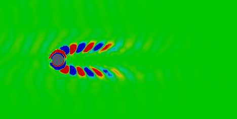
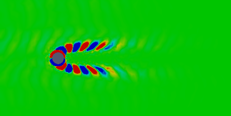
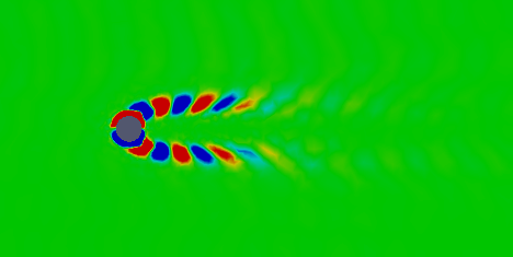
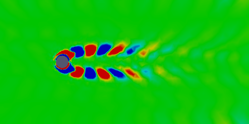
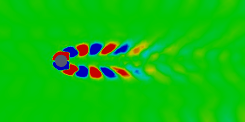
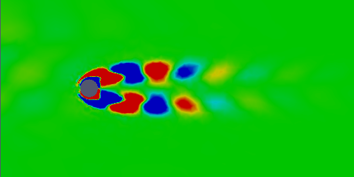
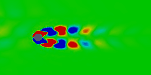
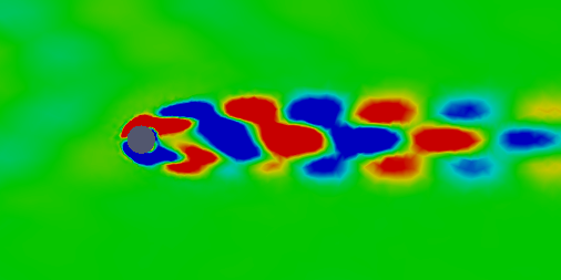
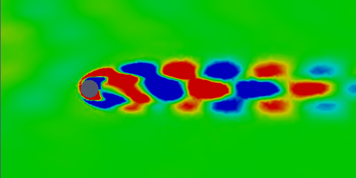
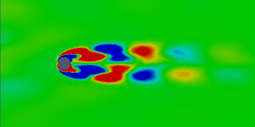
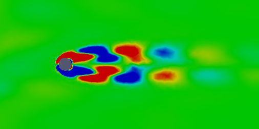
Figure 5: Modes for the circular cylinder wake at $Re=100$ and a symmetric disturbance. From top to bottom, $\lambda_{Im}$ is equal to $4.2$, $3.2$, $2.2$, $1.2$, $0.87$ and $0.6$. Real (left) and imaginary (right) vorticity fields are shown.

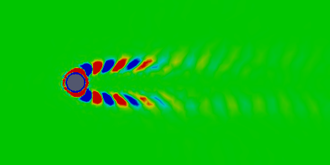
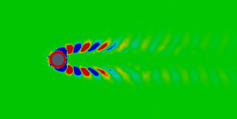
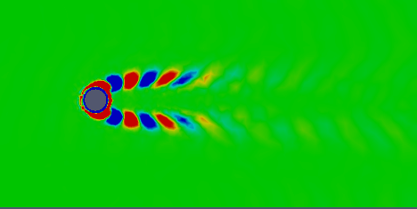
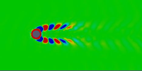
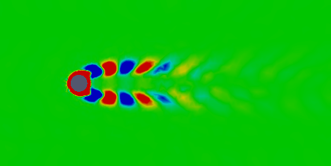
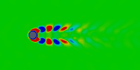
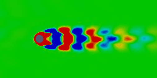
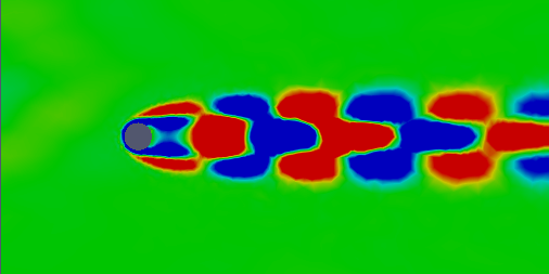
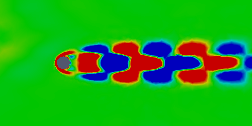
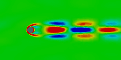
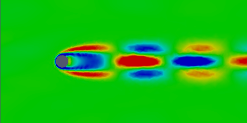
Figure 6: Modes for the circular cylinder wake at $Re=100$ and an oscillatory cylinder rotation. From top to bottom, $\lambda_{Im}$ is equal to $4.2$, $3.2$, $2.2$, $1.2$, $0.87$ and $0.6$. Real (left) and imaginary (right) vorticity fields are shown.

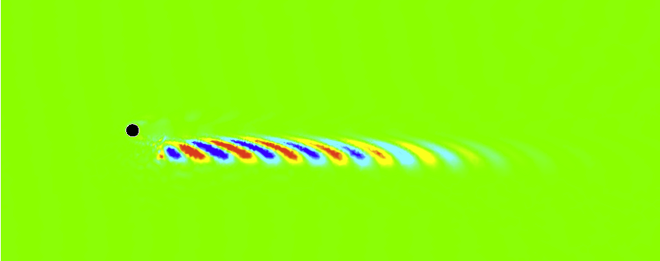
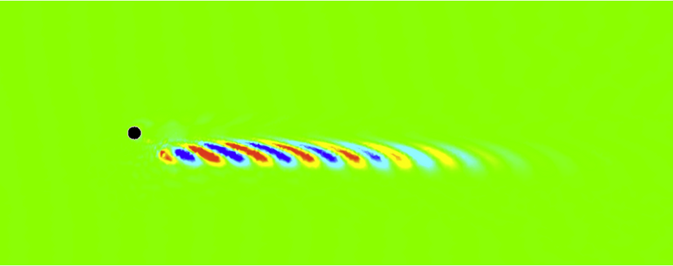
Figure 7: The effect of periodic forcing with a point volume force, $\lambda=0.13+i\,1.87$. Vorticity field shown.

3.3 Fluidic Pinball

The fluidic pinball is a set of three equal circular cylinders with radius $R$ placed parallel to each other in a viscous incompressible uniform flow at speed $U_{\infty}$. The cylinders can rotate at different speeds creating a variety of steady flow solutions and generating a kaleidoscope of vortical structures. The configuration is widely used for evaluation of flow controllers Cornejo2017limsi as this problem is challenging task for control methods comprising several frequency crosstalk mechanisms Noack2017put . The centers of the cylinders form an equilateral triangle with side length $3R$, symmetrically positioned with respect to the flow. The leftmost triangle vertex points upstream, while the rightmost side is orthogonal to the oncoming flow. The origin of the Cartesian coordinate system is placed in the middle of the top and bottom cylinder. The Reynolds number $Re_{D}$, based on the diameter of the single cylinder is $Re_{D}=100$.

To demonstrate the method we compute the steady solution with the upper cylinder rotating counterclockwise, the lower one rotating clockwise and the center cylinder also in clockwise direction—all with unit circumferential velocity, i.e. is the same as the velocity of oncoming flow. The flow-field for this configuration is depicted in Fig. 8. The global stability analysis finds the eigenvalue $\lambda=-0.0748+i\,0.466$ and the corresponding complex eigenvector depicted in Fig. 9. The subsequent two figures show modes which are found with the frequency domain approach for $\lambda=-0.1+i\,0.45$. In the Fig. 10 the forcing volume force is placed in the point $(-1,-1)$ while in the Fig. 11 at $(-1,1)$. Here and in the following examples we use a relatively large value of the actuation to enable visual identification of the actuation placement. The modes closely resemble the stability eigenmodes and in this case the placement of the actuation is not relevant for the resulting flow field. The effective control of the flow is related to actuation of the different frequencies and structures which interact with dominating ones lead us to a desired flow state of the fluid. To assess this type of actuation we place the actuator, represented by the value force at the point $(-1,-1)$ and obtain a clear response of the lower shear layer as depicted in Fig. 12. At the same time the actuator placed at the point $(-1,-1)$ (Fig. 13) splits its effect to both shear layers resulting in less active excitation. Both results are intuitive but the computations show the qualitative picture of possible action.

Figure 8: Steady Navier-Stokes solution for the fluidic pinball. Vorticity field and flow streamlines are shown.

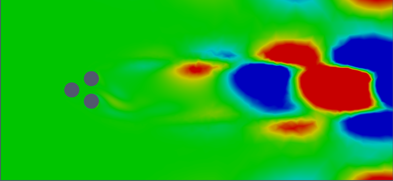
Figure 9: Dominating global stability eigenmode for $Re=100$. $\lambda=-0.0748+i\,0.466$. Vorticity field shown.

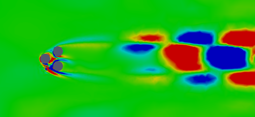
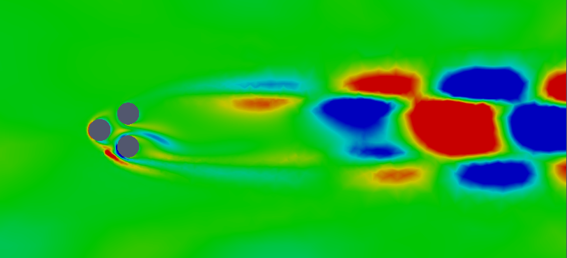
Figure 10: Von Kármán mode for $\lambda=-0.1+i0.45$, actuation at (-1,-1). Vorticity field shown.

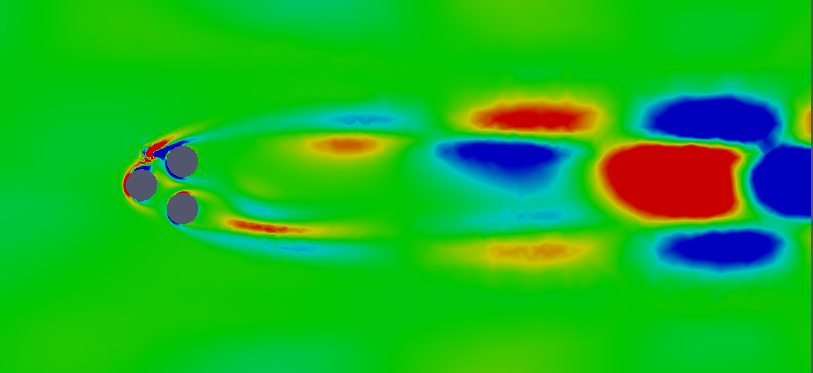
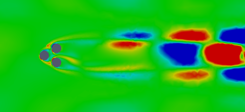
Figure 11: Von Kármán mode for $\lambda=-0.1+i0.45$, actuation at (1,1). Vorticity field shown.

Figure 12: Shear layer mode for $\lambda=0.2+i1.8$, actuation at (-1,-1). Vorticity field shown.

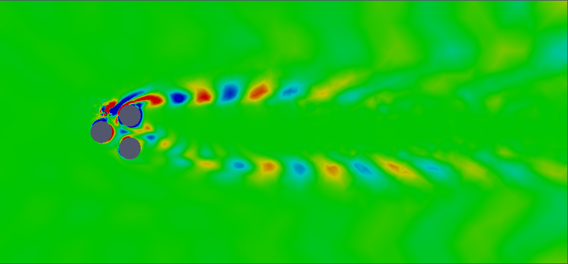
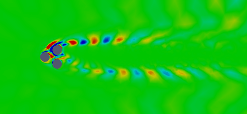
Figure 13: Shear layer mode for $\lambda=0.2+i1.8$, actuation at (1,1). Vorticity field shown.

4 Three-dimensional Flows

The pronounced complex pair of modes shown in Sect. 3 is obtained in relatively few iterations. This is in contrast to lengthy time integration and can be particularly attractive for 3D computations. We start the analysis with the academic example of a flow around a wall-mounted circular cylinder and of a sphere. In addition, we investigate a non–slender delta wing having an non-vanishing angle of attack (AoA).

4.1 Wall Mounted Cylinder

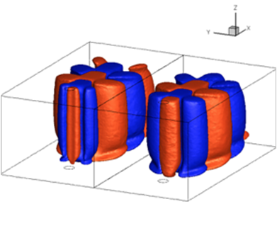
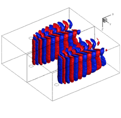
Figure 14: Flow around a wall-mounted circular cylinder at $Re=300$, $H=8D$. The left (right) figure shows the real and imaginary part of the von Kármán (shear-layer) mode. Both figures include vorticity isosurfaces (red -– negative, blue – positive).

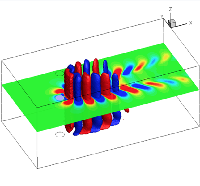
Figure 15: Close-up view of the real part of the shear-layer mode in Figure 14.

In Fig. 14 the 3D von Kármán and shear-layer mode is depicted for $H=8D$ and $Re=300$. Like for the two-dimensional cylinder wake, the real and imaginary part of the modes are shifted in phase. The bottom wall has a small effect on the dynamics.

In Fig. 15 the shear-layer mode is depicted in greater detail. The antisymmetric flow structures are visualized by iso-surface of $V_{1}$. There is mode deformation on the lower surface resulting from no-slip condition on the wall, different from the 2D cylinder flow in Sect. 2.

4.2 Sphere

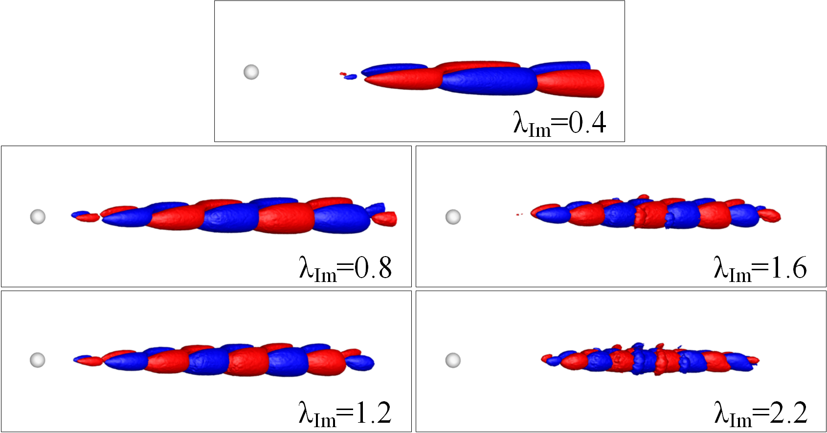
Figure 16: Sphere modes—Flow response to different frequencies of disturbance. Here, $Re=300$. The structures represent iso-surface of the streamwise velocity component (red -– negative, blue -– positive).

The sphere wake is a prototype of many aerodynamic bluff-body flows. Here, we present the structures building in the wake of a sphere at $Re=300$. In Fig. 16, the modes in the wake are present and growing at different axial location. The closest to the sphere are the modes having frequency closest to the shedding frequency, being the global stability eigenmodes. The frequency is also determining the axial dimension of spirally twisted structures.

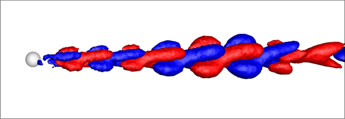
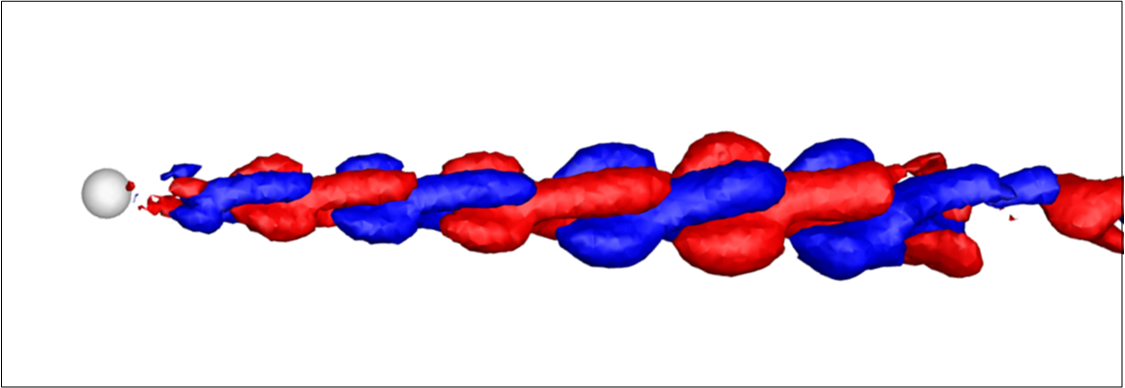
Figure 17: Sphere wake—DMD mode (real part–left, imaginary part–right) of the transient flow around a sphere at $Re=300$ near the fixed point (isosurfaces of streamwise velocity plotted, red -– negative, blue -– positive).

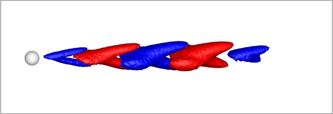
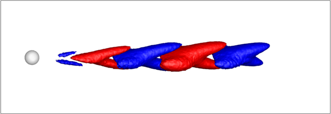
Figure 18: Sphere wake—Real and imaginary part of the of the frequency domain solution, $Re=300$, forcing at $\lambda_{Im}=0.785$ (isosurfaces of streamwise velocity plotted, red -– negative, blue -– positive).

In Figures 17 and 18, we show the Dynamic Mode Decomposition (DMD) modes for the shedding frequency and the ones obtained with the frequency domain computations. The similarities and differences of both sets of modes are clearly seen.

4.3 Delta Wing

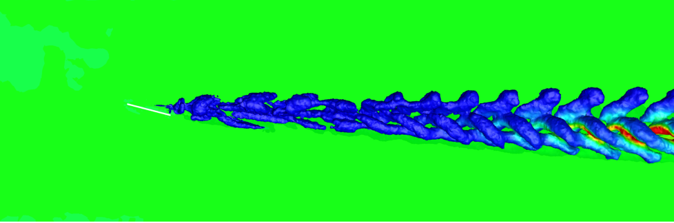
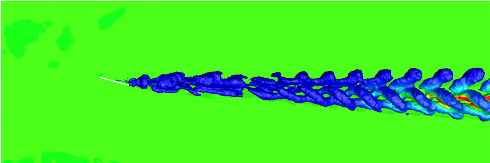
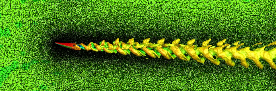
Figure 19: Non-slender delta wing ($65^{\circ}$) at $15^{\circ}$ AoA, $Re=500$. The flow is visualized with $\lambda_{2}$ iso-surfaces. Upper row: real and imaginary mode for dominating frequency. Lower row: visualization of the fully developed flow computed with the unsteady DNS solver.

The non-slender delta wing, having a non-vanishing angle of attack is close to a real-life configuration and very rich in flow phenomena. The steady solution, depicted in Fig. 3, shows a separation region behind the body and two vortical structures extending far downstream. The unsteady solution, even at relatively low Reynolds number, combines sphere-like vortex shedding interplay between vortices shed from the right and left part of the wing and a swirl around the vortex cores. Modes for such a complex flow are of particular interest.

In Fig. 19, the real and imaginary part of the dominating mode are shown. The flow is obtained for a $65^{\circ}$ triangular wing at $15^{\circ}$ angle of attack. The Reynolds number for this flow is $Re=500$. Because of the complexity of the flow, $\lambda_{2}$ surfaces are depicted. In the bottom part of the figure the snapshot of an unsteady DNS simulation is depicted also with $\lambda_{2}$ surfaces. The dominant structures are present already in the linear solution of frequency domain formulation.

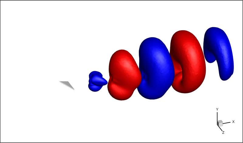
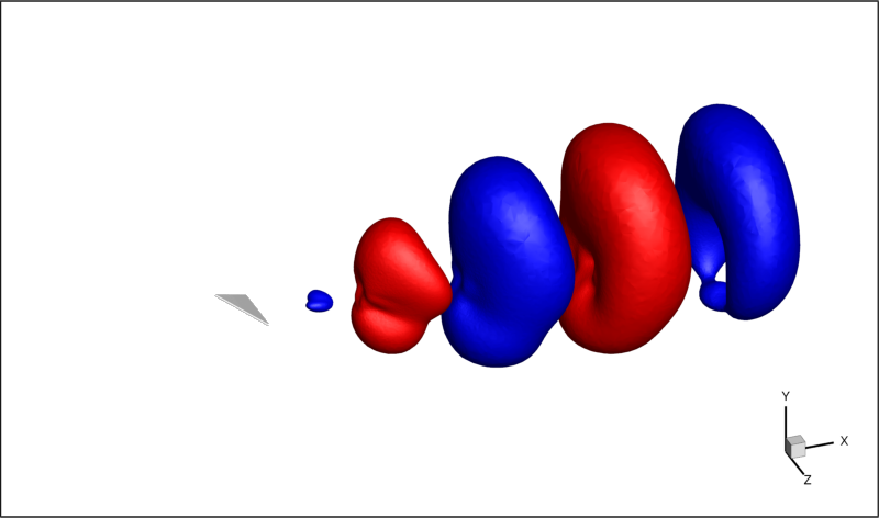
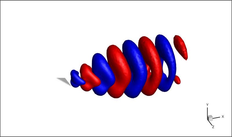
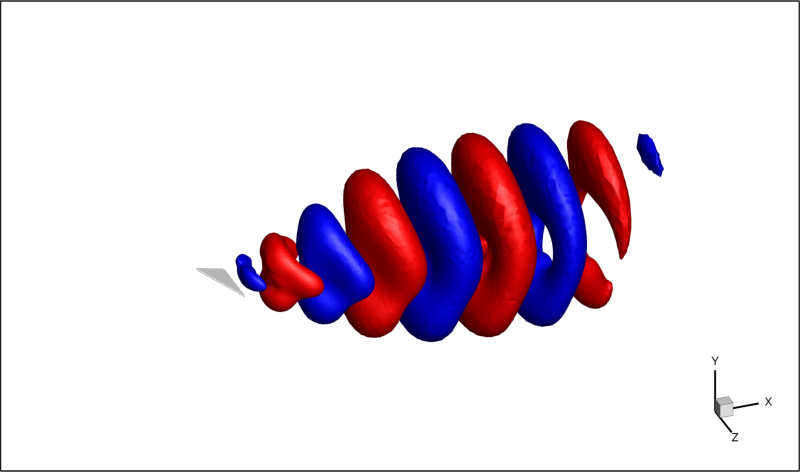
Figure 20: Non-slender delta wing ($65^{\circ}$), AoA$=30^{\circ}$, $Re=1000$. Complex modes (real part –- left, imaginary part –- right) computed in the frequency domain with forcing frequencies $\lambda_{Im}=0.75$ (top) and $\lambda_{Im}=1.5$ (bottom). Isosurfaces of the velocity streamwise component are shown (negative -– red, positive -– blue).

Further figures show the results for the angle of attack of $30^{\circ}$, with iso-lines of streamwise velocity for $Re=1000$. For both investigated frequencies ($\lambda_{Im}=0.75$ and $\lambda_{Im}=1.5$) the modes have shedding character.

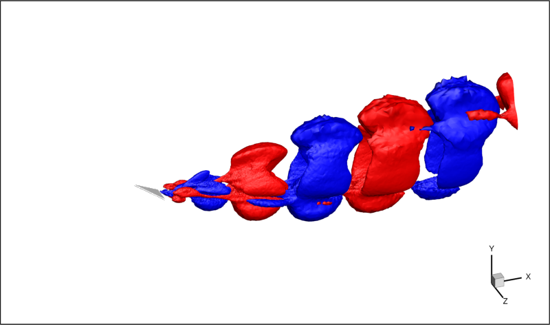
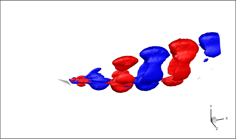
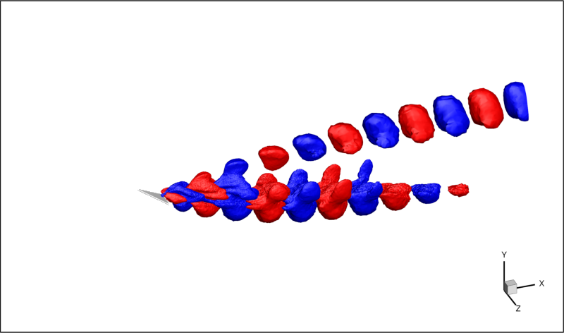
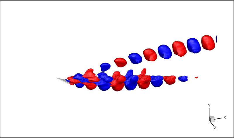
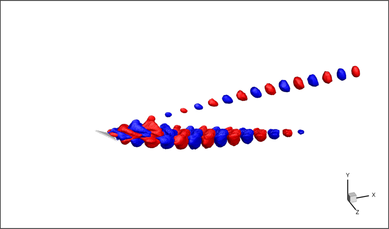
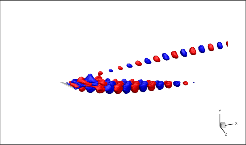
Figure 21: Delta wing ($35^{\circ}$), AoA$=30^{\circ},$ $Re=1000$. Complex modes (real part –- left, imaginary part -– right) computed in the frequency domain. Here $\lambda_{Im}=0.75$ (top), $\lambda_{Im}=1.5$ (middle), $\lambda_{Im}=2.5$ (bottom). Isosurfaces of the velocity streamwise component are shown (negative -– red, positive -– blue).

For a $35^{\circ}$ wing at the same Reynolds number ($Re=1000$) and angle of attack $30^{\circ}$ we have shedding mode and higher order modes, extending along the steady solution vortex cores (Fig. 21).

5 Nonlinear First-Principle Reduced-Order Modeling of Periodic Wake Actuation

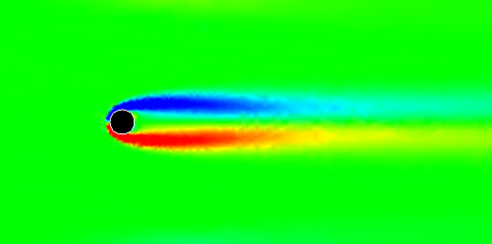
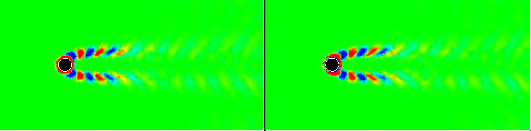
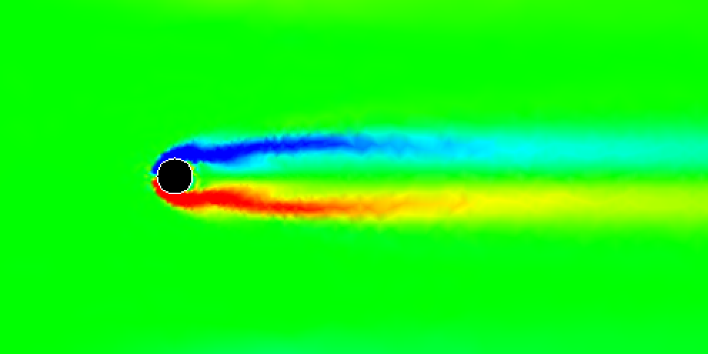
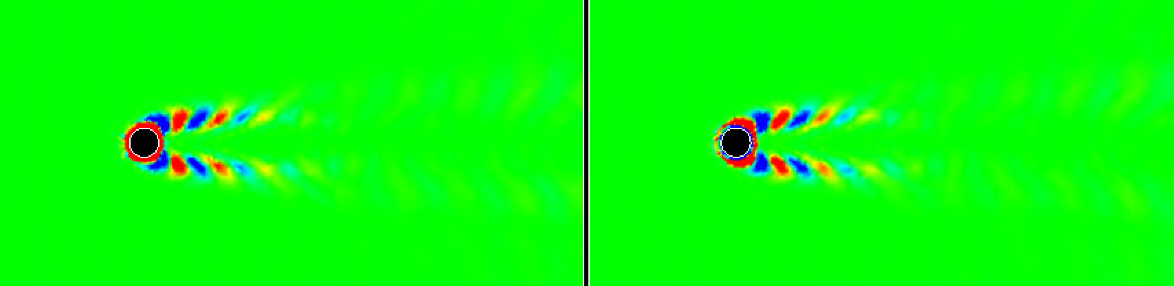
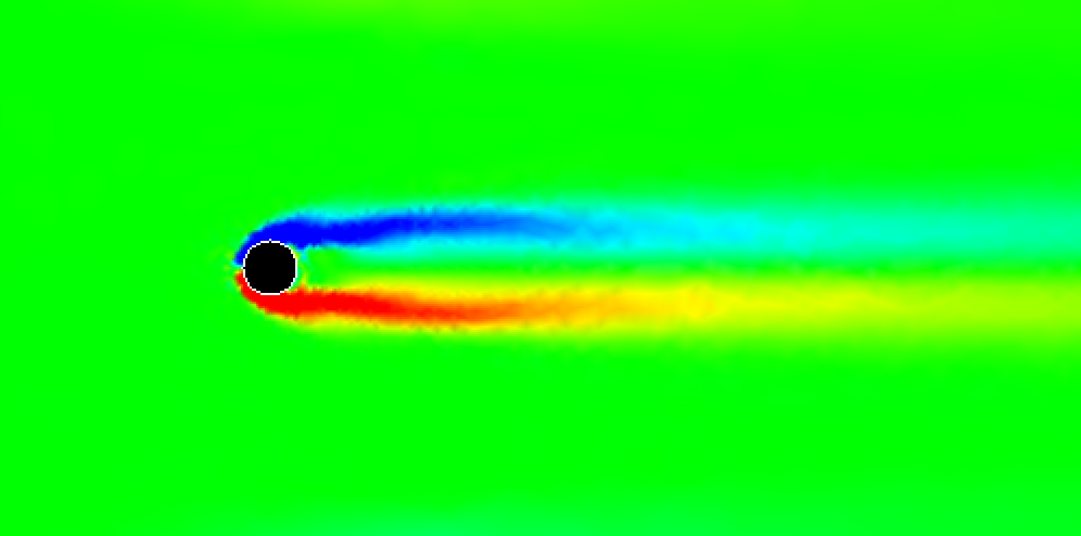
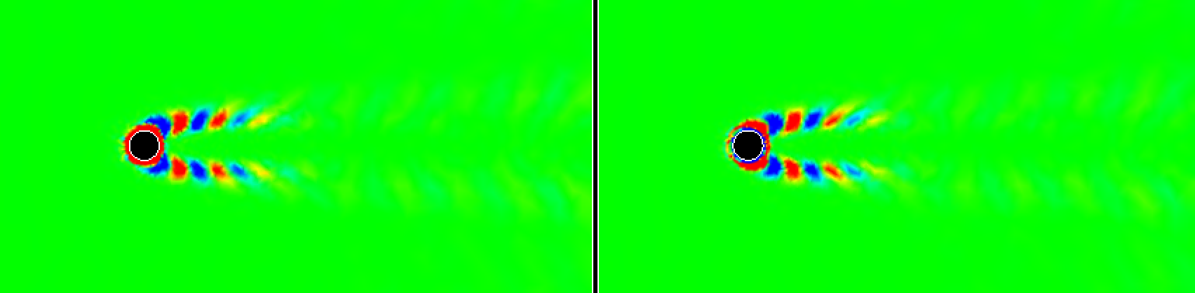
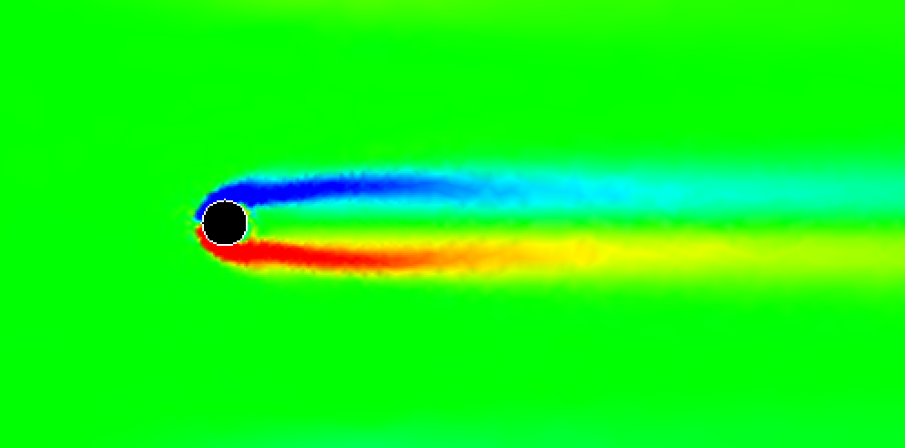
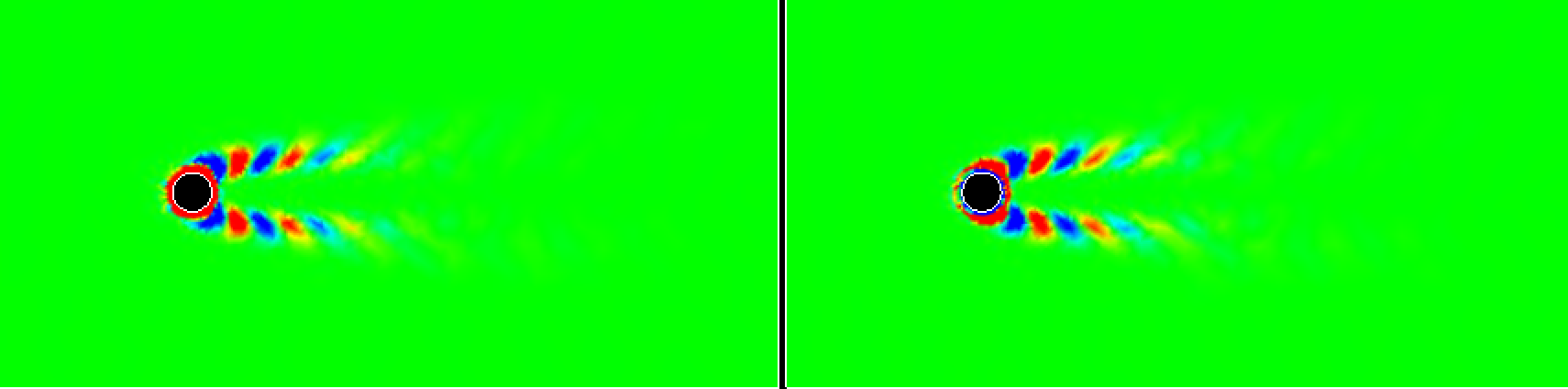
Figure 22: Iterations of the nonlinear model with a physical actuation mode. Actuation with oscillatory rotation ($\lambda_{Im}=4.0$) of a circular cylinder at $Re=100$. From top to bottom: Vorticity of the mean flow as obtained from Reynolds equation (left) with corresponding actuation modes (real and imaginary part, right) in iteration 1, 2, 3 and 10.

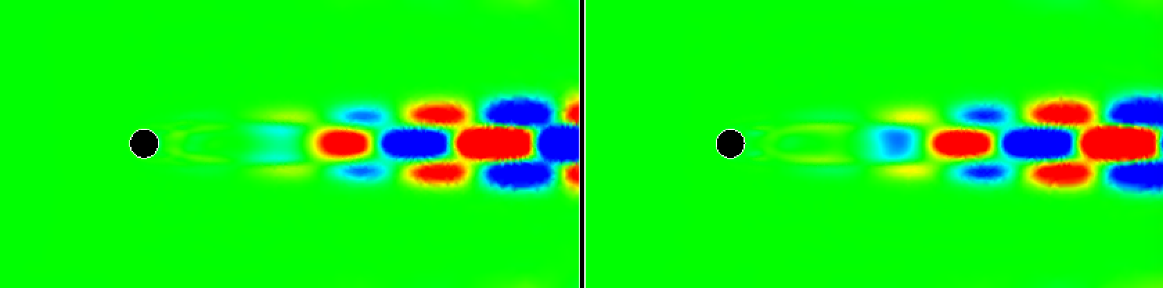
Figure 23: Eigenmodes (real part: left, imaginary part: right) associated with the mean flow of the nonlinear actuation model displayed in Fig. 22. From top to bottom: the vorticity at iteration 1, 3 and 10.

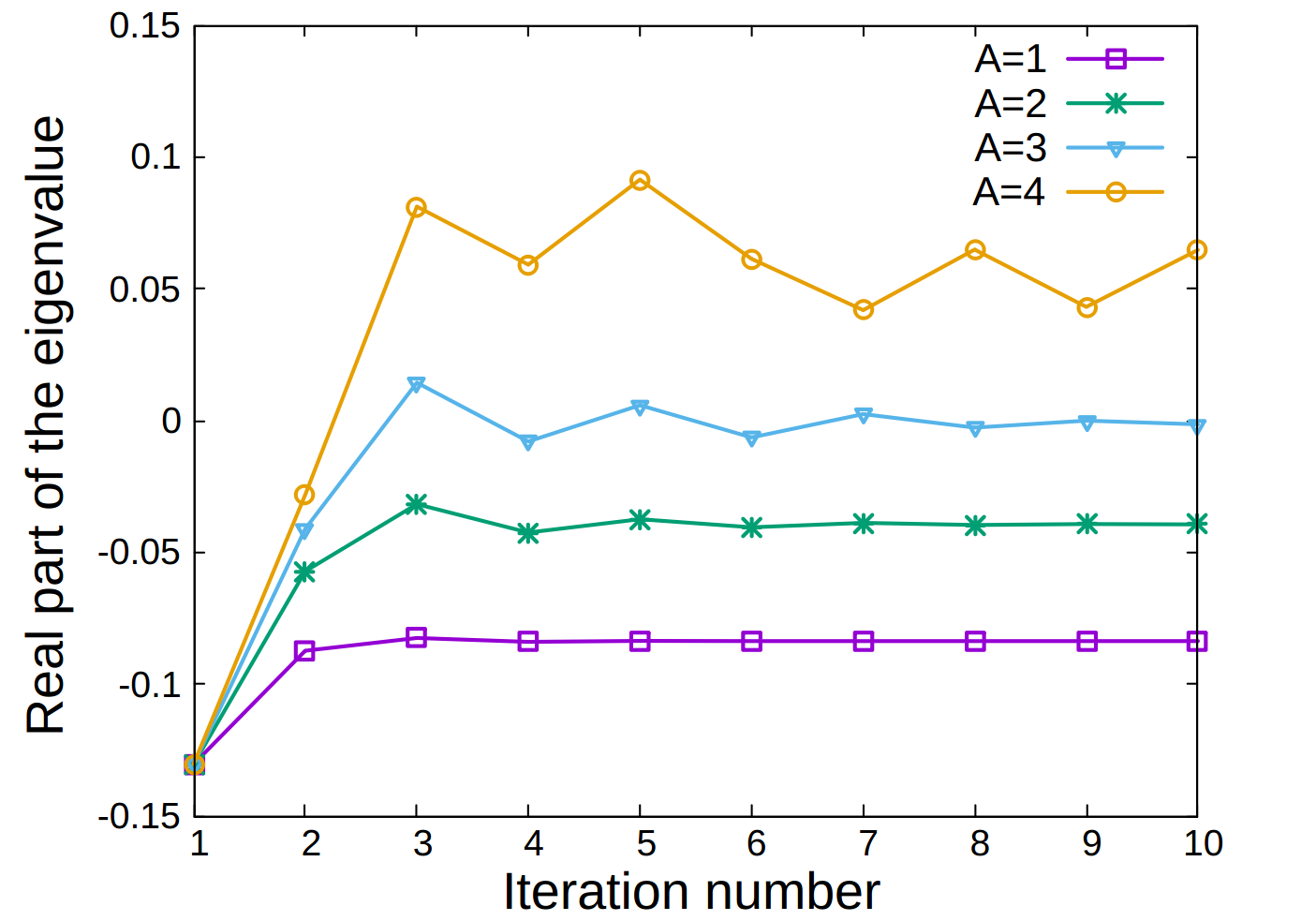
Figure 24: Growth rates of the eigenmodes depicted in Fig. 23 in dependency of the iteration number.

In this section, we demonstrate how nonlinear actuation performance can be predicted using the unstable periodically forced Navier-Stokes solution computed in the previous sections. Starting point is the high-frequency actuation of a circular cylinder wake at $Re=100$ of Sect. 3.1. An experiment Thiria2006jfm demonstrated that this actuation can stabilize the cylinder wake via nonlinear frequency crosstalk mechanisms. In the following, this nonlinear actuation effect is resolved in a first-principle reduced-order model based on mean-field considerations.

Most flow control experiments rely on the nonlinear interaction between the mean flow and unsteady fluctuation Tadmor1513 . Fluctuations change the mean flow via the Reynolds stress. Inversely, mean flow variations change also the stability properties of the fluctuations. This frequency crosstalk mechanism is exploited in a stabilization of the target instability with low- and high-frequency actuation Brunton2015amr . A linearly stable solution of the Reynolds equation implies that the actuated flow structures have successfully stabilized the flow.

The stabilizing effect of periodic actuation is described by the Reynolds equation

$$\bar{V}_{i,j}\bar{V}_{j}+\bar{P}_{,i}-\frac{1}{Re}{\bar{V}_{i,jj}}-\frac{1}{2}A^{2}\nabla\cdot[\vec{V}_{real}\otimes\vec{V}_{real}+\vec{V}_{imag}\otimes\vec{V}_{imag}]=0$$ (30)

Here $\bar{V}_{i}$ and $\bar{P}$ are the mean field values, $\vec{V}_{real}$ and $\vec{V}_{imag}$ are the real and imaginary parts of the actuation mode computed with the procedure described in Sect. 3.2. and $A$ is the amplitude of the actuation. It should be noted that (30) only includes the Reynolds stress of the actuation mode. Thus, (30) implies a successful flow stabilization which can a posteriori be validated with the stability of computed mean flow.

The Reynolds equation (30) depends on the actuation mode $\vec{V}$ as sole contribution to the Reynolds stress. Inversely, the actuation mode depends on the base flow as evidenced by the disturbance equation (5). This reciprocal dependency between mean flow and actuation mode is resolved by an iteration algorithm. In the first step, the steady Navier-Stokes solution is computed and taken as base flow for (5) and subsequent eigenproblems for the actuation mode. In the second step, a base flow is updated with the Reynolds equation (30) using the actuation mode. In addition, the actuation mode is re-computed with the new base flow. These iterations are continued until convergence. In each iteration, a global stability analysis may assess the suppression of the target instability.

The iterative procedure is depicted for forcing $\lambda_{Im}=4.0$ encoded in the imaginary part of the eigenvalue and the amplitude of oscillation $A=3$. Figs. 22, 23 and 24 show the convergence of the base flow, the actuation mode, the most unstable eigenmode and its corresponding growth-rate.

We start with the steady flow solution at $Re=100$. The vorticity of the flow is depicted in the first row of Fig. 22 (left). The global stability analysis of this flow field yields von Kármán vortex shedding (Fig. 23, top row) with negative $\lambda_{Re}$ (Fig. 24) indicating that the base flow is unstable. The flow response to a stabilizing high-frequency rotary oscillation is resolved by an actuation mode, following an earlier numerical study. With the technique presented in Sect. 3.2, we obtain the complex actuation mode shown in the top row of Fig. 22 (right).

In the second iteration, the actuation mode is employed in the Reynolds equation (30) to derive the corresponding mean flow (Fig. 22, 2nd row, left). This mean flow is used to revise the actuation mode (Fig. 22, 2nd row, right).

The process converges in about ten iterations yielding the final mean flow field and associated actuation mode (Fig. 22, last row). The stability of the base flow is assessed via a global stability analysis. If the growth rate is non-positive, a stabilization of the flow is achieved.

In Fig. 24, the evolution of the growth rate is depicted at different amplitudes of the actuation amplitude $A$, including a strongly, marginal and partially stabilizing level. In Fig. 23, the corresponding global modes of the mean flow are illustrated for subsequent iterations, showing the stabilization of the flow. The center of vorticity moves towards the outflow, indicating that actuation effectively stabilizes the near-wake and a marginally stable von Kármán mode fluctuation may only exists far downstream.

The analysis is consistent with nonlinear Navier-Stokes simulations and serves as the demonstration of capability of the method. The nonlinear first-principle reduced-order model from the iterative procedure may resolve the performance of different actuation types, frequencies and amplitudes. Arbitrary kinds of the actuation can be tested using the fact that the equation (8) and the resulting discrete one (11) are linear and we can superpose their solutions. At the same time we can investigate also the effect of actuator placement. We emphasize that the resulting reduced-order model is consistent with generalized mean-field theory but forced and unstable harmonic components are fully resolved in a first-principle Navier-Stokes discretization. In contrast, the generalized mean-field model of Luchtenburg2009jfm employs empirical shedding and actuation modes, i.e. is only consistent with the one actuation for the simulation data.

6 Conclusions

Several applications of frequency domain computations, employing complex shift have been presented. The method is very similar to global (fully two–dimensional or fully three–dimensional) stability analysis, yet yields a broader range of results. First, the most amplified global eigenmodes are reproduced. Second, we compute unstable Navier-Stokes solutions featuring the periodic flow responses at any given frequency, potentially corresponding to damped eigenmodes. The latter addresses a challenge of computational stability analysis: While the most amplified eigenmode is easily distilled by a power method, the more damped modes live ’under the radar’ of many iterative solvers for eigenmodes.

The frequency domain computation has a straight-forward mathematical formulation. The numerical realization and the algorithm behavior demand careful handling of boundary conditions, meshing and numerical schemes. The similarity of our computations to the methods used in computational aeroacoustics suggests careful use of sponge-layer boundaries, high-order schemes and sensitivity to spurious oscillatory solutions. There is much less experience and techniques for these computations as computations in frequency domain are far more rare in computational fluid dynamics than regular time-stepping approaches. Shifted problems are different from singular ones but still the numerical properties of the system are less predictable than for the regular CFD ones.

The proposed method has evident applications in active flow control. It could be used to explore excitable coherent structures which mitigate the target instability via nonlinear frequency crosstalk Brunton2015amr , as it is much easier to excite than to damp an eigenmode. The presented nonlinear first-principle reduced-order model of wake stabilization with high-frequency forcing underlines this perspective.

The methodology can be significantly extended and has many more applications. For example, the adjoint analysis in the spirit of Luccini Luchini2014 is possible with minor modification of the program. Another application is the use of mean flow as the base solution, as pioneered by Michalke Michalke1965jfm and continued by Barkley Barkley2006ep . Another direction is the exploration of the rich nonlinear dynamics from interactions between eigenmodes Noack2008jnet . These are only a few directions of future directions of research.

The presented results are far from being a fool-proof methodology for computation of eigenmodes but rather a start of a highly promising avenue towards physical flow expansions, nonlinear first-principle Galerkin models and control applications—even for strongly nonlinear frequency crosstalk.

- (1) L.D. Landau. On the problem of turbulence. C.R. Acad. Sci. USSR, 44:311–314, 1944.
- (2) E. Hopf. A mathematical example displaying features of turbulence. Commun. Pure & Appl. Math., 1:303–322, 1948.
- (3) M.J. Feigenbaum. Quantitative universality for a class of nonlinear transformations. J. Stat. Phys., 19:25–52, 1978.
- (4) D. Ruelle and F. Takens. On the nature of turbulence. Comm. Math. Phys., 20:167–192, 1971.
- (5) S. Newhouse, D. Ruelle, and F. Takens. Occurence of strange Axiom-A attractors near quasiperiodic flow on , . Comm. Math. Phys., 64:35, 1978.
- (6) Y. Pomeaou and P. Manneville. Intermittent transition to turbulence in dissipative dynamical systems. Commun. Math. Phys., 74:189–197, 1980.
- (7) E. Åkervik, J. Hœpffner, U. Ehrenstein, and D. S. Henningson. Optimal growth, model reduction and control in separated boundary-layer flow using global eigenmodes. J. Fluid Mech., 579:305–314, 2007.
- (8) B. R. Noack, K. Afanasiev, M. Morzyński, G. Tadmor, and F. Thiele. A hierarchy of low-dimensional models for the transient and post-transient cylinder wake. J. Fluid Mech., 497:335–363, 2003.
- (9) C. E. Grosch and H. Salwen. The continuous spectrum of the Orr-Sommerfeld equation. Part I. The spectrum and the eigenfunctions. J. Fluid Mech., 87:33–54, 1978.
- (10) H. Salwen and C. E. Grosch. The continuous spectrum of the Orr-Sommerfeld equation. Part 2. Eigenfunction expansions. J. Fluid Mech., 104:445–465, 1981.
- (11) K. Taira, S. L. Brunton, S. Dawson, C. W. Rowley, T. Colonius, B. J. McKeon, O. T. Schmidt, S. Gordeyew, V. Theofilis, and L. S. Ukeiley. Modal analysis of fluid flows: An overview. arXiv, (1702.01453 [physics.fui-dyn]), 2018.
- (12) V. Theofilis. Advances in global linear instability analysis of nonparallel and three-dimensional flows. Prog. Aerosp. Sci., 39(4):249–315, 2003.
- (13) V. Theofilis. Global linear instability. Ann. Rev. Fluid Mech., 43:319–352, 2011.
- (14) D. Wolter, M. Morzyński, H. Schütz, and F. Thiele. Numerische Untersuchungen zur Stabilität der Kreiszylinderumströmung. Z. Angew. Math. Mech, 69:T601–T604, 1989.
- (15) M. Morzyński, K. Afanasiev, and F. Thiele. Solution of the eigenvalue problems resulting from global non-parallel flow stability analysis. Computer Methods in Applied Mechanics and Engineering, 169(1):161 – 176, 1999.
- (16) M. Morzyński and F. Thiele. 3D FEM Global Stability Analysis of viscous flow. In Lecture Notes in Computer Science, Parallel Processing and Applied Mathematics, volume 4967, pages 1293–1302. Springer-Verlag, 2008.
- (17) F. Gómez, J. M. Pérez, H. M. Blackburn, and V. Theofilis. On the use of matrix-free shift-invert strategies for global flow instability analysis. Aerosp. Sci. Techn., 44:69–76, 2015.
- (18) Q. Liu, F. Gómez, Pérez J. M., and V. Theofilis. Instability and sensitivity analysis of flows using openfoam®. Chin. J. Aeronautics, 29(2):316 – 325, 2016.
- (19) O. Semeraro, S. Bagheri, L. Brandt, and D. S. Henningson. Feedback control of three-dimensional optimal disturbances using reduced-order models. J. Fluid Mech., 677:63–102, 2011.
- (20) X. Garnaud, L. Lesshafft, P. J. Schmid, and P. Huerre. The preferred mode of incompressible jets: linear frequency response analysis. J. Fluid Mech., 716:189–202, 2013.
- (21) E. Åkervik, J. Hœpffner, U. Ehrenstein, and D. S. Henningson. Optimal growth, model reduction and control in a separated boundary-layer flow using global eigenmodes. J. Fluid Mech., 579:305–314, 2007.
- (22) J. M. Chomaz. Global instabilities in spatially developing flows: non-normality and nonlinearity. Annu. Rev. Fluid Mech., 37:357–392, 2005.
- (23) Z. Q. Qu. Model Order Reduction Techniques with Applications in Finite Element Analysis. Springer Science & Business Media, 2013.
- (24) E. L. Wilson, M. W. Yuan, and J. M. Dickens. Dynamic analysis by direct superposition of Ritz vectors. Earthquake Engineering & Structural Dynamics, 10(6):813–821, 1982.
- (25) C. Taylor and P. Hood. A numerical solution of the Navier-Stokes equations using the finite element technique. Comput. & Fluids, 1(1):73 – 100, 1973.
- (26) B. R. Noack and M. Morzyński. The fluidic pinball — a toolkit for multiple-input multiple-output flow control (version 1.0). Technical Report 02/2017, Chair of Virtual Engineering, Poznan University of Technology, Poland, 2017.
- (27) G. Y. Cornejo Maceda. Machine learning control applied to wake stabilization. M2 Master of Science Internship Report, LIMSI and ENSAM, Paris, France, 2017.
- (28) E. Åkervik, L. Brandt, D. S. Henningson, J. Hœpffner, O. Marxen, and P. Schlatter. Steady solutions of the Navier-Stokes equations by selective frequency damping. Physics of fluids, 18(6):068102, 2006.
- (29) B. Thiria, S. Goujon-Durand, and J. E. Wesfreid. The wake of a cylinder performing rotary oscillations. J. Fluid Mech., 560:123–147, 2006.
- (30) G. Tadmor, O. Lehmann, B. R. Noack, L. Cordier, J. Delville, J. P. Bonnet, and M. Morzyński. Reduced-order models for closed-loop wake control. Philosophical Transactions of the Royal Society of London A: Mathematical, Physical and Engineering Sciences, 369(1940):1513–1524, 2011.
- (31) S. L. Brunton and B. R. Noack. Closed-loop turbulence control: Progress and challenges. Appl. Mech. Rev., 67(5):050801:01–48, 2015.
- (32) Luchtenburg, D. M., Günter, B., Noack, B. R., King, R. and Tadmor, G. A generalized mean-field model of the natural and actuated flows around a high-lift configuration. J. Fluid Mech., 623:283–316, 2009.
- (33) P. Luchini and A. Bottaro. Adjoint equations in stability analysis. Ann. Rev. Fluid Mech., 46(1):493–517, 2014.
- (34) A. Michalke. On spatially growing disturbances in an inviscid shear layer. J. Fluid Mech., 23:521–561, 1965.
- (35) D. Barkley. Linear analysis of the cylinder wake mean flow. Europhysics Lett., 75:750–756, 2006.
- (36) B. R. Noack, M. Schlegel, B. Ahlborn, G. Mutschke, M. Morzyński, P. Comte, and G. Tadmor. A finite-time thermodynamics of unsteady fluid flows. J. Non-Equilibr. Thermodyn., 33:103–148, 2008.