Universality and Regge-like spectroscopy for orbitally-excited light mesons

Abstract

A new Regge-like mass relation for excited light mesons is presented in relativized quark model which supports an universality that the quark mass dependence of the light meson spectroscopy is suppressed significantly and the confining parameter is nearly family independent. It is obtained by using auxiliary field method and quasi-linearizing the solution to the mass relation solved from the model. The resulted mass predictions are in good agreement with the observed masses for the orbitally-excited trajectory family of $\pi/b$, $\rho/a$, $\eta/h$, $\omega/f$, $K^{\ast}$ and $\phi/f^{\prime}$. A semiclassical argument is given that the inverse slopes on the radial and angular-momentum Regge trajectories are equal in the massless limit of quarks.

I Introduction

The dynamics behind the formation of light hadrons still remains to be unclear four decades after the discovery of the theory of strong interaction, the quantum chromodynamics (QCD). In the case of the light mesons (which we shall discuss in this work) that composed of light quarks ($n\equiv(u,d),s$), the most lowest state are well established (with some exceptions, the $0^{++}$ scalar mesons etc.), while the excited states in the range $M>2GeV$ are less understood. Despite difficulties in solving QCD exactly, it is expected that properties and decay of light mesons will shed light on understanding of QCD at low energy. Recently, advances in experiment Patrignani:C16 , with light mesons generated in copious amounts, make it possible to address such issues as whether nonconventional states (exotics) exist in the light sector of hadrons. For instance, $a_{0}(980)$ and $f_{0}(980)$ were expected to be exotic WeinsteinI:1982 ; WeinsteinI:1983 . However, it is fair to say that we may not truly understand the spectrum of light mesons before we understand the excitations of the lowest mass mesons. Further, the light-meson spectrum has become important not merely for the intrinsic understanding of these states, but also as a prerequisite for exploring exotic states (see GodfreyN:P1999 ; AmslerT:RP04 for a review).

On the other hand, the observed spectrum of light mesons manifests themselves in almost universal pattern: they populate approximately linear Regge trajectories ChewF:61 , almost parallel between trajectories AnisovichAS:PRD00 ; MasjuanAB:D12 . This universal pattern of the hadron spectrum strongly hints that the formation dynamics of light mesons is more or less universal by itself in the sense that their spectrum are almost independent of the quark favors, as QCD is. Great success has been achieved in building dynamical quark models to describe the whole meson spectrum in an universal way (see, RujulaGG:D75 ; KangS:D75 ; BasdevantB:C85 ; GodfreyIsgur:85 ; EbertFG:D09 for instance) and argument was given Olsson:D1997 that universality can arise from the relativistic effects and the confinement dynamics. In the high excitation spectrum, however, this feature remains to be understood yet.

For light hadrons, a remarkable feature of Regge trajectory is that the slope $\alpha^{\prime}$ in the Chew-Frautschi relation, $L=\alpha^{\prime}M^{2}+\alpha(0)$, where $L$ is the angular momentum of the hadron state and $M$ its mass, depends weakly on the flavor content of the states lying on the corresponding trajectory. The Regge slope $\alpha^{\prime}$ varies slightly from trajectory to trajectory, by less than $10\%$ for nonstrange mesons AnisovichAS:PRD00 ; MasjuanAB:D12 ; Sharov:13 ; SonnenscheinW:JHEP14 , and the linearity of trajectories are commonly assumed. When strangeness involved, the situation becomes slightly involved. Nonlinearity in Regge trajectories was suggested BrisudovaBG:00 and the correction to the linear trajectory are explored in Refs. JohnsonN:PRD79 ; Afonin:B03 and Ref. SonnenscheinW:JHEP14 , for instance. It is then of important to examine carefully the properties of Regge trajectory with enriched experimental data of the light mesons. The knowledge of Regge trajectories is also valuable in the recombination and fragmentation models for hadrons transition in the scattering region ($t<0$) Collons:77 .

Purpose of this work is to explore the universality high in the excited spectrum of the light mesons using relativistic quark model combined with auxiliary field method. We propose a new Regge-like mass relation for the orbitally-excited light mesons which supports a universality that the quark mass dependence of the light meson spectroscopy is suppressed. The obtained mass relation is tested against the observed masses of mesons considered. It is found that the parameters in the relation are roughly universal except the vacuum constant. A explicit expression for the Regge slope and intercept was obtained and compared to the results extracted from the other analysis of the meson family of $\pi/b$, $\rho/a$, $\eta/h$ and $\omega/f$ in the ($L$,$M^{2}$) planes or predictions in the literatures. Suggestion is made that the members of the $\eta/h$ trajectory may contain components of exotics.

We also discuss the implications of our results in comparison with that in the string (flux-tube) picture of mesons Nambu:D74 ; Goto:71 and that in other quark models. By the way, semiclassical argument is given that the slopes on the radial and angular-momentum Regge trajectories are equal in the massless limit of quarks, as suggested by Anisovich et al. AnisovichAS:PRD00 , Afonin Afonin:07 ; Afonin:BA06 , Bicudo Bicudo:D07 and Forkel et al. Forkel:07a ; Forkel:07b . In the latest case, the meson spectrum is predicted to be Forkel:07a ; Forkel:07b

$$M^{2}=4\lambda^{2}(n+L+1/2),$$ (1)

with $n$ the radial quantum number of the state. For more discussions of the Regge-like relation, see KangS:75 ; MaungKN:D93 ; VeseliO:B96 ; Afonin:BA06 ; Bicudo:D07 ; Afonin:07 ; SilvestreSB:JPA2008 for instance.

II The light quark dynamics and auxiliary fields

We begin with the dynamics of the relativized quark model Durand:D82 ; LichtenbergNP:pl82 ; Durand:D84 ; GodfreyIsgur:85 ; Jacobs:D86 with the spin-dependent interactions ignored. It is given by the spinless Salpeter Hamiltonian

$$H_{0}=\sum_{i=1}^{2}\sqrt{\mathbf{p}_{i}^{2}+m_{i}^{2}}+V,$$ (2)

where $\mathbf{p}_{i}$ ($\mathbf{p}_{1}=-\mathbf{p}_{2}=\mathbf{p}$) is the particle momentum of the quark $i$, and $V$ the interquark interaction given by the usual linear confining potential $ar$ plus the short-range color-Coulomb potential $-k_{s}(r)/r$,

$$V=ar-\frac{k_{s}(r)}{r}+V_{0}.$$ (3)

Here $k_{s}(r)=4\alpha_{s}(r)/3$, with $\alpha_{s}(r)$ the strong coupling, defined as the Fourier transformation of the running QCD coupling $\alpha_{s}(Q^{2})$, which depends on the relative coordinate $r=|\mathbf{x}_{1}-\mathbf{x}_{2}|$ of the quark $1$ and antiquark $2$ with the bare masses $m_{1}$ and $m_{2}$, respectively. The mass $m_{i}$ are that of bare quarks, $m_{i=u,d}=3$MeV and $m_{i=s}=96$MeV, which differs our approach from most of the quark models with $m_{i}$ the valence quark masses, see Section 5 for discussions. As emphasized in Ref. LuchaRS:D92 , $V_{0}$ is a parameter as fundamental and indispensable as the quark masses and slope of the linear potential $a$. For the lattice evidences for the interaction (3) in the heavy-flavor sector, see Bali01 ; KawanaiS:12 .

At short distance (high energy), the coupling $\alpha_{s}$ in (3) depends on energy scale $Q$ along the renormalization group equations in a known way Chekanov:B03 ; Bethke:G00 . At long distance(or in the infrared region), the actual value of $\alpha_{s}$ at a given $Q$ relies mainly on experiment Patrignani:C16 , and remains to be explored ShirkovSol:97 ; Ganbold:D10 ; ALPHA coll:17 . The authors of Ref. GodfreyIsgur:85 use a functional (sum of $e^{-Q^{2}/4s_{k}}$) to mimic the running of $\alpha_{s}(Q^{2})$ and its possible saturation BrodskyT:B04 ; AguilarMN:A04 ; ShirkovSol:97 ; Ganbold:D10 at some critical value $\alpha_{s}^{critical}=\alpha_{s}(Q^{2}\rightarrow 0)$(the infrared fixed point) when $Q^{2}$ becomes low and the confinement emerges. Written in the position space, this functional has the $\operatorname{erf}$ form

$$\alpha_{s}(r)=\sum_{k=1}^{3}\alpha_{k}\operatorname{erf}(s_{k}r),$$ (4)

where $\operatorname{erf}(x)$ is the error function, $\alpha_{k}=\{0.25,0.15,0.2\}$, $s_{k}=\{1/2,\sqrt{10}/2,\sqrt{1000}/2\}$, and $\alpha_{s}^{critical}=\sum_{k=1}^{3}\alpha_{k}=0.6$. A nontrivial IR-fixed point around $\alpha_{s}(\infty)=0.7$ is suggested recently with respect to the confinement scale $\Lambda=345$MeV Ganbold:D10 .

Lacking adequate knowledge of the strong coupling, we approximate, for simplicity, the color-Coulomb interaction in (3) by

$$\frac{4}{3}\frac{\alpha_{s}(r)}{r}\simeq\frac{k_{\infty}}{r+\lambda/\Lambda},$$ (5)

which well fits the color-Coulomb interaction in the long-distance region, as shown in FIG. 1. Here, $k_{\infty}=4\alpha_{s}(\infty)/3=0.8$ corresponds to $\alpha_{s}(\infty)=0.6$ used in Ref. GodfreyIsgur:85 . The deviation produced by the approximation (5), $Err=\left\langle k_{s}(r)/r-k_{\infty}/(r+\lambda/\Lambda)\right\rangle_{\Phi}$, was listed explicitly in Table I(a) for the weighted function of the harmonic oscillator $\Phi=R_{nl}(r)$ and $\lambda=0.1$.

Figure 1: Comparison of the color-Coulomb interaction with the regularized Coulomb potential.

To explore the orbitally-excited spectrum of the light mesons, we extend the analysis in Ref. JIAPH:ijmpa17 to the case of massive strange quark: $m_{s}=96$MeV. Following SemaySN:2004 ; JIAPH:ijmpa17 , we employ the auxiliary field (AF) method AMPolyakov:87 ; GubankovaYD:PLB94 ; MorgunovNS:PLB99 to formally enlarge problem of the Hamiltonian (2) to a family of Hamiltonians parameterized by three auxiliary fields {$\mu_{1},\mu_{2},\nu$} and solve them in the enlarged Hilbert space. The eigenvalues of the Hamiltonian (2) follows from the parameterized energy levels by shrinking the parameterized space back to the original space. The point is to employ the relation $\sqrt{B}=\min_{\lambda}\{\frac{B}{2\lambda}+\frac{\lambda}{2}\}$ (the minimization achieved when $\lambda=\sqrt{B}>0$) to reformulate the Hamiltonian (2) as $H=\min_{\mu_{1,2},\nu}\left\{H(\mu_{1,2},\nu)\right\}$, where

$$H(\mu_{1,2},\nu) =\sum_{j=1}^{2}\left[\frac{\mathbf{p}^{2}+m_{j}^{2}}{2\mu_{j}}+\frac{\mu_{j}}{2}\right]+\frac{a^{2}r^{2}}{2\nu}+\frac{\nu}{2}$$

$$-\frac{k_{s}(r)}{r}+V_{0},$$ (6)

with the auxiliary fields $\{\mu_{1},\mu_{2},\nu\}$ being operators quantum-mechanically. These fields has to be eliminated as the Lagrange multipliers eventually. One can show that $H(\mu_{1,2},\nu)$ is equivalent to (2) up to the elimination of $(\mu_{1},\mu_{2},\nu)$ through the constraints

$$\delta_{\mu_{j}}H(\mu_{1,2},\nu) =0\Longrightarrow\mu_{j}\rightarrow\mu_{j,0}=\sqrt{\mathbf{p}_{j}^{2}+m_{j}^{2}},$$

$$\delta_{\nu}H(\mu_{1,2},\nu) =0\Longrightarrow\nu\rightarrow\nu_{0}=a|\mathbf{x}_{1}-\mathbf{x}_{2}|=ar.$$ (7)

Assuming that the quantum average of the AFs $\langle\mu_{i,0}\rangle\mathbf{\gg}m_{i}$ ($i=1,2$), which is the case for the light quarks in the excited mesons, for which the averaged momentum $\langle\mathbf{p}_{j}^{2}\rangle\mathbf{\ }$is large enough compared to the bare masses $m_{i}$, one can view, using the Born-Oppenheimer approximation, the average $\langle\mu_{i,0}\rangle$ $=\langle\sqrt{\mathbf{p}_{i}^{2}+m_{i}^{2}}\rangle$ as slow variables, being the effective dynamical mass of the quark $i$, and thereby treat them as real $c$-numbers SilvestreSB:JPA2008 . As such, the relativized Hamiltonian (2) has been reduced to that of nonrelativistic (6) formally. As (6) indicated, one can view the quantum average $\langle\nu_{0}\rangle$ as the static energy of the flux-tube (QCD string) linking the quark $1$ and $2$ SemaySN:2004 ; SilvestreSB:JPA2008 . For more details of the AF method applied to the mesons, see KalashnikovaN:PLB2000 ; SemaySN:2004 ; SilvestreSB:JPA2008 ; JIAPH:ijmpa17 .

In the static systems of quark and antiquark, where the total momentum vanishes ($\mathbf{p}_{1}\mathbf{+p}_{2}=0$), the Hamiltonian (6) becomes

$$H(\mu_{1,2},\nu) =\frac{\mathbf{p}^{2}}{2\mu}+\frac{\mu}{2}\left(\frac{a}{\sqrt{\mu\nu}}\right)^{2}r^{2}+\frac{\mu_{m}+\nu}{2}$$

$$-\frac{k_{s}(r)}{r}+\frac{m_{1}^{2}}{2\mu_{1}}+\frac{m_{2}^{2}}{2\mu_{2}}+V_{0}$$ (8)

in which $2\mathbf{p=}$ $\mathbf{p}_{1}\mathbf{-p}_{2}$ defines the relative momentum $\mathbf{p}$ between quarks, $\mu=\mu_{1}\mu_{2}/\mu_{m}$ is the reduced effective mass and $\mu_{m}=\mu_{1}+\mu_{2}$.

Given that the AFs $\mu$ and $\nu$ are slow variable and thereby keep constant effectively, one can diagonalize the first line of (8), which is exactly the Hamiltonian of harmonic oscillator. For the whole Hamiltonian (8), one can choose the color Coulomb term in the second line of (8) as a perturbation. This approximation applies for high excited states for which the confining force dominates. In the basis of harmonic oscillator $|nLm\rangle$, the quantized energy $E_{N}(\mu_{1,2},\nu)=\langle|H(\mu_{1,2},\nu)|\rangle_{nLm}$ of (8) becomes then

$$E_{N}(\mu_{1,2},\nu) =\frac{a}{\sqrt{\mu\nu}}\left(N+\frac{3}{2}\right)+\frac{\mu_{m}+\nu}{2}-\left\langle\frac{k_{s}(r)}{r}\right\rangle_{N}$$

$$+\frac{m_{1}^{2}}{2\mu_{1}}+\frac{m_{2}^{2}}{2\mu_{2}}+V_{0},$$ (9)

where $N=n+L$, with $n$ and $L$ the radial quantum number and the orbital angular momentum of the bound system, respectively.

For expectation of the color-Coulomb interaction in (9), we estimate it by using (5), giving

$$\left\langle\frac{k_{s}(r)}{r}\right\rangle\simeq\left\langle\frac{k_{\infty}}{r+\lambda/\Lambda}\right\rangle=\frac{k_{\infty}}{r^{\ast}+\lambda/\Lambda},$$ (10)

where $r^{\ast}$ is some intermediate distance governed by the average size of the bound system of the quarks. Choosing $r^{\ast}$ to be the expectation value $\langle|\mathbf{x}_{1}-\mathbf{x}_{2}|\rangle\,$, one has

$$\left\langle\frac{k_{s}(r)}{r}\right\rangle\simeq\frac{k_{\infty}}{\langle|\mathbf{x}_{1}-\mathbf{x}_{2}|\rangle+\lambda/\Lambda}.$$ (11)

In TABLE I(b), the estimations (10) and (11) are checked by averaging both sides of the equations for $n=0$ ($N=L$). One sees that (11) is valid, more accurately, when $L$ is larger.

With the help of the relation $\langle|\mathbf{x}_{1}-\mathbf{x}_{2}|\rangle=\nu/a$ in (7), Eq. (9) becomes

$$E_{N}(\mu_{1,2},\nu) =\frac{a}{\sqrt{\mu\nu}}\left(N+\frac{3}{2}\right)+\frac{\mu_{m}+\nu}{2}$$

$$-\frac{k_{\infty}a}{\nu+a_{L}}+\frac{m_{1}^{2}}{2\mu_{1}}+\frac{m_{2}^{2}}{2\mu_{2}}+V_{0}.$$ (12)

where $a_{L}\equiv\lambda a/\Lambda$. This is the quantized energy of (6) in the enlarged Hilbert space parameterized by the auxiliary fields and it will give, according to the AF method, the mass spectrum of the quark-antiquark system considered, provided that $E_{N}(\mu_{1,2},\nu)$ is minimized in the space of the auxiliary fields.

In Eq. (9), we write the band quantum number of the harmonic oscillator in the form $N=n+L$, instead of $N=2n+L$. This is so because when the color Coulomb term ignored a superfluous ($SU(3)$) dynamical symmetry enters in the reformulated Hamiltonian (8) which is originally absent in the Hamiltonian (2) before the AF method applied: $r\rightarrow r^{2}$. Such a $SU(3)$ symmetry, known to exist in three-dimensional isotropic harmonic oscillator (see Elliott:LondonA58 ; Schiff68 ), brings some unphysical ”accidental” degeneracy in the radially motion and should be removed.

One simple way to remove the above unphysical symmetry is to go back to the Hamiltonian (2) to consider a one dimensional problem of a massless quark $1$ moving in the force field $a|x|$ along the radial direction, with $x=r/2$ the radial coordinate of the quark $1$ in the CM system. In this case, the dynamics simplifies

$$H_{c}\equiv\frac{1}{2}H_{0}=\sqrt{p_{x}^{2}+\left(\frac{L_{q}}{x}\right)^{2}}+a|x|.$$ (13)

When $L_{q}=0\,$ the WKB quantization condition for Eq. (13) gives

$$(n+b)\pi=\int_{x_{-}}^{x_{+}}p_{x}dx=\int_{x_{-}}^{x_{+}}dx[M_{c}-a|x|].$$ (14)

Here, $x_{\pm}=\pm M_{c}/a$ are two classical turning points given by the condition $M_{c}=a|x_{\pm}|$, the constant $b$ depends on the boundary conditions, and $2M_{c}=M_{n}$ is the mass of the quark-antiquark system. Up integration of (14), one has $(n+b)\pi=M_{c}^{2}/a$. Same analysis applies for quark $2$ ($x=-r/2$) so that one can find a quantization condition for the whole quark-antiquark system, only that the range of quark motion need to be halved since $x\rightarrow-x$ reflection makes no difference to the meson spectrum. One finds then, by mapping $n\rightarrow n/2$,

$$M_{n}^{2}=2\pi a(n+2b).$$ (15)

This confirms the linear relation $M^{2}\sim$ $n+L$ claimed in (1) by simply comparing (15) with the well-known linear relation $M_{J}^{2}\propto 2\pi aL$ that is derived from the rotating string picture Nambu:D74 ; Goto:71 .

The relation $M^{2}\propto$ $n+L$ has also been suggested by Afonin et. al. Afonin:BA06 ; Afonin:07 and Bicudo Bicudo:D07 . Experimental evidences in favor of this relation were given in AnisovichAS:PRD00 ; Afonin:07 . We will show, in the following section, that the formal discrepancy of the harmonic-oscillator-like energy (12) with the linear Regge relation (1) can be removed by showing $\sqrt{\mu\nu}\sim\sqrt{N}$ in the large $N$ limit.

III Mass formula and quasi-linear Regge trajectories

As stated earlier, to solve the model (2) with the AF method, one has to minimize the energy (12) in the space of the auxiliary fields. This amounts to solving simultaneously the three constraints $\partial_{A}E_{N}(\mu_{1,2},\nu)=0$ $(A=\mu_{1},\mu_{2},\nu)$, which are explicitly

$$\frac{a_{N}\nu}{\sqrt{(\mu\nu)^{3}}}\left(\frac{\mu_{2}}{\mu_{m}}\right)^{2} =1-\frac{m_{1}^{2}}{\mu_{1}^{2}},$$ (16)

$$\frac{a_{N}\nu}{\sqrt{(\mu\nu)^{3}}}\left(\frac{\mu_{1}}{\mu_{m}}\right)^{2} =1-\frac{m_{2}^{2}}{\mu_{2}^{2}},$$ (17)

$$\frac{a_{N}\mu}{\sqrt{(\mu\nu)^{3}}} =1+\frac{2k_{\infty}a}{(\nu+a_{L})^{2}},$$ (18)

with $k_{\infty}\equiv 4\alpha_{s}(\infty)/3$, and

$$a_{N}\equiv a(N+3/2).$$ (19)

For unflavored meson $n\bar{n}$ ($n$ stands for $u$ or $d$ quarks) the bare quark mass $m_{i}$ should be small, much smaller than the effective mass $\mu_{i}$. Notice that the average interquark distance $l=\langle r\rangle$ is about $\nu/a$, one can estimate, for the high excited states ($\nu$ is large),

$$\frac{a}{\nu^{2}}\sim\frac{a}{(la)^{2}}=\left(\frac{r_{G}}{l}\right)^{2}\ll 1,$$ (20)

where $r_{G}\sim\sqrt{1/a}$ is the characteristic size of the ground-state meson.

Given that the bare masses $m_{i}$ $\ll$ $\mu_{i}$, one can solve Eqs. (16) and (17). Up to the leading order of $\Delta m^{2}/\mu_{m}^{2}$, where $\Delta m^{2}\equiv m_{1}^{2}-m_{2}^{2}$ and $\mu_{m}$ is the sum of two effective masses, the results are

$$\mu=\frac{\mu_{m}}{4}=\frac{a_{N}^{2}}{\nu^{3}[1+2ak_{\infty}/N_{\nu}]^{2}},$$ (21)

$$\mu_{1} =\frac{\mu_{m}}{2}\left(1+\frac{\Delta m^{2}}{\mu_{m}^{2}}\right),$$ (22)

$$\mu_{2} =\frac{\mu_{m}}{2}\left(1-\frac{\Delta m^{2}}{\mu_{m}^{2}}\right).$$

where $N_{\nu}\equiv(\nu+a_{L})^{2}$. Here, we always assume quark $1$ is heavier than antiquark $2$ if the quark $1$ is strange while the quark $2$ is nonstrange.

Putting the relations (21) and (22) into (12), one has

$$E_{N}(\nu) =\left[\frac{3}{2}+\frac{3ak_{\infty}}{N_{\nu}}+\frac{2a_{N}^{2}}{\nu^{4}\chi_{N}^{2}}\right]\nu-\frac{ak_{\infty}}{N_{\nu}^{1/2}}$$

$$+\frac{\bar{m}^{2}}{2a_{N}^{2}}\nu^{3}\chi_{N}^{2}+V_{0}.$$ (23)

in which

$$\chi_{N} =1+2\frac{ak_{\infty}}{N_{\nu}},$$

$$\bar{m}^{2} \equiv\frac{1}{2}(m_{1}^{2}+m_{2}^{2}).$$ (24)

Minimizing of the energy (23) by the constraint equation, $\delta_{\nu}E_{N}(\mu_{0},\nu)=0$, yields

$$\frac{3}{2}+\frac{3ak_{\infty}}{N_{\nu}}-\frac{6a_{N}^{2}}{\nu^{4}\chi_{N}^{2}}-\frac{4ak_{\infty}\nu}{N_{\nu}^{3/2}}+\frac{16ak_{\infty}a_{N}^{2}}{\nu^{3}\chi_{N}^{3}N_{\nu}^{3/2}}$$

$$=\frac{\bar{m}^{2}}{2a_{N}^{2}}\left(8ak_{\infty}\frac{\nu^{3}\chi_{N}}{N_{\nu}^{3/2}}-3\nu^{2}\chi_{N}^{2}\right),$$ (25)

Eq. (25) is nonlinear and quite involved for analytical treatment. What is more involved here is that the knowledge of the interquark interaction (3) is not complete. Bearing in mind of this limitation in the interquark interaction (3), we firstly solve (25) in the large $N$ limit using the nonperturbative method of homotopic analysis (HA) Liao , and then extend the Regge-like solution obtained thereby to the low-$N$ case by quasi-linearizing the ensuing mass formula, up to the leading order of $1/N$.

In the large $N$ limit, we assume $\nu^{2}\sim a_{N}\gg 1$, which can be shown by solving (25) numerically (see FIG. 2 and Table II). Taking $a/\nu^{2}\rightarrow 0$, Eq. (25) simplifies

$$\frac{3}{2}-\frac{6a_{N}^{2}}{\nu^{4}}=\frac{\bar{m}^{2}}{2a_{N}^{2}}\left(8ak_{\infty}-3\nu^{2}\right),$$ (26)

where $N_{\nu}\rightarrow\nu^{2}$ and $\chi_{N}\rightarrow 1$ have been applied. It follows from (26), by treating the mass term as a perturbation, that

$$\nu^{2}=2a_{N}-2\bar{m}^{2}=2a\left(N+\frac{3}{2}\right)-m_{1}^{2}-m_{2}^{2},$$ (27)

which agrees qualitatively, in the massless limit ($m_{1}\sim m_{2}=0$), with the Regge phenomenology: $\nu^{2}\propto N=n+L$.

Given the solution (27), one can use the method of HA Liao to solve Eq. (25). The result is (Appendix A)

$$\nu_{N}^{2}=2a_{N}+ak_{\infty}\left(h-2+\frac{4a_{L}}{\sqrt{2a_{N}}}\right)-2\bar{m}^{2}\left[1-\frac{4e_{N}}{3}\right],$$ (28)

in which

$$e_{N}\equiv\frac{ak_{\infty}}{a_{N}}=\frac{2k_{\infty}}{2N+3}.$$ (29)

Here, $h$ is the accelerating factor Liao remained to be fixed empirically. We fix $h$ simply by comparing $\nu^{2}$ in (28) with the numerical solution to (25). The results are shown in FIG. 2 and Table II(a). One sees, quite remarkably, that the solution $\nu^{2}$ to Eq. (25) rises almost linearly with $L$, both for that of analytical (solid line) and of numerical (dots in FIG. 2).

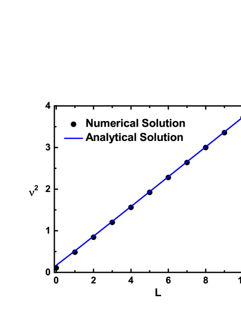
Figure 2: The analytical solution (solid line) (28) to the equation (25) compared to the numerical solution for the $L$-dependence of $\nu^{2}$.

Hence, Eqs. (16) through (18) are solved by (22) and (28). Putting them into (23) yields

$$M_{\bar{q}q}=w_{N}\nu_{N}+\frac{A_{N}}{\nu_{N}}+V_{0}$$ (30)

in which $\nu_{N}$ is given by (28) and

$$w_{N} =\frac{3}{2}+\frac{3ak_{\infty}}{N_{\nu}}+\frac{2a_{N}^{2}}{\nu^{4}\chi_{N}^{2}}$$ (31)

$$A_{N} =2\bar{m}^{2}\chi_{N}^{2}\left(\frac{\nu_{N}^{2}}{2a_{N}}\right)^{2}-\frac{ak_{\infty}}{1+a_{L}/\nu_{N}}$$ (32)

Since $\nu_{N}$ is solved from (16) through (18) in the relatively large-$N$ region, and the approximation (11) for the color Coulomb interaction applies better in the large distance regime, the prediction (30), obtained by the quark model (2) combined with AF method, should be more reliable for the high excited $\bar{q}q$ mesons. When $N$ is very large, $N_{\nu}$ as well as $\nu_{N}^{2}\rightarrow 2a\left(N+3/2\right)$, $\chi_{N}\rightarrow 1$ and $w_{N}\rightarrow 2$, which leads, by Eq. (30), to

$$M_{\bar{q}q}=2\nu_{N}+\left(2\bar{m}^{2}-ak_{\infty}\right)/\nu_{N}+V_{0}\,\text{,when }N\gg 1,$$ (33)

or

$$(M_{\bar{q}q}-V_{0})^{2}\propto 8aN,\text{when }N\gg 1,$$

This corresponds to the slope $(8a)^{-1}$ for the linear Regge trajectory on the $(N,(M_{\bar{q}q}-V_{0})^{2})$ plot that is predicted by the relativized quark model KangS:75 ; VeseliO:B96 . It is to be compared with the slope $1/(2\pi a)$ predicted by the relativistic string model Goto:71 ; Nambu:D74 .

We remark that when $N$ is large Regge linearity stems from the first and second term in (12), which appears to be of the harmonic-oscillator form: $a(N+3/2)+const$, as the most quark models with harmonic-oscillator-like confinement predicted. This changes, however, in our model due to the constraints (16)-(17) of the AF fields. The solutions (21) and (22) indicate $\mu=\mu_{m}/4\sim\sqrt{N}$ and $\nu\sim\sqrt{N}$ (namely,$\sqrt{\mu\nu}\sim\sqrt{N}$) in the large $N$ limit. Thus, when $N$ is large the first and second terms in (12) scale as $2\sqrt{2a_{N}}\sim\sqrt{N}$, hence the linear Regge behavior: $E_{N}^{2}\propto N$.

The mass relation (30) is inadequate in the low-$N$ region for two reasons rigorously. The first is obviously that Eqs. (28), (21) and (22) are not valid in the low-$N$ region, as seen in Table II (a,b), and that the approximation (11) does not apply in the low-lying states, as roughly shown in Table II (a,b). The second, more serious, is that the short distance behavior of the interquark interaction is far from established Bali01 ; KawanaiS:12 , e.g., the running of strong coupling remains unclear BrodskyT:B04 ; AguilarMN:A04 ; ShirkovSol:97 ; Ganbold:D10 . Thus, to find the mass relation for the low-$N$ region, we resort to the approximate linearity of the Regge trajectories that is established experimentally in meson spectrums AnisovichAS:PRD00 to constraint the prediction (30). By squaring (30), it follows that

$$\left(M_{\bar{q}q}-V_{0}\right)^{2} =2aw_{N}^{2}\left[N+\frac{3}{2}-\frac{\bar{m}^{2}}{a}\left(1-\frac{4e_{N}}{3}\right)\right.$$

$$+\left.\frac{k_{\infty}}{2}\left(h-2+\frac{4a_{L}}{\sqrt{2a_{N}}}\right)+D_{N}\right],$$ (34)

where

$$D_{N}=\frac{A_{N}}{aw_{N}}+\frac{a}{2\nu_{N}^{2}}\left(\frac{A_{N}}{aw_{N}}\right)^{2}.$$ (35)

The $N$-dependence of $\left(M_{\bar{q}q}-V_{0}\right)^{2}$ in (34) is nonlinear formally when compared to the Chew-Frautschi plot ChewF:61 . The constraining of (30) and extrapolating it to the relatively low-$N$ region can be done by making (34) quasi-linear in $N$. We note firstly that (34) is comparable to the linear Regge trajectories (1), provided that the $V_{0}$ is small when compared to the meson scale, $V_{0}/M_{\bar{q}q}\ll 1$. If we rewrite (34) in the form

$$\alpha_{N}^{\prime}\left(M_{\bar{q}q}-V_{0}\right)^{2}=N-\alpha_{N}(0),$$ (36)

in which the trajectory parameters $\alpha_{N}^{\prime}$ and $\alpha_{N}(0)$ are,

$$\frac{1}{\alpha_{N}^{\prime}}=2aw_{N}^{2}=\frac{9a}{2}\left[1+\frac{\left(2a_{N}/\nu_{N}^{2}\right)^{2}}{3\chi_{N}^{2}}+\frac{2ak_{\infty}}{N_{\nu}}\right]^{2},$$ (37)

$$-\alpha_{N}(0)=\frac{3}{2}-\frac{\bar{m}^{2}}{a}\left(1-\frac{4e_{N}}{3}\right)+\frac{k_{\infty}}{2}\left(h-2+\frac{4a_{L}}{\sqrt{2a_{N}}}\right)+D_{N},$$ (38)

respectively, then one can quasi-linearize (34) by expanding (37) and (38) on $1/N$. To order of $1/N$, the last term $D_{N}$ in (38) becomes

$$D_{N} \simeq\frac{\bar{m}^{2}}{a}\left(1-\frac{9\bar{m}^{2}}{4a_{N}}\right)+\frac{k_{\infty}}{2}\left(\frac{a_{L}}{\sqrt{2a_{N}}}-1\right)$$ (39)

$$+\frac{k_{\infty}}{16a_{N}}\left(ak_{\infty}(7-2h)-4a_{L}^{2}+4\bar{m}^{2}(5h-3)\right),$$ (40)

which leads to, when putting to (38),

$$-\alpha_{N}(0)=\frac{3}{2}+\frac{k_{\infty}}{2}\left(h-3+\frac{5a_{L}}{\sqrt{2a_{N}}}\right)+\frac{k_{\infty}\bar{m}^{2}}{4a_{N}}(5h-3).$$ (41)

The similar relation for the inverse slope (37) is

$$\frac{1}{\alpha_{N}^{\prime}}=8a\left[1+\frac{1}{2}\frac{3k_{\infty}}{2N+3}\left(1-\frac{h}{3}-\frac{2a_{L}}{\sqrt{2a_{N}}}\right)+\frac{\bar{m}^{2}}{2a_{N}}\right]^{2}.$$ (42)

When $N$ is very large Eq. (42) tends to a inverse slope: $\lim_{N\rightarrow\infty}$($\alpha_{N}^{\prime-1})=8a$, in consistent with claims in Refs. KangS:75 ; VeseliO:B96 .

One sees from (41) and (42) that the slope depends upon the dimensional parameters $a$ and upon the dimensionless parameters $k_{\infty}$, $\sqrt{a}/\Lambda$ and $\bar{m}^{2}/a$ weakly (suppressed by $N$ or $\sqrt{N}$) while the intercept depends upon $k_{\infty}\,$ strongly and also upon $\sqrt{a}/\Lambda$ and $\bar{m}^{2}/a$ weakly. Given (41) and (42), one rewrite (36) in the front of analytical mass formula for light mesons,

$$M_{q\bar{q}}=\left(1+K_{N}\right)\sqrt{8a\left[N-\alpha_{N}(0)\right]}+V_{0},$$ (43)

where

$$K_{N}=\frac{3ak_{\infty}}{4a_{N}}\left(1-\frac{h}{3}-\frac{2\lambda\sqrt{a}}{\Lambda\sqrt{2N+3}}\right)+\frac{m_{1}^{2}+m_{2}^{2}}{2a(2N+3)},$$ (44)

$$-\alpha_{N}(0)=\frac{3}{2}+\frac{k_{\infty}}{2}\left(h-3+\frac{5\lambda\sqrt{a}}{\Lambda\sqrt{2N+3}}\right)+\frac{k_{\infty}\bar{m}^{2}}{2a}\frac{5h-3}{2N+3}.$$ (45)

The formula (43) is the main result in this work. We see that the flavor dependence enters explicitly through the mass term $(m_{1}^{2}+m_{2}^{2})/a$. The following remarks are in order:

(i) The Hamiltonian (2), $H=\mu_{1}+\mu_{2}+V$, becomes almost independent of the quark masses in the light-light limit $m_{1,2}\rightarrow 0$ for which $\mu_{i}=\sqrt{|\mathbf{p}|^{2}+m_{i}^{2}}\rightarrow|\mathbf{p}|$. The same it true when $L$ is large since $|\mathbf{p}|^{2}$ has the expectation $\sim N$ in the harmonic basis $|nL\rangle$. See (21) and (22). The $m_{1,2}$-dependence of the system mass is thereby suppressed by $N$. This accounts for the asymptotic flavor independence happened in Table II(b) that $\mu_{1,2}$ tend to be same with $L$ increases.

(ii) In spite of assumption $a_{N}\propto N\gg 1$ in obtaining (43) and (30) from the Hamiltonian (2), the quasi-linearizing of the model prediction (34) makes it applicable in the low-excited states, thanks to the Regge phenomenology for light mesons.

(iii) The mass formula (43) goes beyond the native prediction of the relativized quark model in that it employs merely the large-$N$ asymptotic behaviors of the model spectrum that is implied in relativistic quark model.

(iv) The ultra-relativistic contributions from QCD string rotating to the orbital angular momentum and to the energy of meson has not taken into account in (43), which can otherwise enhance the confining parameter $a$ by a factor of $8a/(2\pi a)=4/\pi$ in the high excited states of mesons, which will be discussed in the section 4 and section 5.

IV Numerical results and discussions

In this section, we confront the mass formula (43) with the experiments and other approaches. As explained in the text, we are of mainly interest in the orbitally excited states, where our approximation is expected to work best. For this, we choose six families of light mesons, marked by $\pi/b$, $\rho/a$, $\eta/h$, $\omega/f$, $K^{\ast}$ and $\phi/f^{\prime}$. The members we pick for the trajectories are always the lightest known states with appropriate quantum numbers. In each family, the quantum numbers of $P$ and $C$ alternate their values across the trajectory provided that they are mainly made of $\bar{q}q$ system with the parity $P=(-)^{L+1}$ and $C=(-)^{L+S}$. Furthermore, the $J=0$ state in the $\pi/b$-trajectory, which is actually the pion, has been excluded due to its abnormally low mass.

In Table III, the selected family members are shown explicitly, together with the linear fit for the observed mass squared $M^{2}$ v.s. $L$, with the data taken entirely from the Particle Data Group’s (PDG) 2016 Review of Particle Physics Patrignani:C16 . We also list the corresponding slope $\alpha^{\prime}$, intercept and the MS error for linear fit defined by $\chi_{MS}^{2}=\sum_{L}(M_{L}^{Th}-M_{L}^{Exp})^{2}/L_{\max}$ where the index $L$ runs from $0$ ($1$ for the $\pi/b$ trajectory) to the maximal value $L_{\max}$ of the orbital angular momentum. From the linear fit shown in Table III one sees that the linear relation (1) applies for the trajectories of $\rho/a$ and $\omega/f$ for which intercept is about $-0.5$, but is violated for the $\pi/b$, $\eta/h$ and $\phi/f^{\prime}$ trajectories for which the intercepts are about $-0.3$,$-0.1$ and $-0.74$, respectively. The $K^{\ast}$ trajectory can fit the relation (1) very roughly.

We use the mass formula (43), with $K_{N}$ and $-\alpha_{N}(0)$ given by (44) and (45), to map the observed masses in each family in Table III, guided globally by corresponding linear fit in the Table III. For the family of $\eta/h$, with the ideal mixing $\Phi(\eta/h)=\left(\sqrt{2}nn-2\bar{s}s\right)/\sqrt{6}$ assumed for the flavor content, we use the mass formula

$$M_{\eta/h}=\frac{1}{3}M_{n\bar{n}}+\frac{2}{3}M_{s\bar{s}},$$ (46)

with the masses $M_{n\bar{n}}$ and $M_{s\bar{s}}$ given by (43) and $2\bar{m}^{2}$($=m_{1}^{2}+m_{2}^{2}$)$=2m_{ud}^{2}$ and $2m_{s}^{2}$, respectively. The results for the optimal parameters ($a,\Lambda$,$V_{0}$) determined are shown in Table IV. Due to its abnormal nature, we always take the family of $\eta/h$ to be abnormal in this work.

As can seen in the Table IV, the values of $V_{0}$ are all negative, as argued in Gromes:Z81 for the non-relativistic limit of the Bethe-Salpeter equation. Furthermore, apart from the family of $\eta/h$ the model parameters ($a,\Lambda$) are taken values around

$$\begin{array}[c]{r}a=0.147\pm 0.005\text{GeV}^{2}\text{,}\\ \Lambda=0.184\pm 0.072\text{GeV.}\end{array}$$ (47)

The small fluctuation implies, especially for $a$, that $a$ and $\Lambda$ keep the same approximately. In contrast, the linear fit in Table III (the last column) implies an averaged string tension (assuming the QCD string picture)

$$a\text{(Linear fit)}=0.189\pm 0.0135\text{GeV}^{2}\text{,}$$ (48)

with much larger fluctuation than that in (47). We note that in the above analysis $\eta/h$ trajectory is excluded as an exceptional case. In this sense, the confining parameter $a$ is almost universal. A detailed comparison of the result (47) with other predictions in the literatures is shown in Table V.

One can observe from Table V that the values of $a$ is close to that predicted by Veseli and Olsson VeseliO:B96 and the linearly confining parameter for the heavy-quarkonia in lattice QCD KawanaiS:12 , whereas it is smaller, about $20\%$, than that in the other quark models cited. In the end of Section 4 and in the Section 5, we address this issue in details.

We list the mass predictions by the formula (43) and the experimentally observed masses in Table VI. As seen there, an good agreement is achieved between the mass predictions and the observed data for all families, if considering the spin-dependent interaction is ignored in present work. In spite of deviations about $8\%$ for some states the mass formula (43) is confirmed qualitatively at the level of the average deviation less than $5\%\,$. The best agreement occurs for the $\omega/f$ trajectory for which the average mass deviation is about $3\allowbreak 0$MeV.

In Table VII, we list the slopes given by the formula (42), other calculations and the analysis of the experimental data cited.

To answer why the determined value of the confining parameter $a$ in (47) is relatively smaller than that in the other quark models cited in Table V, we would like emphasize that our method to solve the model differs from that in the most quark models in that it requires the light quark mass to be quite small (close to the bare mass). As stated in the introduction, our mass formula is obtained not only by applying the AF method to solve the model (2) in the relatively large-$N$ case, but also using the empirical Regge linearity that is confirmed experimentally in the large-$N$ states. The later purpose is fulfilled by quasi-linearizing the quark model formula for the mass squared around the high excited states. When mapping the observed masses, the parameters in our model, guided also by the linear fit in Table III, are mainly fixed so that the behavior of the high excited states is highlighted, where $M_{q\bar{q}}^{2}\simeq 8aL$.

In the most of relativistic quark models cited, however, the parameter setup crucially relies on the low-lying spectrum in which the quark masses are heavy, roughly around $200\sim 300$MeV. This setup of the quark mass will violate the linearity of Regge trajectories of the low-lying states, provided that no further relativistic treatment similar to that in GodfreyIsgur:85 is made to the potential $V$ in (3) correspondingly. This can be shown using the semiclassical approximation in the Section 5.

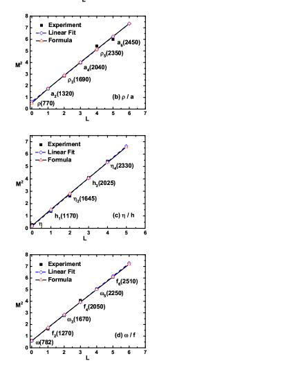
Figure 3: The mass squared $M^{2}$ vs. orbital angular momentum $L$ for the nonstrange mesons. Four trajectories are the $\pi/b$ family (a), the $\rho/a$ family (b), the $\eta/h$ family (c) and the $\omega/f$ family (d).

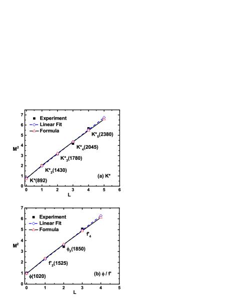
Figure 4: The mass squared $M^{2}$ vs. orbital angular momentum $L$ for the strange mesons. Two trajectories are the $K^{\ast}$ family (a) and the $\phi/f^{\prime}$ family (b).

One sees that our Regge-like mass relation (43) for the orbitally-excited light mesons agrees well with the observed mass spectrum. Moreover, the relation has a feature that supports a universality underlying in formation dynamics of the light meson in the following sense:

(i) The quark mass dependence of the light meson spectroscopy is suppressed doubly by $\bar{m}^{2}$ and ${1/N}$ in the high excited states.

(ii) The confining parameter $a$ and the cutoff $\Lambda$ is nearly same for all families of the mesons considered, except for the $\eta/h$ trajectory.

We remark that Table IV does not indicate flavor-independence of $V_{0}$ though their dependence on the flavor contents is weak. This is so because $V_{0}$ in practice accounts for all residual contributions including the averaged spin-dependent interaction which depends spin nature of mesons eventually in net value.

Accepting the above, one infers that the members of the $\eta/h$ trajectory should contain exotic components which makes them exceptional, as seen in Table IV. The usual mixing $(\sqrt{2}nn-2\bar{s}s)/\sqrt{6}$ for $\eta/h$ trajectory is not adequate for accounting for their abnormal feature.

V Semiclassical approximation

Before arguing why the quark mass $m_{i}$ should be small in our model, let us check numerically what value the confining parameter will be equivalent to when the relativistic correction due to the rotating of QCD string tied to quarks is taken account into. In the quark model, this correction has been ignored intrinsically by the potential assumption of the interquark interaction. Nevertheless, one can check how the data mapping of model makes up the deficit by comparing the slopes between them. Our model predicts the slope $1/(8a)$ in the high excited limit of (42), while the rotating string model predicts the Regge slope $1/(2\pi\sigma)$, where $\sigma$ is the string tension. The result $a=0.147$ in (47) is equivalent, under the following correspondence,

$$\frac{1}{8a}\longleftrightarrow\frac{1}{2\pi\sigma},$$ (49)

to the string tension $\sigma=0.187$GeV², which agrees well with that in the most of relativistic quark models.

While it has been already known in the past Dias:Z85-86 ; CeaNP:D82 ; CeaNP:D83 ; Goebel:D90 ; VeseliO:B96 we would like to reemphasize the connection between the linear confinement, linear trajectories and relativistic dynamics LuchaSG:RP91 , which is helpful to understand the results in Table II (a,b), Table V and VI. Firstly, we note that the leading Regge slope follows from the correspondence (classical) limit. Let us consider the radially-lowest state of (2) but with a given large $L$ which corresponds to the circular orbital motion of quark at large $r$ and large $p$. The minimal energy condition $(\partial H/\partial r)|_{L}\equiv 0$ for $H$ in (2) implies that $L|\mathbf{p}|[\mu_{1}^{-1}+\mu_{2}^{-1}]=ar^{2}$, with $\mu_{i}=\sqrt{|\mathbf{p}|^{2}+m_{i}^{2}}$. If one takes $m_{1,2}\rightarrow 0$ (the light-light limit), then $\mu_{1,2}\rightarrow|\mathbf{p}|$ and $|\mathbf{p}|^{2}\rightarrow L^{2}/r^{2}$($p_{r}\ll 1$ ).   It follows that

$$H\rightarrow 2|\mathbf{p}|+ar\text{, }2L=ar^{2},$$ (50)

which yields (when using $|\mathbf{p}|=L/r$ and eliminating $r$)

$$\alpha_{LL}^{\prime}\text{(}L\gg 1\text{)}=\frac{L}{H^{2}}=\frac{1}{8a},$$ (51)

This is in consistent with (42).

It is of heuristic to ”derive” the Regge relation (51) with the help of Bohr-like argument for Hydrogen atom. From (50) one has, for the large-$L$ state $|0L\rangle$,

$$\langle H\rangle_{L}=2a\langle r\rangle_{L},2L=a\langle r^{2}\rangle_{L},$$ (52)

with $n=0$ assumed. Usage of (27) yields $\langle r\rangle_{L}=\nu_{N}/a=\sqrt{2L/a}$. It follows that

$$\langle H\rangle_{L}=\sqrt{8aL},\langle r^{2}\rangle_{L}\sim\frac{L}{a},$$ (53)

as required to have (51).

On the other hand, if we assume $m_{1,2}/M$ is not small, with $M$ the mass of the quark-antiquark system, a similar analysis that leads to (14) yields (in the case that $m_{1,2}=m$, $L=0$) a WKB quantization condition

$$(n+b^{\prime})\pi=\int_{-(M_{c}-m)/a}^{(M_{c}-m)/a}dx\sqrt{(M_{c}-a|x|)^{2}-m^{2}}.$$

with $M_{c}=M/2$. It follows that

$$2a\pi(n+2b^{\prime})=M^{2}F_{d}\left(\frac{2m}{M}\right),$$ (54)

$$F_{d}(\tau)=\sqrt{1-\tau^{2}}-\tau^{2}\ln\left(\frac{1+\sqrt{1-\tau^{2}}}{\tau}\right)$$ (55)

where the procedure $n\rightarrow n/2$ was used to remove the reflection ($x\rightarrow-x$) degeneration (double counting of the radial space of quark motion). One sees from FIG. 5 that the deviation from the linear Regge trajectory, given by $1-F_{d}(2m/M)$, can be up to $\allowbreak 25\%$ for $m=220$MeV and $\allowbreak 40\%$ for $m=300$MeV if choosing $M$ to be mass of $a_{2}(1318)$ $2^{++}$. This explains why the quark mass $m_{i}$ should be small in our model, compared to the most of the quark models cited in Table V.

Figure 5: $F_{d}$ as a function of $2m/M$.

It is of interest to note that the method in Section 2 and 3 can be extended to the case of heavy-light mesons which consist of a heavy quark and a light antiquark, though this is not the main issue in this work. Starting again from the Hamiltonian (2), with $m_{1}=m_{Q}$ being the heavy quark mass and $m_{2}=m_{q}$ the mass of light antiquark, and assuming $m_{Q}$ to be heavy, one has, for the Hamiltonian of heavy-light mesons,

$$H^{hl} =m_{Q}+\frac{\mathbf{p}^{2}}{2m_{Q}}+\sqrt{\mathbf{p}^{2}+m_{q}^{2}}+ar$$

$$=m_{Q}+\frac{\mathbf{p}^{2}}{2m_{Q}}+\min_{\mu_{2}}\left\{\frac{\mathbf{p}^{2}+m_{q}^{2}}{2\mu_{2}}+\frac{\mu_{2}}{2}\right\}$$

$$+\min_{\nu}\left\{\frac{a^{2}r^{2}}{2\nu}+\frac{\nu}{2}\right\},$$ (56)

where the color-Coulomb term and $V_{0}$ are ignored for simplicity. Transforming to the center-of-mass system, one has

$$H^{hl}-m_{Q}=\frac{\mathbf{p}^{2}}{2\mu}+\frac{\mu}{2}\left(\frac{a^{2}}{\mu\nu}\right)r^{2}+\frac{\mu_{2}+\nu}{2}+\frac{m_{q}^{2}}{2\mu_{2}},$$ (57)

with $\mu=\mu_{2}/(1+\mu_{2}/m_{Q})$ the reduced mass of the quarks. The similar analysis as in section 2 yields

$$E_{N}(\mu_{2},\nu)=\frac{a_{N}}{\sqrt{\mu\nu}}+\frac{\mu_{2}+\nu}{2}+\frac{m_{q}^{2}}{2\mu_{2}}.$$ (58)

The minimization of (58) with respect to $\mu_{2}$ and $\nu$ gives $\mu_{2}=b_{N}^{1/3}[1-\frac{1}{3}b_{N}^{1/3}/m_{Q}]$ and $a_{N}^{2}=b_{N}^{1/3}\left[1-\frac{4}{3}b_{N}^{1/3}/m_{Q}\right]$ with $b_{N}\equiv a_{N}^{2}/\nu$. Assuming $m_{Q}\gg 1$, one can show

$$\nu^{2} =a_{N}=(a_{N}\nu)^{2/3}=\mu\nu,$$

$$\mu_{2} =b_{N}^{1/3}=\nu,$$

which enables us to rewrite (58) as

$$E_{N}-m_{Q}=2\sqrt{a\left(N+\frac{3}{2}\right)}+\frac{m_{q}^{2}}{2\sqrt{a_{N}}},$$ (59)

or equivalently, as the linear Regge relation $(E_{N}-m_{Q})^{2}=4a\left(N+3/2\right)$ in the heavy-light limit. The later relation has an inverse slope $4a$, being a half of that of the light-meson trajectories at light-light limit: $\alpha_{HL}^{{}^{\prime}}=2\alpha_{LL}^{{}^{\prime}}$. This feature has been pointed out in Refs. JohnsonN:PRD79 ; VeseliO:B96 ; Olsson:D1997 ; Selem:06 . Comparing with the case of the light mesons, the above argument using the AF method differs in that only one auxiliary field ($\mu_{2}$) is introduced for the kinematic of light quark, with the heavy quark treated nonrelativistically. This is in consistent with the observation Olsson:D1997 that linear Regge trajectories result from light quark kinematics and linear confinement.

VI Summary and concluding remarks

Up to date, mesons remain to be the ideal subjects for the study of strong interactions in the strongly coupled regime. Even though we have a theory of the strong interactions (QCD), we still know very few about the physical states of the theory which are crucial to understand QCD eventually. To a large extent our knowledge of hadron physics relies on phenomenological models, for instance, the quark models and others. Though successful, the quark models manifest themselves in various forms, and their predictions can differ appreciably GodfreyN:P1999 , in particular, for the excited states. So it entails constraining of the model predictions by experiment in the case of the excited states.

For the excited mesons, which can be generated abundantly, the issues such as whether non-conventional states (exotics) emerge becomes of great interest in the light sector of hadrons. However, to have hope of distinguishing between conventional and exotic mesons, it is crucial for us to understand conventional meson spectroscopy well GodfreyN:P1999 ; AmslerT:RP04 . Great efforts have been made to describe light meson spectrum RujulaGG:D75 ; KangS:D75 ; BasdevantB:C85 ; GodfreyIsgur:85 ; EbertFG:D09 in an universal way, in which model parameters are assumed to be more or less universal. These descriptions succeeded remarkably in describing the most observed states. Meanwhile, question as to whether the universality persists remains to be of important when new discovered states are considered.

In this work, we addressed the orbitally-excited Regge spectrum of the light mesons and their universality using relativized quark model combined with approximated linearity of Regge trajectory. By solving the model with the auxiliary field method and quasi-linearizing the solution near the asymptotic limit of the large orbital angular momentum, an new Regge-like mass relation is proposed for the orbitally excited mesons which supports the universality that the quark mass dependence of the light meson spectroscopy is suppressed significantly and the confining parameters $a$ is almost same for all families except for $\eta/h$-trajectory. The resulted predictions are found to be in good agreement with the observed data of light mesons.

An explicit expressions for the Regge slope and intercept are obtained and one mass of the high exciton is predicted for each family in Table VI. We suggest that the members of the $\eta/h$ trajectory may contain components of exotic.

We have also discussed our results in comparison with the results from the string (flux-tube) picture of mesons Nambu:D74 ; Goto:71 and from the other quark models. By the way, we presented a semiclassical argument that the inverse slopes on the radial and angular-momentum Regge trajectories are equal in the massless limit of quarks, being in consistent with the suggestions in the literatures.

APPENDIX A

In order to solve (25) using the method of homotopic analysis (HA) Liao , we rewrite two nonlinear equations (26) with $\bar{m}^{2}=0$ and (25) in the form of $L_{\nu}(q)=0$ and $NL_{\nu}(q)=0$, where

$$L_{\nu}(q) \equiv\frac{3}{2}-\frac{6a_{N}^{2}}{\nu^{4}},$$ (A-1)

$$NL_{\nu}(q) =\frac{3}{2}+\frac{3ak_{\infty}q^{2}}{N_{\nu}}-\frac{6a_{N}^{2}}{\nu^{4}\chi_{N}^{2}}-\frac{4ak_{\infty}\nu q^{2}}{N_{\nu}^{3/2}}+\frac{16ak_{\infty}a_{N}^{2}q^{2}}{\nu^{3}\chi_{N}^{3}N_{\nu}^{3/2}}$$

$$+\frac{q^{2}\bar{m}^{2}}{2a_{N}^{2}}\left(3\nu^{2}\chi_{N}^{2}q^{-2}-8ak_{\infty}\frac{\nu^{3}\chi_{N}}{N_{\nu}^{3/2}}\right)$$ (A-2)

are two functionals for defining the two equations (26) and (25). The sole difference is that a new and real artificial parameter $q$ $(0\leq q\leq 1)$ is introduced in the above two equations to indicate the order of smallness (when $N$ becomes large) by following scaling rules (based on $\nu^{2}\propto N\propto q^{-2}$)

$$\nu \rightarrow\nu/q\propto\sqrt{N},a_{N}\rightarrow a_{N}/q^{2}$$

$$N_{\nu} \rightarrow N_{q}/q^{2},N_{q}\equiv(\nu+qa_{L})^{2},$$

$$\chi_{N} \rightarrow\chi_{q}\equiv 1+2ak_{\infty}/N_{q}.$$ (A-3)

The idea of the homotopic analysis (HA) Liao is to solve the functional equation $G(L_{\nu}(q),NL_{\nu}(q),q)$ $=0$ with

$$G(L_{\nu}(q),NL_{\nu}(q),q)\equiv(1-q)L_{\nu}(q)-hqNL_{\nu}(q),$$ (A-4a)

or equivalently,

$$(1-q)L_{\nu}(q)=hqNL_{\nu}(q),$$ (A-4b)

before solving the nonlinear equation $NL_{\nu}(q=1)=0$ which is (25). Here, $h$ is the accelerating factor Liao remained to be fixed either by the platform in the plot window for the characteristic quantity in the model or comparing with the numerical solution. When $q=0$, $G(L_{\nu}(q),NL_{\nu}(q),q)=0$ becomes (A-1) while it becomes (25) when $q=1$. If one solves (A-4b) (helpful if using the computer) up to the third order of $q$, one finds

$$\nu^{2} =2a_{N}-2ak_{\infty}q^{2}+ak_{\infty}\left(h+\frac{4a_{L}}{\sqrt{2a_{N}}}\right)q^{3}$$

$$-2\bar{m}^{2}\left(1+\frac{ak_{\infty}}{2a_{N}}(3+4h)q^{2}\right),$$ (A-5)

which gives (28) when putting $q=1$.

References

- (1) C. Patrignani et al. [Particle Data Group], The Review of Particle Physics, Chin. Phys. C 40, 100001 (2016).
- (2) J. D. Weinstein and N. Isgur, Phys. Rev. Lett. 48, 659 (1982).
- (3) J. D. Weinstein and N. Isgur, Phys. Rev. D 27, 588 (1983).
- (4) S. Godfrey and J. Napolitano, Rev. Mod. Phys. 71, 1411 (1999).
- (5) C. Amsler and N. A. Tőrnqvist, Phys. Rept. 389, 61 (2004).
- (6) G. F. Chew and S. C. Frautschi, Phys. Rev. Lett. 7, 394 (1961).
- (7) A. V. Anisovich, V. V. Anisovich and A. V. Sarantsev, Phys. Rev. D 62, 051502 (2000).
- (8) P. Masjuan, E. R. Arriola and W. Broniowski, Phys. Rev. D 85, 094006 (2012).
- (9) A. De Rujula, H. Georgi and S. L. Glashow, Phys. Rev. D 12, 147 (1975).
- (10) J. S. Kang and H. J. Schnitzer, Phys. Rev. D 12, 841 (1975).
- (11) J. L. Basdevant and S. Boukraa, Z. Phys. C 28, 413 (1985).
- (12) S. Godfrey and N. Isgur, Phys. Rev. D 32, 189 (1985).
- (13) D. Ebert, R. N. Faustov and V. O. Galkin, Phys. Rev. D 79, 114029 (2009).
- (14) M. G. Olsson, Phys. Rev. D 55, 5479 (1997).
- (15) G. S. Sharov, String Models, Stability and Regge Trajectories for Hadron States, arXiv:1305.3985 [hep-ph].
- (16) J. Sonnenschein and D. Weissman, JHEP 1408, 013 (2014).
- (17) M. M. Brisudova, L. Burakovsky and J. T. Goldman, Phys. Rev. D 61, 054013 (2000).
- (18) K. Johnson and C. Nohl, Phys. Rev. D 19, 291 (1979).
- (19) S. S. Afonin, Phys. Lett. B 576, 122 (2003).
- (20) P. D. B. Collins, An Introduction to Regge Theory and High-Energy Physics (Cambridge Univ. Press, Cambridge, 1977).
- (21) Y. Nambu, Phys. Rev. D 10, 4262 (1974).
- (22) T. Goto, Prog. Theor. Phys. 46, 1560 (1971).
- (23) S. S. Afonin, Phys. Lett. B 639, 258 (2006).
- (24) S. S. Afonin, Mod. Phys. Lett. A 22, 1359 (2007).
- (25) P. Bicudo, Phys. Rev. D 76, 094005 (2007).
- (26) H. Forkel, M. Beyer and T. Frederico, Int. J. Mod. Phys. E 16, 2794 (2007).
- (27) H. Forkel, M. Beyer and T. Frederico, JHEP 0707, 077 (2007).
- (28) J. S. Kang and H. J. Schnitzer, Phys. Rev. D 12, 841 (1975).
- (29) K. M. Maung, D. E. Kahana and J. W. Norbury, Phys. Rev. D 47, 1182 (1993).
- (30) S. Veseli and M. G. Olsson, Phys. Lett. B 383, 109 (1996).
- (31) B. Silvestre-Brac, C. Semay and F. Buisseret, J. Phys. A: Math. Theor. 41, 425301 (2008).
- (32) B. Durand and L. Durand, Phys. Rev. D 25, 2312 (1982).
- (33) D. B. Lichtenberg, W. Namgung, E. Predazzi and J. G. Wills, Phys. Rev. Lett. 48, 1653 (1982).
- (34) B. Durand and L. Durand, Phys. Rev. D 30, 1904 (1984).
- (35) S. Jacobs, M. G. Olsson and C. Suchyta III, Phys. Rev. D 33, 3338 (1986).
- (36) W. Lucha, H. Rupprecht and F. F. Schöberl, Phys. Rev. D 46, 1088 (1992).
- (37) G. S. Bali, Phys. Rept. 343, 1 (2001).
- (38) T. Kawanai and S. Sasaki, Prog. Part. Nucl. Phys. 67, 130 (2012).
- (39) S. Chekanov et al. [ZEUS Collaboration], Phys. Lett. B 560, 7 (2003).
- (40) S. Bethke, J. Phys. G 26, R27 (2000).
- (41) D. V. Shirkov and I. L. Solovtsov, Phys. Rev. Lett. 79, 1209 (1997).
- (42) G. Ganbold, Phys. Rev. D 81, 094008 (2010).
- (43) M. Bruno et al. [ALPHA Collaboration], Phys. Rev. Lett. 119, 102001 (2017).
- (44) S. J. Brodsky and G. F. de Teramond, Phys. Lett. B 582, 211 (2004).
- (45) A. C. Aguilar, A. Mihara and A. A. Natale, Int. J. Mod. Phys. A 19, 249 (2004).
- (46) Duojie JIA, C. Q. Pang and A. Hosaka, Int. J. Mod. Phys. A 32, 1750153 (2017).
- (47) C. Semay, B. Silvestre-Brac and I. M. Narodetskii, Phys. Rev. D 69, 014003 (2004).
- (48) A. M. Polyakov, Gauge Fields and Strings (Harwood Academic Publishers, Poststrasse, 1987).
- (49) E. L. Gubankova and A. Yu. Dubin, Phys. Lett. B 334, 180 (1994).
- (50) V. L. Morgunov, A. V. Nefediev and Yu. A. Simonov, Phys. Lett. B 459, 653 (1999).
- (51) Yu. S. Kalashnikova and A. V. Nefediev, Phys. Lett. B 492, 91 (2000).
- (52) J. P. Elliott, Proc. Roy. Soc. Lond. A 245, 128 (1958).
- (53) L. I. Schiff, Quantum Mechanics (McGraw-Hill Book Company, New York, 1968).
- (54) S. J. Liao, Appl. Math. Comput. 147, 499 (2004).
- (55) D. Gromes, Z. Phys. C 11, 147 (1981).
- (56) L. P. Fulcher, Z. Chen and K. C. Yeong, Phys. Rev. D 47, 4122 (1993).
- (57) D. S. Hwang and G. H. Kim, Phys. Rev. D 53, 3659 (1996).
- (58) J. L. Basdevant and S. Boukraa, Z. Phys. C 28, 413 (1985).
- (59) P. Cea, P. Colangelo, G. Nardulli, G. Paiano and G. Preparata, Phys. Rev. D 26, 1157 (1982).
- (60) P. Cea, G. Nardulli and G. Paiano, Phys. Rev. D 28, 2291 (1983).
- (61) C. Goebel, D. LaCourse and M. G. Olsson, Phys. Rev. D 41, 2917 (1990).
- (62) W. Lucha, F. F. Schöberl and D. Gromes, Phys. Rept. 200, 127 (1991).
- (63) A. Selem and F. Wilczek, Hadron systematics and emergent diquarks, arXiv:hep-ph/0602128.