Gravitational Interactions of Finite Thickness Global Topological Defects with Black Holes

Abstract

It is well known that global topological defects induce a repulsive gravitational potential for test particles. ’What is the gravitational potential induced by black holes with a cosmological constant (Schwarzschild-de Sitter (S-dS) metric) on finite thickness global topological defects?’. This is the main question addressed in the present analysis. We also discuss the validity of Derrick’s theorem when scalar field configurations are embedded in non-trivial gravitational backgrounds. In the context of the above stated question, we consider three global defect configurations: a finite thickness spherical domain wall with a central S-dS black hole, a global string loop with a S-dS black hole in the center and a global monopole near a S-dS black hole. Using an analytical model, numerical simulations of the evolving spherical wall and energetic arguments we show that the spherical wall experiences a repelling gravitational potential due to the mass of the central black hole. This potential is further amplified by the presence of a cosmological constant. For initial domain wall radius larger than a critical value, the repulsive potential dominates over the wall tension and the wall expands towards the cosmological horizon of the S-dS metric where it develops ghost instabilities (the kinetic term changes sign). For smaller initial radius, tension dominates and the wall contracts towards the black hole horizon where it also develops ghost instabilities. We also show, using the same analytical model and energetic arguments that a global monopole is gravitationally attracted by a black hole while a cosmological constant induces a repulsive gravitational potential as in the case of test particles. Finally we show that a global string loop with finite thickness experiences gravitational repulsion due to the cosmological constant which dominates over its tension for a radius larger than a critical radius leading to an expanding rather than contracting loop.

I Introduction

It is well known that a non-trivial background metric has a significant effect of the dynamical equations determining the evolution of scalar fields. For example a non-trivial spherically symmetric background metric of the form

$$ds^{2}=f(r)dt^{2}-f(r)^{-1}dr^{2}-r^{2}(d\theta^{2}+\sin^{2}\theta d\phi^{2})$$ (1)

leads to a modified Klein-Gordon equation of the form

$$\biggl{[}-\frac{r^{2}}{f(r)}\frac{\partial^{2}}{\partial t^{2}}+\frac{\partial}{\partial r}\biggl{(}r^{2}f(r)\frac{\partial}{\partial r}\biggr{)}-\mathbf{L}^{2}-m^{2}r^{2}\biggr{]}\Phi=0\ ,$$ (2)

where $\mathbf{L}$ is the angular momentum operator in spherical coordinates. Eq. (2), its generalization for axisymmetric backgrounds and the corresponding Dirac equation have been well studied Rowan and Stephenson (1976, 1977); Page (1976); Mukhopadhyay and Chakrabarti (1999); Elizalde (1987, 1988); Bezerra et al. (2014); Vieira and Bezerra (2016); Sakalli (2016); Vieira et al. (2017); Kraniotis (2018); Bezerra et al. (2017); Kraniotis (2016), exact solutions have been found using separation of variables and physical implications have been investigated (normal modes, Hawking radiation etc).

In the presence of a nonlinear scalar field potential $V(\Phi)$ the corresponding generalized scalar field dynamical equations have been studied at a smaller extend and mainly in the context of the existence of stable static solutions. In a flat 3+1 dimensional background such solutions are not allowed by Derrick’s theoremDerrick (1964) which states that in 3+1 dimensions, any finite energy initially static scalar field configuration with canonical scalar kinetic terms and non-negative potential energy is unstable and energetically favoured to shrink and collapse. In a curved background this instability and lack of static solutions has been shown to persist in specific cases (eg charged rotating black holeRadmore and Stephenson (1978); Palmer (1979)) but no general statement has been made for arbitrary gravitational background. In the present analysis we demonstrate (among other results) that a proper choice of $f(r)$ in the background metric can lead to static and perhaps to metastable solutions thus evading the conclusion of Derrick’s theorem.

It has been shown that it is possible to evade Derrick’s theoremDerrick (1964); Perivolaropoulos (1992a) even in flat space and construct static topologically stable (or nontopological metastableHindmarsh (1993); Achucarro et al. (1992); James et al. (1993); Vachaspati (1992); James et al. (1992); Perivolaropoulos (1994); Achucarro and Vachaspati (2000)) scalar field solutions. Such approaches include the introduction of gauge fieldsNielsen and Olesen (1973); ’t Hooft (1974); Polyakov (1974); Perivolaropoulos (1993a, 2000, b, 2000), the consideration of stationary rather than static solutionsColeman (1985); Kusenko (1997); Axenides et al. (2000); Perivolaropoulos (1994); Copeland et al. (1995) and the violation of the finite energy assumption madeBazeia et al. (2007, 2003); Axenides et al. (2000); Perivolaropoulos (1992b) with the possible introduction of non-standard kinetic termsBabichev (2006) in 3+1 or in higher dimensionsOlasagasti and Vilenkin (2000); Gregory (2000). A scalar field configuration with diverging energy in 3+1 dimensions would require a large scale cutoff which is naturally present in many physical systems. For example in a cosmological setup the role of the cutoff can be played by the horizon while in a condensed matter system the cutoff scale would be the size of the system. Global topological defectsVilenkin (1985); Vilenkin and Shellard (2000); Brandenberger (1994); Hindmarsh and Kibble (1995); Sakellariadou (2007) in three spatial dimensions constitute such stable scalar field configurations with diverging energy and have observable effects in both condensed matter systemsMermin (1979); Chuang et al. (1991); Digal et al. (1999); Zurek (1996); Bowick et al. (1994) and in cosmologyDurrer et al. (2002); Pen et al. (1997); Vilenkin (1981a); Brandenberger (1994); Bazeia et al. (2005); Perivolaropoulos (2005); Sikivie (1982); Lukas et al. (1999); Harari and Sikivie (1987); Kusenko and Shaposhnikov (1998); Enqvist and McDonald (1998); Durrer et al. (1999); Pen et al. (1997); Bennett and Rhie (1990); Perivolaropoulos (1992c); Pogosian and Vachaspati (1999); Perivolaropoulos et al. (1990); Perivolaropoulos (1993c); Moessner et al. (1994). They include global monopoles Barriola and Vilenkin (1989); Harari and Lousto (1990); Hiscock (1990); Dando and Gregory (1998); Barros and Romero (1997) (spherical field configurations) global strings Harari and Sikivie (1988); Vilenkin (1981b); Cohen and Kaplan (1988) (axial field configurations) and domain walls Vilenkin (1981a); Sikivie (1982); Csaki et al. (2000); Gremm (2000a, b) (planar configurations).

Global defects constitute regions of physical space that may form during phase transitions in the Early Universe where vacuum energy of an early symmetric phase gets trapped for topological reasons. Unlike their gauged counterpartsHindmarsh and Kibble (1995), global defects can not be approximated as being infinitely thin since the scalar field approaches its vacuum expectation value as a power law rather than exponentially. Thus they generically have a core of finite thickness of the order of the symmetry breaking scale that gave rise to the defects. This core may in general have non-trivial field structure with interesting effects in cosmology and condensed matter systemsAxenides and Perivolaropoulos (1997); Axenides et al. (1998).

The evolution of topological defects and especially strings in curved backgrounds has been investigatedDe Villiers and Frolov (1998a, b); Lonsdale and Moss (1988); Dabrowski and Larsen (1997); Dubath et al. (2007); Page (1998); de Vega and Egusquiza (1994); Frolov et al. (1989); Natário et al. (2018); Christensen et al. (1998); Porfyriadis and Papadopoulos (1998); Larsen (1994) under the thin defect approximation where the defects are assumed to have zero thickness and thus propagate via simplified forms of the action. For example the action that describes the evolution of a zero thickness string is the Nambu-Goto action which is proportional to the area of the world-sheet of the string. This is a good approximation for gauged defects but it is not applicable for global defects where the finite thickness and the field structure can not usually be ignored. The evolution of global defects in non-trivial gravitational backgrounds requires the solution of the full dynamical field equations derived by variation of the scalar field action with the appropriate background metric. Such analyses and numerical simulations have been performed in the context of homogeneous expanding FRW background metrics for global defectsYe and Brandenberger (1990a); Press et al. (1989); Lopez-Eiguren et al. (2017a); Hagmann and Sikivie (1991) and gauged stringsYe and Brandenberger (1990b); Bevis et al. (2007a, b); Daverio et al. (2016); Lopez-Eiguren et al. (2017b); Hindmarsh et al. (2017); Urrestilla and Vilenkin (2008) but not (to our knowledge) in inhomogeneous, spherically symmetric or axisymmetric black hole metrics.

Thus, an intersting question that needs to be adressed is the following: ’Is there an attractive interaction between black holes and global defects?’. How does the answer change if a cosmological constant is also present?’. Previous studies invetigating the global defect metric, have indicated that due to their vacuum energy, global topological defects induce a repulsive gravitational potential on test particlesHarari and Sikivie (1988); Harari and Lousto (1990); Vilenkin (1981a); Ipser and Sikivie (1984) in addition to a deficit angle. Based on this fact, a repulsive gravitational interaction between black holes and global defects could have been anticipated. On the other hand the equivalence principleDi Casola et al. (2015) could imply that global defects would be attracted towards black holes. These apparently conflicting arguments motivate the more detailed study of the interaction of global defects with black holes and their evolution in black hole spacetimes. Such a study is performed in this paper. We focus on particular global defect configurations with symmetric geometries. We use both an analytical model based on energetic arguments and numerical simulations of scalar field evolution which confirm the qualitative conclusions of the analytical model analysis.

In particular, we consider the following global defect configurations:

1. A spherical domain wall with a Schwarzschild-de Sitter (S-dS) black hole at its center. We investigate analytically (using an approximate analytical model) and numerically (simulation) the evolution of the domain wall. Thus, we test both approaches by verifying the agreement of their results. We focus on identifying the gravitational interaction potential which is superposed with the spherical wall tension.

2. A global monopole at a given distance from a S-dS black hole. Using the above analytical model we investigate the gravitational potential that describes the evolution of the monopole in the S-dS background.

3. A circular global string loop with a S-dS black hole at its center. We use the same analytical model tested in the case of the spherical wall to derive the gravitational potential that describes the evolution of the loop in the S-dS spacetime.

In all the above cases we ignore the gravitational backreaction of the global defect on the S-dS spacetime.

The structure of this paper is the following: in section II we review the field dynamical equation describing the evolution of scalar fields in a nontrivial background metric as well as the energy of such field configuration. We also generalize the derivation of Derrick’s theorem in a nontrivial gravitational background and demonstrate the possibility of evading this theorem in a gravitational background with specific properties. The case of scalar fields in a S-dS background metric is discussed in some detail. In section III we consider a spherical domain wall with degenerate vacua in and out of the sphere. A gravitational background metric corresponding to a S-dS black hole in the center of the sphere is assumed. The dynamical evolution of the spherical wall is analysed starting from an initially static configuration using an analytical model and numerical simulations of the field evolution. In Section IV we implement the analytical model introduced and tested in section III to derive the gravitational interaction potential between a central S-dS black hole and a circular string loop or with a global monopole situated beyond the black hole horizon. Finally is section V we conclude summarize our basic results and diascuss implications as well as prospects for extensions of this project. Throughout this analysis we set $G=c=1$. We also rescale spacetime and mass scales to dimensionless form by using the scale of symmetry breaking $\eta$ of the global topological defects.

II Scalar Field Evolution in a non-trivial background metric and implications for Derrick’s theorem

The action describing the evolution of a canonical scalar field in a bacground metric $g_{\mu\nu}$ is of the form

$$S=\int\left(g^{\mu\nu}\frac{\partial\Phi}{\partial x^{\mu}}\frac{\partial\Phi}{\partial x^{\nu}}-V(\Phi)\right)\sqrt{-g}\;d^{4}x$$ (3)

where $g$ is the metric tensor determinant. Its variation leads to the dynamical field equation

$$\frac{1}{\sqrt{-g}}\frac{\partial}{\partial x^{\mu}}g^{\mu\nu}\sqrt{-g}\frac{\partial\Phi}{\partial x^{\nu}}=-\frac{1}{2}V^{\prime}(\Phi)$$ (4)

where the ’ denotes derivative. Using the isotropic metric (1), the dynamical eq. (4) takes the form

$$\frac{1}{f(r)}\frac{\partial^{2}}{\partial t^{2}}-\frac{1}{r^{2}}\frac{\partial}{\partial r}\left(r^{2}f(r)\frac{\partial\Phi}{\partial r}\right)=-\frac{1}{2}V^{\prime}(\Phi)$$ (5)

where we have assumed a spherically symmetric field configuration. The energy of such a static field configuration is

$$E=\int d^{3}x\sqrt{-g}\;T_{0}^{0}=4\pi\int_{r_{1}}^{r_{2}}\left[r^{2}f(r)\left(\frac{d\Phi}{dr}\right)^{2}+V(\Phi)r^{2}\right]dr$$ (6)

where $f(r)\geq 0$ and $r_{1}$ and $r_{2}$ correspond to the radial coordinates of the horizons ($f(r_{i})=0$, $i=1,2$) of the metric (1) and for a flat space they take the values $r_{1}=0$ and $r_{2}=+\infty$. For a S-dS metric

$$f(r)=1-\frac{2m}{r}-\frac{\Lambda}{3}r^{2}$$ (7)

and $r_{1}$ corresponds to the black hole horizon while $r_{2}$ corresponds to the cosmological horizon and $f(r)>0$ between the horizons. The regions beyond the horizons ($r>r_{2}$ or $r<r_{1}$) are causally disconnected and correspond to ghost instabilities due to the change of sign of the kinetic term. Thus the integration is performed within the causally connected region between the horizons.

According to arguments based on Derrick’s theorem, in flat space ($f(r)=1$), equation (5) does not have a finite energy static solution for $V(\Phi)\geq 0$. An intersting question to address is ’Is there a physically interesting form of $f(r)$ for which Derrick’s theorem is evaded and thus there may be static solutions to the dynamical field equation (5)?’

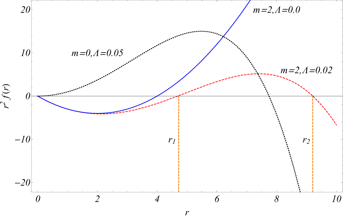
Figure 1: The function $r^{2}f(r)$ for a S-dS background metric is a decreasing function for a range of $r$ between the two horizons. Similarly for the de Sitter metric ($m=0$). In contrast for the Schwarzschild $f(r)$ is monotonically increasing.

In order to address this question we may consider an initially static field configuration $\Phi(r)$ and its rescaled form $\Phi_{\alpha}\equiv\Phi(\alpha r)$. We now search for an extremum and preferably a minimum of the energy functional (6) with respect to the scaling parameter $\alpha$. Let $E_{\alpha}$ be the energy of the rescaled field configuration

$$E_{\alpha}=4\pi\int_{r_{1}}^{r_{2}}\left[r^{2}f(r)\left(\frac{d\Phi_{\alpha}}{dr}\right)^{2}+V(\Phi_{\alpha})r^{2}\right]dr$$ (8)

Using a change of variable $r^{\prime}\equiv\alpha r$ and the facts $f(r_{1})=f(r_{2})=0$, $V(\Phi(r_{1}))=V(\Phi(r_{2}))=0$ it is straightforward to show that for the existence of a static solution a necessary condition is

$$\frac{1}{4\pi}\frac{dE}{d\alpha}\bigg{\rvert}_{\alpha=1}=I_{1}+I_{2}+I_{3}=0$$ (9)

where

$$I_{1} = -\int_{r_{1}}^{r_{2}}r^{\prime 3}f^{\prime}(r)\left(\frac{d\Phi}{dr}\right)^{2}dr$$ (10)

$$I_{2} = -\int_{r_{1}}^{r_{2}}r^{2}f(r)\left(\frac{d\Phi}{dr}\right)^{2}dr$$ (11)

$$I_{3} = -\int_{r_{1}}^{r_{2}}r^{2}\;V(\Phi)\;dr$$ (12)

Since $I_{3}<0$ and $I_{2}<0$ we need $I_{1}>0$ in order to satisfy eq. (9) and have a static solution. Thus, we need $f^{\prime}(r)<0$ at least for some range between the horizons. This condition can not be satisfied in a flat space ($f(r)=1$) and this is consistent with Derrick’s theorem. It is also not satisfied in a Schwarzschild metric ($f(r)=1-\frac{2m}{r}$) where $f(r)$ is a monotonically increasing function (Fig. 1). Thus Derrick’s theorem is also applicable for this metric (no static solution exists). A similar argumentRadmore and Stephenson (1978); Palmer (1979) exists for charged Reissner–Nordström black holes where

$$f(r)=f(r)=1-\frac{2m}{r}+\frac{e^{2}}{r^{2}}$$ (13)

In this case $r_{1}=m+\sqrt{m^{2}+e^{2}}$ and $r_{2}=+\infty$ and as in the Schwarzschild metric $f(r)$ is monotonically increasing in the integration range, leading to $I_{1}<0$ and no static solution exists.

As shown in Fig. 1, a metric for which $f(r)$ is not monotonic is the S-dS metric (eq. (7)). For this metric $f(r)$ has a maximum $f(r_{max})$ in the range $[r_{1},r_{2}]$ and is a decreasing function for $r\in[r_{max},r_{2}]$. In this range $f^{\prime}(r)<0$ and thus it is possible to have $I_{1}>0$ (static solution). Thus, Derrick’s theorem is not applicable for this metric and a static solution is allowed to exist. However such a solution is unstable for the spherical domain wall in S-dS background configuration as discussed in the next section.

In general the stability of the static solution depends on the sign of the second derivative of the energy. The necessary condition for stability is

$$\frac{d^{2}E}{d\alpha^{2}}\bigg{\rvert}_{\alpha=1}>0$$ (14)

The left hand side of this inequality depends on both the $f^{\prime}(r)$ and $f^{\prime\prime}(r)$ and thus we anticipate that for proper choice of $f(r)$ it may be satisfied leading to metastable static scalar field configuration. We thus conclude that Derrick’s theorem can be evaded in properly chosen nontrivial gravitational backgrounds.

III Spherical Domain Wall in a Schwarzschild-DeSitter Background

We now focus on the particular class of scalar field potentials that correspond to spontaneous symmetry breaking and give rise to global topological defects. The simplest topological defect, the domain wall, may form in theories where the potential $V(\Phi)$ has a discrete set of degenerate minima. Such is the double well potential leading to a spontaneous breaking of $Z_{2}$ symmetry. It is of the form

$$V(\Phi)=\frac{1}{2}\left(\Phi^{2}-\eta^{2}\right)^{2}$$ (15)

where $\eta$ is the scale of symmetry breaking. A spherical domain wall is a field configuration that interpolates between the two degenerate minima $\pm\eta$ of the potential (15) as the surface of the wall sphere in physical space is crossed. An example of such a spherically symmetric field configuration is

$$\Phi(r)=\eta\;\tanh\left[\eta\left(r-r_{0}\right)\right]$$ (16)

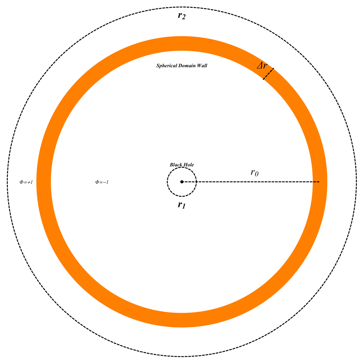
Figure 2: The geometry of the spherical domain wall described by the ansatz (16) with the presence of a S-dS black hole in its center. The horizons are also shown.

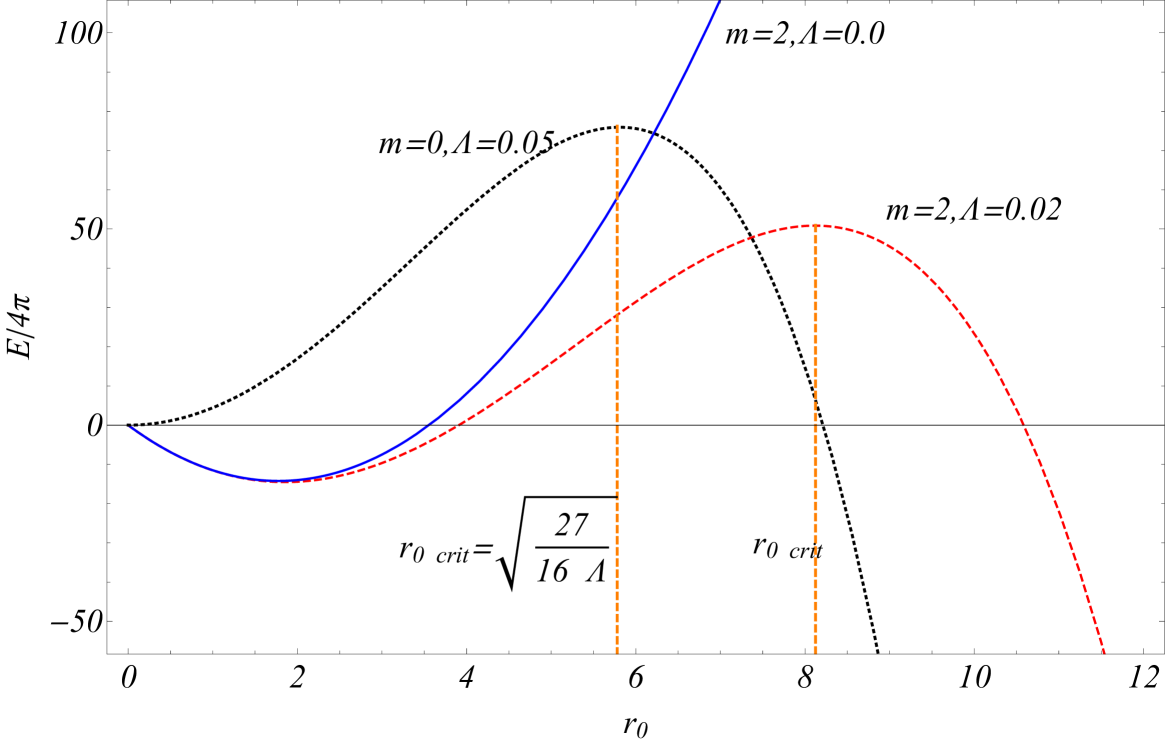
Figure 3: An approximate form of the spherical domain wall energy as a function of its radius $r_{0}$ as obtained from eq. (20).

The basic features of the evolution of this configuration describing a spherical domain wall may be obtained analytically via a simple analytical model based on an approximate form of the energy functional. They may also be obtained numerically by either explicit minimization of the full energy functional or by numerical simulation of the wall evolution by solving the dynamical equation (5) with the initial condition (16).

III.1 Analytical Model

The only scale of the model in a flat background space is the scale of symmetry breaking $\eta$ which also describes both the width $\Delta r$ of the domain wall as

$$\Delta r\simeq\eta^{-1}$$ (17)

and the scale of variation of the scalar field

$$\Delta\Phi=2\eta$$ (18)

from one vacuum to the other. The geometry of the spherical domain wall described by the ansatz (16) is shown in Fig. 1.

In what follows we rescale spacetime coordinates and energy/mass scales by the scale of symmetry breaking $\eta$. We thus set $\eta=1$ and use the rescaled dimensionless quantities.

$\begin{array}[]{@{\hspace{-0.10in}}c@{\hspace{0.0in}}c}\lx@intercol\mbox{}\hfil\lx@intercol&\lx@intercol\mbox{}\hfil\lx@intercol\\[-14.45377pt] \epsfbox{phivstbh.pdf}\hfil&\epsfbox{rvstbh.pdf}\hfil\\ \end{array}$

Figure 4: Left panel: Evolved spherical wall field configuration in flat space (black dotted line) and in the presence of a central black hole with $m=5$ $\Lambda=0$ (red line) at $t=80$. The blue line corresponds to the initial condition. Clearly the black hole delays the collapse of the wall as expected from the analytical approximate model. Right panel: The location of the zero of the scalar field (domain wall) as a function of time in the absence (black dots) and in the presence (red dots) of a central black hole. The continuous line in the black dots is a fit with a cosine harmonic function and the line in the red dots is a cosine+quadratic term in time. Due to the constant repulsive force, the black hole introduces a repulsive term quadratic in time that becomes apparent at late times.

$\begin{array}[]{@{\hspace{-0.10in}}c@{\hspace{0.0in}}c}\lx@intercol\mbox{}\hfil\lx@intercol&\lx@intercol\mbox{}\hfil\lx@intercol\\[-14.45377pt] \epsfbox{enminexp1.pdf}\hfil&\epsfbox{enmincol1.pdf}\hfil\\ \end{array}$

Figure 5: The field configuration corresponding to minimum energy is expanded to the outer boundary-horizon (left panel) if the initial guess wall radious $r_{0}$ is larger than the critical radius $r_{0crit}$ corresponding to the energy maximum of Fig. 3. Similarly, the minimum energy field configuration is collapsed to the inner boundary-horizon (right panel) if the initial guess wall radius $r_{0}$ is smaller than the critical radius $r_{0crit}$ corresponding to the energy maximum of Fig. 3. The energy minimization was performed numerically using 200 lattice points.

The evolution of the spherical domain wall (16) is described by the action (3) and the corresponding dynamical equation (5). The energy of the spherical wall, assumed initially static is given by eq. (6). Assuming a small but finite thickness of the domain wall (Fig. 2) and a S-dS background metric we may approximate its energy as

$$\frac{E}{4\pi}\simeq\left(r_{0}^{2}-2mr_{0}-\frac{\Lambda}{3}r_{0}^{4}\right)\left(\frac{\Delta\Phi}{\Delta r}\right)^{2}\Delta r+V(0)\;r_{0}^{2}\;\Delta r$$ (19)

$\begin{array}[]{@{\hspace{-0.10in}}c@{\hspace{0.0in}}c}\lx@intercol\mbox{}\hfil\lx@intercol&\lx@intercol\mbox{}\hfil\lx@intercol\\[-14.45377pt] \epsfbox{enminexp2.pdf}\hfil&\epsfbox{enmincol2.pdf}\hfil\\ \end{array}$

Figure 6: The field configuration emerging after energy minimizatio with boundary conditions imposed beyond the horizon. If the boundary conditions are imposed beyond the cosmological horizon the oscillating instabilities develop due to the negative kinetic term in the region beyond the horizon. These instabilities however do not affect the collasing/expanding properties of the field in the region where the gradient term is positive. Similar results are obtained if we use $m\neq 0$ and impose the inner boundary condition inside the black hole horizon.

Using eqs (17), (18) in (19) with $\eta\rightarrow 1$ we find

$$\frac{E}{4\pi}\simeq\frac{9}{2}r_{0}^{2}-8\;m\;r_{0}-\frac{4}{3}\Lambda\;r_{0}^{4}$$ (20)

This approximate expression for the domain wall energy as a function of its radius $r_{0}$ is shown in Fig. 3

For small values of $r_{0}$ the repulsive term proportional to the black hole mass $m$ dominates leading to a decreasing energy. For intermediate values of $r_{0}$ the tension $\sim r_{0}^{2}$ dominates leading to an increasing energy while for large wall radius the repulsive term due to the cosmological $\Lambda$ dominates and the energy becomes again a decreasing function of $r_{0}$. For $m=0$ the energy is maximised for

$$r_{0crit}=\sqrt{\frac{27}{16\Lambda}}$$ (21)

For $r_{0}>r_{0crit}$ the wall is expected to expand due to the repulsive potentials of the cosmological constant and the black hole mass while for $r_{0}<r_{0crit}$ contraction is expected due to the tension. The existence of an unstable static solution is also anticipated for $r_{0}=r_{0crit}$. Clearly, the approximate expression for the energy (20) can only by trusted in regions between the horizons where the coefficient of the gradient term remains positive.

The attractive/repulsive nature of each term is also seen via the total force applied on the domain wall due to the tension, the black hole mass and cosmological constant. This force is obtained as

$$F\equiv-\frac{\partial E}{\partial r_{0}}=-9\;r_{0}+8\;m+\frac{16}{3}\;\Lambda\;r_{0}^{3}$$ (22)

The above described predicted evolution of the spherical wall obtained using this simple analytical model is verified by numerical simulation of its evolution in the next subsection.

III.2 Numerical Derivation of Domain Wall Evolution

The repulsive potential due to the mass of the central black hole predicted by the analytical model may be verified numerically by simulating the domain wall evolution. Thus we solve the dynamical equation (5) for a S-dS background metric (7) and the symmetry breaking potential (15). In order to focus on the effects of the mass term we first set $\Lambda=0$ in eq. (7).We use the initial field configuration of eq. (16) corresponding to a spherical domain wall and boundary conditions at the two horizons

$$\Phi(r_{1}) = -1$$ (23)

$$\Phi(r_{2}) = 1$$ (24)

We evolve the configuration in time in both a flat background space ($m=0$) and in the presence of the black hole. The results are shown in Fig. 4. Clearly, the repulsive gravitational interaction originating from the black hole mass delays the collapse of the spherical wall due to its tension. The equivalence principle is not violated by this repulsive interaction since the spherical wall is a non-local object and thus the gravitational effects on it can not be eliminated at any frame.

A simple way to derive numerically the basic features of the evolution of the domain wall initial configuration (16) is to explicitly minimise the energy functional (6) with fixed boundary conditions at the two horizons $r_{1}$, $r_{2}$ corresponding to the two distinct vacua of the potential (15) (eqs (23)-(24)). We approximate the integral (6) as a discrete sum over 200 lattice points and minimize with respect to the 200 values of the field (one value at each lattice point) starting from the initial configuration (16). Thus the energy integral (6) is written as

$$E=dx\sum_{i=1}^{N}\left[r_{i}^{2}\;f(r_{i})\left(\frac{\Phi_{i}-\Phi_{i-1}}{dx}\right)^{2}+r_{i}^{2}V(\Phi_{i})\right]$$ (25)

where we have set $N=200$ and $V(\Phi_{i})$ is given by eq. (15). For simplicity we set $m=0$, $\Lambda=0.2$ in evaluating $f(r_{i})$ from eq. (7) which implies that $r_{1}=0$ and $r_{0crit}\simeq 2.9$ as obtained from eq. (21)

As expected based on the above described analytical model and the energy shown in Fig. 3, the field configuration that minimizes the energy subject to the boundary conditions (23)-(24) depends on the initial location of the domain wall (value of $r_{0}$ of the initial guess used for the minimization). For $r_{0}<r_{0crit}$ ($r_{0}>r_{0crit}$) the final field configuration corresponds to a domain wall collapsed (expanded) on the inner (outer) horizon at $r_{1}$ ($r_{2}$) where the boundary condition stops its further collapse (expansion). This effect is demonstrated in Fig. 5 which shows the initial guess wall configuration and the final configuration emerging after the energy minimization.

These results imply that there is an unstable static spherical domain wall solution for a radius $r_{0}=r_{0crit}$. The instability of this solution may also be seen by evaluating the second derivative of the energy (20) with respect to $r_{0}$ and showing that as expected it is negative at the maximum $r_{0crit}$.

If the boundary conditions (23)-(24) of the energy minimization are imposed beyond the two horizons where the field gradient term in the energy changes sign, then the expected oscillating instabilities become manifest in the regions beyond the horizons. These causally protected ghost instabilities are demonstrated in Fig. 6.

$\begin{array}[]{@{\hspace{-0.10in}}c@{\hspace{0.0in}}c}\lx@intercol\mbox{}\hfil\lx@intercol&\lx@intercol\mbox{}\hfil\lx@intercol\\[-14.45377pt] \epsfbox{pdeexp.pdf}\hfil&\epsfbox{pdecol.pdf}\hfil\\ \end{array}$

Figure 7: The numerical evolution of the spherical wall depends crucially on the initial conditions. If the initial radius $r_{0}$ is larger than the energy maximum of Fig. (3) the wall expands while if the initial radius $r_{0}$ is smaller than the energy maximum of Fig. (3) the wall contracts.

The collapsing/expanding behavior of the spherical domain wall which depends on its initial radius may also be demonstrated by explicit numerical solution of the dynamical field equation (5) in the region between the horizons with boundary conditions (23)-24) and initial condition given by eq. (16). As shown in Fig. 7 the evolution of the spherical wall depends crucially on its initial radius $r_{0}$. If $r_{0}>r_{0crit}$ the wall expands to the outer horizon while if $r_{0}<r_{0crit}$ the wall contracts towards the inner horizon. Despite of the approximations used in the analytical derivation of $r_{0crit}$ from eq. (20) we have found numerically that its value is accurate to within better than $5\%$. This is surprising in view of the significant approximations involved in deriving eq. (20).

IV Global monopole and global string loop in a S-dS spacetime

IV.1 Global Monopole in a S-dS spacetime

The analytical model introduced in section III.1 has been demonstrated to describe the qualitative features of the evolution of the spherical domain wall in the presence of a non-trivial background metric in a satisfactory manner. Motivated by this result we apply the same model in this section to obtain the gravitational interaction potential between a global monopole and a S-dS black hole.

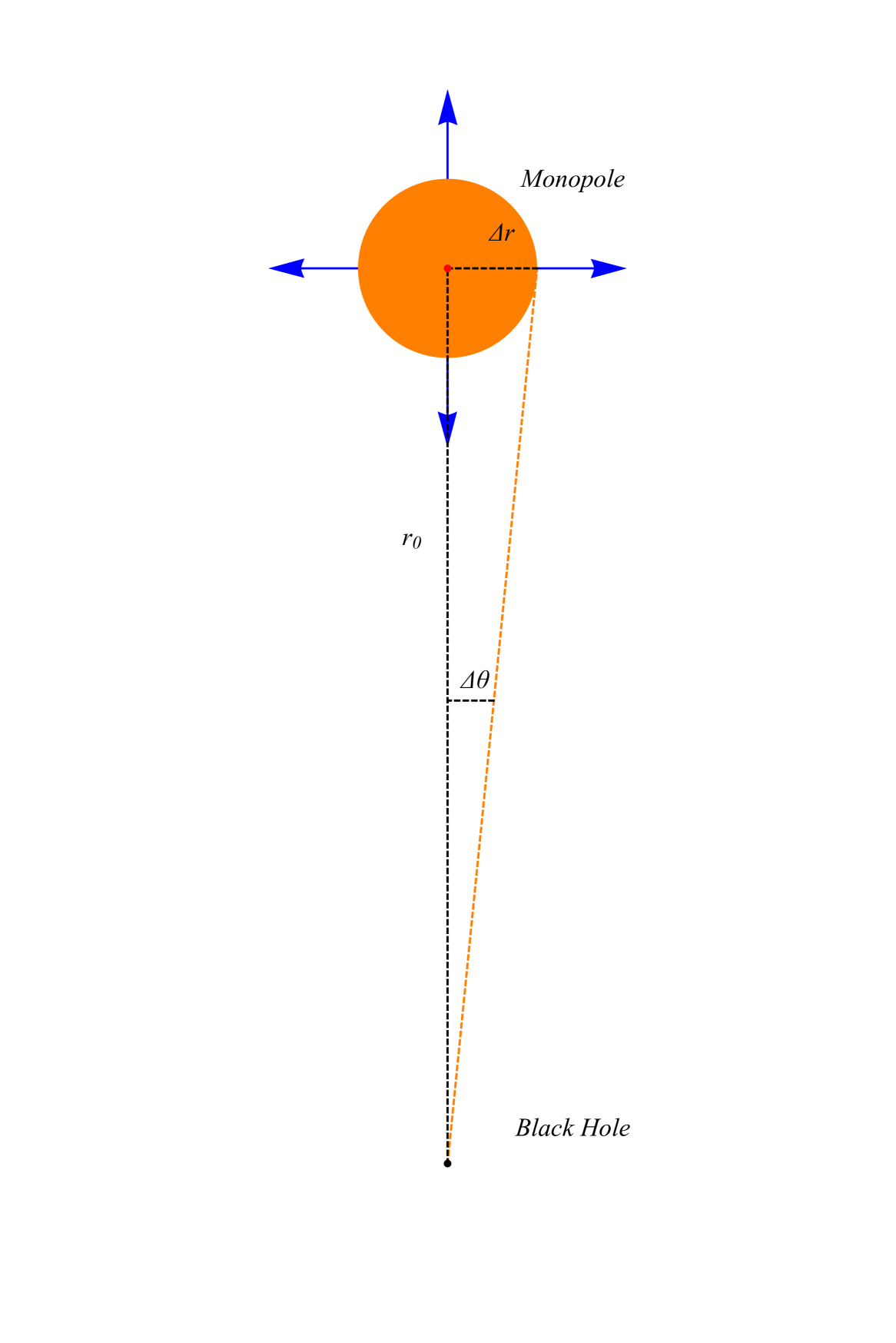
Figure 8: The global monopole as viewed from the spherical coordinate system with center on the black hole.

A global monopole with unit topological charge corresponds to a topologically stable, spherically symmetric hedgehog triplet scalar field configuration of the form

$$\Phi^{a}=\Phi(r)n^{a}$$ (26)

where $a=1,2,3$, $n^{a}\equiv(\sin\theta\cos\varphi,\sin\theta\sin\varphi,\cos\varphi)$ and the boundary conditions for $\Phi(r)$ are

$$\Phi(r=0) = 0$$ (27)

$$\Phi(r\rightarrow\infty) = 1$$ (28)

The action describing the dynamics of a global monopole is of the form

$$S=\int\left(g^{\mu\nu}\frac{\partial\Phi^{a}}{\partial x^{\mu}}\frac{\partial\Phi^{a}}{\partial x^{\nu}}-V(\sqrt{\Phi^{a}\Phi^{a}})\right)\sqrt{-g}\;d^{4}x$$ (29)

where $V(\sqrt{\Phi^{a}\Phi^{a}})=V(\Phi)$ is given by eq. (15) and in this case leads to the breaking of a global $O(3)$ symmetry to $O(2)$. The energy of the global monopole in a spherical coordinate system whose center coincides with the monopole center is

$$E=\int T_{0}^{0}\;\sqrt{-g}\;dr\;d\theta\;d\phi=\int\left[-g^{rr}(\partial_{r}\Phi)^{2}-g^{\theta\theta}(\partial_{\theta}\Phi)^{2}-g^{\theta\theta}\Phi^{2}-g^{\varphi\varphi}(\partial_{\varphi}\Phi)^{2}-g^{\varphi\varphi}\Phi^{2}\sin^{2}\theta+V(\Phi)\right]\;\sqrt{-g}\;dr\;d\theta\;d\phi$$ (30)

The terms proportional to $\Phi^{2}$ originate from the angular gradients and lead to a contribution to the energy that is independent of $r_{0}$ and would be diverging in flat space. In the S-dS spacetime where the horizons provide natural cutofs the integral of these terms is proportional to a natural cutoff scale $R_{max}$ of the S-dS spacetime provided by cosmological S-dS horizon ie

$$E_{ang}=-\int(g^{\theta\theta}\Phi^{2}+g^{\varphi\varphi}\Phi^{2}\sin^{2}\theta)\sqrt{-g}\;dr\;d\theta\;d\phi\simeq 2\int\sin\theta\;dr\;d\theta\;d\phi\sim 8\pi R_{max}$$ (31)

where $R_{max}$ is the cutoff scale of the order of the cosmological S-dS horizon $r_{2}$. The rest of the terms in the bracket of eq. (30) may be written in the form $g^{ij}\partial_{i}\Phi\partial_{j}\Phi$ which is invariant under coordinate transformations. The total energy is also invariant under a change of the origin of the coordinate system used and thus we can shift the coordinate system from the monopole center to the black hole center keeping the same expression for the energy. This configuration is shown in Fig. 8. In this shifted coordinate system, the monopole field depends on both $r$ and $\theta$ but retains its azimouthal invariance (independence from $\varphi$). Thus the energy (30) may be expressed as

$$E=2\pi\int_{r_{1}}^{r_{2}}\int_{0}^{\pi}\left[f(r)\left(\partial_{r}\Phi(r,\theta)\right)^{2}+\frac{1}{r^{2}}\left(\partial_{\theta}\Phi(r,\theta)\right)^{2}+\frac{2}{r^{2}}\Phi(r,\theta)^{2}+V(\Phi)\right]r^{2}\sin\theta dr\;d\theta$$ (32)

where $f(r)$ corresponds to the S-dS metric (eq. (7)). For a coordinate distance $r_{0}$ between the black hole and the monopole that is large compared to the scale $\Delta r\simeq\eta^{-1}$ of the monopole core ($\Delta r<<r_{0}$) the monopole energy may be approximated up to a constant diverging term proportional to $R_{max}$ (independent of $r_{0}$) as

$$E\simeq 2\pi\left[r_{0}^{2}\;f(r_{0})(\frac{\Delta\Phi}{\Delta r})^{2}+(\frac{\Delta\Phi}{\Delta\theta})^{2}+r_{0}^{2}V(0)\right]\Delta r\int_{0}^{\Delta\theta}\theta d\theta$$ (33)

where $V(0)=\frac{\eta^{4}}{2}\rightarrow\frac{1}{2}$ and we have set $\sin\theta\simeq\theta<<1$ (see Fig. 8). Also $\Delta\theta\simeq\frac{\Delta r}{r_{0}}$ is the angular scale of the global monopole core as seen from the center of the black hole. Setting $\Delta\Phi\simeq\eta\rightarrow 1$, $\Delta r\simeq\eta^{-1}\rightarrow 1$ and

$$\int_{0}^{\Delta\theta}\theta\delta\theta=\frac{\Delta\theta^{2}}{2}\simeq\frac{\Delta r^{2}}{2r_{0}^{2}}\rightarrow\frac{1}{2r_{0}^{2}}$$ (34)

we find an approximate expression for the gravitational interaction energy between monopole and black hole as

$$E\simeq\pi\left[\frac{5}{2}-\frac{2m}{r_{0}}-\frac{\Lambda}{3}r_{0}^{2}\right]$$ (35)

leading to a gravitational force on the monopole from the black hole of the form

$$F=-\frac{\partial E}{\partial r_{0}}=-\frac{2\pi Gm\eta}{r_{0}^{2}}+\frac{2\pi\Lambda\eta}{3}r_{0}$$ (36)

where we have restored $\eta$ and $G$ for clarity. Thus the monopole behaves like a point test particle with mass equal to $2\pi\eta$. As in the case of a test particle, the force consists of an attractive component due to the black hole mass (as expected from the equivalence principle) and a repulsive component from the cosmological constant. There is an unstable equilibrium point at $r_{0}=(\frac{3Gm}{\Lambda})^{1/3}$.

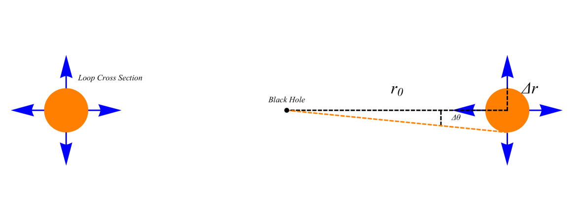
Figure 9: Cross section view of the global string loop with the central black hole.

IV.2 Global String Loop in a S-dS spacetime

The global field configuration corresponding to a global string loop is shown in Fig. 9. In this case the energy density is concentrated at $\theta\simeq\frac{\pi}{2}$ rather than $\theta\simeq 0$ and the axial symmetry remains. Setting $\sin\theta\simeq 1$ in eq. (32) and using similar approximations and arguments as in the case of the global monopole we find an approximate expression for the energy of the loop which up to a constant diverging term (independent of $r_{0}$) is of the form

$$E\simeq 2\pi\left[r_{0}^{2}\;f(r_{0})(\frac{\Delta\Phi}{\Delta r})^{2}+(\frac{\Delta\Phi}{\Delta\theta})^{2}+r_{0}^{2}V(0)\right]\Delta r\Delta\theta\simeq 2\pi\left(\frac{5}{2}r_{0}-2m-\frac{\Lambda}{3}r_{0}^{3}\right)$$ (37)

The corresponding effective force is obtained as

$$F\equiv-\frac{\partial E}{\partial r_{0}}\simeq-5\pi G\eta^{2}+2\pi G\eta^{2}\Lambda r_{0}^{2}$$ (38)

where we have restored $G$ and $\eta$ for clarity. The first term is an attractive term due to the loop tension while the second term is the repulsive term due to the cosmological constant. The black hole mass does not contribute to the effective force in this case. As in the case of the spherical domain wall we anticipate the existence of an unstable static solution for $r_{0}\simeq\sqrt{\frac{5}{2\Lambda}}$.

V Conclusion

The main results of this analysis can be summarised as follows:

• Derrick’s theorem can be violated in the presence of a non-trivial gravitational background. In fact rescaling arguments indicate that static scalar field configurations can exist in the presence of a S-dS background metric.

• A spherical domain wall in a S-dS background metric is subject to three types of potentials: a potential that favours contraction due to its tension, a potential that favours expansion due to the central black hole mass and a potential that favours expansion due to the cosmological constant. Expansion occurs for domain wall radius $r_{0}$ larger than a critical radius $r_{0crit}$ while contraction occurs $r_{0}<r_{0crit}$. This result has been demonstrated both analytically and numerically.

• A global monopole in a S-dS background metric is subject to two types of potentials: an attractive potential due to the central black hole mass and a repulsive potential due to the cosmological constant. Repulsion dominates for a monopole coordinate distance $r_{0}$ larger than a critical distance $r_{0crit}$ while attraction occurs $r_{0}<r_{0crit}$.

• A global string loop in a S-dS background metric with a central black hole is subject to two types of potentials: an attractive potential towards the central black hole due to its tension and a repulsive potential due to the cosmological constant. Repulsion dominates for a loop radius $r_{0}$ larger than a critical distance $r_{0crit}$ while attraction occurs $r_{0}<r_{0crit}$.

In all three cases of global defects interacting with a S-dS black hole we anticipate the existence of unstable static solutions for a distance (radius) from the black hole where the above effective forces vanish.

Interestingly, the mass of the central black hole acts with a repulsive force towards the spherical domain wall but with an attractive force towards a global monopole. This difference does not necessarily lead to violation of the equivalence principle since global defects are nonlocal objects. The cosmological constant acts in a repulsive manner in all three cases of defects.

Interesting extensions of the present analysis include the following:

• Extensive numerical simulations of the evolution of a global defects in the vicinity of a S-dS black hole including the cases of global string loops and global monopoles. Such simulations can lead to a more detailed study of the interaction potentials and the investigation of scattering of global defects from a S-dS black hole.

• Consideration of more general background metrics including for example a black hole-monopole or a Kerr background.

• Derivation of the predicted gravitational wave features induced by the motion of global defects in nontrivial gravitational backgrounds. Particularly interesting could be the possible gravitational wave and $\gamma$-ray bursts created during the merging of global monopoles with black holes.

• Consideration of alternative coordinate systems that may allow the more detailed investigation of the scalar field instabilities that appear to develop beyond the black hole and the cosmological horizons. This will also allow the study of the fate of the global defects as they cross the black hole horizon.

• Investigation of the deformation induced on global defect configurations by black holes located at a distance $r_{0}$ from the center of the defects.

Numerical Analysis Files: The Mathematica file used for the numerical analysis of this study and for the construction of the Figures may be downloaded from this url.

References

- Rowan and Stephenson (1976) D. J. Rowan and G. Stephenson, “Solutions of the Time Dependent Klein-Gordon Equation in a Schwarzschild Background Space,” J. Phys. A9, 1631–1635 (1976).
- Rowan and Stephenson (1977) D. J. Rowan and G. Stephenson, “The Klein-Gordon Equation in a Kerr-Newman Background Space,” J. Phys. A10, 15–23 (1977).
- Page (1976) Don N. Page, “Dirac Equation Around a Charged, Rotating Black Hole,” Phys. Rev. D14, 1509–1510 (1976).
- Mukhopadhyay and Chakrabarti (1999) Banibrata Mukhopadhyay and Sandip K. Chakrabarti, “Semianalytical solution of Dirac equation in Schwarzschild geometry,” Class. Quant. Grav. 16, 3165–3181 (1999), arXiv:gr-qc/9907100 [gr-qc] .
- Elizalde (1987) E. Elizalde, “SERIES SOLUTIONS FOR THE KLEIN-GORDON EQUATION IN SCHWARZSCHILD SPACE-TIME,” Phys. Rev. D36, 1269–1272 (1987).
- Elizalde (1988) E. Elizalde, “EXACT SOLUTIONS OF THE MASSIVE KLEIN-GORDON-SCHWARZSCHILD EQUATION,” Phys. Rev. D37, 2127–2131 (1988).
- Bezerra et al. (2014) V. B. Bezerra, H. S. Vieira, and André A. Costa, “The Klein-Gordon equation in the spacetime of a charged and rotating black hole,” Class. Quant. Grav. 31, 045003 (2014), arXiv:1312.4823 [gr-qc] .
- Vieira and Bezerra (2016) H. S. Vieira and V. B. Bezerra, “Confluent Heun functions and the physics of black holes: Resonant frequencies, Hawking radiation and scattering of scalar waves,” Annals Phys. 373, 28–42 (2016), arXiv:1603.02233 [gr-qc] .
- Sakalli (2016) I. Sakalli, “Analytical solutions in rotating linear dilaton black holes: resonant frequencies, quantization, greybody factor, and Hawking radiation,” Phys. Rev. D94, 084040 (2016), arXiv:1606.00896 [gr-qc] .
- Vieira et al. (2017) H. S. Vieira, J. P. Morais Graça, and V. B. Bezerra, “Scalar resonant frequencies and Hawking effect of an global monopole,” Chin. Phys. C41, 095102 (2017), arXiv:1705.02715 [gr-qc] .
- Kraniotis (2018) G. V. Kraniotis, “The massive Dirac equation in the curved spacetime of the Kerr-Newman (anti) de Sitter black hole,” (2018), arXiv:1801.03157 [gr-qc] .
- Bezerra et al. (2017) V. B. Bezerra, H. R. Christiansen, M. S. Cunha, and C. R. Muniz, “Exact solutions and phenomenological constraints from massive scalars in a gravity’s rainbow spacetime,” Phys. Rev. D96, 024018 (2017), arXiv:1704.01211 [gr-qc] .
- Kraniotis (2016) G. V. Kraniotis, “The Klein–Gordon–Fock equation in the curved spacetime of the Kerr–Newman (anti) de Sitter black hole,” Class. Quant. Grav. 33, 225011 (2016), arXiv:1602.04830 [gr-qc] .
- Derrick (1964) G. H. Derrick, “Comments on nonlinear wave equations as models for elementary particles,” J. Math. Phys. 5, 1252–1254 (1964).
- Radmore and Stephenson (1978) P. M. Radmore and G. Stephenson, “Nonlinear Wave Equations in a Curved Background Space,” J. Phys. A11, L149–L152 (1978).
- Palmer (1979) T.N. Palmer, “Derrick’s Theorem in Curved Space,” J. Phys. A 12, L17 (1979).
- Perivolaropoulos (1992a) Leandros Perivolaropoulos, “Nontopological global field dynamics,” Phys. Rev. D46, 1858–1862 (1992a), arXiv:hep-ph/9207256 [hep-ph] .
- Hindmarsh (1993) Mark Hindmarsh, “Semilocal topological defects,” Nucl. Phys. B392, 461–492 (1993), arXiv:hep-ph/9206229 [hep-ph] .
- Achucarro et al. (1992) Ana Achucarro, Konrad Kuijken, Leandros Perivolaropoulos, and Tanmay Vachaspati, “Dynamical simulations of semilocal strings,” Nucl. Phys. B388, 435–456 (1992).
- James et al. (1993) Margaret James, Leandros Perivolaropoulos, and Tanmay Vachaspati, “Detailed stability analysis of electroweak strings,” Nucl. Phys. B395, 534–546 (1993), arXiv:hep-ph/9212301 [hep-ph] .
- Vachaspati (1992) Tanmay Vachaspati, “Vortex solutions in the Weinberg-Salam model,” Phys. Rev. Lett. 68, 1977–1980 (1992), [Erratum: Phys. Rev. Lett.69,216(1992)].
- James et al. (1992) M. James, L. Perivolaropoulos, and T. Vachaspati, “Stability of electroweak strings,” Phys. Rev. D46, R5232–R5235 (1992).
- Perivolaropoulos (1994) Leandros Perivolaropoulos, “Stable, spinning embedded vortices,” Phys. Rev. D50, 962–966 (1994), arXiv:hep-ph/9403298 [hep-ph] .
- Achucarro and Vachaspati (2000) Ana Achucarro and Tanmay Vachaspati, “Semilocal and electroweak strings,” Phys. Rept. 327, 347–426 (2000), [Phys. Rept.327,427(2000)], arXiv:hep-ph/9904229 [hep-ph] .
- Nielsen and Olesen (1973) Holger Bech Nielsen and P. Olesen, “Vortex Line Models for Dual Strings,” Nucl. Phys. B61, 45–61 (1973), [,302(1973)].
- ’t Hooft (1974) Gerard ’t Hooft, “Magnetic Monopoles in Unified Gauge Theories,” Nucl. Phys. B79, 276–284 (1974), [,291(1974)].
- Polyakov (1974) Alexander M. Polyakov, “Particle Spectrum in the Quantum Field Theory,” JETP Lett. 20, 194–195 (1974), [,300(1974)].
- Perivolaropoulos (1993a) Leandros Perivolaropoulos, “Asymptotics of Nielsen-Olesen vortices,” Phys. Rev. D48, 5961–5962 (1993a), arXiv:hep-ph/9310264 [hep-ph] .
- Perivolaropoulos (2000) L. Perivolaropoulos, “Stabilizing textures in (3+1)-dimensions with semilocality,” Phys. Rev. D62, 047301 (2000), arXiv:hep-ph/0001181 [hep-ph] .
- Perivolaropoulos (1993b) Leandros Perivolaropoulos, “Existence of double vortex solutions,” Phys. Lett. B316, 528–533 (1993b), arXiv:hep-ph/9309261 [hep-ph] .
- Coleman (1985) Sidney R. Coleman, “Q Balls,” Nucl. Phys. B262, 263 (1985), [Erratum: Nucl. Phys.B269,744(1986)].
- Kusenko (1997) Alexander Kusenko, “Small Q balls,” Phys. Lett. B404, 285 (1997), arXiv:hep-th/9704073 [hep-th] .
- Axenides et al. (2000) Minos Axenides, Stavros Komineas, Leandros Perivolaropoulos, and Manolis Floratos, “Dynamics of nontopological solitons: Q balls,” Phys. Rev. D61, 085006 (2000), arXiv:hep-ph/9910388 [hep-ph] .
- Copeland et al. (1995) Edmund J. Copeland, M. Gleiser, and H. R. Muller, “Oscillons: Resonant configurations during bubble collapse,” Phys. Rev. D52, 1920–1933 (1995), arXiv:hep-ph/9503217 [hep-ph] .
- Bazeia et al. (2007) D. Bazeia, L. Losano, R. Menezes, and J. C. R. E. Oliveira, “Generalized Global Defect Solutions,” Eur. Phys. J. C51, 953–962 (2007), arXiv:hep-th/0702052 [hep-th] .
- Bazeia et al. (2003) D. Bazeia, J. Menezes, and R. Menezes, “New global defect structures,” Phys. Rev. Lett. 91, 241601 (2003), arXiv:hep-th/0305234 [hep-th] .
- Perivolaropoulos (1992b) Leandros Perivolaropoulos, “Instabilities and interactions of global topological defects,” Nucl. Phys. B375, 665–693 (1992b).
- Babichev (2006) E. Babichev, “Global topological k-defects,” Phys. Rev. D74, 085004 (2006), arXiv:hep-th/0608071 [hep-th] .
- Olasagasti and Vilenkin (2000) Itsaso Olasagasti and Alexander Vilenkin, “Gravity of higher dimensional global defects,” Phys. Rev. D62, 044014 (2000), arXiv:hep-th/0003300 [hep-th] .
- Gregory (2000) Ruth Gregory, “Nonsingular global string compactifications,” Phys. Rev. Lett. 84, 2564–2567 (2000), arXiv:hep-th/9911015 [hep-th] .
- Vilenkin (1985) Alexander Vilenkin, “Cosmic Strings and Domain Walls,” Phys. Rept. 121, 263–315 (1985).
- Vilenkin and Shellard (2000) A. Vilenkin and E. P. S. Shellard, Cosmic Strings and Other Topological Defects (Cambridge University Press, 2000).
- Brandenberger (1994) Robert H. Brandenberger, “Topological defects and structure formation,” Int. J. Mod. Phys. A9, 2117–2190 (1994), arXiv:astro-ph/9310041 [astro-ph] .
- Hindmarsh and Kibble (1995) M. B. Hindmarsh and T. W. B. Kibble, “Cosmic strings,” Rept. Prog. Phys. 58, 477–562 (1995), arXiv:hep-ph/9411342 [hep-ph] .
- Sakellariadou (2007) Mairi Sakellariadou, “Cosmic strings,” Proceedings, International Workshop on Quantum Simulations via Analogues: Dresden, Germany, July 25-28, 2005, Lect. Notes Phys. 718, 247–288 (2007), arXiv:hep-th/0602276 [hep-th] .
- Mermin (1979) N. D. Mermin, “The topological theory of defects in ordered media,” Rev. Mod. Phys. 51, 591–648 (1979).
- Chuang et al. (1991) Isaac Chuang, Bernard Yurke, Ruth Durrer, and Neil Turok, “Cosmology in the Laboratory: Defect Dynamics in Liquid Crystals,” Science 251, 1336–1342 (1991).
- Digal et al. (1999) Sanatan Digal, Rajarshi Ray, and Ajit M. Srivastava, “Observing correlated production of defect - anti-defects in liquid crystals,” Phys. Rev. Lett. 83, 5030 (1999), arXiv:hep-ph/9805502 [hep-ph] .
- Zurek (1996) W. H. Zurek, “Cosmological experiments in condensed matter systems,” Phys. Rept. 276, 177–221 (1996), arXiv:cond-mat/9607135 [cond-mat] .
- Bowick et al. (1994) Mark J. Bowick, L. Chandar, Eric A. Schiff, and Ajit M. Srivastava, “The Cosmological Kibble mechanism in the laboratory: String formation in liquid crystals,” 1st Iberian Meeting on Gravity (IMG-1) Evora, Portugal, September 21-26, 1992, Science 263, 943–945 (1994), arXiv:hep-ph/9208233 [hep-ph] .
- Durrer et al. (2002) R. Durrer, M. Kunz, and A. Melchiorri, “Cosmic structure formation with topological defects,” Phys. Rept. 364, 1–81 (2002), arXiv:astro-ph/0110348 [astro-ph] .
- Pen et al. (1997) Ue-Li Pen, Uros Seljak, and Neil Turok, “Power spectra in global defect theories of cosmic structure formation,” Phys. Rev. Lett. 79, 1611–1614 (1997), arXiv:astro-ph/9704165 [astro-ph] .
- Vilenkin (1981a) A. Vilenkin, “Gravitational Field of Vacuum Domain Walls and Strings,” Phys. Rev. D23, 852–857 (1981a).
- Bazeia et al. (2005) D. Bazeia, C. Furtado, and A. R. Gomes, “Gravitacional field of a global defect,” (2005), arXiv:gr-qc/0512138 [gr-qc] .
- Perivolaropoulos (2005) Leandros Perivolaropoulos, “The Rise and fall of the cosmic string theory for cosmological perturbations,” The density perturbation in the universe: Beyond the inflation paradigm. Proceedings, International Workshop on particle cosmology, Athens, Greece, June 25-26, 2005, Nucl. Phys. Proc. Suppl. 148, 128–140 (2005), arXiv:astro-ph/0501590 [astro-ph] .
- Sikivie (1982) P. Sikivie, “Of Axions, Domain Walls and the Early Universe,” Phys. Rev. Lett. 48, 1156–1159 (1982).
- Lukas et al. (1999) Andre Lukas, Burt A. Ovrut, K. S. Stelle, and Daniel Waldram, “The Universe as a domain wall,” Phys. Rev. D59, 086001 (1999), arXiv:hep-th/9803235 [hep-th] .
- Harari and Sikivie (1987) Diego Harari and P. Sikivie, “On the Evolution of Global Strings in the Early Universe,” Phys. Lett. B195, 361–365 (1987).
- Kusenko and Shaposhnikov (1998) Alexander Kusenko and Mikhail E. Shaposhnikov, “Supersymmetric Q balls as dark matter,” Phys. Lett. B418, 46–54 (1998), arXiv:hep-ph/9709492 [hep-ph] .
- Enqvist and McDonald (1998) Kari Enqvist and John McDonald, “Q balls and baryogenesis in the MSSM,” Phys. Lett. B425, 309–321 (1998), arXiv:hep-ph/9711514 [hep-ph] .
- Durrer et al. (1999) R. Durrer, M. Kunz, and A. Melchiorri, “Cosmic microwave background anisotropies from scaling seeds: Global defect models,” Phys. Rev. D59, 123005 (1999), arXiv:astro-ph/9811174 [astro-ph] .
- Bennett and Rhie (1990) D. P. Bennett and S. H. Rhie, “Cosmological evolution of global monopoles and the origin of large scale structure,” Phys. Rev. Lett. 65, 1709–1712 (1990).
- Perivolaropoulos (1992c) L. Perivolaropoulos, “Large scale structure by global monopoles and cold dark matter,” Mod. Phys. Lett. A7, 903–910 (1992c), arXiv:hep-ph/9207255 [hep-ph] .
- Pogosian and Vachaspati (1999) Levon Pogosian and Tanmay Vachaspati, “Cosmic microwave background anisotropy from wiggly strings,” Phys. Rev. D60, 083504 (1999), arXiv:astro-ph/9903361 [astro-ph] .
- Perivolaropoulos et al. (1990) Leandros Perivolaropoulos, Robert H. Brandenberger, and Albert Stebbins, “Dissipationless Clustering of Neutrinos in Cosmic String Induced Wakes,” Phys. Rev. D41, 1764 (1990).
- Perivolaropoulos (1993c) Leandros Perivolaropoulos, “COBE versus cosmic strings: An Analytical model,” Phys. Lett. B298, 305–311 (1993c), arXiv:hep-ph/9208247 [hep-ph] .
- Moessner et al. (1994) R. Moessner, L. Perivolaropoulos, and Robert H. Brandenberger, “A Cosmic string specific signature on the cosmic microwave background,” Astrophys. J. 425, 365–371 (1994), arXiv:astro-ph/9310001 [astro-ph] .
- Barriola and Vilenkin (1989) Manuel Barriola and Alexander Vilenkin, “Gravitational Field of a Global Monopole,” Phys. Rev. Lett. 63, 341 (1989).
- Harari and Lousto (1990) Diego Harari and Carlos Lousto, “Repulsive gravitational effects of global monopoles,” Phys. Rev. D42, 2626–2631 (1990).
- Hiscock (1990) William A. Hiscock, “ASTROPHYSICAL BOUNDS ON GLOBAL MONOPOLES,” Phys. Rev. Lett. 64, 344–347 (1990).
- Dando and Gregory (1998) Owen Dando and Ruth Gregory, “Global monopoles in dilaton gravity,” Class. Quant. Grav. 15, 985–995 (1998), arXiv:gr-qc/9709029 [gr-qc] .
- Barros and Romero (1997) A. Barros and C. Romero, “Global monopoles in Brans-Dicke theory of gravity,” Phys. Rev. D56, 6688–6691 (1997), arXiv:gr-qc/9707040 [gr-qc] .
- Harari and Sikivie (1988) Diego Harari and P. Sikivie, “The Gravitational Field of a Global String,” Phys. Rev. D37, 3438 (1988).
- Vilenkin (1981b) A. Vilenkin, “Cosmic Strings,” Phys. Rev. D24, 2082–2089 (1981b).
- Cohen and Kaplan (1988) Andrew G. Cohen and David B. Kaplan, “The Exact Metric About Global Cosmic Strings,” Phys. Lett. B215, 67–72 (1988).
- Csaki et al. (2000) Csaba Csaki, Joshua Erlich, Christophe Grojean, and Timothy J. Hollowood, “General properties of the selftuning domain wall approach to the cosmological constant problem,” Nucl. Phys. B584, 359–386 (2000), arXiv:hep-th/0004133 [hep-th] .
- Gremm (2000a) Martin Gremm, “Thick domain walls and singular spaces,” Phys. Rev. D62, 044017 (2000a), arXiv:hep-th/0002040 [hep-th] .
- Gremm (2000b) Martin Gremm, “Four-dimensional gravity on a thick domain wall,” Phys. Lett. B478, 434–438 (2000b), arXiv:hep-th/9912060 [hep-th] .
- Axenides and Perivolaropoulos (1997) Minos Axenides and Leandros Perivolaropoulos, “Topological defects with nonsymmetric core,” Phys. Rev. D56, 1973–1981 (1997), arXiv:hep-ph/9702221 [hep-ph] .
- Axenides et al. (1998) Minos Axenides, Leandros Perivolaropoulos, and Mark Trodden, “Phase transitions in the core of global embedded defects,” Phys. Rev. D58, 083505 (1998), arXiv:hep-ph/9801232 [hep-ph] .
- De Villiers and Frolov (1998a) Jean-Pierre De Villiers and Valeri P. Frolov, “Scattering of straight cosmic strings by black holes: Weak field approximation,” Phys. Rev. D58, 105018 (1998a), arXiv:gr-qc/9804087 [gr-qc] .
- De Villiers and Frolov (1998b) Jean-Pierre De Villiers and Valeri P. Frolov, “Gravitational capture of cosmic strings by a black hole,” Int. J. Mod. Phys. D7, 957–967 (1998b), arXiv:gr-qc/9711045 [gr-qc] .
- Lonsdale and Moss (1988) S. Lonsdale and I. Moss, “The Motion of Cosmic Strings Under Gravity,” Nucl. Phys. B298, 693–700 (1988).
- Dabrowski and Larsen (1997) Mariusz P. Dabrowski and Arne L. Larsen, “Null strings in Schwarzschild space-time,” Phys. Rev. D55, 6409–6414 (1997), arXiv:hep-th/9610243 [hep-th] .
- Dubath et al. (2007) Florian Dubath, Mairi Sakellariadou, and Claude Michel Viallet, “Scattering of cosmic strings by black holes: Loop formation,” Int. J. Mod. Phys. D16, 1311–1325 (2007), arXiv:gr-qc/0609089 [gr-qc] .
- Page (1998) Don N. Page, “Gravitational capture and scattering of straight test strings with large impact parameters,” Phys. Rev. D58, 105026 (1998), arXiv:gr-qc/9804088 [gr-qc] .
- de Vega and Egusquiza (1994) H. J. de Vega and I. L. Egusquiza, “Strings in cosmological and black hole backgrounds: Ring solutions,” Phys. Rev. D49, 763–778 (1994), arXiv:hep-th/9309016 [hep-th] .
- Frolov et al. (1989) Valeri P. Frolov, V. Skarzhinsky, A. Zelnikov, and O. Heinrich, “Equilibrium Configurations of a Cosmic String Near a Rotating Black Hole,” Phys. Lett. B224, 255–258 (1989).
- Natário et al. (2018) José Natário, Leonel Queimada, and Rodrigo Vicente, “Rotating elastic string loops in flat and black hole spacetimes: stability, cosmic censorship and the Penrose process,” Class. Quant. Grav. 35, 075003 (2018), arXiv:1712.05416 [gr-qc] .
- Christensen et al. (1998) M. Christensen, Valeri P. Frolov, and A. L. Larsen, “Soap bubbles in outer space: Interaction of a domain wall with a black hole,” Phys. Rev. D58, 085008 (1998), arXiv:hep-th/9803158 [hep-th] .
- Porfyriadis and Papadopoulos (1998) P. I. Porfyriadis and D. Papadopoulos, “Null strings in Kerr space-time,” Phys. Lett. B417, 27–32 (1998), arXiv:hep-th/9707183 [hep-th] .
- Larsen (1994) Arne L. Larsen, “Circular strings in de Sitter space-time,” in 2nd Journee Cosmologique within the framework of the International School of Astrophysics, D. Chalonge Paris, France, June 2-4, 1994 (1994) pp. 0053–85, arXiv:hep-th/9408026 [hep-th] .
- Ye and Brandenberger (1990a) Jinwu Ye and Robert H. Brandenberger, “The Formation and Evolution of Vortices in an Expanding Universe,” Mod. Phys. Lett. A5, 157 (1990a).
- Press et al. (1989) William H. Press, Barbara S. Ryden, and David N. Spergel, “Dynamical Evolution of Domain Walls in an Expanding Universe,” Astrophys. J. 347, 590–604 (1989).
- Lopez-Eiguren et al. (2017a) Asier Lopez-Eiguren, Joanes Lizarraga, Mark Hindmarsh, and Jon Urrestilla, “Cosmic Microwave Background constraints for global strings and global monopoles,” JCAP 1707, 026 (2017a), arXiv:1705.04154 [astro-ph.CO] .
- Hagmann and Sikivie (1991) C. Hagmann and P. Sikivie, “Computer simulations of the motion and decay of global strings,” Nucl. Phys. B363, 247–280 (1991).
- Ye and Brandenberger (1990b) Jinwu Ye and Robert H. Brandenberger, “The Formation and Evolution of U(1) Gauged Vortices in an Expanding Universe,” Nucl. Phys. B346, 149–159 (1990b).
- Bevis et al. (2007a) Neil Bevis, Mark Hindmarsh, Martin Kunz, and Jon Urrestilla, “CMB power spectrum contribution from cosmic strings using field-evolution simulations of the Abelian Higgs model,” Phys. Rev. D75, 065015 (2007a), arXiv:astro-ph/0605018 [astro-ph] .
- Bevis et al. (2007b) Neil Bevis, Mark Hindmarsh, Martin Kunz, and Jon Urrestilla, “CMB polarization power spectra contributions from a network of cosmic strings,” Phys. Rev. D76, 043005 (2007b), arXiv:0704.3800 [astro-ph] .
- Daverio et al. (2016) David Daverio, Mark Hindmarsh, Martin Kunz, Joanes Lizarraga, and Jon Urrestilla, “Energy-momentum correlations for Abelian Higgs cosmic strings,” Phys. Rev. D93, 085014 (2016), [Erratum: Phys. Rev.D95,no.4,049903(2017)], arXiv:1510.05006 [astro-ph.CO] .
- Lopez-Eiguren et al. (2017b) A. Lopez-Eiguren, J. Urrestilla, A. Achúcarro, A. Avgoustidis, and C. J. A. P. Martins, “Evolution of Semilocal String Networks: II. Velocity estimators,” Phys. Rev. D96, 023526 (2017b), arXiv:1704.00991 [hep-ph] .
- Hindmarsh et al. (2017) Mark Hindmarsh, Joanes Lizarraga, Jon Urrestilla, David Daverio, and Martin Kunz, “Scaling from gauge and scalar radiation in Abelian Higgs string networks,” Phys. Rev. D96, 023525 (2017), arXiv:1703.06696 [astro-ph.CO] .
- Urrestilla and Vilenkin (2008) Jon Urrestilla and Alexander Vilenkin, “Evolution of cosmic superstring networks: A Numerical simulation,” JHEP 02, 037 (2008), arXiv:0712.1146 [hep-th] .
- Ipser and Sikivie (1984) J. Ipser and P. Sikivie, “The Gravitationally Repulsive Domain Wall,” Phys. Rev. D30, 712 (1984).
- Di Casola et al. (2015) Eolo Di Casola, Stefano Liberati, and Sebastiano Sonego, “Nonequivalence of equivalence principles,” Am. J. Phys. 83, 39 (2015), arXiv:1310.7426 [gr-qc] .