A Primal-Dual Online Deterministic Algorithm for Matching with Delays

Abstract.

In the Min-cost Perfect Matching with Delays (MPMD) problem, $2m$ requests arrive over time at points of a metric space. An online algorithm has to connect these requests in pairs, but a decision to match may be postponed till a more suitable matching pair is found. The goal is to minimize the joint cost of connection and the total waiting time of all requests.

We present an $O(m)$-competitive deterministic algorithm for this problem, improving on an existing bound of $O(m^{\log_{2}{5.5}})=O(m^{2.46})$. Our algorithm also solves (with the same competitive ratio) a bipartite variant of MPMD, where requests are either positive or negative and only requests with different polarities may be matched with each other. Unlike the existing randomized solutions, our approach does not depend on the size of the metric space and does not have to know it in advance.

1. Introduction

Consider a gaming platform that hosts two-player games, such as chess, go or Scrabble, where participants are joining in real time, each wanting to play against another human player. The system matches players according to their known capabilities aiming at minimizing their dissimilarities: any player wants to compete against an opponent with comparable skills. A better match for a player can be found if the platform delays matching decisions as meanwhile more appropriate opponents may join the system. However, an excessive delay may also degrade the quality of experience. Therefore, a matching mechanism that runs on a gaming platform has to balance two conflicting objectives: to minimize the waiting time of any player and to minimize dissimilarities between matched players.

The problem informally described above, called Min-cost Perfect Matching with Delays (MPMD), has been recently introduced by Emek et al. [20]. The problem is inherently online: a matching algorithm for the gaming platform has to react in real time, without knowledge about future requests (player arrivals) and make its decision irrevocably: once two requests (players) are paired, they remain paired forever.

The MPMD problem was also considered in a bipartite variant, called Min-cost Bipartite Perfect Matching with Delays (MBPMD) introduced by Ashlagi et al. [2]. There requests have polarities: one half of them is positive, and the other half is negative. An algorithm may match only requests of different signs. This setting corresponds to a variety of real-life scenarios, e.g., assigning drivers to passengers on ride-sharing platforms or matching patients to donors in kidney transplants. Similarly to the MPMD problem, there is a trade-off between minimizing the waiting time and finding a better match (a closer driver or a more compatible donor).

1.1. Problem Definition

Formally, both in the MPMD and MBPMD problems, there is a metric space $\mathcal{X}$ equipped with a distance function $\textsf{dist}:\mathcal{X}\times\mathcal{X}\to\mathbb{R}_{\geq 0}$, both known in advance to an online algorithm. An online part of the input is a sequence of $2m$ requests $u_{1},u_{2},\ldots,u_{2m}$. A request (e.g., a player arrival) $u$ is a triple $u=(\textsf{pos}(u),\textsf{atime}(u),\textsf{sgn}(u))$, where $\textsf{atime}(u)$ is the arrival time of request $u$, $\textsf{pos}(u)\in\mathcal{X}$ is the request location, and $\textsf{sgn}(u)$ is the polarity of the request.

In the bipartite case, half of the requests are positive and $\textsf{sgn}(u)=+1$ for any such request $u$; the remaining half are negative and there $\textsf{sgn}(u)=-1$. In the non-bipartite case, requests do not have polarities, but for technical convenience we set $\textsf{sgn}(u)=0$ for any request $u$.

In applications described above, the function dist measures the dissimilarity of a given pair of requests (e.g., discrepancy between player capabilities in the gaming platform scenario or the physical distance between a driver and a passenger in the ride-sharing platform scenario). For instance, for chess, a player is commonly characterized by her Elo rating (an integer) [19]. In such case, $\mathcal{X}$ may be simply a set of all integers with the distance between two points defined as the difference of their values.

Requests arrive over time, i.e., $\textsf{atime}(u_{1})\leq\textsf{atime}(u_{2})\leq\dots\leq\textsf{atime}(u_{2m})$. We note that the integer $m$ is not known beforehand to an online algorithm. At any time $\tau$, an online algorithm may match a pair of requests (players) $u$ and $v$ that

• have already arrived ($\tau\geq\textsf{atime}(u)$ and $\tau\geq\textsf{atime}(v)$),

• have not been matched yet,

• satisfy $\textsf{sgn}(u)=-\textsf{sgn}(v)$ (i.e., have opposite polarities in the bipartite case; in the non-bipartite case, this condition trivially holds for any pair).

The cost incurred by such matching edge is then $\textsf{dist}(\textsf{pos}(u),\textsf{pos}(v))+(\tau-\textsf{atime}(u))+(\tau-\textsf{atime}(v))$. That is, it is the sum of the connection cost defined as $\textsf{dist}(\textsf{pos}(u),\textsf{pos}(v))$ and the waiting costs of $u$ and $v$, defined as $\tau-\textsf{atime}(u)$ and $\tau-\textsf{atime}(v)$, respectively.

The goal is to eventually match all requests and minimize the total cost of all matching edges. We perform worst-case analysis, assuming that the requests are given by an adversary. To measure the performance of an online algorithm Alg for an input instance $\mathcal{I}$, we compare its cost $\textsc{Alg}(\mathcal{I})$ to the cost $\textsc{Opt}(\mathcal{I})$ of an optimal offline solution Opt that knows the entire input sequence in advance. The objective is to minimize the competitive ratio [14] defined as $\sup_{\mathcal{I}}\{\textsc{Alg}(\mathcal{I})/\textsc{Opt}(\mathcal{I})\}$.

1.2. Previous Work

The MPMD problem was introduced by Emek et al. [20], who presented a randomized $O(\log^{2}n+\log\Delta)$-competitive algorithm. There, $n$ is the number of points in the metric space $\mathcal{X}$ and $\Delta$ is its aspect ratio (the ratio between the largest and the smallest distance in $\mathcal{X}$). The competitive ratio was subsequently improved by Azar et al. [4] to $O(\log n)$. They also showed that the competitive ratio of any randomized algorithm is at least $\Omega(\sqrt{\log n})$. The currently best lower bound of $\Omega(\log n/\log\log n)$ for randomized solutions was given by Ashlagi et al. [2].

Ashlagi et al. [2] adapted the algorithm of Azar et al. [4] to the bipartite setting and obtained a randomized $O(\log n)$-competitive algorithm for this variant. The currently best lower bound of $\Omega(\sqrt{\log n/\log\log n})$ for this variant was also given in [2].

Both lower bounds use $O(n)$ requests. Therefore, they imply that no randomized algorithm can achieve a competitive ratio lower than $\Omega(\log m/\log\log m)$ in the non-bipartite case and lower than $\Omega(\sqrt{\log m/\log\log m})$ in the bipartite one. (Recall that $2m$ is the number of requests in the input.)

The status of the achievable performance of deterministic solutions is far from being resolved. No better lower bounds than the ones used for randomized settings are known for deterministic algorithms. The first solution that worked for general metric spaces was given by Bienkowski et al. and achieved an embarrassingly high competitive ratio of $O(m^{\log_{2}{5.5}})=O(m^{2.46})$ [12]. Roughly speaking, their algorithm is based on growing spheres around not-yet-paired requests. Each sphere is created upon a request arrival, grows with time, and when two spheres touch, the corresponding requests become matched.

Concurrently and independently of our current paper, Azar and Jacob-Fanani [6] improved the deterministic ratio to $O((1/\varepsilon)\cdot m^{\log(3/2+\varepsilon)})$, where $\varepsilon>0$ is a parameter of their algorithm. When $\varepsilon$ is small enough, this ratio becomes $O(m^{0.59})$. Their approach is similar to that of [12], but they grow spheres in a smarter way: slower than time progresses and only in the negative direction of time axis.

Better deterministic algorithms are known only for simple spaces: Azar et al. [4] gave an $O(\textnormal{height})$-competitive algorithm for trees and Emek et al. [21] constructed a $3$-competitive deterministic solution for two-point metrics (the latter competitive ratio is best possible).

1.3. Our Contribution

In this paper, we focus on deterministic solutions for both the MPMD and MBPMD problems, i.e., for both the non-bipartite and the bipartite variants of the problem. We present a simple $O(m)$-competitive LP-based algorithm that works in both settings.

In contrast to the previous randomized solutions to these problems [2, 4, 20], and similarly to other deterministic solutions [6, 12], we do not need the metric space $\mathcal{X}$ to be finite and known in advance by an online algorithm. (All previous randomized solutions started by approximating $\mathcal{X}$ by a random HST (hierarchically separated tree) [22] or a random HST tree with reduced height [8].) This approach, which can be performed only in the randomized setting, greatly simplifies the task as the underlying tree metric reveals a lot of structural information about the cuts between points of $\mathcal{X}$ and hence about the structure of an optimal solution. In the deterministic setting, such information has to be gradually learned as time passes. For our algorithm, we require only that, together with any request $u$, it learns the distances from $u$ to all previous requests.

In contrast to the previous deterministic algorithms [6, 12], we base our algorithm on the moat-growing framework, developed originally for (offline) constrained connectivity problems (e.g., for Steiner problems) by Goemans and Williamson [24]. Glossing over a lot of details, in this framework, one writes a primal linear relaxation of the problem and its dual. The primal program has a constraint (connectivity requirement) for any subset of requests and the dual program has a variable for any such subset. The algorithm maintains a family of active sets, which are initially singletons. In the runtime, dual variables are increased simultaneously, till some dual constraint (corresponding to a pair of requests) becomes tight: in such case an algorithm connects such pair and merges the corresponding sets. At the end, an algorithm usually performs pruning by removing redundant edges.

When one tries to adapt the moat-growing framework to online setting, the main difficulty stems from the irrevocability of the pairing decision: the pruning operation performed at the end is no longer an option. Another difficulty is that an algorithm has to combine the concept of actual time that passes in an online instance with the virtual time that dictates the growth of dual variables. In particular, dual variables may only start to grow once an online algorithm learns about the request and not from the very beginning as they would do in the offline setting. Finally, requests appear online, and hence both primal and dual programs evolve in time. For instance, this means that for badly defined algorithms, appearing dual constraints may be violated already once they are introduced.

We note that $2m$ (the number of requests) is incomparable with $n$ (the number of different points in the metric space $\mathcal{X}$) and their relation depends on the application. Our algorithm is better suited for applications, where $\mathcal{X}$ is infinite or virtually infinite (e.g., it corresponds to an Euclidean plane or a city map for ride-sharing platforms [32]) or very large (e.g., for some real-time online games, where player capabilities are represented as multi-dimensional vectors describing their rank, reflex, offensive and defensive skills, etc. [3]).

1.4. Alternative Deterministic Approaches (That Fail)

A few standard deterministic approaches fail when applied to the MPMD and MBPMD problems. One such attempt is the doubling technique (see, e.g., [17]): an online algorithm may trace the cost of an optimal solution Opt and perform a global operation (e.g., match many pending requests) once the cost of Opt increases significantly (e.g., by a factor of two) since the last time when such global operation was performed. This approach does not seem to be feasible here as the total cost of Opt may decrease when new requests appear.

Another attempt is to observe that the randomized algorithm by Azar et al. [4] is a deterministic algorithm run on a random tree that approximates the original metric space. One may try to replace a random tree by a deterministically generated tree that spans requested points of the metric space. Such spanning tree can be computed by the standard greedy routine for the online Steiner tree problem [26]. However, it turns out that the competitive ratio of the resulting algorithm is $2^{\Omega(m)}$. (The main reason is that the adversary may give an initial subsequence that forces the algorithm to create a spanning tree with the worst-case stretch of $2^{\Omega(m)}$ and such initial subsequence can be served by Opt with a negligible cost. The details are given in Appendix B.)

1.5. Related Work

Originally, online metric matching problems have been studied in variants where delaying decisions was not permitted. In this variant, $m$ requests with positive polarities are given at the beginning to an algorithm. Afterwards, $m$ requests with negative polarities are presented one by one to an algorithm and they have to be matched immediately to existing positive requests. The goal is to minimize the weight of a perfect matching created by the algorithm. For general metric spaces, the best deterministic algorithms achieve the optimal competitive ratio of $2m-1$ [27, 30, 36] and the best randomized solution is $O(\log^{2}m)$-competitive [7, 34]. Better bounds are known for line metrics [1, 23, 25, 31]: here the best deterministic algorithm is $O(\log^{2}m)$-competitive [35] and the best randomized one achieves the ratio of $O(\log m)$ [25].

Another strand of research concerning online matching problems arose around a non-metric setting where points with different polarities are connected by graph edges and the goal is to maximize the cardinality or the weight of the produced matching. For a comprehensive overview of these type of problems we refer the reader to a recent survey by Mehta [33].

The M(B)PMD problem is an instance in a broader category of problems, where an online algorithm may delay its decisions, but such delays come with a certain cost. Similar trade-offs were employed in other areas of online analysis: in aggregating orders in supply-chain management [9, 10, 11, 15, 16], aggregating messages in computer networks [18, 28, 29], or recently for server problems [5, 13].

2. Primal-Dual Formulation

We start with introducing a linear program that allows us to lower-bound the cost of an optimal solution. To this end, fix an instance $\mathcal{I}$ of M(B)PMD. Let $V$ be the set of all requests. We call any unordered pair of different requests in $\mathcal{I}$ an edge; let $E$ be the set of all edges that correspond to potential matching pairs, i.e., the set of all edges in the non-bipartite case, and the edges that connect requests of opposite polarities in the bipartite variant. For each set $S\subseteq V$, by $\delta(S)$ we denote the set of all edges from $E$ crossing the boundary of $S$, i.e., having exactly one endpoint in $S$.

For any set $S\subseteq V$, we define $\textsf{sur}(S)$ (surplus of set $S$) as the number of unmatched requests in a maximum cardinality matching of requests within set $S$.

• In the non-bipartite variant (MPMD), we are allowed to match any two requests. Hence, if $S$ is of even size, then $\textsf{sur}(S)=0$. Otherwise, $\textsf{sur}(S)=1$ as in any maximum cardinality matching of requests within $S$ exactly one request remains unmatched.

• In the bipartite variant (MBPMD), we can always match two requests of different polarities. Hence, the surplus of a set $S$ is the discrepancy between the number of positive and negative requests inside $S$, i.e., $\textsf{sur}(S)=|\sum_{u\in S}\textsf{sgn}(u)|$.

To describe a matching, we use the following notation. For each edge $e$, we introduce a binary variable $x_{e}$, such that $x_{e}=1$ if and only if $e$ is a matching edge. For any set $S\subseteq V$ and any feasible matching (in particular the optimal one), it holds that $\sum_{e\in\delta(S)}x_{e}\geq\textsf{sur}(S)$.

Fix an optimal solution Opt for $\mathcal{I}$. If a pair of requests $e=(u,v)$ is matched by Opt, it is matched as soon as both $u$ and $v$ arrive, and hence the cost of matching $u$ with $v$ in the solution of Opt is equal to $\textsf{opt-cost}(e):=\textsf{dist}(\textsf{pos}(u),\textsf{pos}(v))+|\textsf{atime}{(u)}-\textsf{atime}{(v)}|$. This, together with the preceding observations, motivates the following linear program $\mathcal{P}$:

minimize $$\sum_{e\in E}\textsf{opt-cost}(e)\cdot x_{e}$$

subject to $$\sum_{e\in\delta(S)}x_{e}\geq\textsf{sur}(S) \quad\forall{S\subseteq V}$$

$$x_{e}\geq 0 \quad\forall e\in E.$$

As any matching is a feasible solution to $\mathcal{P}$, the cost of the optimal solution of $\mathcal{P}$ lower-bounds the cost of the optimal solution for instance $\mathcal{I}$ of M(B)PMD. Note that there might exist a feasible integral solution of $\mathcal{P}$ that does not correspond to any matching. To exclude all such solutions, we could add constraints $\sum_{e\in\delta(S)}x_{e}=1$ for all singleton sets $S$. The resulting linear program would then exactly describe the matching problem (cf. Chapter 25 of [37]). However, our main concern is not $\mathcal{P}$, but its dual and its current shape is sufficient for our purposes. The program $\mathcal{D}$, dual to $\mathcal{P}$, is then

maximize $$\sum_{S\subseteq V}\textsf{sur}(S)\cdot y_{S}$$

subject to $$\sum_{S:e\in\delta(S)}y_{S}\leq\textsf{opt-cost}(e) \quad\forall{e\in E}$$

$$y_{S}\geq 0 \quad\forall{S}\subseteq V.$$

Note that in any solution, the dual variables $y_{S}$ corresponding to sets $S$ for which $\textsf{sur}(S)=0$, can be set to $0$ without changing feasibility or objective value.

The following lemma is an immediate consequence of weak duality.

Lemma 2.1.

Fix any instance $\mathcal{I}$ of the M(B)PMD problem. Let $\textsc{Opt}(\mathcal{I})$ be the value of any optimal solution of $\mathcal{I}$ and $D$ be the value of any feasible solution of $\mathcal{D}$. Then $\textsc{Opt}(\mathcal{I})\geq D$.

Proof 2.2.

Let $P^{*}$ and $D^{*}$ be the values of optimal solutions for $\mathcal{P}$ and $\mathcal{D}$, respectively. Since any matching is a feasible solution for $\mathcal{P}$, $\textsc{Opt}(\mathcal{I})\geq P^{*}$. Hence, $\textsc{Opt}(\mathcal{I})\geq P^{*}\geq D^{*}\geq D$.

Lemma 2.1 motivates the following approach: We construct an online algorithm Greedy Dual (GD), which, along with its own solution, maintains a feasible solution $D$ for $\mathcal{D}$ corresponding to the already seen part of the input instance. This feasible dual solution not only yields a lower bound on the cost of the optimal matching, but also plays a crucial role in deciding which pair of requests should be matched.

Note that since the requests arrive in an online manner, $\mathcal{D}$ evolves in time. When a request arrives, the number of subsets of $V$ increases (more precisely, it doubles), and hence more dual variables $y_{S}$ are introduced. Moreover, the newly arrived request creates an edge with every existing request and the corresponding dual constraints are introduced. Therefore, showing the feasibility of the created dual solution is not immediate; we deal with this issue in Section 4.

3. Algorithm Greedy Dual

The high-level idea of our algorithm is as follows: Greedy Dual (GD) resembles moat-growing algorithms for solving constrained forest problems [24]. During its runtime, GD partitions all the requests that have already arrived into active sets. If an active set contains any free requests, we call this set growing, and non-growing otherwise. At any time, for each active growing set $S$, the algorithm increases continuously its dual variable $y_{S}$ until a constraint in $\mathcal{D}$ corresponding to some edge $(u,v)$ becomes tight. When it happens, GD makes both active sets (containing $u$ and $v$, respectively) inactive, and the set being their union active. In addition, if this happened due to two growing sets, GD matches as many pairs of free requests in these sets as possible: in the non-bipartite variant GD matches exactly one pair of free requests, while in the bipartite variant, GD matches free requests of different polarities until all remaining free requests have the same sign.

3.1. Algorithm Description

More precisely, at any time, GD partitions all requests that arrived until that time into active sets. It maintains mapping $\mathcal{A}$, which assigns an active set to each such request. An active set $S$, whose all requests are matched is called non-growing. Conversely, an active set $S$ is called growing if it contains at least one free request. GD ensures that the number of free requests in an active set $S$ is always equal to $\textsf{sur}(S)$. We denote the set of free requests in an active set $S$ by $\textsf{free}(S)$; if $S$ is non-growing, then $\textsf{free}(S)=\emptyset$.

When a request $u$ arrives, the singleton $\{u\}$ becomes a new active and growing set, i.e., $\mathcal{A}(u)=\{u\}$. The dual variables of all active growing sets are increased continuously with the same rate in which time passes. This increase takes place until a dual constraint between two active sets becomes tight, i.e., until there exists at least one edge $e=(u,v)$, such that

$$\mathcal{A}(u)\neq\mathcal{A}(v)\quad\text{ and }\sum_{S:e\in\delta(S)}y_{S}=\textsf{opt-cost}(e).$$ (1)

In such case, while there exists an edge $e=(u,v)$ satisfying (1), GD processes such edge in the following way. First, it merges active sets $\mathcal{A}(u)$ and $\mathcal{A}(v)$. By merging we mean that the mapping $\mathcal{A}$ is adjusted to the new active set $S=\mathcal{A}(u)\uplus\mathcal{A}(v)$ for each request of $S$. Old active sets $\mathcal{A}(u)$ and $\mathcal{A}(v)$ become inactive. Second, as long as there is a pair of free requests $u^{\prime},v^{\prime}\in S$ that can be matched with each other, GD matches them.

In the non-bipartite variant, GD matches at most one pair as each active set contains at most one free request. In the bipartite variant, GD matches pairs of free requests until all unmatched requests in $S$ (possibly zero) have the same polarity. Observe that in either case, the number of free requests after merge is equal to $\textsf{sur}(S)$. Finally, GD marks edge $e$. Marked edges are used in the analysis, to find a proper charging of the connection cost to the cost of the produced solution for $\mathcal{D}$. The pseudocode of GD is given in Algorithm 1 and an example execution that shows a partition of requests into active sets is given in Figure 1.

Algorithm 1 Algorithm Greedy Dual

1:Request arrival event:

2:     if a request $u$ arrives then

3:         $\mathcal{A}(u)\leftarrow\{u\}$

4:         for all sets $S$ such that $u\in S$ do

5:              $y_{S}\leftarrow 0$ $\triangleright$ initialize dual variables for sets containing $u$               

6:

7:Tight constraint event:

8:     while exists a tight dual constraint for edge $e=(u,v)$ where $\mathcal{A}(u)\neq\mathcal{A}(v)$ do

9:         $S\leftarrow\mathcal{A}(u)\uplus\mathcal{A}(v)$ $\triangleright$ merge two active sets

10:         for all $w\in S$ do $\triangleright$ adjust assignment $\mathcal{A}$ for the new active set $S$

11:              $\mathcal{A}(w)\leftarrow S$          

12:         mark edge $e$

13:         while there are $u^{\prime},v^{\prime}\in\textsf{free}(S)$ such that $\textsf{sgn}(u^{\prime})=-\textsf{sgn}(v^{\prime})$ do

14:              match $u^{\prime}$ with $v^{\prime}$ $\triangleright$ match as many pairs as possible               

15:

16:None of the above events occurs:

17:     for all growing active sets $S$ do

18:         increase continuously $y_{S}$ with the same rate in which time passes      

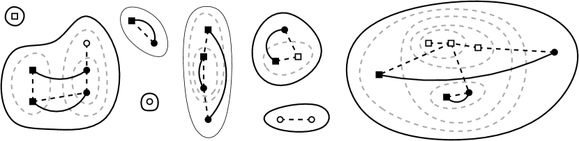
Figure 1. A partition of requests into active sets created by GD. Different polarities of requests are represented by discs and squares. Free requests are depicted as empty discs and squares, matched requests by filled ones. Active growing sets have bold boundaries and each of them contains at least one free request. Active non-growing sets contain only matched requests. Dashed lines represent marked edges and solid curvy lines represent matching edges. Dashed gray sets are already inactive; the inactive singleton sets have been omitted.

3.2. Greedy Dual Properties

It is instructive to trace how the set $\mathcal{A}(u)$ changes in time for a request $u$. At the beginning, when $u$ arrives, $\mathcal{A}(u)$ is just the singleton set $\{u\}$. Then, the set $\mathcal{A}(u)$ is merged at least once with another active set. If $\mathcal{A}(u)$ is merged with a non-growing set, the number of requests in $\mathcal{A}(u)$ increases, but its surplus remains intact. After $\mathcal{A}(u)$ is merged with a growing set, some requests inside the new $\mathcal{A}(u)$ may become matched. It is possible that, in effect, the surplus of the new set $\mathcal{A}(u)$ is zero, in which case the new set $\mathcal{A}(u)$ is non-growing. (In the non-bipartite variant, this is always the case when two growing sets merge.) After $\mathcal{A}(u)$ becomes non-growing, another growing set may be merged with $\mathcal{A}(u)$, and so on. Thus, the set $\mathcal{A}(u)$ can change its state from growing to non-growing (and back) multiple times.

The next observation summarizes the process described above, listing properties of GD that we use later in our proofs.

Observation 3.1.

The following properties hold during the runtime of GD.

1. For a request $u$, when time passes, $\mathcal{A}(u)$ refers to different active sets that contain $u$.

2. At any time, every request is contained in exactly one active set. If this request is free, then the active set is growing.

3. At any time, an active set $S$ contains exactly $\textsf{sur}(S)$ free requests.

4. Active and inactive sets together constitute a laminar family of sets.

5. For any two requests $u$ and $v$, once $\mathcal{A}(u)$ becomes equal to $\mathcal{A}(v)$, they will be equal forever.

4. Correctness

We now prove that Greedy Dual is defined properly. In other words, we show that the dual values maintained by GD always form a feasible solution of $\mathcal{D}$ (Lemma 4.3) and GD returns a feasible matching of all requests at the end (Lemma 4.5). From now on, we denote the values of a dual variable $y_{S}$ at time $\tau$ by $y_{S}(\tau)$.

By the definition, the waiting cost of a request is the time difference between the time it arrives and the time it is matched. In the following lemma, we relate the waiting cost of a request to the dual variables for the active sets it belongs to.

Lemma 4.1.

Fix any request $u$. For any time $\tau\geq\textsf{atime}(u)$, it holds that

$$\sum_{S:u\in S}y_{S}(\tau)\leq\tau-\textsf{atime}(u).$$

The relation holds with equality if $u$ is free at time $\tau$.

Proof 4.2.

We show that the inequality is preserved as time passes. At time $\tau=\textsf{atime}(u)$, request $u$ is introduced and sets $S$ containing $u$ appear. Their $y_{S}$ values are initialized to $0$. Therefore, at that time, $\sum_{S:u\in S}y_{S}(\tau)=0$ as desired.

Whenever a merging event or an arrival of any other requests occur, new variables $y_{S}$ may appear in the sum $\sum_{S:u\in S}y_{S}(\tau)$, but, at these times, the values of these variables are equal to zero, and therefore do not change the sum value.

It remains to analyze the case when time passes infinitesimally by $\varepsilon$ and no event occurs within this period. It is sufficient to argue that the sum $\sum_{S:u\in S}y_{S}(\tau)$ increases exactly by $\varepsilon$ if $u$ is free at $\tau$ and at most by $\varepsilon$ otherwise. Recall that $y_{S}$ may grow only if $S$ is an active growing set. By Property 2 of Observation 3.1, the only active set containing $u$ is $\mathcal{A}(u)$. This set is growing if $u$ is free (and then $y_{\mathcal{A}(u)}$ increases exactly by $\varepsilon$) and may be growing or non-growing if $u$ is matched (and then $y_{\mathcal{A}(u)}$ increases at most by $\varepsilon$).

The following lemma shows that throughout its runtime, GD maintains a feasible dual solution.

Lemma 4.3.

At any time, the values $y_{S}$ maintained by the algorithm constitute a feasible solution to $\mathcal{D}$.

Proof 4.4.

We show that no dual constraint is ever violated during the execution of GD.

When a new request $u$ arrives at time $\tau=\textsf{atime}(u)$, new sets containing $u$ appear and the dual variables $y_{S}$ corresponding to these sets are initialized to $0$.

Each already existing constraint, corresponding to an edge $e$ not incident to $u$, is modified: new $y_{S}$ variables for sets $S$ containing both $u$ and exactly one of endpoints of $e$ appear in the sum. However, all these variables are zero, and hence the feasibility of such constraints is preserved.

Moreover, for any edge $e=(u,v)$ where $v$ is an existing request, a new dual constraint for this edge appears in $\mathcal{D}$. We show that it is not violated, i.e., $\sum_{S:e\in\delta(S)}y_{S}(\tau)\leq\textsf{opt-cost}(e)$. As discussed before, $y_{S}(\tau)=0$ for the sets $S$ containing $u$. Therefore,

$$\sum_{S:e\in\delta(S)}y_{S}(\tau) =\sum_{S:v\in S\wedge u\notin S}y_{S}(\tau)+\sum_{S:u\in S\wedge v\notin S}y_{S}(\tau)$$

$$=\sum_{S:v\in S\wedge u\notin S}y_{S}(\tau)\leq\sum_{S:v\in S}y_{S}(\tau)$$

$$\leq\textsf{atime}(u)-\textsf{atime}(v)$$ (by Lemma 4.1)

$$\leq\textsf{opt-cost}(e).$$

Now, we prove that once a dual constraint for an edge $e=(u,v)$ becomes tight, the involved $y_{S}$ values are no longer increased. According to the algorithm definition, $\mathcal{A}(u)$ and $\mathcal{A}(v)$ become merged together. By Property 5 of Observation 3.1, from this moment on, any active set $S$ contains either both $u$ and $v$ or neither of them. Hence, there is no active set $S$, such that $(u,v)\in\delta(S)$, and in particular there is no such active growing set. Therefore, the value of $\sum_{S:e\in\delta(S)}y_{S}$ remains unchanged, and hence the dual constraint corresponding to edge $e$ remains tight and not violated.

Finally, we prove that GD returns a proper matching. We need to show that if a pair of requests remains unmatched, then appropriate dual variables increase and they will eventually trigger the matching event.

Lemma 4.5.

For any input for the M(B)PMD problem, GD returns a feasible matching.

Proof 4.6.

Suppose for a contradiction that GD does not match some request $u$. Then, by Property 2 of Observation3.1, $\mathcal{A}(u)$ is always an active growing set and by Property 3, $\textsf{sur}(\mathcal{A}(u))>0$. Therefore, the corresponding dual variable $y_{\mathcal{A}(u)}$ always increases during the execution of GD and appears in the objective function of $\mathcal{D}$ with a positive coefficient. By Lemma 4.3, the solution of $\mathcal{D}$ maintained by GD is always feasible, and hence the optimal value of $\mathcal{D}$ would be unbounded. This would be a contradiction, as there exists a finite solution to the primal program $\mathcal{P}$ (as all distances in the metric space are finite).

5. Cost Analysis

In this section, we show how to relate the cost of the matching returned by Greedy Dual to the value of the produced dual solution. First, we show that the total waiting cost of the algorithm is equal to the value of the dual solution. Afterwards, we bound the connection cost of GD by $2m$ times the dual solution, where $2m$ is the number of requests in the input. This, along with Lemma 2.1, yields the competitive ratio of $2m+1$.

5.1. Waiting Cost

In the proof below, we link the generated waiting cost with the growth of appropriate dual variables. To this end, suppose that a set $S$ is an active set for time period of length $\Delta t$. By Property 3 of Observation 3.1, $S$ contains exactly $\textsf{sur}(S)$ free points, and thus the waiting cost incurred within this time by requests in $S$ is $\Delta t\cdot\textsf{sur}(S)$. Moreover, in the same time interval, the dual variable $y_{S}$ increases by $\Delta t$, which contributes the same amount, $\textsf{sur}(S)\cdot\Delta t$, to the growth of the objective function of $\mathcal{D}$. The following lemma formalizes this observation and applies it to all active sets considered by GD in its runtime.

Lemma 5.1.

The total waiting cost of GD is equal to $\sum_{S\subseteq V}\textsf{sur}(S)\cdot y_{S}(T)$, where $T$ is the time when GD matches the last request.

Proof 5.2.

We define $G(\tau)$ as the family of sets that are active and growing at time $\tau$. By Property 2 and Property 3 of Observation 3.1, the number of free requests at time $\tau$, henceforth denoted $\textsf{wait}(\tau)$, is then equal to $\sum_{S}\textsf{sur}(S)\cdot\mathds{1}[S\in G(\tau)]$. The total waiting cost at time $T$ can be then expressed as

$$\int_{0}^{T}\textsf{wait}(\tau)\,\mathrm{d}\tau =\int_{0}^{T}\sum_{S}\textsf{sur}(S)\cdot\mathds{1}[S\in G(\tau)]\,\mathrm{d}\tau$$

$$=\sum_{S}\textsf{sur}(S)\int_{0}^{T}\mathds{1}[S\in G(\tau)]\,\mathrm{d}\tau=\sum_{S}\textsf{sur}(S)\cdot y_{S}(T),$$

where the last equality holds as at any time, GD increases $y_{S}$ value if and only if $S$ is active and growing.

5.2. Connection Cost

Below, we relate the connection cost of GD to the value of the final solution of $\mathcal{D}$, created by GD. We focus on the set of marked edges, which are created by GD in Line 12 of Algorithm 1. We show that for any time, the set of marked edges restricted to an active or an inactive set $S$ forms a “spanning tree” of requests of $S$. That is, there is a unique path of marked edges between any two requests from $S$. (Note that this path projected to the metric space may contain cycles as two requests may be given at the same point of $\mathcal{X}$.) We start with a helper observation.

Observation 5.3.

Fix any set $S$. If $S$ is active at time $\tau$, then its boundary $\delta(S)$ does not contain any marked edge at time $\tau$.

Proof 5.4.

After an edge $(u,v)$ becomes marked, both $u$ and $v$ belong to newly created active set. From now on, by Property 5 of Observation 3.1, they remain in the same active set till the end of the execution. Therefore, this edge will never be contained in a boundary of an active set.

Lemma 5.5.

At any time, for any active or inactive set $S$, the subset of all marked edges with both endpoints in $S$ forms a spanning tree of all requests from $S$.

Proof 5.6.

We show that the property holds at time passes. When a new request arrives, a new active growing set containing only one request is created. This set is trivially spanned by an empty set of marked edges.

By the definition of GD, a new active set appears when a dual constraint for some edge $e=(u,v)$ becomes tight. Right before it happens, the active sets containing $u$ and $v$ are $\mathcal{A}(u)$ and $\mathcal{A}(v)$, respectively. At that time, marked edges form spanning trees of sets $\mathcal{A}(u)$ and $\mathcal{A}(v)$ and, by Observation 5.3, there are no marked edges between these two sets. Hence, these spanning trees together with the newly marked edge $e$ constitute a spanning tree of the requests of $S=\mathcal{A}(u)\uplus\mathcal{A}(v)$. Finally, a set may become inactive only if it was active before, and GD never adds any marked edge inside an already existing active or inactive set.

Using the lemma above, we are ready to bound the connection cost of one matching edge by the cost of the solution of $\mathcal{D}$.

Lemma 5.7.

The connection cost of any matching edge is at most $2\cdot\sum_{S\subseteq V}\textsf{sur}(S)\cdot y_{S}(T)$, where $T$ is the time when GD matches the last request.

Proof 5.8.

Fix a matching edge $(u,v)$ created by GD at time $\tau$. Its connection cost is the distance $\textsf{dist}(\textsf{pos}(u),\textsf{pos}(v))$ between the points corresponding to requests $u$ and $v$ in the underlying metric space.

We consider the state of GD right after it matches $u$ with $v$. By Lemma 5.5, the active set $S=\mathcal{A}(u)=\mathcal{A}(v)$ containing $u$ and $v$ is spanned by a tree of marked edges. Let $P$ be the (unique) path in this tree connecting $u$ with $v$. Using the triangle inequality, we can bound $\textsf{dist}(\textsf{pos}(u),\textsf{pos}(v))$ by the length of $P$ projected onto the underlying metric space.

Recall that for any edge $e=(w,w^{\prime})$, it holds that $\textsf{dist}(\textsf{pos}(w),\textsf{pos}(w^{\prime}))\leq\textsf{opt-cost}(e)$. Moreover, if $e$ is marked, the dual constraint for edge $e$ holds with equality, that is, $\textsf{opt-cost}(e)=\sum_{S:e\in\delta(S)}y_{S}(\tau)$. Therefore,

$$\textsf{dist}(\textsf{pos}(u),\textsf{pos}(v)) \leq\sum_{(w,w^{\prime})\in P}\textsf{dist}(\textsf{pos}(w),\textsf{pos}(w^{\prime}))\leq\sum_{e\in P}\textsf{opt-cost}(e)$$

$$=\sum_{e\in P}\sum_{S:e\in\delta(S)}y_{S}(\tau)=\sum_{S}|\delta(S)\cap P|\cdot y_{S}(\tau)$$

$$\leq\sum_{S}|\delta(S)\cap P|\cdot\textsf{sur}(S)\cdot y_{S}(\tau)$$

$$\leq\sum_{S}|\delta(S)\cap P|\cdot\textsf{sur}(S)\cdot y_{S}(T).$$

The penultimate inequality holds because a dual variable $y_{S}$ can be positive only if $\textsf{sur}(S)\geq 1$. It is now sufficient to prove that for each (active or inactive) set $S$, it holds that $|\delta(S)\cap P|\leq 2$, i.e., the path $P$ crosses each such set $S$ at most twice.

For a contradiction, suppose that there exists an (active or inactive) set $S$, whose boundary is crossed by path $P$ more than twice. We direct all edges on $P$ towards $v$ (we follow $P$ starting from request $u$ and move towards $v$). Note that $u$ may be inside or outside of $S$. Let $e_{1}=(w_{1},w_{2})$ be the first edge on $P$ such that $w_{1}\in S$ and $w_{2}\not\in S$, i.e., the first time when path $P$ leaves $S$. Let $e_{2}=(w_{3},w_{4})\in P$ be the first edge after $e_{1}$, such that $w_{3}\not\in S$ and $w_{4}\in S$, that is, the first time when path $P$ returns to $S$ after leaving it with edge $e_{1}$. Edge $e_{2}$ must exist as we assumed that $P$ crosses the boundary of $S$ at least three times.

By Lemma 5.5, a subset of the marked edges constitutes a spanning tree of $S$. Hence, there exists a path of marked edges contained entirely in $S$ that connects requests $w_{1}$ and $w_{4}$. Furthermore, a sub-path of $P$ connects $w_{2}$ and $w_{3}$ outside of $S$. These two paths together with edges $e_{1}$ and $e_{2}$ form a cycle of marked edges. However, by Lemma 5.5 and Observation 5.3, at any time, the set of marked edges forms a forest, which is a contradiction.

5.3. Bounding the Competitive Ratio

Using above results we are able to bound the cost of Greedy Dual.

Theorem 5.9.

Greedy Dual is $(2m+1)$-competitive for the M(B)PMD problem.

Proof 5.10.

Fix any input instance $\mathcal{I}$ and let $\mathcal{D}$ be the corresponding dual program. Let $D$ be the cost of the solution to $\mathcal{D}$ output by GD. By Lemma 5.1, the total waiting cost of the algorithm is bounded by $D$ and by Lemma 5.7, the connection cost of a single edge in the matching is bounded by $2\cdot D$. Therefore,

$$\textsc{GD}(\mathcal{I})\leq D+m\cdot 2D=(2m+1)\cdot D\leq(2m+1)\cdot\textsc{Opt}(\mathcal{I}),$$

where the first inequality holds as there are exactly $m$ matched edges and the last equality follows by Lemma 2.1.

Appendix A Tightness of the Analysis

We can show that our analysis of Greedy Dual is asymptotically tight, i.e., the competitive ratio of Greedy Dual is $\Omega(m)$.

Theorem A.1.

Both for MPMD and MBPMD problems, there exists an instance $\mathcal{I}$, such that $\textsc{GD}(\mathcal{I})=\Omega(m)\cdot\textsc{Opt}(\mathcal{I})$.

Proof A.2.

Let $m>0$ be an even integer and $\varepsilon=1/m$. Let $\mathcal{X}$ be the metric containing two points $p$ and $q$ at distance $2$.

In the instance $\mathcal{I}$, requests are released at both points $p$ and $q$ at times $0,1+\varepsilon,1+3\varepsilon,1+5\varepsilon,\ldots,1+(2m-3)\cdot\varepsilon$. For the MBPMD problem, we additionally specify request polarities: at $p$, all odd-numbered requests are positive and all even-numbered are negative, while requests issued at $q$ have exactly opposite polarities from those at $p$.

Regardless of the variant (bipartite or non-bipartite) we solve, GD matches the first pair of requests at time $1$, when their active growing sets are merged, forming a new active non-growing set. Every subsequent pair of requests appears exactly $\varepsilon$ after the previous pair becomes matched. Therefore, they are matched together $\varepsilon$ after their arrival, when their growing sets are merged with the large non-growing set containing all the previous pairs of requests. Hence, the total connection cost of GD is equal to $2m$. On the other hand, observe that the total cost of a solution that matches consecutive requests at each point of the metric space separately is equal to $2\cdot((1+\varepsilon)+2\varepsilon\cdot(m-2)/2)=2\cdot(1+(m-1)\cdot\varepsilon)<4$.

Appendix B Derandomization Using a Spanning Tree

In this part, we analyze an algorithm that approximates the metric space by a greedily and deterministically chosen spanning tree of requested points and employs the deterministic algorithm for trees of Azar et al. [4]. We show that such algorithm has the competitive ratio of $2^{\Omega(m)}$. For simplicity, we focus on the non-bipartite variant, but the lower bound can be easily extended to the bipartite case.

More precisely, we define a natural algorithm Tree Based (TB). TB internally maintains a spanning tree $T$ of metric space points corresponding to already seen requests. That is, whenever TB receives a request $u$ at point $\textsf{pos}(u)$, it executes the following two steps.

1. If there was no previous request at $\textsf{pos}(u)$, TB adds $\textsf{pos}(u)$ to $T$, connecting it to the closest point from $T$. The addition is performed immediately, at the request arrival. This part essentially mimics the behavior of the greedy algorithm for the online Steiner tree problem [26].

2. To serve the request $u$, TB runs the deterministic algorithm of [4] on the tree $T$.

Theorem B.1.

The competitive ratio of Tree Based is $2^{\Omega(m)}$.

Proof B.2.

The idea of the lower bound is as follows. The adversary first gives $m/2$ requests that force TB to create a tree $T$ with the stretch of $2^{\Omega(m)}$ and then gives another $m/2$ requests, so that the initial $m$ requests can be served with a negligible cost by Opt. Afterwards, the adversary consecutively requests a pair of points that are close in the metric space, but far away in the tree $T$.

Our metric space $\mathcal{X}$ is a continuous ring and we assume that $m$ is an even integer. Let $h$ be the length of this ring and let $\varepsilon=h/(m\cdot 2^{m-1})$.

In the first part of the input, the adversary gives $m/2$ requests in the following way. The first two requests are given at time $0$ at antipodal points (their distance is $h/2$). TB connects them using one of two halves of the ring. From now on, the tree $T$ of TB will always cover a contiguous part of the ring. Each of the next $m/2-2$ requests is given exactly in the middle of the ring part not covered by $T$. For $j\in\{3,4,\ldots,m/2\}$, the $j$-th request is given at time $(2\cdot(j-1)/m)\cdot\varepsilon$.

This way, the ring part not covered by $T$ shrinks exponentially, and after $m/2$ initial requests its length is equal to $h/2^{m/2-1}$. Let $p$ and $q$ be the endpoints (the only leaves) of $T$. Then, $\textsf{dist}(p,q)=h/2^{m/2-1}$, but the path between $p$ and $q$ in $T$ is of length $h-\textsf{dist}(p,q)$ and uses an edge of length $h/2$. As $T$ is built as soon as requests appear, its construction is finished right after the appearance of the $(m/2)$-th request, i.e., before time $\varepsilon$.

In the second part of the input, at time $\varepsilon$, the adversary gives $m/2$ requests at the same points as the requests from the first phase. This way, Opt may serve the first $m$ requests paying nothing for the connection cost and paying at most $(m/2)\cdot\varepsilon=h/2^{m}$ for their waiting cost.

In the third part of the input, the adversary gives $m/2$ pairs of requests, each pair at points $p$ and $q$. Each pair is given after the previous one is served by TB. Opt may serve each pair immediately after its arrival, paying $\textsf{dist}(p,q)=h/2^{m/2-1}$ for the connection cost. On the other hand, TB serves each such pair using a path that connects $p$ and $q$ in the tree $T$. Before matching $p$ with $q$, TB waits for a time which is at least the length of the longest edge on this path, $h/2$ (see the analysis in [4]). In total, the cost of TB for the last $m$ requests alone is at least $(m/2)\cdot(h/2)$, while the total cost of Opt for the whole input is at most $h/2^{m}+(m/2)\cdot h/2^{m/2-1}$. This proves that the competitive ratio of TB is $2^{\Omega(m)}$.

References

- [1] Antonios Antoniadis, Neal Barcelo, Michael Nugent, Kirk Pruhs, and Michele Scquizzato. A o(n)-competitive deterministic algorithm for online matching on a line. In Proc. 12th Workshop on Approximation and Online Algorithms (WAOA), pages 11–22, 2014.
- [2] Itai Ashlagi, Yossi Azar, Moses Charikar, Ashish Chiplunkar, Ofir Geri, Haim Kaplan, Rahul M. Makhijani, Yuyi Wang, and Roger Wattenhofer. Min-cost bipartite perfect matching with delays. In Proc. 20th Int. Workshop on Approximation Algorithms for Combinatorial Optimization (APPROX), pages 1:1–1:20, 2017.
- [3] Tetske Avontuur, Pieter Spronck, and Menno van Zaanen. Player skill modeling in Starcraft II. In Proc. 9th AAAI Conference on Artificial Intelligence and Interactive Digital Entertainment, AIIDE-13, 2013.
- [4] Yossi Azar, Ashish Chiplunkar, and Haim Kaplan. Polylogarithmic bounds on the competitiveness of min-cost perfect matching with delays. In Proc. 28th ACM-SIAM Symp. on Discrete Algorithms (SODA), pages 1051–1061, 2017.
- [5] Yossi Azar, Arun Ganesh, Rong Ge, and Debmalya Panigrahi. Online service with delay. In Proc. 49th ACM Symp. on Theory of Computing (STOC), pages 551–563, 2017.
- [6] Yossi Azar and Amit Jacob-Fanani. Deterministic min-cost matching with delays. In Proc. 16th Workshop on Approximation and Online Algorithms (WAOA), 2018. To appear.
- [7] Nikhil Bansal, Niv Buchbinder, Anupam Gupta, and Joseph Naor. A randomized -competitive algorithm for metric bipartite matching. Algorithmica, 68(2):390–403, 2014.
- [8] Nikhil Bansal, Niv Buchbinder, Aleksander Madry, and Joseph Naor. A polylogarithmic-competitive algorithm for the k-server problem. Journal of the ACM, 62(5):40:1–40:49, 2015.
- [9] Marcin Bienkowski, Martin Böhm, Jaroslaw Byrka, Marek Chrobak, Christoph Dürr, Lukáš Folwarczný, Łukasz Jeż, Jiří Sgall, Nguyen Kim Thang, and Pavel Veselý. Online algorithms for multi-level aggregation. In Proc. 24th European Symp. on Algorithms (ESA), pages 12:1–12:17, 2016.
- [10] Marcin Bienkowski, Jaroslaw Byrka, Marek Chrobak, Łukasz Jeż, Dorian Nogneng, and Jirí Sgall. Better approximation bounds for the joint replenishment problem. In Proc. 25th ACM-SIAM Symp. on Discrete Algorithms (SODA), pages 42–54, 2014.
- [11] Marcin Bienkowski, Jaroslaw Byrka, Marek Chrobak, Łukasz Jeż, Jiři Sgall, and Grzegorz Stachowiak. Online control message aggregation in chain networks. In Proc. 13th Int. Workshop on Algorithms and Data Structures (WADS), pages 133–145, 2013.
- [12] Marcin Bienkowski, Artur Kraska, and Paweł Schmidt. A match in time saves nine: Deterministic online matching with delays. In Proc. 15th Workshop on Approximation and Online Algorithms (WAOA), pages 132–146, 2017.
- [13] Marcin Bienkowski, Artur Kraska, and Paweł Schmidt. Online service with delay on a line. In Proc. 25th Int. Colloq. on Structural Information and Communication Complexity (SIROCCO), 2018. To appear.
- [14] Allan Borodin and Ran El-Yaniv. Online Computation and Competitive Analysis. Cambridge University Press, 1998.
- [15] Niv Buchbinder, Moran Feldman, Joseph (Seffi) Naor, and Ohad Talmon. O(depth)-competitive algorithm for online multi-level aggregation. In Proc. 28th ACM-SIAM Symp. on Discrete Algorithms (SODA), pages 1235–1244, 2017.
- [16] Niv Buchbinder, Tracy Kimbrel, Retsef Levi, Konstantin Makarychev, and Maxim Sviridenko. Online make-to-order joint replenishment model: primal dual competitive algorithms. In Proc. 19th ACM-SIAM Symp. on Discrete Algorithms (SODA), pages 952–961, 2008.
- [17] Marek Chrobak and Claire Kenyon-Mathieu. Competitiveness via doubling. SIGACT News, 37(4):115–126, 2006.
- [18] Daniel R. Dooly, Sally A. Goldman, and Stephen D. Scott. On-line analysis of the TCP acknowledgment delay problem. Journal of the ACM, 48(2):243–273, 2001.
- [19] Arpad E. Elo. The rating of chessplayers, past and present. Arco Publishing, 1978.
- [20] Yuval Emek, Shay Kutten, and Roger Wattenhofer. Online matching: haste makes waste! In Proc. 48th ACM Symp. on Theory of Computing (STOC), pages 333–344, 2016.
- [21] Yuval Emek, Yaacov Shapiro, and Yuyi Wang. Minimum cost perfect matching with delays for two sources. In Proc. 10th Int. Conf. on Algorithms and Complexity (CIAC), pages 209–221, 2017.
- [22] Jittat Fakcharoenphol, Satish Rao, and Kunal Talwar. A tight bound on approximating arbitrary metrics by tree metrics. Journal of Computer and System Sciences, 69(3):485–497, 2004.
- [23] Bernhard Fuchs, Winfried Hochstättler, and Walter Kern. Online matching on a line. Theoretical Computer Science, 332(1–3):251–264, 2005.
- [24] Michel X. Goemans and David P. Williamson. A general approximation technique for constrained forest problems. SIAM Journal on Computing, 24(2):296–317, 1995.
- [25] Anupam Gupta and Kevin Lewi. The online metric matching problem for doubling metrics. In Proc. 39th Int. Colloq. on Automata, Languages and Programming (ICALP), pages 424–435, 2012.
- [26] Makoto Imase and Bernard M. Waxman. Dynamic Steiner tree problem. SIAM Journal on Discrete Mathematics, 4(3):369–384, 1991.
- [27] Bala Kalyanasundaram and Kirk Pruhs. Online weighted matching. Journal of Algorithms, 14(3):478–488, 1993.
- [28] Anna R. Karlin, Claire Kenyon, and Dana Randall. Dynamic TCP acknowledgement and other stories about e/(e - 1). Algorithmica, 36(3):209–224, 2003.
- [29] Sanjeev Khanna, Joseph Naor, and Danny Raz. Control message aggregation in group communication protocols. In Proc. 29th Int. Colloq. on Automata, Languages and Programming (ICALP), pages 135–146, 2002.
- [30] Samir Khuller, Stephen G. Mitchell, and Vijay V. Vazirani. On-line algorithms for weighted bipartite matching and stable marriages. Theoretical Computer Science, 127(2):255–267, 1994.
- [31] Elias Koutsoupias and Akash Nanavati. The online matching problem on a line. In Proc. 1st Workshop on Approximation and Online Algorithms (WAOA), pages 179–191, 2003.
- [32] Meghna Lowalekar, Pradeep Varakantham, and Patrick Jaillet. Online spatio-temporal matching in stochastic and dynamic domains. In Proc. 30th AAAI Conference on Artificial Intelligence, pages 3271–3277, 2016.
- [33] Aranyak Mehta. Online matching and ad allocation. Foundations and Trends in Theoretical Computer Science, 8(4):265–368, 2013.
- [34] Adam Meyerson, Akash Nanavati, and Laura J. Poplawski. Randomized online algorithms for minimum metric bipartite matching. In Proc. 7th ACM-SIAM Symp. on Discrete Algorithms (SODA), pages 954–959, 2006.
- [35] Krati Nayyar and Sharath Raghvendra. An input sensitive online algorithm for the metric bipartite matching problem. In Proc. 58th IEEE Symp. on Foundations of Computer Science (FOCS), pages 505–515, 2017.
- [36] Sharath Raghvendra. A robust and optimal online algorithm for minimum metric bipartite matching. In Proc. 19th Int. Workshop on Approximation Algorithms for Combinatorial Optimization (APPROX), pages 18:1–18:16, 2016.
- [37] Alexander Schrijver. Combinatorial Optimization: Polyhedra and Efficiency. Algorithms and combinatorics. Springer, 2003.