Topology-driven Diversity for Targeted Influence Maximization with Application to User Engagement in Social Networks

Abstract

Research on influence maximization has often to cope with marketing needs relating to the propagation of information towards specific users. However, little attention has been paid to the fact that the success of an information diffusion campaign might depend not only on the number of the initial influencers to be detected but also on their diversity w.r.t. the target of the campaign. Our main hypothesis is that if we learn seeds that are not only capable of influencing but also are linked to more diverse (groups of) users, then the influence triggers will be diversified as well, and hence the target users will get higher chance of being engaged. Upon this intuition, we define a novel problem, named Diversity-sensitive Targeted Influence Maximization (DTIM), which assumes to model user diversity by exploiting only topological information within a social graph. To the best of our knowledge, we are the first to bring the concept of topology-driven diversity into targeted IM problems, for which we define two alternative definitions. Accordingly, we propose approximate solutions of DTIM, which detect a size-$k$ set of users that maximizes the diversity-sensitive capital objective function, for a given selection of target users. We evaluate our DTIM methods on a special case of user engagement in online social networks, which concerns users who are not actively involved in the community life. Experimental evaluation on real networks has demonstrated the meaningfulness of our approach, also highlighting the opportunity of further development of solutions for DTIM applications.

1 Introduction

Online social networks (OSNs) are nowadays the preferred communication means for spreading information, generating and sharing knowledge. One central problem is the identification of influential individuals in an OSN such that, starting with them, one can trigger a chain reaction of influence driven by “word-of-mouth”, which allows for reaching a large portion of the network with a relatively little effort in terms of initial investment (budget). This is commonly referred to as viral marketing principle, which is the underlying motivation for a classic optimization problem in OSNs, namely influence maximization (IM). The general objective of an IM method is to find a set of initial influencers which can maximize the spread of information through the network (e.g., [1, 2, 3, 4, 5, 6]).

Most of existing works in IM and related applications focus on the entire social network through which the spread of influence is to be maximized. However, thinking in terms of viral marketing, an organization often wants to narrow the advertisement of its products to users having certain needs or preferences, as opposed to targeting the whole crowd. Also, in an OSN scenario, some events or memes would be of interest only to users with certain tastes or social profiles. Our work fits into research on this problem, hereinafter referred to as targeted IM.

Leveraging diversity for enhanced IM.  While maximizing the advertising of a product, an organization also needs to minimize the incentives offered to those users who will reach out the target ones. This obviously raises the necessity of choosing a proper number $k$ of seed users (i.e., initial influencers) to be detected, which corresponds to the budget constraint. Surprisingly, an important aspect that is often overlooked is that the success of a viral marketing process might depend not only on the size of the seed set but also on the diversity that is reflected within, or in relation to, the seed set. Intuitively, individuals that differ from each other in terms of kind (e.g., age, gender), socio-cultural aspects (e.g., nationality, race) or other characteristics, bring unique opinions, experiences, and perspectives to bear on the task at hand; moreover, in an OSN context, members naturally have different knowledge, community experience, participation motivation and shared information [7, 8, 9]. It is worth noticing that diversity has been generally recognized as a key-enabling dimension in data analysis, which is essential to enhance productivity, develop wiser crowdsourcing processes, improve user satisfaction in content recommendation based on novelty and serendipity, avoid information bubble effects, and ultimately have legal and ethical implications in information processing [10, 11].

Bringing this picture into targeted IM scenarios, let us focus on the problem of user engagement [12, 13, 14, 8]. Users that have not yet experienced community commitment (i.e., they are not actively involved in the community life) often hail for different background and motivation, and communicate on diverse topics, which makes engaging them difficult. One effective strategy of user engagement should account for the support and guidance from elder, active members of the community [15]. Therefore, by identifying the most diverse, active members, the triggering stimuli will also be diversified. Since diverse individuals tend to connect to many different types of members, the likelihood of effective engagement would be higher.

The challenge of diversity in targeted IM.  Existing targeted IM methods are not designed to embed a notion of diversity in their objective function. In this work, we aim to overcome this limitation, using an unsupervised approach. That is, our research relies on taking a perspective that does not assume any side-information or a-priori knowledge on user attributes (e.g., personal profile, topical preference, community role) that can enable diversification among users. By contrast, we assume that a user’s diversity in a social graph can be determined based on topological properties related to her/his neighborhood. Remarkably, this finds justifications from social science, particularly from theories of social embeddedness [16] and boundary spanning [17, 18]. In particular, the latter explains how OSN users acquire knowledge from some of their social contacts and then spread (part of) it to other contacts that belong to one or more components of the social graph, e.g., topically-induced communities, as found in [19].

Our main hypothesis is that if we learn seeds that are not only capable of influencing but also are linked to more diverse (groups of) users, then we would expect that the influence triggers will be diversified as well, and hence the target users will get higher chance of being engaged.

Example 1. To advocate the above hypothesis, consider the example social graph shown in Figure 1, where nodes represent individuals and edges express influence relationships. Suppose this graph corresponds to the context of a diffusion process, captured at a given time step, where for the sake of simplicity we omit to indicate both the influence probabilities as edge weights and the active/inactive nodes. Let us focus our attention on the square border node $t$, which represents a target node, and assume that the colored nodes $a$, $u_{1}$, $u_{2}$ correspond to candidate seeds, for which we know the individual cumulated spreading influence towards $t$ and the individual topological diversity according to some diversity function; in the figure, these scores are displayed by the leftmost bar and the rightmost bar, respectively, associated to each of the candidate seeds.
A conventional targeted IM method would add node $a$ to the seed set, since it has the highest capability of spread among the candidate seeds; however, $a$’s location has two characteristics that, as we shall explain later, would imply poor topological diversity: it does not receive any incoming connections from other components in the graph, and it diffuses towards nodes that are all in the same subgraph having $t$ as sink. By contrast, the location of nodes $u$ is strategical in terms of topological diversity, since they could be influenced by one or more groups of nodes (in the figure indicated as components enclosed within dashed clouds), thus potentially acquiring a wider spectrum of varied information and perspectives. Selecting nodes $u$ would hence be favored by a diversity-aware targeted IM method as they might be more effective in increasing node $t$’s engagement.

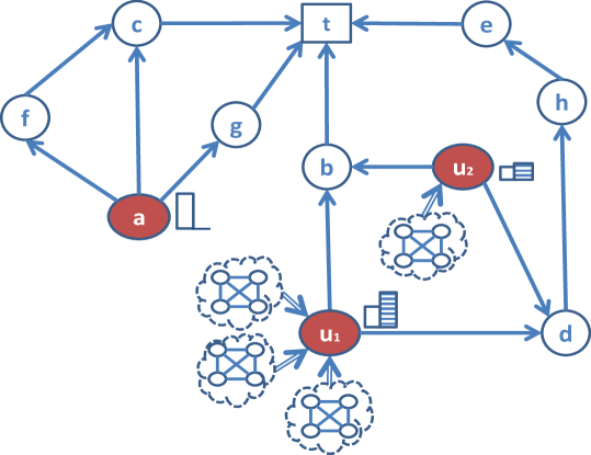
Figure 1: Effect of topological diversity on the outcome of targeted IM.

Two main research questions here arise concerning how to leverage users’ social diversity in order to enhance the performance of a targeted IM task: (R1) how to determine diversity at a large-scale, when we have no a-priori knowledge on user attributes; and (R2) how the seed users should be learned by also considering diversity w.r.t. a target set.

Contributions. In this work we contribute with the definition of a novel problem, named Diversity-sensitive Targeted Influence Maximization (DTIM). To the best of our knowledge, we are the first to bring the concept of topology-driven diversity into targeted IM problems. More specifically, to answer R1, we provide two alternative ways of modeling topology-driven diversity for targeted IM, which depend on the approach adopted to exploit structural information from the diffusion subgraph specific to a given target node. (Loosely speaking, a target-specific diffusion subgraph corresponds the portion of the diffusion graph involved, at a given time step, in the unfolding of the diffusion towards a particular target node.) The first method, dubbed local diversity, is designed to compute node diversity at each step of the expansion of a target-specific diffusion subgraph. The local diversity of a node captures the likelihood of reaching it from nodes outside the currently unfolded target-specific diffusion subgraph. Our second method of topology-driven diversity, dubbed global diversity, exploits the structural information of the fully unfolded target-specific diffusion subgraph, and determines the diversity of nodes that lay on the boundary of the subgraph, i.e., nodes that can receive influence links from nodes external to the subgraph. Intuitively, this would allow us to capture a boundary-spanning effect of external sources of influence coming from the rest of the social graph.

To address question R2, we capitalize on the local diversity and global diversity definitions to develop alternative algorithms for the DTIM problem, dubbed L-DTIM and G-DTIM. Both algorithms follow a greedy approach that exploits the search for shortest paths in the diffusion graph, in a backward fashion from the selected target set.

We evaluate our DTIM methods on a special case of user engagement in OSNs, which concerns the crowd of users who do not actively contribute to the production of social content. Such silent users, a.k.a. lurkers, might have great potential in terms of social capital, i.e., acquired knowledge through the observation of user-generated communications. Therefore, it is highly desirable to encourage (a portion of) silent users to more actively participate and give back to the community. Note that while we previously addressed this problem of user engagement in OSNs via a targeted IM approach in [20, 19], in this work we further delve into understanding such a challenging problem under the new perspective of diversity of the seeds to be identified for maximizing the engagement of silent users.

Experimental evaluation using three real-world OSN datasets was conducted to assess the meaningfulness of our approach, mainly in terms of characteristics of the identified seeds and the activated target users, and how they are affected by tuning the input and model parameters of our methods. We also included comparison with two of the most relevant existing IM methods, namely TIM+ [3] and KB-TIM [21], based on the state-of-the-art RIS approach. While this comparison has highlighted the uniqueness of our methods, it also suggested to improve their efficiency. In this respect, a further important contribution is the revisiting of RIS-based approximation theory to our diversity-sensitive targeted IM problem.

Plan of the paper. The rest of the paper is organized as follows. Section 2 discusses related work, focusing on diversity and targeted IM. Sections 3 presents our diversity-sensitive targeted IM problem, defines two alternative formulations of topology-driven diversity, and presents the L-DTIM and G-DTIM algorithms. In Section 4, we introduce a case study of user engagement for the evaluation of our proposed framework. Experimental evaluation methodology and results are reported in Section 5 and Section 6, respectively. Section 7 describes a RIS-based formulation of DTIM. Section 8 draws conclusions and provides pointers for future research.

2 Related Work

Diversity in information spreading.  Most existing notions of diversity have been developed around structural features of the network, or alternatively based on user profile attributes. This broad categorization applies to various contexts, such as, e.g., web searching and recommendation [22, 23, 24], and information spreading. Focusing on the latter aspect, the authors in [25] propose a measure of controllability, defined as the number of nodes able to spread an opinion through the whole network. In [26], the IC model is extended to take into account the structural diversity of nodes’ neighborhood. Main difference between the above mentioned approaches and our work, relies on the fact that they do not take into account any optimization problem. Other works deal with the problem of estimating the spreading ability of a single node in a network [27, 28]. Node diversity into the IM task has been introduced in [29]. This work shares with ours the linear combination of spread and diversity in the definition of objective function. However, our approach does not depend on user characterization based on topic-biased or categorical distributions.

Targeted influence maximization. Research on targeted IM has gained attention in recent years. A few studies have assumed that the target is unique and a-priori specified. In [30], the authors address the problem of finding the top-$k$ most influential nodes for a specific target user, under the IC model. In [31], the authors investigate optimal propagation policies to influence a target user. In [32], the authors consider the problem of acceptance probability maximization, whereby a selected user (called initiator) wants to send a friendship invitation to a selected target which is not socially close to the initiator (i.e., the two nodes have no common friends). The goal is to find a set of nodes through which the initiator can best approach the target. Unlike the above single-target IM methods, our DTIM approach aims at maximizing the probability of activating a target set which can be arbitrarily large, by discovering a seed set which is neither fixed and singleton nor has constraints related to the topological closeness to a fixed initiator.

In [21], the authors describe a keyword-based targeted IM method, named KB-TIM. This assumes that each user is associated with a weighted term vector to capture her/his preference on advertisements. A user with keywords in common with the advertisement will belong to the target set. KB-TIM relies on a state-of-the-art approach for the classic IM problem, named reverse influence sampling (RIS) [33, 3], which provides theoretical guarantees on the solutions. RIS consists of two main steps: (i) computing, for a fixed number $\theta$ of nodes selected uniformly at random, the reverse reachable sets, i.e., the sets of nodes that can reach them, and (ii) selecting $k$ nodes that cover the maximum number of reverse reachable sets. In [3], the authors show that, when $\theta$ is large enough, this set has high probability of being a near-optimal solution to IM. More in detail, they propose the TIM+ algorithm which derives the parameter $\theta$ as function of a lower bound of the maximum expected spread among all size-$k$ node sets. The steps of KB-TIM are similar to TIM+, but as the former takes into account only users relevant to an advertisement, it defines a different lower bound for $\theta$. Moreover, while in [33, 3] the random reverse reachable sets are sampled online, KB-TIM allows the sampling procedure to be performed offline by building a disk-based reverse reachable index for each keyword. Other targeted IM approaches for target-aware viral marketing purposes are described in [34, 35, 36, 37].

It is worth emphasizing that, except KB-TIM and TIM+, all the above works focus on the IC diffusion model. Note also that the study in [35], which is in principle suited to any diffusion model, actually does not take into account the effect of multiple spreaders (i.e., the diffusion process is considered only for computing the potential influence of each node at a time).

3 Targeted Influence Maximization with Topology-driven Diversity

3.1 Problem statement

Let $\mbox{$\mathcal{G}$}=\mbox{$\mathcal{G}$}_{0}(b,\ell)=\langle\mbox{$\mathcal{V}$},\mbox{$\mathcal{E}$},b,\ell\rangle$ be a directed weighted graph representing the information diffusion graph associated with the social network $\mbox{$\mathcal{G}$}_{0}=\langle\mbox{$\mathcal{V}$},\mbox{$\mathcal{E}$}\rangle$, where $\mathcal{V}$ is the set of nodes, $\mathcal{E}$ is the set of edges, $b:\mbox{$\mathcal{E}$}\rightarrow\mathbb{R}^{*}$ is an edge weighting function, and $\ell:\mbox{$\mathcal{V}$}\rightarrow\mathbb{R}^{*}$ is a node weighting function. The edge weighting function $b$ corresponds to the parameter of the Linear Threshold (LT) model [38, 1], which we adopt as information diffusion model in this work. Under the LT model, each node can be “activated” by its active neighbors if their total influence weight exceeds the threshold associated to that node. More formally, for any edge $(u,v)$, the weight $b(u,v)$ resembles a measure of “influence” produced by $u$ to $v$ and it is such that $\sum_{u\in N^{in}(v)}b(u,v)\leq 1,$ where $N^{in}(v)$ is the in-neighbor set of node $v$. At the beginning of the diffusion process, each node $v$ is assigned a threshold uniformly at random from $\left[0,1\right]$. Given a set $S\subseteq\mbox{$\mathcal{V}$}$ of initial active nodes, an inactive node $v$ becomes influenced or active at time $\tau\geq 1$, if the total weight of its active neighbors is greater than its threshold. The process runs until no more activations are possible. We denote with $\mu(S)$ the final active set, i.e., the set of nodes that are active at the end of the diffusion process starting from $S$.

Given $\mbox{$\mathcal{G}$}=\langle\mbox{$\mathcal{V}$},\mbox{$\mathcal{E}$},b,\ell\rangle$, the node weighting function $\ell$ determines the status of each node as a target, i.e., a node toward which the information diffusion process is directed. More specifically, for any user-specified threshold $L\in[0,1]$, we define the target set $TS$ for $\mathcal{G}$ as:

$$TS=\{v\in\mbox{$\mathcal{V}$}\ |\ \ell(v)\geq L\}.$$ (1)

The objective function of our targeted IM problem is comprised of two functions. The first one, we call capital, is determined as proportional to the cumulative status of the target nodes that are activated by the seed set $S$.

Definition 1 (Capital)

Given $S\subseteq\mbox{$\mathcal{V}$}$, the capital $C(\mu(S))$ associated with the final active set $\mu(S)$ is defined as:

$$C(\mu(S))=\sum\limits_{v\in(\mu(S)\cap TS)\setminus S}\ell(v)$$ (2)

The capital function corresponds to the cumulative amount of the scores associated with the activated (target) nodes, i.e., $C(\mu(S))$. Remarkably, in Eq. (2) we do not consider nodes that belong to the seed set $S$, in order to avoid biasing the seed set by nodes with highest scores.

The second measure is introduced to capture the overall diversity of the nodes in set $S$ w.r.t. the target set. We define it in terms of a function $div_{t}$ that is in turn designed to measure the diversity of a node with respect to each of the target nodes separately.

Definition 2 (Diversity)

Given $S\subseteq\mbox{$\mathcal{V}$}$, the diversity $D(S)$ associated with the target set $TS\subseteq\mbox{$\mathcal{V}$}$ is defined as:

$$D(S)=\sum\limits_{s\in S}\sum_{t\in TS}div_{t}(s)$$ (3)

As previously mentioned, our approach is to measure node diversity in relation to the structural context of the information diffusion graph. In Section 3.2 we shall elaborate on different ways of computing topology-driven diversity, and provide alternative formulations for the $div_{t}$ function.

We now formally define our proposed problem of targeted IM, named Diversity-sensitive Targeted Influence Maximization (DTIM).

Definition 3 (Diversity-sensitive Targeted Influence Maximization)

Given a diffusion graph $\mbox{$\mathcal{G}$}=\langle\mbox{$\mathcal{V}$},\mbox{$\mathcal{E}$},b,\ell\rangle$, a budget $k$, and a threshold $L$, find a seed set $S\subseteq\mbox{$\mathcal{V}$}$ with $|S|\leq k$ of nodes (users) such that, by activating them, we maximize the Diversity-sensitive Capital ($DIC$):

$$\begin{split}S&=\operatornamewithlimits{argmax}\limits_{S^{^{\prime}}\subseteq\mathcal{V}\ s.t.\ |S^{^{\prime}}|\leq k}DIC\\ &=\operatornamewithlimits{argmax}\limits_{S^{^{\prime}}\subseteq\mathcal{V}\ s.t.\ |S^{^{\prime}}|\leq k}\alpha C(\mu(S^{^{\prime}}))+(1-\alpha)D(S^{^{\prime}})\end{split}$$ (4)

where $\alpha\in[0,1]$ is a smoothing parameter that controls the weight of capital $C$ with respect to diversity $D$.

The objective function of the problem in Eq. 4 is defined in terms of linear combination of the two functions, capital and diversity. The problem in Def. 3 preserves the complexity of the IM problem and, as a result, it is computationally intractable, i.e., it is still NP-hard. However, as for the classic IM problem, a greedy solution can be designed since that the natural diminishing property holds for the considered problem, as stated in the following.

Proposition 1

The capital function defined in Eq. (2) is monotone and submodular under the LT model.

Proposition 2

The diversity function defined in Eq. (3) is monotone and submodular.

Proofs of the above propositions can be found in the Appendix. In light of these theoretical results, $DIC$ is also monotone and submodular as it corresponds to a non-negative linear combination of monotone and submodular functions.

In the next section, we conceptualize our notion of user’s topology-driven diversity, which allows us to completely specify the objective function $DIC$ in our DTIM problem.

3.2 Topology-driven Diversity

Our perspective in modeling user diversity is to utilize only structural information given by the topology of a social network graph. Therefore, we take the advantage of a completely unsupervised process to avoid requiring any side-information or a-priori knowledge on user attributes that can enable diversification among users. Instead, we draw inspiration from social science, in that the way a user is connected to others within the OSN (a.k.a. social embeddedness) is recognized as a manifestation of diversity of the individual in that online social environment [16]. This is also strictly related to the theory of boundary spanning [17], which essentially states that OSN users may naturally get knowledge from some of their social contacts and then spread (part of) it to other contacts through one or more components of the social graph (e.g., topically induced communities). Boundary spanning has also been recognized as an important aspect to consider in order to adequately characterize those users that can show different behaviors in terms of information-production and information-consumption when considering them laying on the boundary of graph components [39, 17]. Upon the above intuitions, we start from the following basic assumption:

Principle 1

The diversity of a user in a social graph can be determined based on topological properties of her/his neighborhood.

Definition 4 (Target-specific information diffusion subgraph)

Given the diffusion graph $\mbox{$\mathcal{G}$}=\langle\mbox{$\mathcal{V}$},\mbox{$\mathcal{E}$},b,\ell\rangle$, defined over the social graph $\mbox{$\mathcal{G}$}_{0}=\langle\mbox{$\mathcal{V}$},\mbox{$\mathcal{E}$}\rangle$, a target node $t\in TS$, and a time step $\tau$, we define the target-specific diffusion subgraph as the directed acyclic graph $G_{t}^{(\tau)}=\langle V_{t},E_{t}\rangle\subseteq\mbox{$\mathcal{G}$}_{0}$, rooted in $t$, that corresponds to the portion of $\mathcal{G}$ involved in the unfolding of the diffusion towards $t$, at time $\tau$.

Definition 5 (Boundary set)

Given a target-specific information diffusion subgraph $G_{t}^{(\tau)}$, its boundary set is defined as the set of nodes having at least one incoming connection from nodes in $\mathcal{G}$ outside $G_{t}^{(\tau)}$:

$$B_{t}^{(\tau)}=\{v\in V_{t}\ |\ \exists(u,v)\in\mbox{$\mathcal{E}$}\setminus E_{t}\}$$ (5)

It is worth noticing here that, while the diffusion starts from a set of seed nodes and follows the directed topology of $\mathcal{G}$, a widely adopted way of modeling the search for nodes that could reach target ones is to use the backward or reverse depth-first search (e.g., [2, 33, 3]).

Definition 6 (Expansion of target-specific diffusion subgraph)

Given a target-specific information diffusion subgraph $G_{t}^{(\tau)}$ at time $\tau$, its expansion at time $\tau+1$ is defined as the graph $G_{t}^{(\tau+1)}$ resulting from the reverse unfolding of $G_{t}^{(\tau)}$ such that $G_{t}^{(\tau+1)}$ contains nodes in $\mathcal{G}$ that can reach nodes in the boundary set of $G_{t}^{(\tau)}$. Moreover, a target-specific diffusion subgraph is said fully expanded if no further backward unfolding over $\mathcal{G}$ is possible.

For the sake of simplification, we hereinafter use symbols $G_{t},B_{t}$ instead of $G_{t}^{(\tau)},B_{t}^{(\tau)}$ as the association with a particular time step $\tau$ is assumed to be clear from the context. Moreover, for any $v\in B_{t}$, we denote with $N^{in}_{\neg E_{t}}(v)=N^{in}(v)\setminus\{u\ |\ \exists(u,v)\in E_{t}\}$ the set of in-neighbors of $v$ that are not linked to $v$ in $G_{t}$.

We provide two alternative ways of modeling topology-driven diversity for targeted IM, which depend on the strategy adopted to construct $G_{t}$:

• the first method is designed to compute node diversity at each step of the expansion of the information diffusion subgraph for a given target $t$.Since the method does not require information on the fully expanded diffusion subgraph for $t$, it is referred to as local diversity.

• the second method, named global diversity, is instead designed to compute node diversity on the fully expanded target-specific diffusion subgraph.

In the following, we will provide a complete specification of each of the above introduced diversity methods.

3.2.1 Local Diversity

Our notion of local diversity of node is designed to account for the progressive expansion of the information diffusion graph for a given target node.

Given the currently unfolded $G_{t}$ and a node $v\in B_{t}$ with $N^{in}_{\neg E_{t}}(v)\neq\emptyset$, our goal is to determine the local diversity for every node $u$ in $N^{in}(v)$ based on two main criteria:

Principle 2

The diversity of node $u$ should be proportional to the likelihood of reaching it from nodes outside the currently unfolded target-specific diffusion subgraph $G_{t}$, i.e., proportional to the number of $u$’s in-neighbors in $\mathcal{G}$ not already in $G_{t}$.

Principle 3

The diversity of node $u$ should be proportional to the increment contributed by that node to the number of incoming links not already included in $G_{t}$.

Accordingly, we first characterize the diversity in the boundary set of $G_{t}$, and its incremental update due to the insertion of a new node to $G_{t}$, then we provide our definition of local diversity.

Definition 7 (Boundary diversity of set)

Given the currently unfolded $G_{t}$, the boundary diversity $\delta_{t}$ of $G_{t}$ is defined as the number of nodes in $N_{\neg E_{t}}^{in}(v)$ averaged over nodes $v$ in $B_{t}$:

$$\delta_{t}=\frac{1}{|B_{t}|}\sum_{v\in B_{t}}|N_{\neg E_{t}}^{in}(v)|$$ (6)

Note that the above definition is simple yet convenient to use in incremental computations. Moreover, it is directly related to the amount of possible paths to diffuse towards a particular target node. The study of alternative definitions of boundary diversity could be an interesting direction as future work.

For each $u\in N^{in}(v)$, with $v\in B_{t}$, if $u$ is inserted in $G_{t}$, the boundary diversity will change accordingly, since $B_{t}$ is updated to contain $u$. The boundary diversity w.r.t. $B_{t}$ being updated with $u$, denoted with $\delta^{+u}_{t}$, is straightforwardly determined as follows:

$$\delta^{+u}_{t}=\frac{|B_{t}|\delta_{t}+|N^{in}_{\neg E_{t}}(u)|}{|B_{t}|+1}$$ (7)

Definition 8 (Local diversity)

The local diversity of $u$ is defined as the ratio of the boundary diversity conditional on inclusion of $u$ in $G_{t}$, to the actual boundary diversity:

$$div_{t}(u)=\frac{\delta^{+u}_{t}}{\delta_{t}}=\frac{|B_{t}|}{1+|B_{t}|}\left(1+\frac{|N^{in}_{\neg E_{t}}(u)|}{\sum_{v\in B_{t}}|N^{in}_{\neg E_{t}}(v)|}\right)$$ (8)

Intuitively, the local diversity applies to any node $u$ that is in-neighbor of some node that lays on the boundary of the currently unfolded $G_{t}$, and expresses the increment due to node $u$ to the overall likelihood of being reached from more different portions of the diffusion graph $\mathcal{G}$.

3.2.2 Global Diversity

Our second method of topology-driven diversity computation relies on the availability of structural information of the fully expanded target-specific diffusion subgraph. While this solution loses the advantage of incremental computation, it also opens to the opportunity of using more structural features to measure the diversity of a node.

Given a target node $t$, $G_{t}$ is here meant as the fully expanded diffusion subgraph for $t$. Moreover, the definition of boundary given in Eq. 5 as well as the definition of boundary diversity given in Eq. 6 do not change; however, we will exploit them at a “node level” rather than a “set-level” as for the local diversity.

First, the boundary diversity here assumes a slight different meaning with respect to the local diversity case. It still captures the strength of the flow potentially spanning over portions of the diffusion graph not already unfolded, which makes Principle 2 hold; however, since the target-specific diffusion subgraph $G_{t}$ is considered as definitively unfolded, we conceptualize that:

Principle 4

The boundary spanning should be regarded as exogenous to the diffusion process for a specific target, and hence intuitively associated to external sources of influence coming from the rest of the social graph.

Definition 9 (Boundary diversity of node)

Given a node $v\in B_{t}$, the boundary diversity of $v$ is defined as the contribution of $v$ to the boundary diversity $\delta_{t}$:

$$div_{t}^{B}(v)=\frac{|N^{in}_{\neg E_{t}}(v)|}{|B_{t}|}$$ (9)

Boundary diversity is set to zero for any $v\in V_{t}\setminus B_{t}$.

While the concept of boundary diversity is essential to characterize the connectivity of boundary nodes from outside $G_{t}$, we also consider here to measure their outward connectivity within $G_{t}$ as the contribution a node gives to the average number of out-neighbors of nodes in $B_{t}$ that belong to $G_{t}$. We denote the latter as $|N^{out}_{E_{t}}(v)|/|B_{t}|$. Moreover, we observe that, from the perspective of maximizing diversity of nodes that propagates towards a given target, the overall measure of diversity of node should be not only obviously proportional to its boundary diversity, but also proportional to its outward internal span. The above considerations lead to the following definition.

Definition 10 (Global diversity)

The global diversity of node $v$ is defined as:

$$div_{t}(v)=div_{t}^{B}(v)\times\mathrm{f}\left(\frac{|N^{out}_{E_{t}}(v)|}{|B_{t}|}\right)$$ (10)

where $\mathrm{f}$ is a smoothing function to assign the outward internal span a weight at most equal to the boundary diversity term.

In the following, we will refer to a logarithmic smoothing, i.e., $\mathrm{f}=\log(1+|N^{out}_{E_{t}}(v)|/|B_{t}|)$, since we want the outward internal span of node has an impact lower than the boundary diversity on the overall value of diversity.

3.3 The DTIM algorithms

In this section, we show our algorithmic solutions to the proposed Diversity-sensitive Targeted Influence Maximization problem. According to the local diversity and global diversity criteria previously introduced in Section 3.2, we provide two methods, named L-DTIM and G-DTIM, respectively; due to space limits of this paper, they are concisely reported in Algorithm 1.

Following the lead of the study in [2], L-DTIM and G-DTIM exploit as well the search for shortest paths in the diffusion graph, however in a backward fashion. Along with the information diffusion graph $\mathcal{G}$, the budget integer $k$, the minimum score $L$ and a parameter $\alpha\in\left[0,1\right]$ which controls the balance between capital and diversity, L-DTIM and G-DTIM take in input a real-valued threshold $\eta$. This parameter is used to control the size of the neighborhood within which paths are enumerated: in fact, the majority of influence can be captured by exploring the paths within a relatively small neighborhood; note that for higher $\eta$ values, less paths are explored (i.e., paths are pruned earlier) leading to smaller runtime but with decreased accuracy in spread estimation.

Algorithm 1 DTIM- Diversity-sensitive Targeted Influence Maximization

0: A graph $\mbox{$\mathcal{G}$}=\langle\mbox{$\mathcal{V}$},\mbox{$\mathcal{E}$},b,\ell\rangle$, a budget (seed set size) $k$, a target selection threshold $L\in[0,1]$, a path pruning threshold $\eta\in[0,1]$, a smoothing parameter $\alpha\in[0,1]$.

0: Seed set $S$.

1: $T\leftarrow\mbox{$\mathcal{V}$}$ {nodes that can reach target nodes}

2: for $u\in\mbox{$\mathcal{V}$}$ do

3:    if $\ell(u)\geq L$ then

4:       $TS\leftarrow TS\cup\{u\}$ {identifies the target nodes}

5:    end if

6:    $u.Dset\leftarrow\{\}$ {initializes a data structure that keeps track of node diversity w.r.t. any target}

7: end for

8: while $|S|<k$ do

9:    for $u\in T\setminus S$ do

10:       $u.C,u.D\leftarrow 0$ {initializes each node’s capital and diversity to zero}

11:    end for

12:    $T\leftarrow\emptyset$

13:    for $t\in TS\setminus S$ do

14:       $G_{t}=\langle V_{t},E_{t}\rangle\leftarrow\langle\{t\},\emptyset\rangle$ {initializes DAG rooted in $t$}

15:       ${\textsf{backward}}(\langle t\rangle,1,t)$

16:       if $|S|=0$ then

17:          ${\textsf{updateDiversity}}(t)$

18:       end if

19:    end for

20:    $S\leftarrow S\cup\{bestSeed\}$

21: end while

22: return  $S$

23: procedure ${\textsf{backward}}(\mathcal{P},pp,t)$

24: $v\leftarrow\mathcal{P}.last()$,  $T\leftarrow T\cup\{u\}$

25: while $u\in N^{in}(v)\ \wedge\ u\not\in S\cup\mathcal{P}.nodeSet()$ do

26:    $pp\leftarrow pp\times b(u,v)$ {updates the path probability}

27:    if $pp\geq\eta$ then

28:       $u.C\leftarrow u.C+pp\times\ell(t)$ {updates the overall node capital}

29:       if $|S|=0$ then

30:          $u.inf\leftarrow u.inf+pp$ {increases the overall influence of node $u$ on the current target}

31:          $(^{*})$ $u.Dset(t)\leftarrow div_{t}(u)$ {computes the current node diversity w.r.t. the target by Eq.8}

32:          $G_{t}=\langle V_{t}\cup\{u\},E_{t}\cup\{(u,v)\}\rangle$ {adds the edge $(u,v)$ to the explored DAG}

33:       else

34:          $u.D\leftarrow u.D+pp\times u.Dset(t)$

35:          if $u.DIC>bestSeed.DIC$ then

36:             $bestSeed\leftarrow u$ {sets the current best seed node as $u$}

37:          end if

38:       end if

39:       ${\textsf{backward}}(\mathcal{P}.append(u),pp,t)$

40:    end if

41: end while

42: procedure ${\textsf{updateDiversity}}(t)$

43: for $v\in V_{t}$ do

44:    $(^{**})$ $v.Dset(t)\leftarrow div_{t}(v)$ {computes node diversity w.r.t. the target $t$ by Eq. 10}

45:    $v.D\leftarrow v.D+v.inf\times v.Dset(t)$ {updates the overall node diversity}

46:    $v.inf\leftarrow 0$

47:    if $v.DIC>bestSeed.DIC$ then

48:       $bestSeed\leftarrow v$ {sets the current best seed node as $v$}

49:    end if

50: end for

$(^{*})$ Instruction at line 31 is performed by L-DTIM only.
$(^{**})$ Instruction at line 44 is performed by G-DTIM only.

As previously mentioned, L-DTIM and G-DTIM share the idea of performing a backward visit of the diffusion graph starting from the nodes identified as target (i.e., the nodes $u$ with $\ell(u)\geq L$). To this end, all nodes are initially examined to compute the target set $TS$ (lines 2-5). In order to yield a seed set $S$ of size at most $k$, during each iteration of the main loop (lines 8-21), both the variants of Algorithm 1 compute the set $T$ of nodes that reach the target ones and keep track, into the variable $bestSeed$, of the node with the highest marginal gain (i.e., diversity-sensitive capital $DIC$).

The $bestSeed$ node is found at the end of each iteration upon calling the subroutine backward over all nodes in $TS$ that do not belong to the current seed set $S$. This subroutine takes a path $\mathcal{P}$, its probability $pp$ and the target $t$ from which the visit has started, and extend $\mathcal{P}$ as much as possible (i.e., as long as $pp$ is not lower than $\eta$). Initially, a path is formed by one target node, with probability 1 (line 15). Then, the path is extended by exploring the graph backward, adding to it one, unexplored in-neighbor $u$ at time, in a depth-first fashion. Path probability is updated (line 26) according to the LT-equivalent “live-edge” model [2, 1], and so the capital (line 28). The process is continued until no more nodes can be added to the path.

Both G-DTIM and L-DTIM compute the node diversity only at the first iteration of the main loop, i.e., when the seed set $S$ is empty. Indeed, for each node, we keep track of its diversity w.r.t. each target it can reach, by using data structure $Dset$. A major difference between the two variants is that in G-DTIM the node diversity is computed (through the subroutine updateDiversity) only when the whole subgraph rooted in $t$ has been completely built (line 44). In L-DTIM, instead, the node diversity is updated every time the node has been reached (line 31). Note that the instruction at line 31 (resp. 44) is performed by L-DTIM (resp. G-DTIM) only. The value of diversity of a node $v$ is, in both the variants, smoothed with the influence that $v$ might exert on $t$, contributing to the overall diversity $D$ of $v$ (line 45).

Note that both the numerical values yielded by both global diversity and local diversity functions $div_{t}$ might be subject to scaling in order to enable a fair comparison with the numerical value yielded by the capital.

Example 2. Consider the example in Fig. 2, where the target set includes the square border node $\{t\}$. Let’s assume for simplicity we set $k=1$, $\alpha=0.5$, $\eta=0$ and we ignore the spread computation for nodes inside the other components of $G_{t}$ (represented within clouds in the figure). Moreover, the double arrows connecting these components to nodes $u_{1}$ and $u_{2}$ count as two edges each. In the following, we denote with $pp\left[x\rightarrow\cdots\rightarrow y\right]$ the probability of the path from $x$ to $y$, and with $x.inf$ the overall influence exerted by node $x$ to the target.

The target node $t$ can be reached through $a$ (with $a.inf=pp\left[a\rightarrow f\rightarrow c\rightarrow t\right]+pp\left[a\rightarrow c\rightarrow t\right]+pp\left[a\rightarrow g\rightarrow t\right]=0.098+0.06+0.24$), $b$ (with $b.inf=pp\left[b\rightarrow t\right]=0.35$), $c$ (with $c.inf=pp\left[c\rightarrow t\right]=0.2$), $d$ (with $d.inf=pp\left[d\rightarrow h\rightarrow e\rightarrow t\right]=0.045$), $e$ (with $e.inf=pp\left[e\rightarrow t\right]=0.15$), $f$ (with $f.inf=pp\left[f\rightarrow c\rightarrow t\right]=0.14$), $g$ (with $g.inf=pp\left[g\rightarrow t\right]=0.3$), $h$ (with $h.inf=pp\left[h\rightarrow e\rightarrow t\right]=0.09$), $u_{1}$ (with $u_{1}.inf=pp\left[u_{1}\rightarrow d\rightarrow h\rightarrow e\rightarrow t\right]+pp\left[u_{1}\rightarrow b\rightarrow t\right]=0.0135+0.21$), and $u_{2}$ (with $u_{2}.inf=pp\left[u_{2}\rightarrow d\rightarrow h\rightarrow e\rightarrow t\right]+pp\left[u_{2}\rightarrow b\rightarrow t\right]=0.0315+0.14$). Node $a$ has the largest chance of success in activating $t$, which results in the highest capital $C$. However, since $a$ does not have in-neighbors, its diversity is equal to zero for both the diversity formulations.

Let us first focus on the behavior of G-DTIM. According to Eq. 5, the set of boundary nodes is $B_{t}=\{u_{1},u_{2}\}$. By definition of global diversity (Eq. 10), G-DTIM computes the following values: $u_{1}.D=2.08$ (as $div_{t}^{B}(u_{1})=6/2$ and $div_{t}(u_{1})=3\times\log(1+2/2)$), $u_{2}.D=0.69$ (as $div_{t}^{B}(u_{2})=2/2$ and $div_{t}(u_{1})=1\times\log(1+2/2)$). By applying the max-normalization to the node diversity, the final values are $u_{1}.D=1$ and $u_{2}.D=0.33$. As a result, for G-DTIM node $u_{1}$ is chosen as seed node since it has diversity-sensitive capital ($DIC=0.22\times 0.5\times(0.5+1)=0.165$) higher than that of $a$ ($DIC=0.4\times 0.5\times(0.5+0)=0.1$) and $u_{2}$ ($DIC=0.13\times 0.5\times(0.5+0.33)=0.05$).

The values of node diversity computed by L-DTIM depend on the order in which nodes are reached during the backward visit. Assume to visit first the branch starting from node $e$. According to Eq. 8, L-DTIM computes the following values of node diversity: $e.D=0.625$ ($div_{t}(e)=1/2\times(1+1/4)$ as $B_{t}=\{t\}$), $h.D=0.83$ ($div_{t}(h)=2/3\times(1+1/4)$ as $B_{t}=\{t,e\}$), $d.D=1$ ($div_{t}(d)=2/3\times(1+2/4)$ as $B_{t}=\{t,h\}$), and, assuming to visit $u_{1}$ before $u_{2}$, $u_{1}.D=1.47$ ($div_{t}(u_{1})=2/3\times(1+6/5)$ as $B_{t}=\{t,d\}$), $u_{2}.D=0.9$ ($div_{t}(u_{2})=3/4\times(1+2/10)$ as $B_{t}=\{t,d,u_{1}\}$). Analogously, it proceeds in computing the node diversity through branches $c$ and $g$, whose values of diversity are lower than $0.9$ (not reported for the sake of readability). L-DTIM eventually computes the following diversity: $b.D=0.92$ ($div_{t}(b)=3/4\times(1+2/9)$ as $B_{t}=\{t,u_{1},u_{2}\}$), $u_{1}.D=1.2$ ($div_{t}(u_{1})=3/4\times(1+6/10)$ as $B_{t}=\{b,u_{1},u_{2}\}$), and $u_{2}.D=0.92$ ($div_{t}(u_{2})=3/4\times(1+2/9)$ as $B_{t}=\{b,u_{1},u_{2}\}$). Upon max-normalization to the values so obtained, L-DTIM will choose $b$ as seed node since it has diversity-sensitive capital ($DIC=0.35\times 0.5\times(0.5+0.77)=0.22$) higher than that of $u_{1}$ ($DIC=0.22\times 0.5\times(0.5+1)=0.165$).

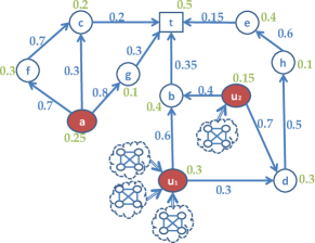
Figure 2: Targeted IM vs. diversity-sensitive targeted IM. Edge weights (values in blue) and node weights (values in green) are computed by functions $b$ and $\ell$. To avoid cluttering of the figure, the node activation thresholds used by LT model here coincide with the node weights.

4 Using DTIM to engage silent users in social networks

We evaluate our framework of targeted IM with topology-driven diversity on a special case of user engagement in OSNs, which refers to the problem of how to turn silent users into more active contributors in the community life.

All large-scale OSNs are characterized by a participation inequality principle: the crowd does not take an active role in the interaction with other members, rather it takes on a silent role. Silent users are also referred to as lurkers, since they gain benefit from information produced by others, by observing the user-generated communications at all stages (e.g., reading posts, watching videos, etc.), but without significantly giving back to the community [40, 15].

Social science and human-computer interaction research communities have widely investigated the main causes that explain lurking behaviors, which include subjective reticence (rather than malicious motivations) to contribute to the community wisdom, or a feeling that gathering information by browsing is enough without the need of being further involved in the community. Moreover, lurking can be expected or even encouraged because it allows users (especially newcomers) to learn or improve their understanding of the etiquette of an online community [40].

Regardless of their motivations, lurkers might have great potential in terms of social capital, because they acquire knowledge from the OSN. They can become aware of the existence of different perspectives and may make use of these perspectives in order to form their own opinions, but they are unlikely to let other people know their value. In this regard, it might be desirable to engage such users, or delurk them, i.e., to develop a mix of strategies aimed at encouraging lurkers to return their acquired social capital, through a more active participation to the community life.

Engagement actions towards silent users can be categorized into four types [15]: reward-based external stimuli, providing encouragement information, improvement of the usability and learnability of the system, guidance from elders/master users to help lurkers become familiar with the system as quickly as possible. It is worth emphasizing that our approach is independent on the particular strategy of delurking being adopted. The goal here is how to instantiate our DTIM algorithms in a user engagement scenario where lurkers are regarded as the target users of the diffusion process. Therefore, our goal becomes: Given a budget $k$, to find a set of $k$ nodes that are capable of maximizing the diversity-sensitive capital, i.e., the likelihood of activating the target silent users through diverse seed users.

A key aspect of our approach in this scenario is that the selection of target users is based on the solution produced by a lurker ranking algorithm [41, 39, 42] applied to the social network graph $\mbox{$\mathcal{G}$}_{0}$. In Section 4.1 we provide a summary of the lurker ranking method we used in this work, and in Section 4.2 we describe how the input diffusion graph for DTIM is modeled, following our early work in [20].

4.1 Identifying target users through LurkerRank

Lurker ranking methods, originally proposed in [41, 39], are designed to mine silent user behaviors in the network, and hence to associate users with a score indicating her/his lurking status. Lurker ranking methods rely upon a topology-driven definition of lurking which is based on the network structure only. Upon the assumption that lurking behaviors build on the amount of information a node receives, the key intuition is that the strength of a user’s lurking status can be determined based on three basic principles: overconsumption, authoritativeness of the information received, non-authoritativeness of the information produced.

The above principles form the basis for three ranking models that differently account for the contributions of a node’s in-neighborhood and out-neighborhood. A complete specification of the lurker ranking models is provided in terms of PageRank and AlphaCentrality based formulations. For the sake of brevity here, we will refer to only one of the formulations described in [41, 39], which is that based on the full in-out-neighbors-driven lurker ranking, hereinafter dubbed simply as LurkerRank (LR).

Given the directed social graph $\mbox{$\mathcal{G}$}_{0}=\langle\mbox{$\mathcal{V}$},\mbox{$\mathcal{E}$}\rangle$, where any edge $(u,v)$ means that $v$ is is “consuming” or “receiving” information from $u$, the LurkerRank $LR(v)$ score of node $v$ is defined as:

$$LR(v)=\mbox{$d$}[\mathcal{L}_{\mathrm{in}}(v)\ (1+\mathcal{L}_{\mathrm{out}}(v))]+(1-\mbox{$d$})p(v)$$ (11)

where $\mathcal{L}_{\mathrm{in}}(v)$ is the in-neighbors-driven lurking function:

$$\mathcal{L}_{\mathrm{in}}(v)=\frac{1}{out(v)}\sum_{u\in N^{in}(v)}\frac{out(u)}{in(u)}LR(u)$$ (12)

and $\mathcal{L}_{\mathrm{out}}(v)$ is the out-neighbors-driven lurking function:

$$\mathcal{L}_{\mathrm{out}}(v)=\frac{in(v)}{\sum_{u\in N^{out}(v)}in(u)}\sum_{u\in N^{out}(v)}\frac{in(u)}{out(u)}LR(u)$$ (13)

where: $in(v)$ (resp. $out(v)$) denotes the size of the set of in-neighbors (resp. out-neighbors) of $v$, $d$ is a damping factor ranging within [0,1] (usually set to 0.85), and $p(v)$ is the value of the personalization vector, which is set to $1/|\mbox{$\mathcal{V}$}|$ by default. To prevent zero or infinite ratios, the values of $in(\cdot)$ and $out(\cdot)$ are Laplace add-one smoothed.

4.2 Modeling the diffusion graph

In Section 3.1, we introduced symbol $\ell(v)$ to denote the weight of node $v$ that quantifies its status as target. In this application scenario, the higher is the lurker ranking score of $v$ the higher should be $\ell(v)$.

We define the node weighting function $\ell$ upon scaling and normalizing the stationary distribution produced by the LurkerRank algorithm over $\mbox{$\mathcal{G}$}_{0}$. The scaling compensates for the fact that the lurking scores produced by LurkerRank, although distributed over a significantly wide range (as reported in [39]), might be numerically very low (e.g., order of $1.0e\mbox{-}3$ or below). Moreover, we introduce a small smoothing constant in order to avoid that the highest lurking scores are mapped exactly to 1. Formally, for each node $v\in\mbox{$\mathcal{V}$}$, we define the node lurking value $\ell(v)\in[0,1)$ as follows:

$$\ell(v)=\frac{\widetilde{\pi_{v}}-min_{r}}{(max_{r}-min_{r})+\epsilon_{r}}$$ (14)

where $\widetilde{\pi}$ denotes the stationary distribution of the lurker ranking scores ($\pi$) divided by the base-10 power of the order of magnitude of the minimum value in $\pi$, $\widetilde{\pi_{v}}$ is the value of $\widetilde{\pi}$ corresponding to node $v$, $max_{r}=\max_{u\in\mbox{$\mathcal{V}$}}\widetilde{\pi_{u}}$, $min_{r}=\min_{u\in\mbox{$\mathcal{V}$}}\widetilde{\pi_{u}}$, and $\epsilon_{r}$ is a smoothing constant proportional to the order of magnitude of the $max_{r}$ value.

In order to define the edge weights so that they express a notion of strength of influence from a node to another (as normally required in an information diffusion model), we again exploit information derived from the ranking solution obtained by LurkerRank as well as from the structural properties of the social graph. Our key idea is to calculate the weight on edge $(u,v)\in\mbox{$\mathcal{E}$}$ proportionally to the fraction of the original lurking score of $v$ given by its in-neighbor $u$:

$$b_{0}(u,v)=\left[\sum_{w\in N^{in}(v)}\frac{out(w)}{in(w)}\pi_{w}\right]^{-1}\frac{out(u)}{in(u)}\pi_{u}$$ (15)

Using Eq. (15), we finally define the edge weight as:

$$b(u,v)=b_{0}(u,v)\times e^{\ell(v)-1}$$ (16)

Note that Eq. (16) meets the requirement $\sum_{u\in N^{in}(v)}b(u,v)\leq 1$, and accounts for $\ell(v)$ such that the resulting weight on $(u,v)$ is lowered for higher $\ell(v)$, i.e., the more a node acts as a lurker, the more active in-neighbors are needed to activate that node.

5 Evaluation methodology

5.1 DTIM settings

We experimentally varied the input and model parameters in DTIM methods, namely: the size of seed set ($k$), the target selection threshold ($L$), the path pruning threshold ($\eta$), and the parameter $\alpha$ to control the contribution of diversity versus capital in the objective function of DTIM methods. Note that, to simplify the interpretation of $L$, we will instead use symbol $L\textit{-perc}$ to denote a percentage value that determines the setting of $L$ such that the selected target set corresponds to the top-$L\textit{-perc}$ of the distribution of scores yielded by function $\ell$; particularly, we set $L\textit{-perc}\in\{5\%,10\%,25\%\}$. As concerns $\eta$, though $\eta=1.0e\mbox{-}03$ is the default as used in other IM algorithms (e.g.,[2]), we set it to a lower value, $\eta=1.0e\mbox{-}04$, to impact even less on the unfolding of the information diffusion process; moreover, we will not present results corresponding to $\eta=0$ (i.e., no path-pruning), since we observed this negatively affects the runtime by several orders of magnitude while yielding nearly identical results to those corresponding to $\eta=1.0e\mbox{-}04$.

5.2 Competing methods

We considered comparison with TIM+ [3] and KB-TIM [21], which are state-of-the-art solutions to the IM (resp. targeted IM) problem, based on the RIS approach (cf. Sect. 2).

Comparing DTIM with a non-targeted IM algorithm like TIM+ required to evaluate the quality of seed sets produced by the competing algorithm under a targeted scenario. To this purpose, we simply let TIM+ compute a size-$k$ seed set over the entire graph and then we estimated the capital over different target sets in accord with the setting of DTIM. We considered two opposite settings for the main parameter ($\epsilon$) in TIM+: (i) the default $\epsilon=0.1$, which provides strong theoretical guarantees yet is adversarial to the algorithm’s memory consumption, and (ii) $\epsilon=1.0$, which conversely provides no approximation guarantees but high empirical efficiency; note that the latter setting was also used by the TIM+’s authors in [3] for the comparison with SimPath. We used default settings for the other parameters in TIM+.

As concerns KB-TIM, we modified the keyword-based target selection stage to make it equivalent to the target selection adopted in DTIM. KB-TIM requires two main input files to drive the target selection: (i) a sort of document-term sparse matrix, such that each node (document) in the graph is assigned a list of $keyword,\#occurrences$ pairs, and (ii) a list of keyword-queries, so that each query corresponds to the selection of a subset of nodes in the graph. To prepare these input files, we defined three queries corresponding to the setting $L\textit{-perc}\in\{5\%,10\%,25\%\}$, and accordingly created the sparse matrix so that each node was assigned a keyword for each of the top-ranked subsets it belongs to (e.g., a node in the top-10% set of lurkers will be assigned two keywords, as it is also in the top-25% set); moreover, the $\#occurrences$ associated with any keyword for a given node $v$ was calculated as the node lurking value $\ell(v)$ suitably scaled and truncated to its integer part. Also, we used the incremental reverse-reachable index ($IRR$) in KB-TIM.

5.3 Data

We used FriendFeed [43], GooglePlus [44], and Instagram [42] network datasets. Note that, for the sake of significance of the information diffusion process in latter network, we selected the induced subgraph corresponding to the maximal strongly connected component of the original network graph, hereinafter referred to as Instagram-LCC (LCC stands for largest connected component). As major motivations underlying our data selection, we wanted to maintain continuity with our previous studies [39, 42] and use publicly available datasets. Table I summarizes main structural characteristics of the evaluation network datasets.

data	# nodes	# links	avg	avg	clust.	assorta-
			in-deg.	path len.	coeff.	tivity
FriendFeed	​​493,019​​	​​19,153,367​​	38.85	3.82	0.029	-0.128
GooglePlus	​​107,612​​	​​13,673,251​​	127.06	3.32	0.154	-0.074
Instagram-LCC​​​	17,521	617,560	35.25	4.24	0.089	-0.012

TABLE I: Summary of the evaluation network datasets

6 Results

We present results of the evaluation of our proposed DTIM algorithms according to three main objectives: analysis of the identified seed nodes (Sect. 6.1), analysis of the activated target nodes (Sect. 6.2) and efficiency analysis (Sect. 6.3).

6.1 Evaluation of identified seed nodes

6.1.1 Seed set overlap

In order to investigate the impact of taking into account diversity on the seed identification process, we initially analyzed the matching among seed sets produced by the two DTIM methods with varying $\alpha$.

This analysis of seed sets was twofold: (i) pair-wise evaluation of the overlaps between seed sets produced by a particular DTIM method by varying $\alpha$, and (ii) pair-wise evaluation of the overlaps between seed sets produced by G-DTIM and L-DTIM for particular values of $\alpha$. Unless otherwise specified, results correspond to the largest sizes of target set and seed set we considered (i.e., $L\textit{-perc}=25\%$ and $k=50$), and express the normalized overlap of any two seed sets, i.e., their intersection divided by the seed set size.

Normalized seed set overlap.  On GooglePlus (Fig. 3), the normalized overlap values span over the full range $[0.0,1.0]$, for both methods. In the heatmap corresponding to G-DTIM, an overlap above than $50\%$ is observed for values of $\alpha$ in different subintervals, while variations in the seed set are generally more uniform for L-DTIM, whereby the normalized overlap increases for higher values of $\alpha$. Also, for both methods there is no overlap when comparing the seed set obtained for $\alpha=0$ (i.e., full contribution of diversity in the DTIM objective function) with the seed set obtained for any $\alpha>0$. These remarks generally hold regardless of the target set size when using L-DTIM, while the contingencies of null overlap are more likely to occur for lower $L\textit{-perc}$ when using G-DTIM. A large spectrum of normalized overlap values are observed on FriendFeed as well (results not shown), particularly at least $0.25$ for G-DTIM and $0.4$ for L-DTIM. Null overlap is mainly observed for low seed set size ($k=5$ using L-DTIM, and $k\leq 15$ using G-DTIM). By contrast, Instagram-LCC generally shows a quite higher overlap than in the other networks (results not reported), which might be ascribed to the particular contingency of strong connectivity that characterizes Instagram-LCC.

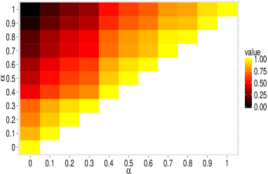
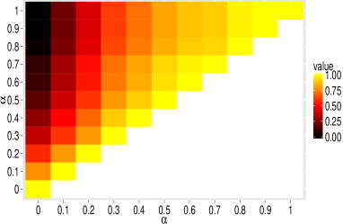
(a) G-DTIM	(b) L-DTIM

Figure 3: Heatmaps of normalized overlap of seed sets, for varying $\alpha$, with $L\textit{-perc}=25\%$ and $k=50$, on GooglePlus.

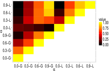
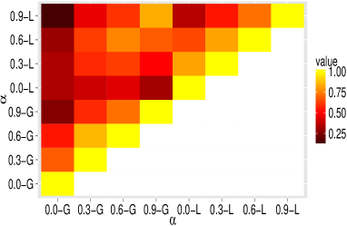
(a) GooglePlus	(b) FriendFeed

Figure 4: Heatmaps of normalized overlap of seed sets between G-DTIM and L-DTIM, for $\alpha=\{0.0,0.3,0.6,0.9\}$, $L\textit{-perc}=25\%$ and $k=50$. (Suffix -L, resp. -G, denotes a particular setting of $\alpha$ that refers to L-DTIM, resp. G-DTIM.)

Comparison between G-DTIM and L-DTIM seed sets.  Figure 4 shows results on the comparison of seed sets identified by G-DTIM and L-DTIM, respectively, corresponding to $\alpha=\{0.0,0.3,0.6,0.9\}$. On GooglePlus (Fig. 4(a)), the seed sets appear to be significantly different from each other for higher contributions of diversity in the objective function ($\alpha<0.3$), while values of normalized overlap in the range $[0.5,1]$ are observed for higher values of $\alpha$. Analogous observations can be drawn for FriendFeed (Fig. 4(b)), yet with lower overlap values also for values of $\alpha$ in the range $[0.6,0.9]$ (i.e., normalized overlap around $0.75$).

Comparison with TIM+ and KB-TIM.  We also analyzed the matching between seed sets produced by DTIM algorithms and competing ones (results not shown). Here we refer to the setting $\alpha=1.0$ (i.e., no diversity contribution), since TIM+ and KB-TIM do not integrate any diversity notion in their formulations. The minimum overlap of seed sets produced by DTIM is reached against KB-TIM in all cases and on all datasets; in particular, with the setting $k=50,L\textit{-perc}=25\%$, 0.48 for FriendFeed, 0.46 for GooglePlus, 0.60 for Instagram-LCC. In general, for large $k$, the normalized overlap is within medium regimes, while it is close or equal to zero on FriendFeed. Only for $k=5$, the normalized overlap corresponds to mid-high values on GooglePlus and Instagram-LCC. DTIM with $\alpha=1$ can have relatively high overlap with TIM+ (about 0.75), especially for high $L\textit{-perc}$, on all datasets. However, for lower $L\textit{-perc}$, the overlap is low (for smaller $k$) to medium (for higher $k$).

Discussion.  The seed set overlap analysis has revealed that accounting for diversity can yield significant differences in the behavior of the DTIM methods in terms of seed identification. Indeed, by varying $\alpha$ within its full regime of values leads to a wide spectrum of values of normalized seed set overlap. In particular, the changes in overlap are more evident when varying $\alpha$ at lower regimes, thus indicating that higher contribution of diversity w.r.t. capital leads to more significantly diversified seed sets. Remarkably, the overlap can be close to zero when comparing two seed sets respectively obtained with $\alpha=0$ and with $\alpha=1$, i.e., completely different seed nodes can be identified when accounting for either diversity or capital only in the target IM objective function.

The two proposed notions of diversity turn out to be quite dissimilar to each other: indeed, the normalized overlap of seed sets yielded by L-DTIM and G-DTIM, respectively, is generally below 50%, which is further reduced for low values of $\alpha$. The local diversity notion appears to be less sensitive to $\alpha$ than global diversity; however, for low $\alpha$ and size of target set, L-DTIM tends to produce more diverse seed sets than G-DTIM, for any particular setting of $k$.

Our DTIM methods with $\alpha=1$ produce seed sets that have overlap with KB-TIM ones below $50\%$ on FriendFeed and GooglePlus, and $60\%$ on Instagram for $k=50$, $L\textit{-perc}=25\%$; when compared to TIM+, the seed set overlap can be relatively higher.

6.1.2 Structural characteristics of seeds

We analyzed topological characteristics of the identified seeds, focusing on basic measures of node centrality, namely outdegree, betweenness, and coreness. Due to space limits, we present here a summary of main findings, and refer the reader to the Appendix for detailed results.

One major remark that stands out is that accounting for diversity in DTIM methods produces the effect of choosing seed nodes that can differ from those that would be obtained otherwise (i.e., using only capital term in the objective function) according to selected topological criteria. This result, coupled with analogous considerations previously drawn about diversification in terms of set overlap, hence strengthens the significance of accounting for diversity in the targeted IM process. Structural characteristics tend to be marginally affected by the setting of $L\textit{-perc}$ when L-DTIM is used, while the behavior with G-DTIM is much more dependent on $L\textit{-perc}$, especially for smaller size of target set ($L\textit{-perc}=5\%$). Also, each of the competing methods leads to the identification of seeds that are less different from each other than DTIM seeds being obtained for most of the settings of $\alpha$, in terms of all the topological measures considered.

6.2 Evaluation of activated target nodes

6.2.1 Capital

We discuss results on the expected capital of the target users activated by a given set of seed users. The estimation procedure is based on the results of $I_{MC}$ Monte Carlo simulations of the LT diffusion process, with $I_{MC}$ set to 10 000. Note that while the identification of the seeds depends on the full DTIM objective function, here we focus on the value of the capital function $C$ only.

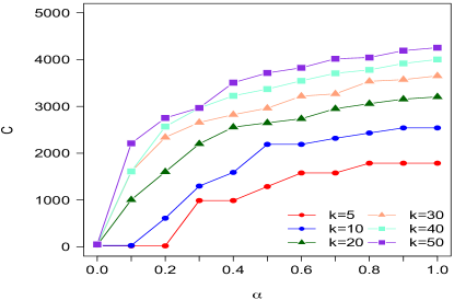
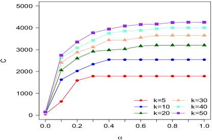
(a) G-DTIM	(b) L-DTIM

Figure 5: Capital in function of $\alpha$ and $k$, with $L\textit{-perc}$ set to 25%, on GooglePlus.

Beyond the expected increase in capital with $\alpha$ (which means weighting less diversity than capital in the objective function), the impact of $\alpha$ on the behavior of DTIM algorithms is evident, especially for $k>10$, with capital value that can vary up to three orders of magnitude. The generally upward trends of $C$ are explained in function of both $\alpha$ and $k$, particularly they are more rapidly increasing for mid-low $\alpha$ and $k>10$. Also on all datasets, L-DTIM yields a higher average capital value, for every $k$, than that observed with G-DTIM. Similar overall behaviors are shown by the DTIM algorithms for different sizes of target set.

More in detail, on GooglePlus (Fig. 5), when using G-DTIM the capital value increases rapidly, reaching around $80\%$ for $\alpha<0.5$ and $k\geq 20$; for L-DTIM, we observe an even sharper increase in the value of $C$ for small $\alpha$ (0.2), then the trends become nearly constant for higher $\alpha$. Similar behaviors are shown on FriendFeed, though the increasing trends are less monotone for $k<30$. On Instagram-LCC, the relatively small size and high connectivity of this network makes capital values subject to an average variation of about $15\%$ over the full range of $\alpha$.

Comparison with TIM+ and KB-TIM.  Capital obtained by DTIM methods is shown to be much higher than that of competing methods, on all networks and for various $k$ and $L\textit{-perc}$. The performance gain is more significant on FriendFeed, with average percentage of increment from $9.85\%$ (for $L\textit{-perc}=5\%$) to $3.49\%$ ($L\textit{-perc}=25\%$) w.r.t. TIM+, and even larger (from $35\%$ to $59\%$) w.r.t. KB-TIM. On the two largest networks, as the size of target set increases, a general decreasing trend is observed in the gap between DTIM and TIM+ (resp. KB-TIM) capital values, which might be explained since a larger target set implies that a larger fraction of the entire node set could be reached.

6.2.2 Target activation probabilities

A further stage of evaluation was performed to understand how different settings of $\alpha$ and $k$ impact on the activation probability of nodes targeted by DTIM methods. We regard the activation probability of a node as the number of times it has been activated divided by the number of runs of Monte Carlo simulation for the estimation of capital. Due to space limits, we present here a summary of main findings concerning this evaluation, and refer the reader to the Appendix for detailed results.

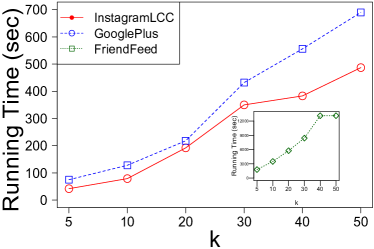
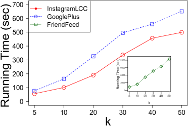
(a) G-DTIM	(b) L-DTIM

Figure 6: Time performance (in seconds) for varying $k$, with $\alpha=0.5$ and $L\textit{-perc}=25\%$.

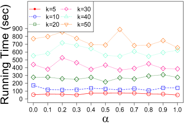
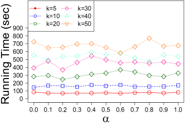
(a) G-DTIM	(b) L-DTIM

Figure 7: Time performance (in seconds) for varying $k$ and $\alpha$, with $L\textit{-perc}=25\%$, on GooglePlus.

For both DTIM algorithms, the activation probability follows a non-decreasing trend as $\alpha$ increases. The likelihood of obtaining high activation probability grows with $\alpha$, i.e., the amount of target nodes that have high probability of activation increases by increasing $\alpha$. The analysis of density distributions also puts in evidence that the density peak corresponding to low activation probability is higher for lower values of $\alpha$, whereas the density corresponding to high activation probability increases for higher values of $\alpha$. Nevertheless, on the two largest datasets, we also observe that choosing a relatively large $k$ leads a significant portion of target nodes to have mid-high activation probabilities already for $\alpha=0.1$, thus suggesting that target nodes can be activated even with strongly unbalancing capital with diversity. By contrast, when choosing a small $k$, little changes in the value of $\alpha$ can significantly impact on the amount of more likely activated target nodes.

6.3 Efficiency analysis

Figure 6 reports on time performance of G-DTIM and L-DTIM on the various networks, for $5\leq k\leq 50$ and $\alpha=0.5$. The execution time of both methods shows a roughly linear increase with $k$, on all networks. (Note that the FriendFeed time series are shown in the figure insets, as they correspond to orders of magnitude higher than for the other networks, due to the larger size of FriendFeed). Also, G-DTIM turns out to be slightly faster than L-DTIM, which might be ascribed to the fewer computations of node diversity needed by G-DTIM w.r.t. L-DTIM.

As shown in Fig. 7 for GooglePlus in particular (though similar behaviors also characterize the other networks), varying $\alpha$ with fixed $k$ does not significantly impact on the time performance of both DTIM methods. This would indicate that, for a given seed set size, the methods’ effort in computing the global/local diversity as well as the capital contributions in the objective function is not greatly affected by the value of $\alpha$. Analogous remarks are also drawn for the other settings of $L\textit{-perc}$.

As regards TIM+ and KB-TIM (results not shown), it comes without surprise that both outperform DTIM methods. For instance, on our largest network (i.e., FriendFeed), the execution times of TIM+ (with $\epsilon=0.1$) are between $6.3$ ($k=50$) and $11.9$ ($k=5$) seconds — note that the increase in runtime by decreasing $k$ is in line with the theoretical and experimental results shown in [3]; yet, KB-TIM execution times are always below 0.7 seconds regardless of $L\textit{-perc}$, which might also depend on the extremely low number of queries and keywords used by KB-TIM in our setting.

7 RIS-based formulation of DTIM

The gap in efficiency shown by our DTIM algorithms w.r.t. the competing RIS-based ones, prompted us to investigate how to adapt RIS-based approximations to our diversity-sensitive, targeted IM problem.

7.1 Revisiting RIS theory for the DTIM problem

The reverse influence sampling (RIS) [33] relies on the concept of reverse reachable (RR) set. Intuitively, the random RR set generated from $\mathcal{G}$ for a randomly selected user $u$ (i.e., the root of the RR set) contains the users who could influence $u$. By generating many random RR sets on different random users, if a user has high potential to influence other users, then s/he will likey appear in those random RR sets. Thus, if a seed set covers most of the RR sets, it will likely maximize the expected spread. Upon this principle, Corollary 1 in [3] states that $\mathbb{E}[F(S)/\theta]=\mathbb{E}[\mu(S)]/n$, where $F(S)$ denotes the number of RR sets covered by the node set $S$, $\mu(S)$ is the spread of $S$, $\theta$ is the number of RR-sets, and $n=|\mbox{$\mathcal{V}$}|$.

In our setting, every node $v\in\mbox{$\mathcal{V}$}$ is selected as root of an RR-set with probability proportional to its status as target node, i.e., $p(v)=\frac{\ell^{\prime}(v)}{L_{TS}}$, where $\ell^{\prime}(v)=\ell(v)$ if $v\in TS$, zero otherwise, and $L_{TS}=\sum_{v\in TS}\ell^{\prime}(v)$. In the following, we state that for any set of nodes $S$, the expected value of the fraction of RR sets covered by $S$ is equal to the normalized expected value of the capital associated with the activation of target nodes due to $S$ as seed set.

Proposition 3

$$\mathbb{E}\left[\frac{F(S)}{\theta}\right]=\frac{\mathbb{E}[C(\mu(S))]}{L_{TS}}$$ (17)

The proofs of all propositions in this section are reported in the Appendix.

Estimation of the number of RR sets.  In [3], the objective is to find a number $\theta$ of RR sets such that $\theta\geq\lambda/OPT$, where $OPT$ denotes the maximum expected spread of any size-$k$ seed set, and $\lambda$ is determined as a function of the size of the graph, $k$ and the approximation factor $\epsilon$. Since $OPT$ is unknown, a lower bound for it must be computed.

Following from Lemma 4 in [3], the expected spread of a randomly sampled node can be expressed in terms of the expected value $EPT$ of the number of edges pointing to nodes in an RR set (width), such that $EPT\leq\frac{m}{n}OPT$ holds, with $m=|\mbox{$\mathcal{E}$}|$. We revise this result to state that the expected value of the width of an RR set can be an accurate estimator of the capital associated with any node when randomly selected as a seed.

Proposition 4

$$(L_{TS}/m)\ EPT=\mathbb{E}[C(\{v\})]\ \leq\ OPT$$ (18)

To avoid unnecessarily large values of $\theta$, it is desired to find a lower error bound in terms of the mean of the expected spread of a set $S$ (over the randomness in $S$ and the influence propagation process), denoted as $KPT$, such that $(n/m)EPT\leq KPT\leq OPT$ holds. To this aim, Lemma 5 in [3] estimates $KPT$ as $KPT=n\mathbb{E}_{R\sim\mathcal{R}}[\kappa(R)]$, taking the average over a set of random RR sets $R$ from the possible world $\mathcal{R}$, where $\kappa(R)=1-(1-\frac{w(R)}{m})^{k}$ and $w(R)$ is the width of $R$. Again, we revise this result in our setting:

Proposition 5

Given a random RR set $R$, and denoted with $TS_{R}$ the set of target nodes in $R$, it holds that

$$\widehat{\kappa}(R)=\left[1-\left(1-\frac{|TS_{R}|}{m}\right)^{k}\right]\frac{\sum_{v\in R}\ell^{\prime}(v)}{|TS_{R}|}.$$ (19)

Therefore,

$$KPT=n\mathbb{E}_{R\sim\mathcal{R}}[\widehat{\kappa}(R)].$$ (20)

7.2 Developing RIS-based DTIM algorithms

We sketch here a reformulation of DTIM based on the RIS approach. To this purpose, we start from TIM+ and adapt it to our DTIM problem. This requires four key modifications:

- M1: Revise the sampling over the nodes in $\mathcal{G}$.

- M2: Modify the $KPT$ estimation procedure (i.e., TIM+’s Algorithm 2).

- M3: Modify the refinement of $KPT$ to obtain a potentially tighter lower-bound of $OPT$ (i.e., TIM+’s Algorithm 3).

- M4: Modify the node selection procedure (i.e., TIM+’s Algorithm 1) for determining a size-$k$ seed set.

In the following, we elaborate on each of the above points, which overall constitute a 4-stage workflow for the development of RIS-based DTIM methods.

Sampling (M1).  As previously discussed, we define a probability distribution over the nodes in $\mathcal{G}$ such that the probability mass for each node $v$ is non-zero and proportional to the value of $\ell(v)$ if $v\in TS$, and zero otherwise.

Parameter estimation (M2).  The RR sets must be generated in such a way that the roots are sampled from the above defined probability distribution (i.e., the root of any RR set is a target node). Moreover, the original function $\kappa$ is replaced with Eq. (28).

Parameter refinement (M3).  Starting from the set $\mathcal{R}^{\prime}$ of all RR sets produced to estimate $KPT$, the size-$k$ seed set $S^{\prime}$ is generated by selecting those nodes that, while covering RR sets in $\mathcal{R}^{\prime}$, maximize the capital w.r.t. $\mathcal{R}^{\prime}$. More specifically, each RR set in $\mathcal{R}^{\prime}$ is associated with a score equal to the value of $\ell$ of its root node, and every node is associated with a score equal to the sum of RR-set-scores the node belongs to. In the main loop, at each of the $k$ iterations, the node $v$ with maximum score is identified and added to $S^{\prime}$, all RR sets covered by $v$ are removed from $\mathcal{R}^{\prime}$, and the node scores are recomputed.

Once computed $S^{\prime}$, a new set $\mathcal{R}^{\prime\prime}$ of RR sets is generated and used to derive $\bar{\mathcal{F}}$, which contains the root nodes of all RR sets in $\mathcal{R}^{\prime\prime}$, and $\mathcal{F}$, which is the subset of root nodes of RR sets that have non-empty overlap with $S^{\prime}$. Next, we compute the fraction of capital associated with $\mathcal{F}$, i.e., $f=\sum_{v\in\mathcal{F}}\ell^{\prime}(v)/\sum_{v\in\bar{\mathcal{F}}}\ell^{\prime}(v)$. Quantity $f$ is finally exploited to derive the new lower-bound analogously to the last two instructions in TIM+’s Algorithm 3.

Node selection (M4).  Let us first consider the case in which the diversity function is discarded from the DTIM objective function. The node selection procedure turns out to be analogous to the first step described in M3, where the number $\theta$ of RR sets to generate is computed based on the refined $KPT$. In the general case, the node selection procedure needs to also include the global/local diversity values when scoring the nodes w.r.t. the RR sets they cover. We provide here an informal description of the essential steps to perform.

Let $\mathcal{R}_{v}$ denote the set of RR sets rooted in $v$. Upon this, we build a tree index $\Lambda(v)$, with root $v$, by aggregating all live-edge paths reaching $v$. Note that the tree is constructed in a backward fashion; also, every node other than $v$ has at most one incoming edge, and it could appear in many paths and at different distance from $v$.

Let us first consider the global diversity of a node in $\mathcal{R}_{v}$. The boundary set of $\Lambda(v)$ is the multiset of all leaf nodes in the tree. The RR-global-diversity of a node $u$ in $\Lambda(v)$ is determined as the mean of its global diversity values by possibly considering the multiple occurrences of $u$ as leaf. By averaging the RR- global-diversity values over all trees in which node $u$ appears, we compute the total RR-global-diversity of $u$. To compute the RR-local-diversity, we need to consider each level of $\Lambda(v)$ at a time, and hence the boundary set of each subtree resulting from truncating $\Lambda(v)$ at a given distance from $v$. We then average the scores of a node $u$ over all trees in which $u$ appears to have the total RR-local-diversity of $u$.

Finally, the total RR-diversity of a node is linearly combined with the corresponding capital score, in order to drive the search for the node with maximum $DIC$ to be identified at the $k$-th iteration of the node selection procedure.

8 Conclusions

We presented a novel targeted IM problem in which the objective function is defined in terms of spreading capability and topology-based diversity w.r.t. the target users. We proved that the proposed objective function is monotone and submodular, and developed two alternative algorithms, L-DTIM and G-DTIM, to solve the problem under consideration. Significance and effectiveness of our algorithms have been assessed, also in comparison with baselines and state-of-the-art IM methods, using publicly available, real-world network graphs. We have also provided theoretical foundations to develop RIS-based DTIM methods.

As future research, it would be interesting to investigate diversity notions based on boundary spanning principles that might rely on community detection solutions; other opportunities in this regard would certainly come from the integration of side information representing user profiles. We also plan to evaluate the RIS-DTIM method, which promises to overcome the efficiency issues of the current DTIM methods. Finally, it is worth noting that our proposed approach is versatile, as it can easily be generalized not only to other cases of user engagement (for example, introducing newcomers to a community), but also to any other application of targeted IM in which accounting for diversity of users based on their relationships/interactions with other users, is beneficial to the enrichment of influence propagation outcome with effects of varied social capital. In this respect, we can envisage further developments from various perspectives, including human-computer interaction, marketing, and psychology.

Appendix A Proofs

Proposition 6

The capital function $C$ (cf. Eq. (2) in the main paper) is monotone and submodular under the LT model.

Proof sketch. By exploiting the equivalence between LT and the live-edge model shown in [1], for any set $A\subseteq\mbox{$\mathcal{V}$}$ we can express the expected capital of the final active set $\mu(A)$ in terms of reachability under the live-edge graph:

$$C(\mu(A))=\sum\limits_{\forall X}\Pr(X)C(R^{X}(A))$$ (21)

where $\Pr(X)$ is the probability that a hypothetical live-edge graph $X$ is selected from all possible live-edge graphs, and $R^{X}(A)$ is the set of nodes that are reachable in $X$ from $A$. Since for all $v\in\mbox{$\mathcal{V}$}$, $\ell(v)$ is a non-negative value, $C(R^{X}(A))$ is clearly monotone and submodular. Thus, the expected capital under LT is a non-negative linear combination of monotone submodular functions, and hence it is monotone and submodular, which concludes the proof.   $\Box$

Proposition 7

The diversity function $D$ (cf. Eq. (3) in the main paper) is monotone and submodular.

Proof sketch. As in both the formulations of topology-driven diversity provided above, $div_{t}(v)$ returns a non-negative value for all $v\in\mbox{$\mathcal{V}$}$, $D(\cdot)$ is clearly monotone. To see that is also submodular, we have to verify that, $\forall S,T\subseteq\mbox{$\mathcal{V}$}$ with $S\subseteq T$ and $\forall v\in\mbox{$\mathcal{V}$}\setminus T$, $D(S\cup\{v\})-D(S)\geq D(T\cup\{v\})-D(T)$. For definition of diversity, the above expression can be written as $D(S)+D(\{v\})-D(S)\geq D(T)-D(\{v\})-D(T)$, hence it is nondecreasing submodular, which concludes the proof.   $\Box$

Proposition 8

$$\mathbb{E}\left[\frac{F(S)}{\theta}\right]=\frac{\mathbb{E}[C(\mu(S))]}{L_{TS}}$$ (22)

Proof sketch.  Following notations used in [21], let $p(S\to v)$ denote the probability that $v$ is activated by seed set $S$. Thus, the expected capital associated with $S$ can be expressed as:

$$\mathbb{E}[C(\mu(S))]=\sum_{v\in\mbox{$\mathcal{V}$}}p(S\to v)\ell^{\prime}(v)$$ (23)

By Lemma 2 in [3], the probability that a set $S$ overlaps with an RR set $R_{v}$ rooted in a node $v$ is equal to the probability that $S$, when used as a seed set, can activate $v$, i.e.,

$$p(S\to v)=\Pr[S\cap R_{v}\neq\emptyset].$$ (24)

Therefore, it holds that

$$\begin{split}\mathbb{E}[F(S)/\theta]&=\sum_{v\in\mbox{$\mathcal{V}$}}p(v)\Pr[S\cap R_{v}\neq\emptyset]\\ &=\sum_{v\in\mbox{$\mathcal{V}$}}\frac{\ell^{\prime}(v)}{L_{TS}}p(S\to v)\\ &=\frac{\mathbb{E}[C(\mu(S))]}{L_{TS}}\end{split}$$ (25)

$\Box$

Proposition 9

$$\frac{L_{TS}}{m}EPT=\mathbb{E}[C(\{v\})]\leq OPT$$ (26)

Proof sketch.  Let $w(R_{u})$ denote the width of an RR set rooted in node $u$, and $R_{u}\sim\mathcal{R}$ denote an RR set rooted in node $u$ sampled from the distribution of all RR sets. We have that:

$$\begin{split}EPT&=\sum_{u\in\mbox{$\mathcal{V}$}}\frac{\ell^{\prime}(u)}{L_{TS}}\mathbb{E}_{R_{u}\sim\mathcal{R}}[w(R_{u})]\\ &=\frac{1}{L_{TS}}\sum_{u\in\mbox{$\mathcal{V}$}}\ell^{\prime}(u)\sum_{R_{u}\sim\mathcal{R}}\Pr[R_{u}]\sum_{v\in\mbox{$\mathcal{V}$}}\Pr[v\to u|R_{u}]\\ &=\frac{1}{L_{TS}}\sum_{R_{u}\sim\mathcal{R}}\Pr[R_{u}]\sum_{(v,u)\in\mbox{$\mathcal{E}$}}\ell^{\prime}(u)\Pr[v\to u|R_{u}]\\ &=\frac{1}{L_{TS}}\sum_{(v,u)\in\mbox{$\mathcal{E}$}}\mathbb{E}[C(\mu(\{v\}))]\\ &=\frac{m}{L_{TS}}\mathbb{E}[C(\mu(\{v\}))]\\ \end{split}$$ (27)

$\Box$

Proposition 10

Given a random RR set $R$, and denoted with $TS_{R}$ the set of target nodes in $R$, it holds that

$$\widehat{\kappa}(R)=\left[1-\left(1-\frac{|TS_{R}|}{m}\right)^{k}\right]\frac{\sum_{v\in R}\ell^{\prime}(v)}{|TS_{R}|}.$$ (28)

Therefore,

$$KPT=n\mathbb{E}_{R\sim\mathcal{R}}[\widehat{\kappa}(R)].$$ (29)

Proof sketch.  Given an RR set $R$, let us denote with $A$ the event of selecting an edge in $\mathcal{G}$ that points to a target node, and with $B$ the event of selecting an edge in $\mathcal{G}$ that points to a node in $R$. The probability of these events are $\Pr[A]=|TS|/m$ and $\Pr[B]=w(R)/m$. The conditional probability of $A$ given $B$ is equal to $\Pr[A|B]=|TS_{R}|/w(R)$, where symbol $TS_{R}$ is used to denote the set of target nodes in $R$. Thus, the probability of selecting an edge pointing to a target node contained in $R$ is $\Pr[A\cap B]=\Pr[A|B]\Pr[B]=\frac{|TS_{R}|}{w(R)}\cdot\frac{w(R)}{m}=\frac{|TS_{R}|}{m}$. Given $k$ randomly selected edges, the probability that at least one of these points to a target node in $R$ is $\widehat{\kappa}(R)=1-\left(1-\frac{|TS_{R}|}{m}\right)^{k}.$ This quantity is finally smoothed by $\frac{\sum_{v\in R}\ell^{\prime}(v)}{|TS_{R}|}$, i.e., the average $\ell^{\prime}$ value over the target nodes belonging to $R$.   $\Box$

Appendix B Monte Carlo Estimation of Capital

Algorithm 2 sketches the Monte Carlo procedure of simulation of the LT diffusion process for estimating the capital associated with the target nodes that are finally activated by a given seed set.

Algorithm 2 Monte Carlo Estimation of Capital

0:  A graph $\mbox{$\mathcal{G}$}=(\mbox{$\mathcal{V}$},\mbox{$\mathcal{E}$},b,\ell)$, a target selection threshold $L\in[0,1]$, seed set $S$, number of Monte Carlo iterations $I_{MC}$

0:  Capital $C(\mu(S))$

1:  $curr\_C\leftarrow$ 0

2:  for $u\in S$ do

3:     $u.isActive\leftarrow$ true

4:  end for

5:  for $j=1\ to\ I_{MC}$ do

6:     for $v\in\mbox{$\mathcal{V}$}\setminus S$ do

7:        $v.isActive\leftarrow$ false

8:        $v.receivedInf\leftarrow 0$

9:        $\vartheta_{v}\leftarrow-1$

10:     end for

11:     $temp\leftarrow S$

12:     while $temp\neq\emptyset$ do

13:        $u\leftarrow temp.remove(0)$

14:        for $v\in N^{out}(u)\ \wedge\ v.isActive=\textbf{false}$ do

15:           $v.receivedInf\leftarrow v.receivedInf+b(u,v)$

16:           if $\vartheta_{v}=-1$ then {node $v$ has been reached for the first time during the current simulation}

17:             choose $\vartheta_{v}\sim U\!\left[0,1\right]$

18:           if $v.receivedInf\geq\vartheta_{v}$ then

19:             $v.isActive\leftarrow\textbf{true}$

20:             $temp\leftarrow temp\cup\{v\}$

21:             if $\ell(u)\geq L$ then

22:               $curr\_C\leftarrow curr\_C+\ell(v)$

23:        end for

24:     end while

25:  end for

26:  return  $curr\_C/I_{MC}$

Appendix C Note on LurkerRank for targeted IM

LurkerRank does not require any information other than the network topology, in which node (user) relationships are asymmetric and indicate that one node receives information from another one. The actual meaning of “received information” can depend on the specific context of network evaluation; in general, it refers to either a social graph (i.e., $(u,v)\in\mbox{$\mathcal{E}$}$ means that $v$ is follower of $u$) or an interaction graph (e.g., $v$ likes or comments $u$’s posts); LurkerRank has been indeed evaluated on both scenarios [39, 42].

For purposes of targeted IM, both social and interaction relations can be seen as indicator of user influence. However, we note that influence is normally produced regardless of actual, visible interaction between two users. Yet, information on interaction data might be significantly sparse in real SNs, causing a flawed setting for an IM task. Without any loss of generality, in the main paper, we have assumed that the graph $\mbox{$\mathcal{G}$}_{0}$ (on which LurkerRank is applied) is a followship graph.

Appendix D Additional Results

D.1 Structural characteristics of seeds

In this section we report details concerning analysis of structural characteristics of the detected seeds (cf. Section 6.1.2 in the main paper)

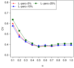
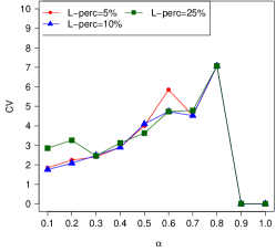
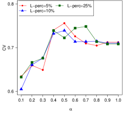
(a) outdegree	(b) betweenness	(c) coreness
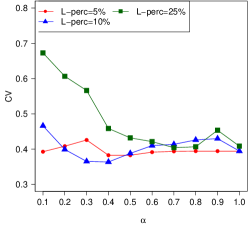
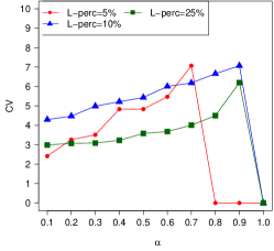
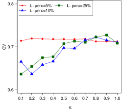
(d) outdegree	(e) betweenness	(f) coreness

Figure 8: Coefficient of variation (CV) of topological properties of identified seed nodes, with $k=50$, by varying $\alpha$ and $L\textit{-perc}$, on GooglePlus: (a)–(c) L-DTIM, (d)–(f) G-DTIM.

Figure 8 shows the coefficient of variation (hereinafter denoted as CV) of selected topological measures over the seed nodes, by varying $\alpha$ and target set size ($L\textit{-perc}$). Looking at results on the outdegree, we observe decreasing trends for CV by increasing $\alpha$ up to 0.5, followed by roughly constant trends set around 0.4, for both DTIM methods. Consistently with the analysis on seed set overlap, L-DTIM seeds tend to have similar outdegree regardless of $L\textit{-perc}$, while in the case of G-DTIM, relatively small variations occur for $L\textit{-perc}=\{5\%,10\%\}$ by varying $\alpha$. As concerns betweenness, CV generally increases with $\alpha$ up to high values (0.7, 0.9), then drastically reduces to zero; this indicates that when diversity is discarded, seeds tend to correspond to source nodes in the graph. Analogously to the outdegree analysis, the trends for varying $L\textit{-perc}$ are quite similar to each other in the L-DTIM case. Considering coreness, CV ranges within a much smaller interval than that corresponding to outdegree and betweenness, i.e., (0.6, 0.76) with L-DTIM, (0.64, 0.73) with G-DTIM. Again, the variability over the seeds computed by L-DTIM is much less affected by the setting of $L\textit{-perc}$ than in the G-DTIM case, with a general increasing trend up to mid-high values of $\alpha$.

As concerns the competing methods, KB-TIM identifies seed nodes having average CV that does not significantly change in terms of $L\textit{-perc}$, specifically: (0.42, 0.40) for outdegree, (3.41, 3.52) for betweenness, and 0.61 for coreness. TIM+ identifies seed nodes that have on average 0.45 CV of outdegree, 0.0 CV of betweenness, and 0.70 CV of coreness.

D.2 Target activation probabilities

In this section we report detailed results concerning the analysis of the target activation probabilities (cf. Section 6.2.2 in the main paper) with the aim of deepening our understanding of how different settings of $\alpha$ impact on the activation probability of nodes targeted by DTIM. We regard the activation probability of a node as the number of times the node has been activated divided by the number of Monte Carlo runs ($I_{MC}$, cf. Algorithm 2).

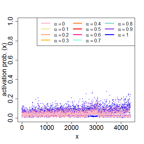
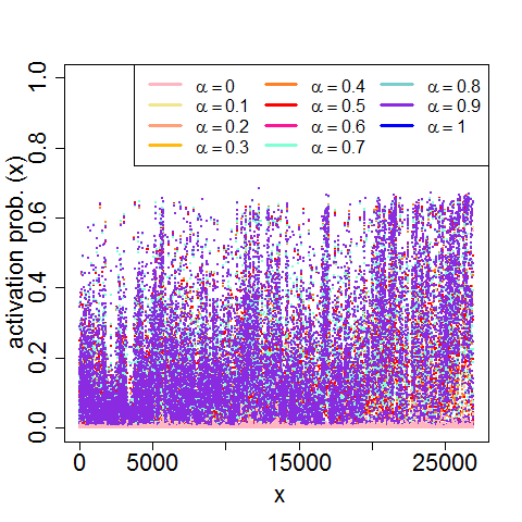
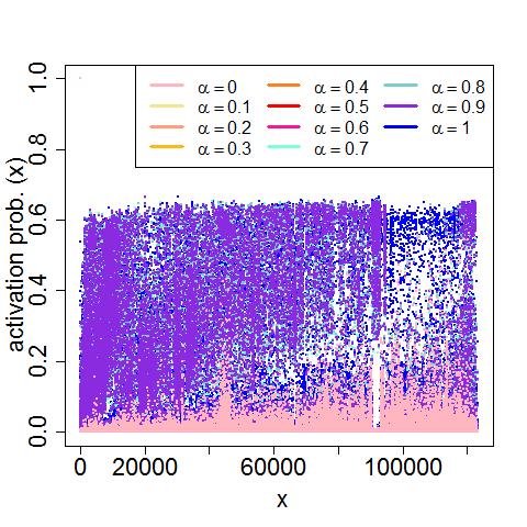
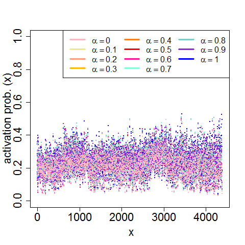
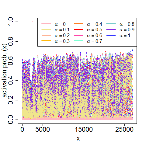
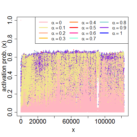
(a)	(b)	(c)

Figure 9: Activation probabilities (y-axis) for each target node (x-axis), obtained by G-DTIM for varying $\alpha$. Results correspond to $L\textit{-perc}=25\%$, $k$ set to $5$ (top) and $50$ (bottom), on (a) Instagram-LCC, (b) GooglePlus, and (c) FriendFeed.

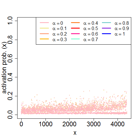
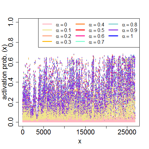
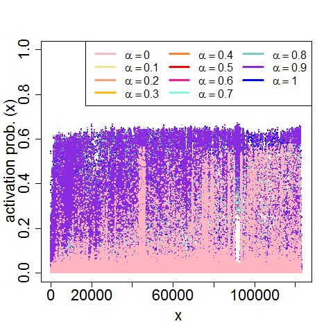
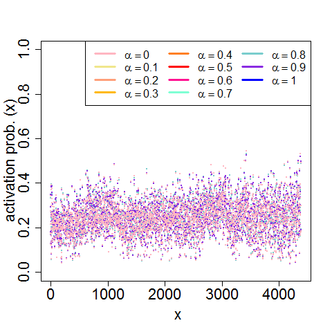
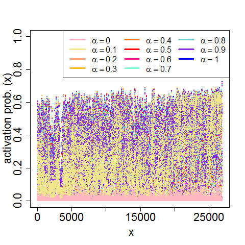
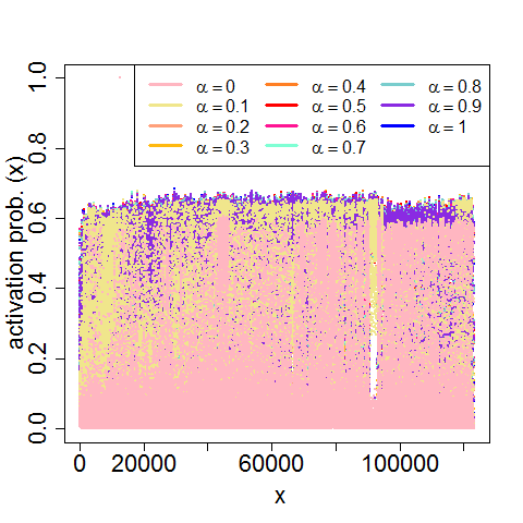
(a)	(b)	(c)

Figure 10: Activation probabilities (y-axis) for each target node (x-axis), obtained by L-DTIM for varying $\alpha$. Results correspond to $L\textit{-perc}=25\%$, $k$ set to $5$ (top) and $50$ (bottom), on (a) Instagram-LCC, (b) GooglePlus, and (c) FriendFeed.

In order to analyze the above property of target nodes, we present first the activation probability values of the nodes in the final active set, shown in Figures 9 and 10. Next we discuss the density distributions $pdf(x)$ with variable $x$ modeling the vector of activation probabilities associated with the nodes in the final active set, reported in Figures 11 and 12.

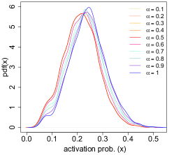
(a)

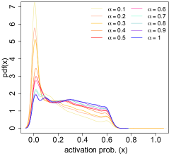
(b)

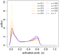
(c)

Figure 11: Density distributions of activation probabilities obtained by G-DTIM, for varying $\alpha$, with $L\textit{-perc}$ set to 25%, $k=50$, on (a) Instagram-LCC, (b) GooglePlus, and (c) FriendFeed.

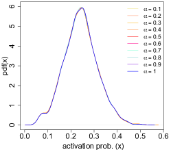
(a)

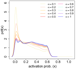
(b)

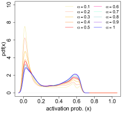
(c)

Figure 12: Density distributions of activation probabilities obtained by L-DTIM, for varying $\alpha$, with $L\textit{-perc}$ set to 25%, $k=50$, on (a) Instagram-LCC, (b) GooglePlus, and (c) FriendFeed.

Plots of activation probability distributions.  Figures 9 and 10 show the activation probabilities versus the target nodes, by varying the values of $\alpha$ and $k$, for G-DTIM and L-DTIM.

Considering first the performance of G-DTIM (Fig. 9), there is an evident gap between the activation probabilities obtained for low $\alpha$ (i.e., $\alpha\leq 0.4$), and higher values of the parameter, with the maximum activation probability values (and maximum coverage of the target set) generally obtained for $\alpha=0.9$ and $\alpha=1.0$. On Instagram-LCC (Fig. 9(a)), given the generally low values of activation probabilities, and the high overlap among the seed sets obtained when varying $\alpha$, the gap between minimum and maximum values is strongly reduced w.r.t. other datasets, with $\alpha=1.0$ showing only small increase on the activation of targets w.r.t. $\alpha=0.0$. Note also that for $k=50$, there is a very small number of nodes showing activation probability within $[0.0,0.1]$: this would hint that, when estimating the activation probabilities, the set of activated nodes remains almost unaffected in all the R Monte Carlo runs (while in other cases there are a bunch of nodes which are reached by the influence diffusion process only for a small number of runs, resulting in near-zero activation probabilities). More interesting behaviors are observed for GooglePlus (Fig. 9(b)). For $k=5$ (upper plot), mid-high activation probabilities are reached for a small set of nodes starting from $\alpha=0.5$, but the majority of target nodes is activated for $\alpha\geq 0.9$, with activation probabilities in the range $[0.0,0.6]$. However, for $k=50$ (lower plot), a significant set of target nodes shows mid-high activation probabilities already for $\alpha=0.1$, indicating that, with a relatively large $k$, low values of $\alpha$ are sufficient to activate target nodes while taking into account diversity. As regards FriendFeed (Fig. 9(c)), activation probabilities obtained for $0.0\leq\alpha\leq 0.6$ are generally higher than the ones obtained for the other two datasets. Nevertheless, for $k=5$ (upper plot), a value of $\alpha=0.7$ is needed to reach significant activation probabilities on a vast portion of the target set. Most target nodes are again reached for $\alpha=0.9$, but it can be noted that there is a large band of target nodes (on the right side of the plot) which reaches mid-high probabilities only for $\alpha=1.0$. This indicates that in large networks, when using low $k$, even small variations on the value of $\alpha$ can significantly impact on the effectiveness of the influence maximization process. Looking at the results obtained for $k=50$ (lower plot), we observe that the set of target nodes obtaining a significant activation probability is relevant already for $\alpha=0.0$, with a coverage on a large portion of the target set starting for $\alpha=0.1$.

Quite similar qualitative remarks can be drawn about the performance of L-DTIM (Fig. 10). As regards Instagram-LCC (Fig. 10(a)), for $k=5$ (upper plot) no visible improvement in the activation probabilities can be observed starting from $\alpha\geq 0.1$, while the results are similar to the ones discussed for G-DTIM for $k=50$ (lower plot). On GooglePlus (Fig. 10(b)), a general improvement of the performance obtained for $\alpha=0.1$ can be noted, while the results obtained for different $\alpha$ values are similar to the ones observed for G-DTIM. The improvement is more evident for $k=5$ (upper plot), but remains significant also for $k=50$ (lower plot). On FriendFeed, an increment in the activation probability values obtained for $0.0\leq\alpha\leq 0.5$ can be noted for $k=5$ (upper plot), w.r.t. the situation described for G-DTIM. With $k=50$ (lower plot), higher probabilities than the ones observed for G-DTIM are observed for $\alpha=0.0$.

Density distributions of activation probability.  Figures 11 and 12 show density distributions of activation probability obtained for G-DTIM and L-DTIM, respectively.

Focusing first on GooglePlus, similar trends can be noted for both G-DTIM (Fig. 11(b)) and L-DTIM (Fig. 12(b)). A density peak corresponding to low activation probability values (close to $0.0$) can be noted for low values of $\alpha$ (i.e., $\alpha\leq 0.6$ for G-DTIM and $\alpha\leq 0.4$ for L-DTIM). This peak slightly decreases for increasing values of $\alpha$, yielding a relatively wide area of nearly constant density (e.g., around $2$) which covers a range of activation probabilities from $0.0$ up to about $0.6$.

A roughly bi-modal distribution can be observed for FriendFeed, for both G-DTIM (Fig. 11(c)) and L-DTIM (Fig. 12(c)). It is easy to recognize a first peak corresponding to near-zero activation probability values, and a second one located around $0.6$; hence, the first peak becomes lower and the second peak higher by increasing $\alpha$.

Analogously to previous evaluation settings, situation on Instagram-LCC is drastically different from the other two datasets, which in this case corresponds to roughly Normal distributions for varying $\alpha$. Using G-DTIM (Fig. 11(a)), the density distribution has a mean activation probability which spans from approximately $0.2$ for low values of $\alpha$ to values close to $0.3$ for higher values of $\alpha$. Using L-DTIM (Fig. 11(b)), due to the high overlap of the seed sets obtained when varying $\alpha$, all distributions are nearly identical, and centered on an average value of activation probability around $0.25$.

It should be noted that the density distributions referring to the setting $\alpha=0.0$ are omitted from Figures 11 and 12. The reason behind this choice is that, as discussed in the previous analysis, in some cases there is a large gap between the activation probabilities obtained with $\alpha=0.0$ and $\alpha=0.1$. Here the entity of such a gap causes the curve of density distribution for $\alpha=0.0$ to have a peak corresponding to very high values of probability density function for near-zero values of activation probability (which, if showed, would force us to use a larger scale, making the other curves difficult to read). This contingency is observed on GooglePlus for both versions of DTIM, and FriendFeed for G-DTIM, while in other cases the density curve for $\alpha=0.0$ can be relatively close (FriendFeed with L-DTIM) or nearly identical (Instagram-LCC for G-DTIM and L-DTIM) to the curve shown for $\alpha=0.1$.

D.3 Correlation analysis between capital and diversity measurements

Tables II and III summarize results of correlation analysis between the sequence of capital values and the sequence of diversity values associated to the nodes at convergence of the diffusion process, for each of the DTIM methods and for selected settings of parameters.

TABLE II: Correlation analysis between capital and diversity measurements: G-DTIM

network	$\alpha$	$L\textit{-perc}$	$k$	correlation
		$(\%)$
GooglePlus	0.1	10	5	-0.001
GooglePlus	0.5	10	5	-0.004
GooglePlus	0.9	10	5	-0.005
GooglePlus	0.1	25	5	0.006
GooglePlus	0.5	25	5	-0.001
GooglePlus	0.9	25	5	-0.006
FriendFeed	0.1	10	5	-4.4e-05
FriendFeed	0.5	10	5	-7.8e-05
FriendFeed	0.9	10	5	-8.1e-05
FriendFeed	0.1	25	5	0.004
FriendFeed	0.5	25	5	0.003
FriendFeed	0.9	25	5	0.001
GooglePlus	0.1	10	50	-0.008
GooglePlus	0.5	10	50	-0.008
GooglePlus	0.9	10	50	-0.007
GooglePlus	0.1	25	50	-0.008
GooglePlus	0.5	25	50	-0.006
GooglePlus	0.9	25	50	-0.011
FriendFeed	0.1	10	50	-1.6e-04
FriendFeed	0.5	10	50	-2.3e-04
FriendFeed	0.9	10	50	-2.7e-04
FriendFeed	0.1	25	50	5.5e-04
FriendFeed	0.5	25	50	3.0e-04
FriendFeed	0.9	25	50	3.3e-04

TABLE III: Correlation analysis between capital and diversity measurements: L-DTIM

network	$\alpha$	$L\textit{-perc}$	$k$	correlation
		$(\%)$
GooglePlus	0.1	10	5	0.169
GooglePlus	0.5	10	5	0.059
GooglePlus	0.9	10	5	0.008
GooglePlus	0.1	25	5	0.148
GooglePlus	0.5	25	5	0.054
GooglePlus	0.9	25	5	0.004
FriendFeed	0.1	10	5	0.085
FriendFeed	0.5	10	5	0.046
FriendFeed	0.9	10	5	0.018
FriendFeed	0.1	25	5	0.076
FriendFeed	0.5	25	5	0.052
FriendFeed	0.9	25	5	0.020
GooglePlus	0.1	10	50	0.225
GooglePlus	0.5	10	50	0.088
GooglePlus	0.9	10	50	0.025
GooglePlus	0.1	25	50	0.229
GooglePlus	0.5	25	50	0.097
GooglePlus	0.9	25	50	0.020
FriendFeed	0.1	10	50	0.164
FriendFeed	0.5	10	50	0.126
FriendFeed	0.9	10	50	0.069
FriendFeed	0.1	25	50	0.180
FriendFeed	0.5	25	50	0.131
FriendFeed	0.9	25	50	0.064

Antonio Caliò is a first-year PhD student in information and communication technologies with the DIMES Department, University of Calabria, Italy. His research interests are focused on information diffusion models, influence propagation, and related computational problems in network and data science.

Roberto Interdonato is a research scientist at Cirad, UMR TETIS, Montpellier, France. He was a postdoctoral researcher with the University of La Rochelle (France), Uppsala University (Sweden), and University of Calabria (Italy), where he received his PhD degree in computer and systems engineering in 2015. His research interests include topics in data mining and machine learning applied to complex networks analysis and to remote sensing analysis.

Chiara Pulice received the PhD degree in computer and systems engineering from the University of Calabria, Italy. She was a visiting scholar at the Department of Computer Science of the University of British Columbia (2013-2014), and a postdoctoral researcher with the University of Maryland’s Institute for Advanced Computer Studies (2016-2017). Currently, she is a postdoctoral researcher with the Dartmouth College Department of Computer Science in Hanover, New Hampshire. Her research interests include data integration, inconsistent databases, data mining, machine learning, and social network analysis.

Andrea Tagarelli is an associate professor of computer engineering at the University of Calabria, Italy. From the same university, he received his PhD degree in computer and systems engineering in 2006. His research interests are in the areas of data mining, machine learning, network analysis, web and semistructured data management, information retrieval. On these topics, he has co-authored about 100 peer-reviewed papers, and edited one book on XML data mining. He co-organized workshops on data mining topics in premier conferences in the field (ACM SIGKDD, SIAM DM, PAKDD, ECML-PKDD, ECIR). He is co-program-chair of the 2018 IEEE/ACM ASONAM Conference.

References

- [1] D. Kempe, J. M. Kleinberg, and E. Tardos, “Maximizing the spread of influence through a social network,” in Proc. ACM KDD, 2003, pp. 137–146.
- [2] A. Goyal, W. Lu, and L. V. S. Lakshmanan, “SIMPATH: An Efficient Algorithm for Influence Maximization under the Linear Threshold Model,” in Proc. IEEE ICDM, 2011, pp. 211–220.
- [3] Y. Tang, X. Xiao, and Y. Shi, “Influence maximization: near-optimal time complexity meets practical efficiency,” in Proc. ACM SIGMOD, 2014, pp. 75–86.
- [4] S. Galhotra, A. Arora, S. Virinchi, and S. Roy, “ASIM: A Scalable Algorithm for Influence Maximization under the Independent Cascade Model,” in Proc. WWW, 2015, pp. 35–36.
- [5] H. Li, S. S. Bhowmick, A. Sun, and J. Cui, “Conformity-aware influence maximization in online social networks,” The VLDB Journal, vol. 24, pp. 117–141, 2015.
- [6] C. Zhou, P. Zhang, W. Zang, and L. Guo, “On the Upper Bounds of Spread for Greedy Algorithms in Social Network Influence Maximization”, IEEE Trans. Knowl. Data Eng., vol. 27, no. 10, pp. 2770–2783, 2015.
- [7] F. C. Santos, M. D. Santos, and J. Pacheco, “Social diversity promotes the emergence of cooperation in public goods games,” Nature, vol. 454, pp. 231–216, 2008.
- [8] Z. Pan, Y. Lu, and S. Gupta, “How heterogeneous community engage newcomers? The effect of community diversity on newcomers’ perception of inclusion,” Computers in Human Behavior, vol. 39, pp. 100–111, 2014.
- [9] L. Robert and D. M. Romero, “Crowd size, diversity and performance,” in Proc. ACM CHI, 2015, pp. 1379–1382.
- [10] K. W. Phillips, “How Diversity Makes Us Smarter,” Scientific American, vol. 311, no. 4, 2014.
- [11] M. Drosou, H.V. Jagadish, E. Pitoura, and J. Stoyanovich, “Diversity in Big Data: A Review,” Big Data Special Issue on Social and Technical Trade-Offs, vol. 5, no. 2, pp. 73–84, 2017.
- [12] F. D. Malliaros and M. Vazirgiannis, “To stay or not to stay: modeling engagement dynamics in social graphs,” in Proc. ACM CIKM, 2013, pp. 469–478.
- [13] A. Anderson, D. Huttenlocher, J. Kleinberg, and J. Leskovec, “Steering user behavior with badges,” in Proc. ACM WWW, 2013, pp. 95–106.
- [14] J. Imlawi and D. G. Gregg, “Engagement in online social networks: The impact of self-disclosure and humor,” Int. J. Hum. Comput. Interaction, vol. 30, no. 2, pp. 106–125, 2014.
- [15] N. Sun, P. P.-L. Rau, and L. Ma, “Understanding lurkers in online communities: a literature review,” Computers in Human Behavior, vol. 38, pp. 110–117, 2014.
- [16] D. A. Harrison and K. J. Klein, “What’s the difference? Diversity constructs as separation, variety, or disparity in organizations,” Academy of Management Review, vol. 32, pp. 1199–1228, 2007.
- [17] “Boundary spanning,” in Encyclopedia of Social Network Analysis and Mining, R. Alhajj and J. Rokne, Eds., 2014, p. 82.
- [18] V. Soroka and S. Rafaeli, “Invisible participants: how cultural capital relates to lurking behavior,” in Proc. ACM WWW, 2006, pp. 163–172.
- [19] R. Interdonato, C. Pulice, and A. Tagarelli., “Community-based delurking in social networks,” in Proc. IEEE/ACM ASONAM, 2016, pp. 263–270.
- [20] ——, ““Got to have faith!”: The DEvOTION algorithm for delurking in social networks,” in Proc. IEEE/ACM ASONAM, 2015, pp. 314–319.
- [21] Y. Li, D. Zhang, and K. Tan, “Real-time targeted influence maximization for online advertisements,” PVLDB, vol. 8, no. 10, pp. 1070–1081, 2015.
- [22] R.-H. Li and J. Xu Yu, “Scalable Diversified Ranking on Large Graphs,” IEEE Trans. Knowl. Data Eng., vol. 25, no. 9, pp. 2133–2146, 2013.
- [23] R. L. T. Santos, C. MacDonald, and I. Ounis, “Search result diversification,” Foundations and Trends in Information Retrieval, vol. 9, no. 1, pp. 1–90, 2015.
- [24] L. Wu, Q. Liu, E. Chen, N. J. Yuan, G. Guo, and X. Xie, “Relevance meets coverage: A unified framework to generate diversified recommendations,” ACM TIST, vol. 7, no. 3, p. 39, 2016.
- [25] J. Kunegis, S. Sizov, F. Schwagereit, and D. Fay, “Diversity dynamics in online networks,” in Proc. ACM HT, 2012, pp. 255–264.
- [26] Q. Bao, W. K. Cheung, and Y. Zhang, “Incorporating structural diversity of neighbors in a diffusion model for social networks,” in Proc. IEEE/WIC/ACM Web Intelligence, 2013, pp. 431–438.
- [27] Y.-H. Fu, C.-Y. Huang, and C.-T. Sun, “Using global diversity and local topology features to identify influential network spreaders,” Physica A, vol. 433, no. C, pp. 344–355, 2015.
- [28] P. Huang, H. Liu, C. Chen, and P. Cheng, “The impact of social diversity and dynamic influence propagation for identifying influencers in social networks,” in Proc. IEEE/WIC/ACM Web Intelligence, 2013, pp. 410–416.
- [29] F. Tang, Q. Liu, H. Zhu, E. Chen, and F. Zhu, “Diversified social influence maximization,” in Proc. IEEE/ACM ASONAM, 2014, pp. 455–459.
- [30] J. Guo, P. Zhang, C. Zhou, Y. Cao, and L. Guo, “Personalized influence maximization on social networks,” in Proc. ACM CIKM, 2013, pp. 199–208.
- [31] B. Guler, B. Varan, K. Tutuncuoglu, M. S. Nafea, A. A. Zewail, A. Yener, and D. Octeau, “Optimal strategies for targeted influence in signed networks,” in Proc. IEEE/ACM ASONAM, 2014, pp. 906–911.
- [32] D. Yang, H. Hung, W. Lee, and W. Chen, “Maximizing acceptance probability for active friending in online social networks,” in Proc. ACM KDD, 2013, pp. 713–721.
- [33] C. Borgs, M. Brautbar, J. T. Chayes, and B. Lucier, “Maximizing Social Influence in Nearly Optimal Time,” in Proc. ACM-SIAM SODA, 2014, pp. 946–957.
- [34] F.-H. Li, C.-T. Li, and M.-K. Shan, “Labeled Influence Maximization in Social Networks for Target Marketing,” in Proc. PASSAT and IEEE SocialCom, 2011, pp. 560–563.
- [35] Q. Liu, Z. Dong, C. Liu, X. Xie, E. Chen, and H. Xiong, “Social marketing meets targeted customers: A typical user selection and coverage perspective,” in Proc. IEEE ICDM, 2014, pp. 350–359.
- [36] J.-R. Lee and C.-W. Chung, “A Query Approach for Influence Maximization on Specific Users in Social Networks,” IEEE Trans. Knowl. Data Eng., vol. 27, no. 2, pp. 340–353, 2015.
- [37] G. Ma, Q. Liu, L. Wu, and E. Chen, “Identifying Hesitant and Interested Customers for Targeted Social Marketing,” in Proc. PAKDD, 2015, pp. 576–590.
- [38] D. J. Watts, “A simple model of global cascades on random networks,” PNAS, vol. 99, pp. 5766–5771, 2002.
- [39] A. Tagarelli and R. Interdonato, “Lurking in social networks: topology-based analysis and ranking methods,” Social Netw. Analys. Mining, vol. 4, no. 230, p. 27, 2014.
- [40] N. Edelmann, “Reviewing the definitions of “lurkers” and some implications for online research,” Cyberpsychology, Behavior, and Social Networking, vol. 16, no. 9, pp. 645–649, 2013.
- [41] A. Tagarelli and R. Interdonato, ““Who’s out there?”: Identifying and Ranking Lurkers in Social Networks,” in Proc. IEEE/ACM ASONAM, 2013, pp. 215–222.
- [42] ——, “Time-aware analysis and ranking of lurkers in social networks,” Social Netw. Analys. Mining, vol. 5, no. 1, p. 23, 2015.
- [43] F. Celli, F. M. L. D. Lascio, M. Magnani, B. Pacelli, and L. Rossi, “Social Network Data and Practices: The Case of Friendfeed,” in Proc. SBP, 2010, pp. 346–353.
- [44] J. J. McAuley and J. Leskovec, “Learning to Discover Social Circles in Ego Networks,” in Proc. NIPS, 2012, pp. 548–556.