Quasielastic charged-current neutrino scattering in the scaling model with relativistic effective mass

Abstract

We use a recent scaling analysis of the quasielastic electron scattering data from ¹²C to predict the quasielastic charge-changing neutrino scattering cross sections within an uncertainty band. We use a scaling function extracted from a selection of the $(e,e^{\prime})$ cross section data, and an effective nucleon mass inspired by the relativistic mean-field model of nuclear matter. The corresponding super-scaling analysis with relativistic effective mass (SuSAM*) describes a large amount of the electron data lying inside a phenomenological quasielastic band. The effective mass incorporates the enhancement of the transverse current produced by the relativistic mean field. The scaling function incorporates nuclear effects beyond the impulse approximation, in particular meson-exchange currents and short range correlations producing tails in the scaling function. Besides its simplicity, this model describes the neutrino data as reasonably well as other more sophisticated nuclear models.

I Introduction

The analysis of modern accelerator-based neutrino oscillation experiments requires a precise knowledge of the intermediate-energy neutrino-nucleus scattering cross section Mos16 ; Kat17 . The inclusive cross section involves contributions from different channels, which can be grouped into quasielastic (QE) one-nucleon emission, multi-nucleon (2p-2h, …) emission, pion production and other inelastic processes. In particular, QE interactions are key processes for these experiments, but the nuclear models for these neutrino and antineutrino cross sections have large uncertainties Pat18 . There are processes which appear as QE-like in the neutrino detectors, produced by final-state interactions, direct multi-nucleon emission, and others which are not under total control from the theoretical point of view, and require relativistic modeling of complex hadronic final states in the continuum. They therefore limit the reach of current and future oscillation experiments such as T2K Abe11 ; Abe18a ; Abe18b , NOvA Ada16 or DUNE Acc15 . Recent attempts to reduce the model uncertainties have been made by measuring the proton multiplicity of the final states in the T2K Abe18b and ArgoNEUT Pal16 ; Acc14 experiments and also the measurement of neutron multiplicity in ANNIE Bac17 is planned.

Within this state of afairs the acquaintance of the inclusive $(e,e^{\prime})$ cross sections of nuclei becomes a valuable starting point; its prior description should be a very convenient requisite for the neutrino-nucleus interaction models. In fact, the isovector component of the electromagnetic nuclear responses can be related to the vector-vector (VV) component of the weak charged-current responses contributing to the neutrino cross sections for the same intermediate energies. The contribution of the axial current might, in principle, be inferred by starting from any available model capable of describing electron scattering. While results from different groups including effects beyond the impulse approximation have allowed to explain the recent neutrino and antineutrino data Mar09 ; Nie11 ; Gal16 ; Meg16 , systematic differences still persist between these theoretical predictions. It is therefore reasonable to suspect that these differences might be attributed to systematic differences in the description of the $(e,e^{\prime})$ data by the same models.

The goal of this paper is to provide predictions for neutrino cross sections with their systematic error inherited directly from the available $(e,e^{\prime})$ data in the superscaling model with relativistic effective mass (SuSAM*) Ama15 ; Ama17 . The scaling approaches Alb88 ; Day90 ; Don99 are an alternative to more sophisticated microscopical models for predicting the neutrino QE cross section. They use a phenomenological scaling functions extracted from the $(e,e^{\prime})$ data, which encode many effects and assume that the same scaling functions can be used to compute the neutrino cross section Ama05a ; Ama05b by just replacing the electromagnetic currents with the vector and axial ones.

The SuSAM* approach used in this paper is an interesting new alternative to the more traditional superscaling analysis approach (SuSA) of refs. Meg16a ; Meg18 , using different assumptions and definitions for the scaling functions and variables.

SuSAM* is based on the relativistic mean field or Walecka model of nuclear matter Ser86 , containing basic theoretical and phenomenological ingredients such as relativity, gauge invariance and dynamical enhancement of lower Dirac components of the nucleon in the medium due to the scalar and vector potentials. These are known to be good enough to describe the electromagnetic nuclear responses in the QE peak Ros80 .

Recently, we have applied SuSAM* to extract a phenomenological scaling function directly from the cross section $(e,e^{\prime})$ data in the QE region within an uncertainty band Ama17b . In Ama17b ; Con18 we have shown that the extracted scaling function $f^{*}(\psi^{*})$ is an universal function valid for all the nuclei, provided that a relativistic effective mass $M^{*}$ and Fermi momentum $k_{F}$ are fitted to the data for each nucleus. These two parameters, $k_{F}$ and $M^{*}$, have been determined in Ama17b from the $(e,e^{\prime})$ database representing a first direct extraction of the Fermi-momentum dependence of relativistic effective mass below saturation from finite nuclei. We find that a subset of a third of the about 20000 existing data approximately scales to an universal superscaling function. The resulting scaling function and its uncertainty band have been parameterized and can thus be easily and directly applied to predict the neutrino QE cross sections within a corresponding uncertainty.

Before proceeding further a qualitying remark regarding interpretation of the present work is in order. From our point of view the SuSAM* band can be understood as the uncertainty in the theoretical description of the QE data due to processes violating the scaling model assumptions. Namely, those interactions which are beyond the impulse approximation and break the factorization of the cross section, but that imply small corrections to the center value and therefore can be regarded as QE-like interactions. The uncertainties obtained in this work for the neutrino cross sections can then be considered most likely as an upper limit to the systematic error expected from nuclear modeling of the QE processes, because all the models aiming to describe the $(e,e^{\prime})$ data should lie inside the phenomenological uncertainty bands for the pertinent kinematics.

The structure of this work is as follows. In Sect. II we describe the theoretical formalism of the SuSAM* model and the parameters of the phenomenological superscaling function $f^{*}(\psi^{*})$. In Sect. III we give our results for the neutrino and antineutrino cross sections and theoretical uncertainties and compare with most of the available data sets. In sect. IV we give our summary and conclusions. In the appendices we show some technical details on the calculation of selected differential cross sections.

II Formalism of quasielastic neutrino scattering

II.1 Cross section and responses

In this paper we are interested in the charged-current quasielastic (CCQE) reactions in nuclei induced by neutrinos. In particular we compute the $(\nu_{\mu},\mu^{-})$ cross section. The total energies of the incident neutrino and detected muon are $\epsilon=E_{\nu}$, $\epsilon^{\prime}=m_{\mu}+T_{\mu}$, and their momenta are ${\bf k},{\bf k}^{\prime}$. The four-momentum transfer is $k^{\mu}-k^{\prime}{}^{\mu}=(\omega,{\bf q})$, with $Q^{2}=q^{2}-\omega^{2}>0$.

If the lepton scattering angle is $\theta_{\mu}$, the double-differential cross section can be written as Ama05a ; Ama05b

$$\frac{d^{2}\sigma}{dT_{\mu}d\cos\theta_{\mu}} = \sigma_{0}\left\{V_{CC}R_{CC}+2{V}_{CL}R_{CL}\right.$$ (1)

$$\left.+{V}_{LL}R_{LL}+{V}_{T}R_{T}\pm 2{V}_{T^{\prime}}R_{T^{\prime}}\right\}\,,$$

where we have defined the cross section

$$\sigma_{0}=\frac{G^{2}\cos^{2}\theta_{c}}{4\pi}\frac{k^{\prime}}{\epsilon}v_{0}.$$ (2)

Here $G=1.166\times 10^{-11}\quad\rm MeV^{-2}\sim 10^{-5}/m_{p}^{2}$ is the Fermi constant, $\theta_{c}$ is the Cabibbo angle, $\cos\theta_{c}=0.975$, and the kinematic factor $v_{0}=(\epsilon+\epsilon^{\prime})^{2}-q^{2}$. The nuclear structure is implicitly written as a linear combination of five nuclear response functions, $R_{K}(q,\omega)$, where the fifth response function $R_{T^{\prime}}$ is added (+) for neutrinos and subtracted ($-$) for antineutrinos). The $V_{K}$ coefficients depend only on the lepton kinematics and are independent on the details of the nuclear target. They are defined by

$${V}_{CC} = 1-\delta^{2}\frac{Q^{2}}{v_{0}}$$ (3)

$${V}_{CL} = \frac{\omega}{q}+\frac{\delta^{2}}{\rho^{\prime}}\frac{Q^{2}}{v_{0}}$$ (4)

$${V}_{LL} = \frac{\omega^{2}}{q^{2}}+\left(1+\frac{2\omega}{q\rho^{\prime}}+\rho\delta^{2}\right)\delta^{2}\frac{Q^{2}}{v_{0}}$$ (5)

$${V}_{T} = \frac{Q^{2}}{v_{0}}+\frac{\rho}{2}-\frac{\delta^{2}}{\rho^{\prime}}\left(\frac{\omega}{q}+\frac{1}{2}\rho\rho^{\prime}\delta^{2}\right)\frac{Q^{2}}{v_{0}}$$ (6)

$${V}_{T^{\prime}} = \frac{1}{\rho^{\prime}}\left(1-\frac{\omega\rho^{\prime}}{q}\delta^{2}\right)\frac{Q^{2}}{v_{0}}.$$ (7)

Here we have defined the dimensionless factors $\delta=m_{\mu}/\sqrt{Q^{2}}$, proportional to the muon mass $m_{\mu}$, $\rho=Q^{2}/q^{2}$, and $\rho^{\prime}=q/(\epsilon+\epsilon^{\prime})$.

We evaluate the five nuclear response functions $R_{K}$, $K=CC,CL,LL,T,T^{\prime}$ ($C$=Coulomb, $L$=longitudinal, $T$=transverse) using a coordinate system with the $z$-axis pointing along ${\bf q}$ and the $x$-axis along the transverse component of the incident neutrino. The nuclear response functions in this frame are given by the following components of the hadronic tensor:

$$R_{CC} = W^{00}$$ (8)

$$R_{CL} = -\frac{1}{2}(W^{03}+W^{30})$$ (9)

$$R_{LL} = W^{33}$$ (10)

$$R_{T} = W^{11}+W^{22}$$ (11)

$$R_{T^{\prime}} = -\frac{i}{2}(W^{12}-W^{21}).$$ (12)

II.2 Nuclear matter responses in the RMF

The starting point in this work is the relativistic mean field (RMF) theory of nuclear matter Ser86 , and its reasonable description of the electromagnetic nuclear response in the quasielastic region Ros80 . This model Ser86 describes the nuclear interaction in terms of vector and scalar potentials whose effect is encoded into a relativistic effective mass $m^{*}_{N}$ of the nucleon in the medium.

In this model the hadronic tensor for one particle-one hole (1p-1h) excitations with momentum ${\bf q}$ and energy $\omega$ can be written as

$$W^{\mu\nu}(q,\omega) = \frac{V}{(2\pi)^{3}}\int d^{3}p\delta(E^{\prime}-E-\omega)\frac{(m_{N}^{*})^{2}}{EE^{\prime}}$$ (13)

$$\times 2w^{\mu\nu}_{s.n.}({\bf p}^{\prime},{\bf p})\theta(k_{F}-p)\theta(p^{\prime}-k_{F})$$

where $E=\sqrt{{\bf p}^{2}+m_{N}^{*}{}^{2}}$ is the initial nucleon energy in the mean field. The final momentum of the nucleon is ${\bf p}^{\prime}={\bf p}+{\bf q}$ and its energy is $E^{\prime}=\sqrt{{\bf p}^{\prime}{}^{2}+m_{N}^{*}{}^{2}}$. Note that the initial and final nucleons have the same effective mass $m_{N}^{*}$. The volume $V=3\pi^{2}{\cal N}/k_{F}^{3}$ of the system is related to the Fermi momentum $k_{F}$ and proportional to the number ${\cal N}=N(Z)$ of neutrons (protons) participating in the process for CC neutrino (antineutrino) scattering. Finally the single-nucleon tensor is written in terms of the CC current

$$w^{\mu\nu}_{s.n.}({\bf p}^{\prime},{\bf p})=\frac{1}{2}\sum_{ss^{\prime}}J^{\mu*}({\bf p}^{\prime},{\bf p})J^{\nu}({\bf p}^{\prime},{\bf p})$$ (14)

where $J^{\mu*}$ is the weak current matrix element between positive energy Dirac spinors with mass $m_{N}^{*}$ and normalized to $\overline{u}u=1$. This single nucleon current is the sum of vector and axial-vector terms $J^{\mu}=V^{\mu}-A^{\mu}$ where the vector current is

$$V^{\mu}_{s^{\prime}s}=\overline{u}_{s^{\prime}}({\bf p}^{\prime})\left[2F_{1}^{V}\gamma^{\mu}+2F_{2}^{V}i\sigma^{\mu\nu}\frac{Q_{\nu}}{2m_{N}}\right]u_{s}({\bf p})$$ (15)

where $F_{i}^{V}=(F_{i}^{P}-F_{i}^{N})/2$ are the isovector form factors of the nucleon. The axial current is

$$A^{\mu}_{s^{\prime}s}=\overline{u}_{s^{\prime}}({\bf p}^{\prime})\left[G_{A}\gamma^{\mu}\gamma_{5}+G_{P}\frac{Q^{\mu}}{2m_{N}}\gamma_{5}\right]u_{s}({\bf p})$$ (16)

Note that the free nucleon mass enters in the current operator, which is not modified in the medium. However the initial and final spinors $u_{s}({\bf p})$, and $u_{s^{\prime}}({\bf p}^{\prime})$, correspond to nucleons with relativistic effective mass $m^{*}_{N}$. This modifies the values of the above matrix elements in the nuclear medium with respect to the free values. Thus the vector current operator used in this work, Eq. (15) corresponds to the CC2 prescription for the off-shell extrapolation of the electromagnetic current operator DeF83 .

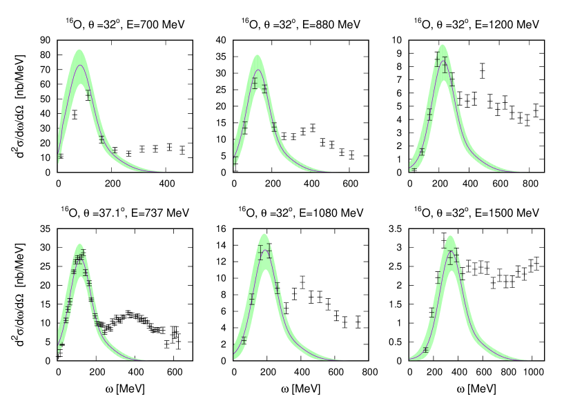
Figure 1: Comparison of inclusive ¹⁶O $(e,e^{\prime})$ cross section and predictions of the SuSAM* model. The solid lines have been obtained with the central parameterization of the scaling function,l while the green band represents the theoretical uncertainty. Data are from Ang96 ; Con87 .

The present RMF theory of nuclear matter treats exactly relativity, gauge invariance and translational invariance. It differs with respect to the well known RFG in that the nucleon mass is replaced by the effective mass both in the spinors and in the energy-momentum relation. As a consequence, equations similar to the RFG responses are obtained by replacing $m_{N}$ by $m_{N}^{*}$ and re-scaling some of the form factors.

The resulting nuclear response function $R_{K}$ is proportional to a single-nucleon response function $U_{K}$ times the scaling function $f^{*}(\psi^{*})$

$$R_{K}=\frac{{\cal N}\xi^{*}_{F}}{m^{*}_{N}\eta_{F}^{*3}\kappa^{*}}U_{K}f^{*}(\psi^{*})$$ (17)

where ${\cal N}$ is the number of neutrons/protons for neutrino/antineutrino scattering, $\eta^{*}_{F}=k_{F}/m^{*}_{N}$, and $\xi^{*}_{F}=\sqrt{1+\eta_{F}^{*2}}-1$. This factorization of the scaling function inspires the scaling models of Alb88 ; Day90 ; Don99 , by using a phenomenological scaling function instead of the well-known scaling function of the Fermi gas

$$f_{\rm RFG}^{*}(\psi^{*})=\frac{3}{4}(1-\psi^{*2})\theta(1-\psi^{*2})\,,$$ (18)

where $\theta$ is the step function and $\psi^{*}$ is the scaling variable. In this work we use a phenomenological scaling function extracted in Ama17 from the $(e,e^{\prime})$ quasielastic data of ¹²C.

In contrast to traditional approaches where the lepton interacts with a free nucleon, here we use a modified scaling variable incorporating the effective mass

$$\psi^{*2}=\frac{1}{\xi^{*}_{F}}{\rm max}\left\{\kappa^{*}\sqrt{1+\frac{1}{\tau^{*}}}-\lambda^{*}-1,\xi^{*}_{F}-2\lambda^{*}\right\}$$ (19)

where $\lambda^{*}=\omega/(2m^{*}_{N})$, $\kappa^{*}=q/(2m^{*}_{N})$, and $\tau^{*}=\kappa^{*2}-\lambda^{*2}$.

The single-nucleon responses $U_{K}$ are obtained analytically by performing the traces in Eq. (14) and the integration in Eq. (13).

The $K=CC$ response is the sum of vector and axial pieces. The vector part implements the conservation of the vector current (CVC), i.e. it vanishes by contracting with $q^{\mu}$. The axial part can be written as the sum of conserved (c.) plus non conserved (n.c.) parts. Then

$$U_{CC} = U_{CC}^{V}+\left(U_{CC}^{A}\right)_{\rm c.}+\left(U_{CC}^{A}\right)_{\rm n.c.}$$ (20)

For the vector CC response we have

$$U_{CC}^{V} = \frac{\kappa^{*2}}{\tau^{*}}\left[(2G_{E}^{*V})^{2}+\frac{(2G_{E}^{*V})^{2}+\tau^{*}(2G_{M}^{*V})^{2}}{1+\tau^{*}}\Delta\right]\ ,$$ (21)

where $G_{E}^{*V}$ and $G_{M}^{*V}$ are the new isovector electric and magnetic nucleon form factors that get modified in the medium through the effective mass:

$$G_{E}^{*V} = F_{1}^{V}-\tau^{*}\frac{m^{*}_{N}}{m_{N}}F_{2}^{V}$$ (22)

$$G_{M}^{*V} = F_{1}^{V}+\frac{m_{N}^{*}}{m_{N}}F_{2}^{V}.$$ (23)

For the free Dirac and Pauli form factors, $F_{1}^{V}$ and $F_{2}^{V}$, we use the Galster parameterization.

The definition of the quantity $\Delta$ in Eq. (21) is

$$\Delta=\frac{\tau^{*}}{\kappa^{*2}}\xi^{*}_{F}(1-\psi^{*2})\left[\kappa^{*}\sqrt{1+\frac{1}{\tau^{*}}}+\frac{\xi^{*}_{F}}{3}(1-\psi^{*2})\right].$$ (24)

The axial-vector CC responses are

$$\left(U_{CC}^{A}\right)_{\rm c.} = \frac{\kappa^{*2}}{\tau^{*}}G_{A}^{2}\Delta$$ (25)

$$\left(U_{CC}^{A}\right)_{\rm n.c.} = \frac{\lambda^{*2}}{\tau^{*}}(G_{A}-\tau^{*}G_{P}^{*})^{2}.$$ (26)

where $G_{A}$ is the nucleon axial-vector form factor and $G_{P}^{*}$ is the new pseudo-scalar axial form factor, also modified in the medium. From partial conservation of the axial current (PCAC), the new and re-scaled pseudo-scalar form factor are now

$$G^{*}_{P}=\frac{4m_{N}m_{N}^{*}}{m_{\pi}^{2}+Q^{2}}G_{A}.$$ (27)

Note that the axial form factor $G_{A}$ is not modified in the medium because in its definition in the axial current, Eq. (16), the nucleon mass does not appear explicitly.

Using current conservation we have for $K=CL,LL$

$$U_{CL} = -\frac{\lambda^{*}}{\kappa^{*}}\left[U_{CC}^{V}+\left(U_{CC}^{A}\right)_{\rm c.}\right]+\left(U_{CL}^{A}\right)_{\rm n.c.}$$ (28)

$$U_{LL} = \frac{\lambda^{*2}}{\kappa^{*2}}\left[U_{CC}^{V}+\left(U_{CC}^{A}\right)_{\rm c.}\right]+\left(U_{LL}^{A}\right)_{\rm n.c.}\ ,$$ (29)

The n.c. parts are

$$\left(U_{CL}^{A}\right)_{\rm n.c.} = -\frac{\lambda^{*}\kappa^{*}}{\tau^{*}}(G_{A}-\tau^{*}G_{P}^{*})^{2}$$ (30)

$$\left(U_{LL}^{A}\right)_{\rm n.c.} = \frac{\kappa^{*2}}{\tau^{*}}(G_{A}-\tau^{*}G^{*}_{P})^{2}\ .$$ (31)

Finally, the transverse responses are given by

$$U_{T} = U_{T}^{V}+U_{T}^{A}$$ (32)

$$U_{T}^{V} = 2\tau^{*}(2G_{M}^{*V})^{2}+\frac{(2G_{E}^{*V})^{2}+\tau^{*}(2G_{M}^{*V})^{2}}{1+\tau^{*}}\Delta$$ (33)

$$U_{T}^{A} = G_{A}^{2}\left[2(1+\tau^{*})+\Delta\right]$$ (34)

$$U_{T^{\prime}} = 2G_{A}(2G_{M}^{*V})\sqrt{\tau^{*}(1+\tau^{*})}[1+\tilde{\Delta}]$$ (35)

with

$$\tilde{\Delta}=\sqrt{\frac{\tau^{*}}{1+\tau^{*}}}\frac{\xi^{*}_{F}(1-\psi^{*2})}{2\kappa^{*}}\ .$$ (36)

II.3 SuSAM* scaling function

One of the inputs of our model is the phenomenological scaling function $f^{*}(\psi^{*})$. This has been determined from a scaling analysis of the quasielastic electron scattering data Ama17 ; Ama15 based on the RMF formulae of the previous section, with an effective mass for the nucleon, in contrast to all previous investigations made with $M^{*}=1$ Day90 ; Don99 ; Ama05a . This analysis allows to select a subset of “quasielastic” data which merge into a thick band that can be separated from the rest of data. This subset turns out to be a large fraction (about a third) of the total 20000 data and approximately scales to an universal superscaling function with uncertainties. The central value of the phenomenological quasielastic band has been parameterized as a sum of two Gaussian functions

$$f^{*}(\psi^{*})=a_{3}e^{-(\psi^{*}-a_{1})^{2}/(2a_{2}^{2})}+b_{3}e^{-(\psi^{*}-b_{1})^{2}/(2b_{2}^{2})}.$$ (37)

The coefficients encoding the band and their ranges are provided in table 1. The lower and upper limits of the phenomenological band have been parameterized as sum of two Gaussians as well, with coefficients $a_{i}^{min/max}$, $b_{i}^{min/max}$, given in table 1 too. Note that the new scaling function $f^{*}(\psi^{*})$ is different to the phenomenological scaling function used in the SuSA formalism Mai02 .

	$a_{1}$	$a_{2}$	$a_{3}$	$b_{1}$	$b_{2}$	$b_{3}$
central	-0.0465	0.469	0.633	0.707	1.073	0.202
min	-0.0270	0.442	0.598	0.967	0.705	0.149
max	-0.0779	0.561	0.760	0.965	1.279	0.200

Table 1: Parameters of our fit of the phenomenological scaling function central value, $f^{*}(\psi^{*})$, and of the lower and upper boundaries (min and max, respectively).

The present SuSAM* model provides a landmark representation of the intermediate energy quasielastic data, in the sense that any model aiming to describe these quasielastic data should lie inside the uncertainty band. It gives a fair and simple description of the selected data band. Besides the scaling function $f^{*}(\psi^{*})$, it only includes two parameters: the effective mass and the Fermi momentum.

In the present work we will apply this model to neutrino and antineutrino quasielastic scattering from ¹²C and ¹⁶O, assuming the same uncertainty band in the scaling function as determined in $(e,e^{\prime})$. In ref. Ama17 we showed the results of our model for the doubly differential ¹²C$(e,e^{\prime})$ cross section, with a fair global description of data. In Fig. 1 we compare our model with the ¹⁶O data. We remark that only six kinematics are available for this nucleus. We use the values $M^{*}=0.8$ and $k_{F}=230$ MeV/c, taken from the recent $A$-dependent super-scaling analysis of Ama17b , while the scaling function band is the same as that of ¹²C determined in Ama17 and given in Table 1.

As it can be observed most of the data around the quasielastic region are well described. Note that our model does not include the pion emission or inelastic channels and therefore the higher energy data lie, as expected, outside our uncertainty band. The quality of our description is similar to the one of the SuSAv2 model Meg16a ; Meg18 . In addition, we provide an estimation of the theoretical error in the cross section, that will be translated to neutrino cross section error bands in the results of the next section.

III NUMERICAL PREDICTIONS

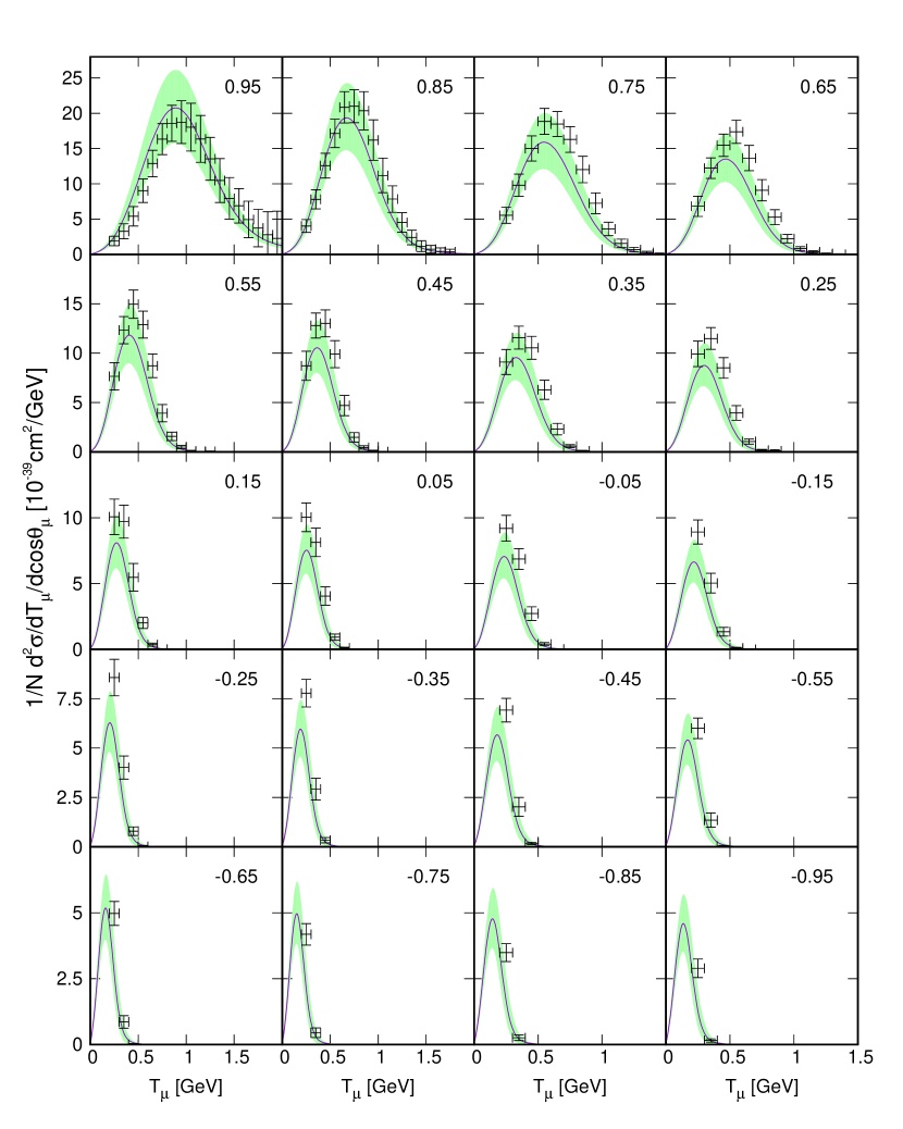
Figure 2: (Color online) Flux-integrated double-differential cross section per target neutron for the CCQE $(\nu_{\mu},\mu^{-})$ reaction on ¹²C in the SuSAM* model. Each panel is labeled by the mean value of $\cos\theta_{\mu}$ in each experimental bin. The experimental data are from Agu10

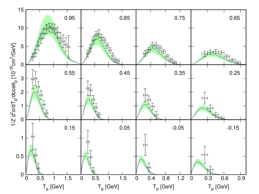
Figure 3: (Color online) Flux-integrated double-differential cross section per target proton for the CCQE $(\bar{\nu}_{\mu},\mu^{+})$ reaction on ¹²C in the SuSAM* model. Each panel is labeled by the mean value of $\cos\theta_{\mu}$ in each experimental bin. The experimental data are from Agu13 .

In this section we present our results for the quasielastic neutrino and antineutrino cross sections on ¹²C and ¹⁶O within the SuSAM* model. The parameters of the model are the effective mass $M^{*}=0.8$ and the Fermi momentum $k_{F}=225$, 230 MeV/c, for carbon and oxygen, respectively. The other input of the model is the phenomenological scaling function $f^{*}(\psi^{*})$, extracted from $(e,e^{\prime})$ data as described in the previous section.

III.1 MiniBooNE

We start with the discussion of the MiniBooNE results Agu10 ; Agu13 . In Fig. 2 we show our results for the flux-averaged double differential cross section

$$\frac{d^{2}\sigma}{dT_{\mu}d\cos\theta_{\mu}}=\frac{1}{\Phi_{tot}}\int dE_{\nu}\Phi(E_{\nu})\frac{d^{2}\sigma}{dT_{\mu}d\cos\theta_{\mu}}(E_{\nu})\,,$$ (38)

where $\frac{d^{2}\sigma}{dT_{\mu}d\cos\theta_{\mu}}(E_{\nu})$ is the computed cross section for fixed neutrino energy $E_{\nu}$. The neutrino flux $\Phi(E_{\nu})$ corresponds to the MiniBooNE experiment on ¹²C nucleus Agu10 .

In the figure the band predictions and the central cross section values are compared to the experimental data of Ref Agu10 , which are given in bins of $\cos\theta_{\mu}$ and $T_{\mu}$. In each panel of Fig. 2 we fix the $\cos\theta_{\mu}$ to the corresponding experimental bin and the cross section is plotted as a function of $T_{\mu}$. In each panel we perform an integration over the corresponding angular window in $\cos\theta_{\mu}$ and divide by the bin width $\Delta\cos\theta_{\mu}=0.1$.

We observe that the strength and peak position are reasonably well described by our model, and that the band thickness is similar to the experimental errors. The data are slightly above our central curves, except for very forward angles ($\cos\theta_{\mu}\sim 0.95$ panel). Thus, we find that, in general, the data are consistent with the band within the experimental errors. Note that, by construction, the band contains by definition the purely QE nuclear effects coming from the $(e,e^{\prime})$ data. This is a very rewarding result which essentially confirms in a quantitative way the underlying hypothesis of the scaling analysis, namely, the fact that around the QE the main difererence between electron and neutrino scattering is mainly due to the different currents and not so much on the intricacies of nuclear effects. Of course, such a description has limitations and is subjected to improvements. Actually, the experimental neutrino data above the QE band indicate the existence of QE-like effects without pions, as 2p-2h meson-exchange currents (MEC) and short-range correlations or $\pi$-emission and reabsorption. Besides, the neutrino data falling slightly below the band for low muon energy in the top left panel point to low-$q$ mechanisms which are, in general, overestimated by the scaling model. All these effects are known to violate scaling and are expected to produce additional contributions to the band results. Our goal here is limited to study the implications of the $(e,e^{\prime})$ band when directly translated to neutrino scattering. The inclusion of these effects, while extremely interesting, is beyond the scope of this work and is left for future research.

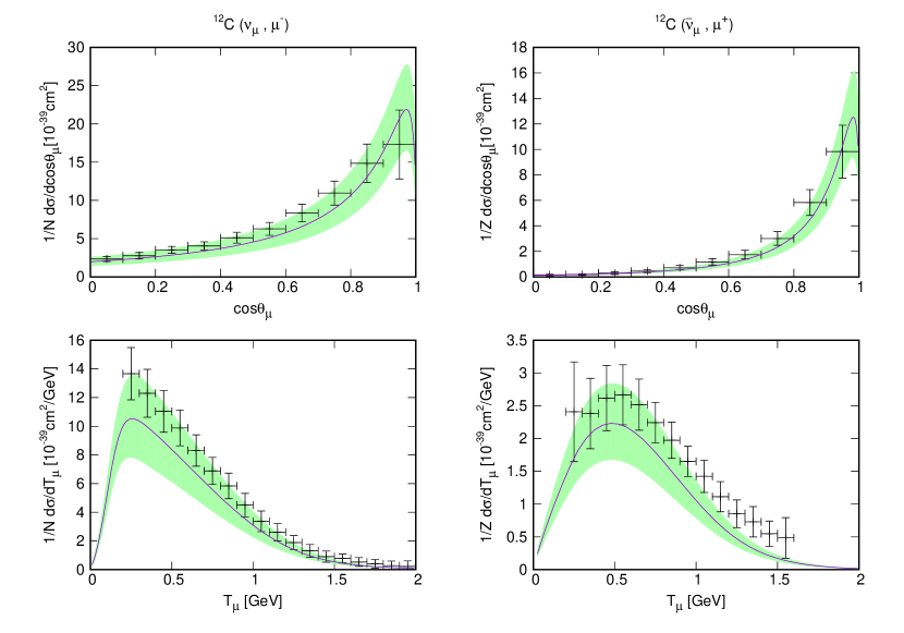
Figure 4: (Color online) Flux-integrated single-differential cross sections per target neutron (proton) for the CCQE neutrino (antineutrino) reactions on ¹²C in the SuSAM* model. Left panels are for neutrinos and right ones for antineutrinos. The experimental data are from Agu10 ; Agu13

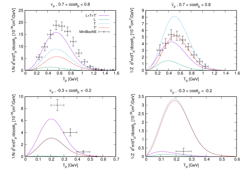
Figure 5: (Color online) Flux-integrated double-differential cross section per target neutron (proton) for the CCQE neutrino (antineutrino) reaction on ¹²C in the SuSAM* model (neutrino left and antineutrino right). The separate contributions of the L, T and T’ responses are highlighted for two selected kinematics. The experimental data are from Agu10 ; Agu13

The antineutrino double differential cross sections for the kinematics of the MiniBooNE experiment Agu13 are shown in Fig. 3. Again a good description of data is observed. In general the data are above our central curves, leaving room for additional nuclear effects not included in the SuSAM* model.

Our results on Figs. 2 and 3 are quantitatively slightly larger than those of the RMF model of Udias et al. Ama11 ; Iva13 , but it is apparent that the RMF is closely inside our uncertainty band. This was to be expected because both models are based on the same theoretical Walecka model Ser86 . The main difference between both approaches is that the model of Udias et al. describes finite nuclei with local vector and scalar potentials, while here our potentials are constant and generate a fixed effective mass inside the volume containing the RFG. In our case the scaling function takes into account the finite size of the nucleus and, besides, it is phenomenological, what accounts for the differences between both models.

Despite the fact that our model is not including 2p-2h explicitly, it is remarkable that the agreement of our central curve with the MiniBooNE data is similar to that obtained with more sophisticated models as those by authors Nieves et al. Nie12 ; Nie13 , Martini et al. Mar11 ; Mar13 , and Mosel et al. Gal16 . This is so because the RMF includes some dynamical relativistic effects like enhancement of transverse response due to lower components of nucleon spinors and other nuclear effects hidden into the phenomenological scaling function $f^{*}(\psi^{*})$.

The uncertainty imposed by the QE $(e,e^{\prime})$ data over neutrino scattering can be globally appreciated in the single differential cross sections of Fig. 4, obtained by integration of the double differential ones. In general the data are within the SuSAM* band. Our central curves are systematically slightly below the data, in agreement with the results of the previous Figs. 2 and 3. The thickness of the band seems larger than in the $(e,e^{\prime})$ cross sections. This appears to be due to the integration over the neutrino flux, which mixes the bands for different kinematics.

A closer insight into our results is considered in Fig. 5. Here we show the separate contributions of the $L$, $T$ and $T^{\prime}$ responses to the cross section for several kinematics. The contribution of $L$ response is considerably smaller than the transverse channels. The $T$ response gives the largest contribution. This indicates that the axial contribution to the transverse cross section is larger than the $VV$ one. For large scattering angle the $T$ and $T^{\prime}$ responses tend to be almost equal. This produces a large cancellation in the antineutrino cross section, which is therefore very small for large angles. Due to this cancellation one would expect the antineutrino cross section to be more sensitive to the details of the longitudinal responses. The results of Fig. 5 are useful to further be compared with those of the RMF model of Udias et al. (see Figs. 2 and 3 of ref. Iva13 ), being in fair agreement with our findings. This comparison again ensures the similitudes between the SuSAM* and the RMF in finite nuclei for intermediate energies.

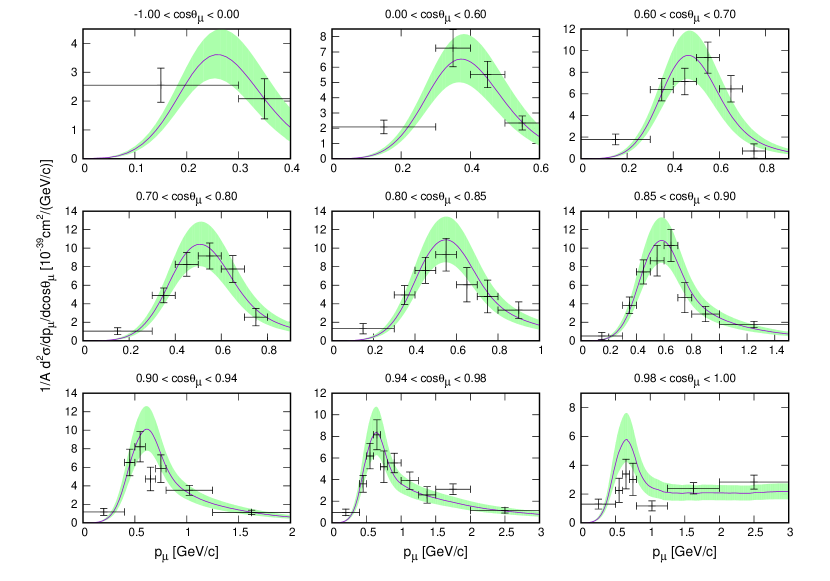
Figure 6: T2K flux-folded double differential CCQE cross section per nucleon for $\nu_{\mu}$ scattering on ¹²C in the SuSAM* model. Experimental data are from Abe16 .

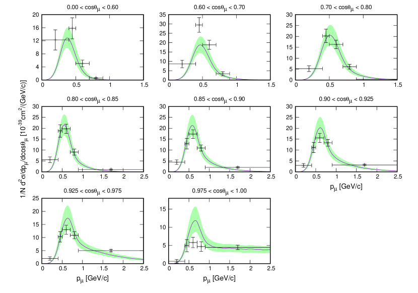
Figure 7: T2K flux-folded double differential CCQE cross section per neutron for $\nu_{\mu}$ scattering on ¹⁶O in the SuSAM* model. Experimental data are from Abe17 .

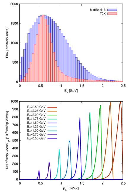
Figure 8: (color online) Top panel: Comparison of MiniBooNE and T2K neutrino fluxes. Bottom panel: Double-differential CCQE ¹⁶O $(\nu_{\mu},\mu^{-})$ cross section for fixed neutrino energies computed for the angular bin $0.975<\cos\theta_{\mu}<1$.

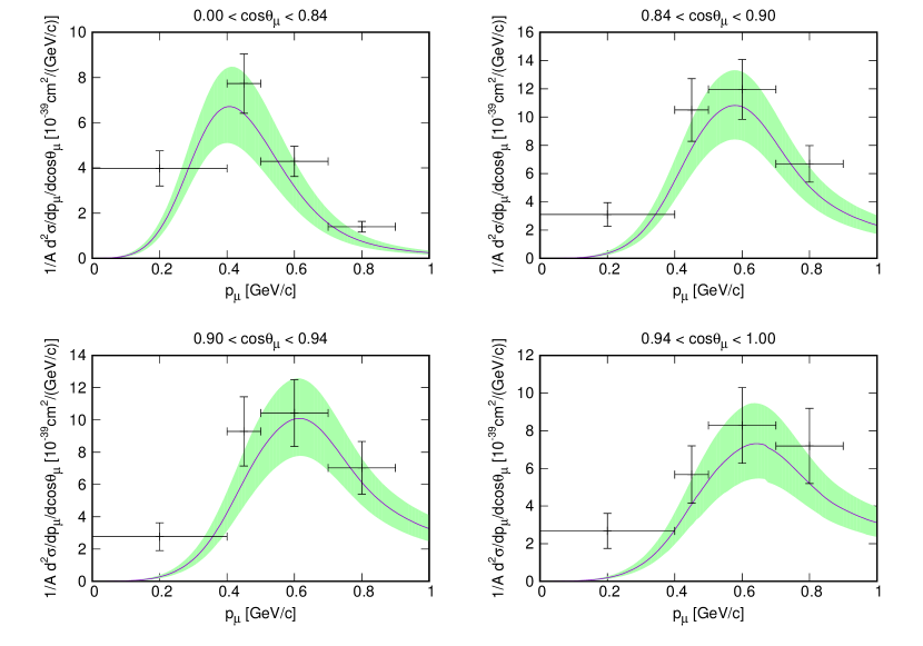
Figure 9: T2K flux-folded double differential CC inclusive cross section per nucleon for $\nu_{\mu}$ scattering on ¹²C in the SuSAM* model. Experimental data are from Abe13 .

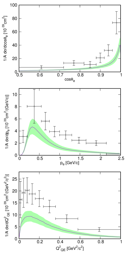
Figure 10: T2K flux-folded single differential CC inclusive cross section per nucleon for $\nu_{e}$ scattering on ¹²C in the SuSAM* model. Experimental data are from Abe14 . The neutron binding energy for this case is $E_{B}=25$ MeV.

III.2 T2K

In Figs. 6 and 7 we compare the SuSAM* predictions with the measurement of double-differential muon neutrino CC cross section without pions (CCQE-like) of the T2K experiment from ¹²C Abe16 and ¹⁶O Abe17 . The experimental data nicely fall inside the QE uncertainty band except for very forward angles, where the data are overestimated around the maximum of the cross section. This is related to the limitations of the SuSAM* model to describe the low momentum transfer region.

In contrast to the MiniBooNE experiment, the T2K data bins are not equally-spaced in $\cos\theta_{\mu}$, and the forward angle dependence is probed in some more detail than in the MiniBooNE analysis. Note that in all the calculations we average the cross section over the corresponding angular bin. The neutrino energy distribution of the T2K experiment is also different from that of the MiniBooNE experiment, the former being narrower around the maximum value $\sim 0.5$ GeV. Both neutrino fluxes are compared in Fig. 8.

The flux folding of the cross section, Eq. (38), implies an integration over the incident neutrino energy, which produces a smearing of the cross section for different energies. This results in a mild model dependence of the QE neutrino cross sections. Being the flux narrower than the MiniBooNE one, one would expect the T2K experiment to be more suited for discriminating over different theoretical models of the reaction. Note also that the T2K angular bins are smaller for small angles ($\cos\theta_{\mu}>0.8$), but for large angles ($\cos\theta_{\mu}<0.6$) the bins are embracing a large angular sector, thus acquiring a larger additional smearing of angular cross sections. For all these reasons, the T2K and MiniBooNE cross sections are not directly comparable because they explore different energy and angular regions of the QE peak by selected integrations.

In Fig. 8 we analyze in more detail the smearing effect produced by the folding with the neutrino flux. We show the QE cross section for fixed neutrino energies $E_{\nu}=0.5,\ldots,2.5$ GeV, as a function of the muon momentum for the kinematics $0.98<\cos\theta_{\mu}<1$ (corresponding to the last panels in Figs. 6 and 7). For fixed neutrino energy, the cross section is a narrow peak contributing to the flux-folded cross section only in a narrow region in $p_{\mu}$. As $E_{\nu}$ increases the allowed muon energy increases and the peak position moves to the right, and its width increases, as a function of $p_{\mu}$. From this figure we can infer that the error of the reconstruction of the neutrino energy from the flux-folded cross section is related to the width of these peaks for fixed neutrino energy —or more precisely for fixed $T_{\mu}$, which is of the same order.

It is interesting to see that the strength of the cross section increases with $E_{\nu}$. This is in contrast to the electron scattering QE cross section, which decreases with the incident electron energy. The reason is because in the electromagnetic interaction there is a photon propagator squared $1/Q^{4}$, which decreases with $Q^{2}$, while in the weak CC case there is a $W^{\pm}$ propagator squared $\simeq 1/M_{W}^{4}$ which is almost constant for the low $Q^{2}$-values considered here. Therefore the neutrino cross section increases with $E_{\mu}$. This increase is partially balanced with a decrease of the neutrino flux inside the folding. Accidentally, this balance turns out to be almost perfect in the case of the T2K experiment for the kinematics of Fig. 8 and that is the reason why for large $p_{\mu}$ the flux-folded cross section does not fall to zero and is almost constant in the last panels of Figs. 6 and 7.

To complete the comparison with T2K data, in Figs. 9 and 10 we compare our model with the data of total inclusive cross sections for $\nu_{\mu}$ Abe13 and $\nu_{e}$ CC scattering from ¹²C Abe14 . Up to now we have compared with inclusive data without pions in the final state (CCQE-0$\pi$), corresponding to QE-like events, but they are not restricted to one-nucleon emission because these semi-inclusive cross sections contain multi-nucleon emission, mainly from 2p-2h final states. Our model accounts for this multi-nucleon emission, at least partially, because the effective mass and scaling function is extracted directly from cross section data. The width of the band should account for those processes that violate scaling, but remain close to the QE peak. In particular, the tail in the scaling function is produced by nucleons with large momentum (compared to $k_{F}$) inside the ground state, which are mainly produce by short-range correlations. Other mechanisms such as meson-exchange currents also should contribute partially to the uncertainty band.

In addition to this, the inclusive neutrino data in Figs. 9 and 10 contain also explicit pion emission and other inelasticities, which do not scale and have been disregarded in our selection of QE $(e,e^{\prime})$ data. That is why our results underestimate the inclusive cross sections, as it is more apparent in the case of $\nu_{e}$, shown in Fig. 10.

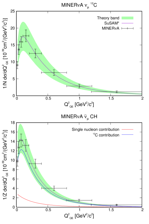
Figure 11: (color online) Flux-folded CCQE $(\nu_{\mu},\mu^{-})$ and $(\bar{\nu}_{\mu},\mu^{+})$ scattering from ¹²C and CH scattering compared to the MINERvA experiment. The H contribution is obtained from the elastic antineutrino-proton cross section divided by $Z=7$. The data are from Bet16 .

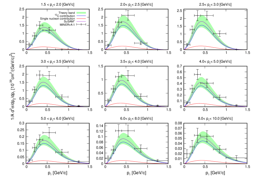
Figure 12: (color online) Flux-folded double-differential cross section $\frac{d^{2}\sigma}{dp_{\parallel}dp_{\perp}}$ for antineutrino CCQE scattering from CH (hydrocarbon) compared to the MINERvA experiment. The H contribution is obtained from the elastic antineutrino-proton cross section divided by $A=13$. The data are from Pat18 .

III.3 MINERvA

In Fig. 11 we show the flux-folded CCQE single-differential cross section $d\sigma/dQ^{2}_{QE}$ for $(\nu_{\mu},\mu^{-})$ and $(\bar{\nu}_{\mu},\mu^{+})$ scattering from ¹²C and CH respectively, compared to the MINERvA experiment Bet16 . This cross section is presented as a function of the reconstructed variable $Q^{2}_{QE}$, which is not the true $Q^{2}$, but it is computed from the reconstructed neutrino energy assuming quasielastic scattering from a nucleon at rest. In Appendix A we show details on how this cross section is computed. The cross section data for antineutrino scattering contain the H contribution from the target. In Appendix B we show how we evaluate this cross section within our formalism. As we can see in Fig. 11, all the MINERvA data fall with our uncertainty band and, moreover, they are very close to the central value of the SuSAM* model predictions.

To finish our discussion, in Fig. 12 we show the double differential antineutrino cross section for QE scattering on CH (hydrocarbon) corresponding to the recent measurements in the MINERvA detector Pat18 .

The double-differential measurements of antineutrino QE scattering in the MINERvA detector provide a complete description of observed muon kinematics with respect to the muon longitudinal and transverse momentum with respect to the incident neutrino. These are related to the variables $p_{\mu},\cos\theta_{\mu}$ by

$$p_{\parallel} = p_{\mu}\cos\theta_{\mu}$$ (39)

$$p_{\perp} = p_{\mu}\sin\theta_{\mu}$$ (40)

It is then straightforward to compute the Jacobian of the transformation to the usual cross section variables $E_{\mu},\cos\theta_{\mu}$

$$dp_{\parallel}dp_{\perp}=\frac{E_{\mu}}{\sin\theta_{\mu}}dE_{\mu}d\cos\theta_{\mu}$$ (41)

Therefore we compute the MINERvA double-differential cross section as

$$\frac{d^{2}\sigma}{dp_{\parallel}dp_{\perp}}=\frac{\sin\theta_{\mu}}{E_{\mu}}\frac{d^{2}\sigma}{dE_{\mu}d\cos\theta_{\mu}}$$ (42)

Our calculation in Fig. 12 is compared with the ’true’ CCQE data from tables XXII, XXIII and XXIV of ref. Pat18 . Most of the data are within the uncertainty band and slightly above the central SuSAM* results. This may indicate the presence of some non-QE events in the data. The hydrogen contribution is also included in the calculation from hydrocarbon. It is found to provide a small correction which slightly increases the cross section, but it could be safely ignored without sensibly modifying the uncertainty band of Fig. 12. Note that in each panel of the figure the parallel component of the muon momentum is averaged over the corresponding experimental bin as indicated. By plotting the cross section as a function of the perpendicular muon momentum not only the total muon momentum increases, but also the angle, opposite to the usual $E_{\mu}$-plots where the $\cos\theta_{\mu}$ bins are kept constant.

IV Conclusions

Summarizing, in this work we have provided predictions for the CCQE neutrino and antineutrino cross sections and their theoretical uncertainties. These uncertainties are extracted directly from the $(e,e^{\prime})$ data and can be considered upper limits to the expected systematic errors coming from the nuclear modeling of the reaction. We have compared our model with the available QE neutrino and antineutrino double-differential and differential cross section data from MiniBooNE, T2K and MINERvA experiments, with a reasonable agreement. The theoretical uncertainty bands are around $20\%-30\%$ and, in general, of the same order as the experimental errors.

The agreement of our central results with data is similar to that obtained with much more sophisticated theoretical models. We emphasize that the results were obtained without any tuning of model parameters except the relativistic effective mass and the Fermi momentum, extracted from a large body of $(e,e^{\prime})$ data around the QE. The accord with data over different experiments, different nuclei, and spanning a wide range of neutrino and antineutrino energies, shows that the SuSAM* uncertainty bands faithfully encode intricate nuclear effects and qualify as a suitable tool for the validation of models of QE-like interactions. We plan to explore ways to reduce the systematic errors, for instance by combining the SuSAM* model with explicit additional contributions from meson-exchange currents, which only are partially included in the phenomenological scaling function, or by extending the model to account for the inelastic channels.

V Acknowledgements

This work has been partially supported by the Spanish Ministerio de Economia y Competitividad (grants Nos. FIS2014-59386-P and FIS2017-85053-C2-1-P) and by the Junta de Andalucia (grant No. FQM-225). V.L.M.C. acknowledges a contract with Universidad de Granada funded by Junta de Andalucia and Fondo Social Europeo.

Appendix A Reconstructed $Q^{2}_{QE}$ differential cross section

A quantity of interest in the experiments is the reconstructed neutrino energy assuming quasielastic scattering on a nucleon at rest. By energy-momentum conservation, it is given by Agu10 ; Pat18 ; Pat18_thesis

$$E_{\nu}^{QE}=\frac{m_{p}^{2}-m^{\prime}_{n}{}^{2}-m_{\mu}^{2}+2m^{\prime}_{n}E_{\mu}}{2(m^{\prime}_{n}-E_{\mu}+p_{\mu}\cos\theta_{\mu})}$$ (43)

where $m_{n}^{\prime}=m_{n}-E_{b}$, and $E_{b}=34$ MeV is an effective binding energy for an initial neutron at rest in ¹²C. For the inverse reaction case of antineutrinos one should exchange the neutron and proton masses in the formula and a change in $E_{b}=30$ MeV. With this, the reconstructed $Q^{2}_{QE}$ is given by

$$Q^{2}_{QE}=2E_{\nu}^{QE}(E_{\mu}-p_{\mu}\cos\theta_{\mu})-m_{\mu}^{2}$$ (44)

Note that the reconstructed variable $Q^{2}_{QE}$ is not the true $Q^{2}$ because the true neutrino energy is unknown. It is a function of $(\cos\theta_{\mu},E_{\mu})$. It is a convenient variable to present results in a representation similar to the neutrino-nucleon cross section. The definition of the cross section $d\sigma/dQ^{2}_{QE}$ is the following

$$\frac{d\sigma}{dQ^{2}_{QE}}=\int dE_{\mu}\frac{\displaystyle\frac{d\sigma}{d\cos\theta_{\mu}dE_{\mu}}}{\left|\displaystyle\frac{\partial Q^{2}_{QE}}{\partial\cos\theta_{\mu}}\right|}$$ (45)

were the cross section in the numerator, is the flux-folded double-differential cross section. The denominator is the Jacobian in the change of variables $(\cos\theta_{\mu},E_{\mu})\rightarrow(Q^{2}_{QE},E_{\mu})$. Therefore inside the integral the $\cos\theta_{\mu}$ variable is computed from Eqs. (43–44) by solving for $\cos\theta_{\mu}$ in terms of the independent variables $(Q^{2}_{QE},E_{\mu})$:

$$\cos\theta_{\mu} = \left[E_{\mu}(m_{p}^{2}-m^{\prime}_{n}\mbox{}^{2}-m_{\mu}^{2}+2m^{\prime}_{n}E_{\mu})\right.$$ (46)

$$-\left.(m_{n}^{\prime}-E_{\mu})(Q^{2}_{QE}+m_{\mu}^{2})\right]$$

$$\times\left[p_{\mu}(Q^{2}_{QE}+m_{p}^{2}-m^{\prime}_{n}\mbox{}^{2}+2m^{\prime}_{n}E_{\mu})\right]^{-1}$$

The Jacobian in the denominator is then given by

$$\kern-8.53581pt\frac{\partial Q^{2}_{QE}}{\partial\cos\theta_{\mu}} = 2\frac{\partial E_{\nu}^{QE}}{\partial\cos\theta_{\mu}}(E_{\mu}-p_{\mu}\cos\theta_{\mu})-2p_{\mu}E_{\nu}^{QE}$$ (47)

$$\kern-8.53581pt\frac{\partial E_{\nu}^{QE}}{\partial\cos\theta_{\mu}} = -\frac{m_{p}^{2}-m^{\prime}_{n}\mbox{}^{2}-m_{\mu}^{2}+2m^{\prime}_{n}E_{\mu}}{2(m^{\prime}_{n}-E_{\mu}+p_{\mu}\cos\theta_{\mu})^{2}}p_{\mu}.$$ (48)

The resulting differential cross section has been computed using (A3) when we compare with the MINERvA data.

Appendix B The elastic $p(\bar{\nu}_{\mu},\mu^{+})n$ cross section

Some experiments provide cross sections including the contributions from the Hydrogen target atoms. Therefore, when comparing with such experiments, such as the MINERvA data, the individual proton cross sections have to be added incoherently to the ¹²C one in proportion to the relative number of protons in each species of the target.

Here we compute this contribution as a particular case of the RFG formalism for $k_{F}=0$, $Z=1$ and $M^{*}=1$. For the flux averaged antineutrino cross section we have

$$\frac{d^{2}\sigma}{dT_{\mu}d\cos\theta_{\mu}} = \int dE_{\nu}\phi(E_{\nu})\frac{m_{n}}{E^{\prime}}\delta(E^{\prime}+E_{\mu}-m_{p}-E_{\nu})$$ (49)

$$\times\sigma_{0}(E_{\nu})\sum_{K}V_{K}U^{K}(E^{\prime},0),$$

where the elastic single nucleon responses $U^{K}(E^{\prime},0)$ are evaluated for a nucleon at rest using Eqs. (20, 28, 29, 32, 35), for $k_{F}=0$, or equivalently, by simply setting $\Delta=\tilde{\Delta}=0$ in those equations. Being a nucleon at rest, the values of $q$ and $\omega$ are calculated from the kinematics inside the integral. To integrate over the neutrino energy using the Dirac delta, we take into account that the final nucleon energy, $E^{\prime}$, depends on the antineutrino energy through

$$E^{\prime}{}^{2}=m_{n}^{2}+E_{\nu}^{2}+p_{\mu}^{2}-2E_{\nu}p_{\mu}\cos\theta_{\mu}$$ (50)

Differentiating we can write

$$\frac{dE_{\nu}}{E^{\prime}}=\frac{d(E^{\prime}-E_{\nu})}{E_{\nu}-p_{\mu}\cos\theta_{\mu}-E^{\prime}}.$$ (51)

Now it is straightforward to integrate the Dirac delta, obtaining

$$\frac{d^{2}\sigma}{dT_{\mu}d\cos\theta_{\mu}} = \phi(E_{\nu})\frac{m_{n}}{|E_{\mu}-m_{p}-p_{\mu}\cos\theta_{\mu}|}$$ (52)

$$\times\sigma_{0}(E_{\nu})\sum_{K}V_{K}U^{K}(E^{\prime},0),$$

where we have taken the absolute value of the Jacobian and replaced in the denominator $E_{\nu}-E^{\prime}=E_{\mu}-m_{p}$. The value of the antineutrino energy is

$$E_{\nu}=\frac{m_{n}^{2}-m_{p}^{2}-m_{\mu}^{2}+2m_{p}E_{\mu}}{2(m_{p}-E_{\mu}+p_{\mu}\cos\theta_{\mu})}$$ (53)

and $E^{\prime}=E_{\nu}-E_{\mu}+m_{p}$. This solves the double-differential cross section problem. Finally, to compute the single differential cross section $d\sigma/dQ^{2}_{QE}$ for the proton we apply again the method explained in Appendix A, for $E_{b}=0$.

References

- (1) U. Mosel, Ann. Rev. Nuc. Part. Sci. 66 (2016), 171.
- (2) T. Katori and M. Martini, J. Phys. G 45 (2018) no.1, 013001.
- (3) C. E. Patrick et al. [MINERvA Collaboration], Phys. Rev. D 97 (2018) no.5, 052002.
- (4) K. Abe et al. (T2K), Nucl. Instrm. Meth. A 659, 106 (2011)
- (5) K. Abe et al. (T2K Collaboration), arXiv:1801.05148 [hep-ex].
- (6) K. Abe et al. (T2K Collaboration), arXiv:1802.05078 [hep-ex].
- (7) P. Adamson et al. (NOvA Collaboration), Phys. Rev. Lett. 116, 151806 (2016).
- (8) R. Acciarri et al. (DUNE Collaboration), arXiv:1512.06148 [physics.ins-det]
- (9) O. Palamara [ArgoNeuT Collaboration], JPS Conf. Proc. 12, 010017 (2016).
- (10) R. Acciarri et al. [ArgoNeuT Collaboration], Phys. Rev. D 90, no. 1, 012008 (2014)
- (11) A. R. Back et al. [ANNIE Collaboration], arXiv:1707.08222 [physics.ins-det].
- (12) M. Martini, M. Ericson, G. Chanfray, J. Marteau, Phys.Rev. C80 (2009) 065501.
- (13) J. Nieves, I. Ruiz Simo, M.J. Vicente Vacas, Phys.Rev. C83 (2011) 045501.
- (14) K. Gallmeister, U. Mosel and J. Weil, Phys. Rev. C 94, no. 3, 035502 (2016).
- (15) G.D Megias, J. E. Amaro, M. B. Barbaro, J. A. Caballero, T. W. Donnelly and I. Ruiz Simo, Phys. Rev. D 94 (2016), 093004.
- (16) J. E. Amaro, E. Ruiz Arriola and I. Ruiz Simo, Phys. Rev. C 92 (2015) no.5, 054607 doi:10.1103/PhysRevC.92.054607 [arXiv:1505.05415 [nucl-th]].
- (17) J. E. Amaro, E. Ruiz Arriola and I. Ruiz Simo, Phys. Rev. D 95, no. 7, 076009 (2017).
- (18) W.M. Alberico, A. Molinari, T.W. Donnelly, E. L. Kronenberg, and J.W. Van Orden, Phys Rev. C 38 (1988) 1801.
- (19) D. B. Day, J. S. McCarthy, T. W. Donnelly and I. Sick, Ann. Rev. Nucl. Part. Sci. 40, 357 (1990).
- (20) T. W. Donnelly and I. Sick, Phys. Rev. C 60, 065502 (1999).
- (21) J.E. Amaro, M.B. Barbaro, J.A. Caballero, T.W. Donnelly A. Molinari, and I. Sick, Phys. Rev. C 71, 015501 (2005)
- (22) J.E. Amaro, M.B. Barbaro, J.A. Caballero, T.W. Donnelly, C. Maieron, Phys. Rev. C 71, 065501 (2005)
- (23) G. D. Megias, J. E. Amaro, M. B. Barbaro, J. A. Caballero and T. W. Donnelly, Phys. Rev. D 94, 013012 (2016).
- (24) G. D. Megias, M. B. Barbaro, J. A. Caballero, J. E. Amaro, T. W. Donnelly, I. Ruiz Simo and J. W. Van Orden, arXiv:1711.00771 [nucl-th].
- (25) B.D. Serot, and J.D. Walecka, Adv. Nucl. Phys. 16 (1986) 1.
- (26) R. Rosenfelder, Ann. Phys. (N.Y:) 128, 188 (1980)
- (27) V.L. Martinez-Consentino, I. Ruiz Simo, J. E. Amaro, and E. Ruiz Arriola Phys. Rev. C 96, 064612 (2017).
- (28) V.L. Martinez-Consentino, I. Ruiz Simo, J. E. Amaro, and E. Ruiz Arriola, in preparation.
- (29) T. De Forest, Nucl. Phys. A 392, 232 (1983).
- (30) C. Maieron, T. W. Donnelly and I. Sick, Phys. Rev. C 65, 025502 (2002) doi:10.1103/PhysRevC.65.025502 [nucl-th/0109032].
- (31) M. Anghinolfi et al., Nucl. Phys. A 602, 405 (1996).
- (32) J.S. O’Connell et al., Phys. Rev. C 35, 1063 (1987).
- (33) A.A. Aguilar-Arevalo, et al. (MiniBooNE Collaboration), Phys.Rev. D81 (2010) 092005.
- (34) A.A. Aguilar-Arevalo, et al. (MiniBooNE Collaboration), Phys.Rev. D88 (2013) 032001.
- (35) M.V. Ivanov, R. Gonzalez-Jimenez, J.A. Caballero, M.B. Barbaro, T.W. Donnelly, and J.M. Udias, Phys. Lett. B 727 (2013) 265.
- (36) J.E. Amaro, M.B. Barbaro, J.A. Caballero, T.W. Donnelly, and J.M. Udias, Phys. Rev. D 84, 033004 (2011).
- (37) K. Abe et al., (T2K Collaboration), Phys. Rev. D93 (2016) 112012.
- (38) K. Abe et al. [T2K Collaboration], Phys. Rev. D 97, no. 1, 012001 (2018).
- (39) K. Abe et al. (T2K Collaboration), Phys.Rev. D87 (2013) 9, 092003.
- (40) K. Abe et al. (T2K Collaboration), Phys.Rev. Lett. 113, 241803 (2014).
- (41) J. Nieves, I. Ruiz Simo, M.J. Vicente Vacas, Phys.Lett. B707 (2012) 72.
- (42) J. Nieves, I. Ruiz Simo, M.J. Vicente Vacas, Phys.Lett. B721 (2013) 90.
- (43) M. Martini, M. Ericson and G. Chanfray, Phys. Rev. C 84, 055502 (2011)
- (44) M. Martini and M. Ericson, Phys. Rev. C 87, no. 6, 065501 (2013)
- (45) M. Betancourt, JPS Conf. Proc. 12, 010016 (2016). doi:10.7566/JPSCP.12.010016
- (46) C.E. Patrick, Measurement of the Antineutrino Double-Differential Charged-Current Quasi-Elastic Scattering Cross Section at MINERvA Springer Theses, Springer Int. Publ. AG, 2018.