Strong quenches in the one-dimensional Fermi-Hubbard model

Abstract

The one-dimensional Fermi-Hubbard model is used as testbed for strong global parameter quenches. With the aid of iterated equations of motion in combination with a suitable scalar product for operators we describe the dynamics and the long-term behavior in particular of the system after interaction quenches. This becomes possible because the employed approximation allows for oscillatory dynamics avoiding spurious divergences. The infinite-time behavior is captured by an analytical approach based on stationary phases; no numerical averages over long times need to be computed. We study the most relevant frequencies in the dynamics after the quench and find that the local interaction $U$ as well as the band width $W$ dominate. In contrast to former studies a crossover instead of a sharp dynamical transition depending on the strength of the quench is identified. For weak quenches the band width is more important while for strong quenches the local interaction $U$ dominates.

I Introduction

Systems far away from thermal equilibrium give rise to fascinating properties and thus have been a source of inspiration for finding both highly non-linear material characteristics and studying the evolution of strong correlations. Unfortunately, most of these studies had to remain gedanken experiments for long time with no feasible experimental realization. But in recent years the research in non-equilibrium physics gained steam mainly due to remarkable experimental progress which renders a dedicated preparation and observation of non-equilibrium phenomena possible.

The creation and precise tuning of optical lattices to confine ultra-cold atomic gases Anderson and Kasevich (1998); Bloch (2005); Trotzky et al. (2012) form the basis for experimentally analyzing former purely theoretical Hamilton operators Greiner et al. (2002); Goldman, Budich, and Zoller (2016). Moreover, femtosecond spectroscopy and pump-probe experiments allow one to gain insight into the evolution of ultrafast correlations in solid state physics Axt and Kuhn (2004); Morawetz (2004); Perfetti et al. (2006). Various invasive and non-invasive imaging processes have been proposed to perform in-depth studies of quantum states. The use of Bragg spectroscopy and time-of-flight experiments Stöferle et al. (2004), in situ techniques with fluorescence Sherson et al. (2010), matter-wave scattering Sanders, Mintert, and Heller (2010); Mayer, Rodriguez, and Buchleitner (2014), optical cavities Mekhov, Maschler, and Ritsch (2007), or Dicke superradiance ten Brinke and Schützhold (2015) is possible for this purpose.

Groundbreaking experimental progress induces an urgent demand for corresponding theoretical descriptions and powerful tool kits for non-equilibrium phenomena. Systems away from equilibrium are usually in highly excited states so that the occurring processes are spread over wide scales of energy and hence of time. For this reason, common techniques from equilibrium physics are often not applicable. The hugely varying time scales are illustrated by the relaxation times of doublons (double occupancies) in Mott insulators which are shown to be different from intrinsic time scales of the system by orders of magnitude Strohmaier et al. (2010); Lenarčič and Prelovšek (2013). Especially the enormous number of excitations in the system makes the usual theoretical description in terms of a few dressed quasi-particles Mattuck (1976) insufficient.

A suitable method to prepare a system out of equilibrium in order to study the ensuing dynamics is to quench the system, i.e., to change its parameters abruptly. This approach has been used very frequently, e.g., in one-dimensional Bose-Hubbard systems for quenches across quantum phase transitions both theoretically Läuchli and Kollath (2008) and experimentally Chen et al. (2011) or to observe propagations of thermal correlations by coherently splitting a one-dimensional Bose gas into two separate parts Langen et al. (2013).

There is a number of theoretical tools to describe the non-equilibrium time evolution. Special systems allow for analytic treatments Cazalilla (2006); Barthel and Schollwöck (2008); Calabrese, Essler, and Fagotti (2011, 2012a, 2012b); Caux and Essler (2013). Exact diagonalization Rigol (2009) is very flexible, but limited in the maximum size of the system. Non-equilibrium dynamical mean field theory Eckstein, Kollar, and Werner (2009); Aoki et al. (2014), or perturbative expansions in the inverse coordination number Navez and Schützhold (2010); Krutitsky et al. (2014) work both best for infinite or large dimensions. The time-dependent density matrix renormalization group White and Feiguin (2004); Daley et al. (2004) is most powerful in one dimension and simulations by quantum Monte CarloBatrouni et al. (2005); Goth and Assaad (2012) rely on detailed balance so that they are inherently designed for equilibrium configurations. Variational Gutzwiller approaches Schiró and Fabrizio (2010, 2011) provide an analytical approach which captures quantum fluctuations only partly; variational quantum Monte Carlo is a very powerful technique, but computationally very expensive Ido, Ohgoe, and Imada (2015). Continuous unitary transformations Moeckel and Kehrein (2008, 2009); Sabio and Kehrein (2010) have so far been employed in leading order in $U$ only.

In spite of the above list of approaches the need persists to improve and extend the theoretical tool box, in particular for the understanding of the temporal evolution on very long time scales including the infinite-time averages. These infinite-time averages are crucial because they characterize the stationary state to which the quenched system evolves. Relevant issues are the question whether these stationary states are thermal Gibbs ensembles and on which time scales they are reached.

In the present paper we aim at enlarging the theoretical tool set with the stationary states in mind by starting from iterated Heisenberg equations of motion Uhrig (2009). Former studies based on this approach were able to accurately describe only short times due to spurious diverging dynamics induced by the necessary approximations Hamerla and Uhrig (2013a, b, 2014); Kalthoff et al. (2017). It was realized that these divergences are due to non-unitary evolution generated by inappropriate truncations Kalthoff et al. (2017). A general remedy for systems with finite local Hilbert spaces was sketched based on a suitable scalar product for operators. Here, we realize this idea for a fermionic model showing that the time evolutions computed in this way indeed avoid spurious divergences so that long time behavior can be discussed and expectation values in the stationary state are accessible. For a spin model, namely the central spin model, the approach advocated here has been applied successfully already Röhrig et al. (2018).

Since we aim at a proof-of-principle illustration of the promising ideas we choose a relatively simple one-dimensional Fermi-Hubbard model as testbed. We stress that its integrability Lieb and Wu (1968); Faddeev (2005) is no prerequisite for the applicability of our approach. On the contrary, we stress that the approach is applicable to arbitrary finite dimensions. Using iterated equations of motion the thermodynamic limit can be treated as well.

The setup of this article is as follows. In Sec. II, the model is introduced and the general quench protocol is explained briefly. Thereafter, Sec. III summarizes the concept of iterated equations of motion and introduces the scalar product which preserves unitarity in terms of operators. A so far unexplored analytical way to compute infinite-time averages is outlined and realized for three important observables. The ensuing results are presented in Sec. IV. The results are summarized in Sec. V while Sec. VI provides an outlook.

II Model

The Fermi-Hubbard model consists of tight-binding electrons with strongly screened Coulomb interaction Hubbard (1963); Kanamori (1963); Gutzwiller (1963). We consider nearest-neighbor hopping and a completely local repulsion with one band in one dimension, see Fig. 1, with the Hamilton operator

$$H=H_{0}+H_{\text{int}}=-J\sum_{\begin{subarray}{c}\left<i,j\right>\sigma\end{subarray}}f_{i\sigma}^{\dagger}f_{j\sigma}^{\vphantom{\dagger}}+U\sum_{i\sigma}\widehat{n}_{{i\uparrow}}\widehat{n}_{{i\downarrow}}$$ (1)

where $J$ denotes the hopping matrix element and $U$ the local interaction, i.e., the energy cost of a double occupation. The Fermi-Hubbard model is often used to describe electronic properties of condensed matter systems with narrow energy bands, metal-insulator-transitions or even high-temperature superconductors. A natural energy scale of its kinetic hopping part is given by the band width $W$, which is given by $2zJ$ with the coordination number $z$ for bipartite lattices. Henceforth, we use $J$ as energy unit; concomitantly all times are measured in units of $\nicefrac{{1}}{{J}}$.

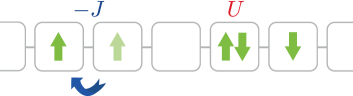
Figure 1: (Color online) Sketch of the one-dimensional Fermi-Hubbard model in real space. Electron hopping is determined by the matrix element $J$, double occupancy of a site costs an additional energy $U$.

To generate a non-equilibrium state a quantum quench is used. Initially, the system is prepared in an eigenstate of $H_{0}$; for simplicity, we use the Fermi sea $\ket{\text{FS}}$. After the quench the time evolution is governed by a different Hamiltonian, i.e., by the full Fermi-Hubbard Hamiltonian $H_{0}+H_{\text{int}}$ including the on-site interaction. Thus, the explicit time dependence of the Hamiltonian is expressed by $H_{\text{Q}}(t)=H_{0}+\theta(t)H_{\text{int}}$ where $\theta(t)$ is the Heaviside function. The state of the system deviates noticeably from $\ket{\text{FS}}$ for times $t>0$. Since the quench in $H_{\text{Q}}(t)$ changes an overall system parameter which influences all sites it is called a global quench. Global quenches are widely considered Manmana et al. (2007); Moeckel and Kehrein (2008, 2009); Manmana et al. (2009); Barmettler et al. (2009); Calabrese, Essler, and Fagotti (2011, 2012a, 2012b); Caux and Essler (2013).

As mentioned in the introduction, we do not exploit or consider the integrability of the above model but use it as simple testbed to illustrate the advocated theoretical approach. Our goal is to compute long-time behavior including infinite-time averages in a systematically controlled way.

III Method

III.1 Dynamics

In order to deduce the time dependence of operators we resort to the iterated equations of motion approach Uhrig (2009); Hamerla and Uhrig (2013a, b, 2014); Kalthoff et al. (2017), a brief summary of which is given in the first part of this section. The second part is dedicated to the necessary modifications of the method which warrant a unitary time evolution on the operator level.

Let us consider an arbitrary operator in the Heisenberg picture

$$A(t)=\sum_{i}h_{i}(t)A_{i}$$ (2)

whose time dependence is completely contained in the complex prefactors $h_{i}(t)$ where the constant operators $A_{i}$ form a suitable operator basis. Throughout this article $\hbar$ is set to unity for simplicity. At this point, only the linear independence of the $A_{i}$ is necessary to make (2) well-defined. Let there be no explicit time dependence of the Hamiltonian such that the Heisenberg equation of motion simplifies to

$$\frac{\text{d}}{\text{d}t}A(t)=i[H(t),A(t)]=:i\mathcal{L}\!\left(A(t)\right)$$ (3)

with the Liouville superoperator $\mathcal{L}\!\left(\cdot\right)$. Inserting (2) into (3) leads to

$$\frac{\text{d}}{\text{d}t}A(t) =i\mathcal{L}\!\left(A(t)\right)$$ (4a)

$$=i\sum_{i}h_{i}(t)\mathcal{L}\!\left(A_{i}\right).$$ (4b)

It is convenient to define linear expansions for all operators $\mathcal{L}\!\left(A_{i}\right)$

$$\mathcal{L}\!\left(A_{i}\right):=\sum_{j}M_{ji}A_{j}$$ (5)

leading to the Liouvillian matrix $\mathbf{M}$, also called dynamic matrix. It is convenient to combine the time dependent prefactors $h_{i}(t)$ to a vector $\mathbf{h}(t)$. Its dynamics is governed by

$$\frac{\text{d}}{\text{d}t}\mathbf{h}(t)=i\mathbf{M}\mathbf{h}(t).$$ (6)

In the Schrödinger picture, the time evolution of the states is determined by the unitary time evolution operator which reads $e^{-iHt}$ for a constant Hamiltonian that has no explicit dependence on $t$. Hence, all solutions are superpositions of oscillatory terms whose frequencies are given by the eigenenergies. Phenomena such as dephasing or relaxation only occur as superpositions of infinitely many terms with continuously distributed frequencies. Mapping the time dependence onto operators and thus switching to the Heisenberg picture does not alter the outcome so that again the temporal evolutions is given by superpositions of oscillatory terms.

Inappropriate approximations, however, will leave us with a dynamic matrix $\mathbf{M}$ which has complex eigenvalues $z_{i}$. Then, exponential behavior arises and if the matrix itself is real the complex eigenvalues occur in pairs $z_{\pm}=R\pm iI$ with real part $R$ and imaginary part $I$. Clearly, one of them induces an exponential divergence in time. Even if the eigenvalues stay real, the matrix may not be diagonalizable, but of Jordan normal form, so that divergences occur which are of power law type. Such divergencies can only be avoided if we can guarantee that $\mathbf{M}$ is diagonalizable with real eigenvalues.

A sufficient, though not necessary, condition to guarantee that $\mathbf{M}$ is diagonalizable with real eigenvalues is to show that it is Hermitian Kalthoff et al. (2017). If $\mathbf{M}=\mathbf{M}^{\dagger}$ is given one knows that the matrix always possesses real-valued eigenvalues $\lambda_{j}$ with equal algebraic and geometric multiplicity such that a general solution to Eq. 6 can always be written as

$$\mathbf{h}(t)=\sum_{j=1}^{f}\alpha_{j}e^{i\lambda_{j}t}\mathbf{v}_{j}$$ (7)

with the corresponding eigenvectors $\mathbf{v}_{j}$ and coefficients $\alpha_{j}$ chosen according to the given initial conditions. Clearly, the general solution is the superposition of oscillatory terms.

How can one be sure that $\mathbf{M}$ is Hermitian in an approximate treatment? In order to compute the matrix easily, it is convenient to use an orthonormal operator basis $\{A_{i}\}$ (ONOB) so that

$$M_{ji}=\left(A_{j}\middle|\mathcal{L}\!\left(A_{i}\right)\right)$$ (8)

holds. Hermitecity of $\mathbf{M}$ means $M_{ji}=M_{ij}^{*}$. It follows from $\mathcal{L}\!\left(\cdot\right)$ being self-adjoint. Whether this is the case or not depends on the choice of the scalar product. Hence, its choice is crucial.

Following Ref. Kalthoff et al., 2017, we define the operator scalar product for two linear operators $A$ and $B$ defined on a Hilbert space $\mathcal{H}$ as

$$\left(A\middle|B\right):=\mathcal{N}\text{Tr}(A^{\dagger}B)~{}\text{with}~{}\mathcal{N}:=\frac{1}{\text{Tr}(\mathbb{1})}.$$ (9)

In so doing, we implicitly assume the (local) Hilbert space to be finite, i.e., $\operatorname{dim}(\mathcal{H})<\infty$. This clearly holds for all spin systems, fermionic systems such as the Fermi-Hubbard model in question, or models with both spin and fermionic degrees of freedom. Bosonic degrees of freedom have to be excluded.

From a physical perspective, the above defined scalar product equals the high-temperature limit $T\to\infty$ of the thermal expectation value

$$\left(A\middle|B\right) =\lim_{T\to\infty}\langle A^{\dagger}B\rangle$$ (10a)

$$=\lim_{T\to\infty}\text{Tr}\left(\rho A^{\dagger}B\right)$$ (10b)

in the canonical ensemble for a density matrix $\rho=\nicefrac{{e^{-\beta H}}}{{Z}}$ with the partition sum $Z=\text{Tr}\left(e^{-\beta H}\right)$, Hamiltonian $H$ and the inverse temperature $\beta\geq 0$. Accordingly, the considered system is maximally disordered and each state of the Hilbert space is equally likely due to $\lim_{T\to\infty}\rho\propto\mathbb{1}$.

The self-adjointness of $\mathcal{L}\!\left(\cdot\right)$ stems from the invariance of the trace under cyclic permutations and allows us to show that $\mathbf{M}$ is Hermitian

$$M_{ji} =\mathcal{N}\text{Tr}(A_{j}^{\dagger}[H,A_{i}])$$ (11a)

$$=\mathcal{N}\text{Tr}(A_{j}^{\dagger}(HA_{i}-A_{i}H))$$ (11b)

$$=\mathcal{N}\text{Tr}([H,A_{j}]^{\dagger}A_{i})$$ (11c)

$$=\left(A_{i}\middle|\mathcal{L}\!\left(A_{j}\right)\right)^{*}$$ (11d)

$$=M_{ij}^{*}.$$ (11e)

Note that there are also other scalar products with the property that the Liouvillian is self-adjoint with respect to them, for instance the expression on the right hand side of (10) at finite temperatures if the ensemble is taken with respect to the Hamiltonian after the quench. But such a scalar product would in practice require detailed knowledge of the Hamiltonian after the quench, for instance its diagonalization. Hence, the choice (9) is very advantageous in the sense that it is easy to use and generally applicable not requiring any particular knowledge of the system. Another asset is that truly time dependent Hamiltonian $H(t)$ with $\partial_{t}H\neq 0$ for almost all times can also be tackled with the choice (9) while more sophisticated choices depending on the actual Hamilton operator would yield time dependent scalar products.

If one follows the advocated strategy it is clear that the time evolution in the Heisenberg picture is unitary in the sense that the operator scalar product remains constant, i.e., for any $A$ and $B$ we have

$$(A(t)|B(t))=(A(0)|B(0)).$$ (12)

This is what is meant by unitarity on the operator level. It can be formally expressed by

$$A(t)=\mathcal{U}(t)A.$$ (13)

implying also that $\langle A(t)\rangle$ consists of the sum of oscillatory terms.

But it does not imply unitarity on the level of states as one knows it from text book quantum mechanics where the unitary solution $U(t)$ of

$$i\frac{\text{d}}{\text{d}t}U(t)=H(t)U(t)$$ (14)

implies that the scalar product of two arbitrary states $\ket{a}$ and $\ket{b}$ stays constant

$$\bra{a(t)}b(t)\rangle =\bra{a(0)}U^{\dagger}(t)U(t)b(0)\rangle$$ (15a)

$$=\bra{a(0)}b(0)\rangle.$$ (15b)

Note that unitarity of the states implies unitarity of operators if we define for any operator $A$

$$\mathcal{U}A:=U^{\dagger}AU.$$ (16)

Then we can conclude

$$(A(t)|B(t)) =\mathcal{N}\text{Tr}(U^{\dagger}A^{\dagger}UU^{\dagger}BU)$$ (17a)

$$=\mathcal{N}\text{Tr}(A^{\dagger}B)$$ (17b)

$$=(A(0)|B(0)).$$ (17c)

The inverse is not true: unitarity on the level of operators does not imply unitarity on the level of states. Inspection of (16) makes this plausible because the left hand side does not impose any particular structure on $\mathcal{U}$ while the right hand side does.

An even clearer piece of evidence results from the inspection of fermionic anticommutators $\{f_{i}^{\dagger},f_{j}^{\vphantom{\dagger}}\}=\delta_{ij}$. Clearly, they stay constant under unitary transformations of the states, i.e., for $f_{i}^{\dagger}(t)=U^{\dagger}f_{i}^{\dagger}U$ and $f_{j}^{\vphantom{\dagger}}(t)=U^{\dagger}f_{j}^{\vphantom{\dagger}}U$ we have

$$\{f_{i}^{\dagger}(t),f_{j}^{\vphantom{\dagger}}(t)\} =U^{\dagger}(f_{i}^{\dagger}UU^{\dagger}f_{j}^{\vphantom{\dagger}}+f_{j}^{\vphantom{\dagger}}UU^{\dagger}f_{i}^{\dagger}\})U$$ (18a)

$$=\delta_{ij}.$$ (18b)

Note that the above identity implies a large number of scalar equations for any given pair $i,j$ because it is an operator identity. For an $F$ dimensional Hilbert space it amounts up to $F^{2}$ scalar equations.

Generically, (18) does not hold for a unitary transformation on the operator level because such a transformation only guarantees the conservation of operator scalar products, i.e., for $f_{i}^{\dagger}(t)=\mathcal{U}f_{i}^{\dagger}$ and $f_{j}^{\vphantom{\dagger}}(t)=\mathcal{U}f_{j}^{\vphantom{\dagger}}$ we have

$$\mathcal{N}\text{Tr}\left(\{f_{i}^{\dagger}(t),f_{j}^{\vphantom{\dagger}}(t)\}\right) =\mathcal{N}\text{Tr}\left(\{f_{i}^{\dagger},f_{j}^{\vphantom{\dagger}}\}\right)$$ (19a)

$$=\delta_{ij}.$$ (19b)

Although the above relation looks similar to (18) it only represents a scalar identity for any given pair $i,j$. In other words, a unitary transformation on operator level is much less restricted than a unitary transformation for states. Still, the unitary time evolution on operator level ensures that the solutions are superpositions of oscillatory terms without any divergencies.

III.2 Time-dependent expectation values

We intend to consider three observables. The first observable is the expectation value of the local particle number

$$n_{i\sigma}(t):=\langle\widehat{n}_{i\sigma}(t)\rangle=\langle\text{FS}|f_{i\sigma}^{\dagger}(t)f_{i\sigma}^{\vphantom{\dagger}}(t)|\text{FS}\rangle$$ (20)

which describes the expectation value of the number of particles present at lattice site $i$ with spin $\sigma$ at time $t$. The expectation value is taken with respect to the ground state of the non-interacting model, i.e., the Fermi sea, because we choose this state as the initial state before the quench.

The second observable is the momentum distribution

$$n_{k\sigma}(t):=\langle\widehat{n}_{k\sigma}(t)\rangle=\langle\text{FS}|f_{k\sigma}^{\dagger}(t)f_{k\sigma}^{\vphantom{\dagger}}(t)|\text{FS}\rangle$$ (21)

where $k$ is the wave vector and $f_{k\sigma}^{\dagger}(t)$ and $f_{k\sigma}^{\vphantom{\dagger}}(t)$ the Fourier transforms of the creation and annihilation operators in real space. Further details are given in Sec. IV.2 where the corresponding results are shown.

The third observable is the jump at the Fermi surface $\Delta n(t)$ defined by

$$\Delta n(t):=\lim_{\mathclap{k\to k_{\text{F}}^{-}}}n_{k\sigma}(t)-\lim_{\mathclap{k\to k_{\text{F}}^{+}}}n_{k\sigma}(t)$$ (22)

for the Fermi wave vector $k_{\text{F}}$. The limits in (22) are meant as one-sided limits and denoted by negative and positive superscripts, respectively.

Since all observables involve one-particle operators they can be easily computed from the time evolution of the elementary fermionic creation and annihilation operators $f_{i\uparrow}^{(\dagger)}(t)$. The most general ansatz reads

$$f_{i\uparrow}^{\dagger}(t)=P_{i}^{\dagger}+\left[P^{\dagger}\left(P^{\dagger}H^{\dagger}\right)\right]_{i}+\ldots$$ (23)

for the creation operator Uhrig (2009); Hamerla and Uhrig (2013a). Here, $P$ stands for a general particle creation operator or a linear superposition of several of them and $(PH)$ stand for a general combination of creation and annihilation operator (hole creation) or a linear superposition of them. The subscript $i$ stands for the site on the lattice around which the operator superposition is located. The terms left out and only indicated by the dots are terms comprising two and more particle-hole pairs.

Concretely, the superposition $P_{i}$ of particle creation operators reads

$$P_{i}^{\dagger}:=\sum_{\delta\lessapprox v_{\mathrm{max}}t}\sum_{\sigma}p_{i\pm\delta,\sigma}^{*}(t)f_{i\pm\delta,\sigma}^{\dagger}$$ (24)

with scalar coefficients $p_{j,\sigma}$. Here, we used that the superposition spreads around its origin at site $i$ only at a finite velocity $v_{\text{max}}$ so that for a given time $t$ significant contributions occur only in a restricted cone $[i-v_{\text{max}}t,i+v_{\text{max}}t]$ according to the Lieb-Robinson bound Lieb and Robinson (1972). Contributions outside of the cone given by the group velocity $v_{\text{max}}$ are exponentially suppressed. If long-ranged interactions are present no such linear cones occur Jurcevic et al. (2014); Hauke and Tagliacozzo (2013); Eisert et al. (2013); Jünemann et al. (2013). But this is not the case we are considering here.

In the following, we use the general representation

$$f_{\ell\uparrow}^{\dagger}=\sum_{m}h^{(\ell)*}_{m}(t)A_{m}^{\dagger}$$ (25)

with $A_{m}$ chosen according to Eq. 23. The superscript indicates the initial lattice site at which the particle is put into the system. Both the occupation number operator and the jump are bilinear expressions in the prefactors $h^{(\ell)}_{n}$. Each term $h^{(\ell)*}_{m}(t)h^{(j)}_{n}(t)$ is multiplied with the expectation value of the corresponding operators, i.e., with

$$A_{mn}=\langle A_{m}^{\dagger}A_{n}\rangle.$$ (26)

These values are taken as matrix elements of the matrix $\mathbf{A}$. Hence, the time dependence of a general bilinear term is given by

$$\langle f_{\ell\sigma}^{\dagger}f_{j\sigma}^{\vphantom{\dagger}}\rangle(t)=\mathbf{h}^{(\ell){\dagger}}(t)\mathbf{A}\mathbf{h}^{(j)}(t).$$ (27)

Note that this evaluation can be numerically demanding because it requires to sum twice over the index of the ONOB. It turns out that often the numerical solution of the differential equations (6) is not the limiting factor, but the actual computation of (27).

The expectation values $A_{mn}$ are computed in the initial state. Hence, it depends on the initial state which values enter and how easy or complicated it is to determine $\mathbf{A}$. In this paper, we choose the Fermi sea as initial state so that the expectation values $A_{mn}$ can be easily computed by factorizing them using Wick’s theorem Wick (1950).

Computing the jump at the Fermi surface requires some additional considerations. Since the Fermi jump is a rescaled Heaviside-like discontinuity it is exclusively determined by terms proportional to $\nicefrac{{1}}{{r}}$, i.e., by terms which have the longest range in real space. A Fourier transform of all these terms yields $\Delta n(t)$. The terms in $\mathbf{A}$ with the longest-range are those which result from the single-particle excitations relative to the Fermi sea Uhrig (2009); Hamerla and Uhrig (2013a). To extract these terms we proceed by normal-ordering the general ansatz (23) for the fermionic creation operator

$$f_{i\uparrow}^{\dagger}(t)=\underbrace{\sum_{m}^{N}H_{m}^{(i)*}(t)\,{:}\mkern 0.4muf_{m\uparrow}^{\dagger}\mkern 0.6mu{:}}_{\begin{subarray}{c}\text{one-particle}\\ \text{contributions}\end{subarray}}+{:}\mkern 0.4mu\left[P^{\dagger}\left(P^{\dagger}H^{\dagger}\right)\right]_{i}\!\mkern 0.6mu{:}\,+\ldots\ .$$ (28)

Only the first term relates to single-particle excitations and thus matters for the jump $\Delta n$. Here, additional superscripts clarify which initial conditions are used, i.e., they are used to denote the lattice site at which a particle is inserted at time $t=0$. For general observables superscripts are omitted for brevity.

We highlight that the approach advocated here consists of two steps, in contrast to what has been realized previously Hamerla and Uhrig (2013a, b, 2014). In the first step, an ONOB is used to describe the evolution of operators in the Heisenberg picture. No normal-ordering enters at this stage differing from what has been done before. Only in the second step, we normal-order the operators of the ONOB in order to distill the single-particle part relevant for the jump at the Fermi level.

The concrete procedure runs as follows. Consider the annihilation operator and let

$$H^{(0)}_{n}(t)=\sum_{j}t_{nj}h^{(0)}_{j}(t)$$ (29)

where $h^{(0)}_{j}(t)$ is the time-dependent prefactor of the operator $A_{j}$ and $t_{nj}\in\mathbb{C}$ quantifies to which extent the normal-ordering of the operator $A_{j}$ contributes to the single-particle operator $f_{n\sigma}^{\vphantom{\dagger}}={:}\mkern 0.4muf_{n\sigma}^{\vphantom{\dagger}}\mkern 0.6mu{:}$, see also (28). Hence, the factors $t_{nj}$ are two-point expectation values or sums of products of them according to Wick’s theorem. For instance, $t_{5j}=2^{3/2}\langle n_{3}-1/2\rangle$ if $A_{j}=2^{3/2}f_{5\uparrow}^{\vphantom{\dagger}}(f_{3\downarrow}^{\dagger}f_{3\downarrow}^{\vphantom{\dagger}}-1/2)$. Hence, the coefficients $t_{nj}$ represent the effect of normal-ordering, given that an arbitrary operator basis has been chosen before.

It is an advantage of the Fermi jump that it can be computed from the coefficients $H_{n}$. Each of these coefficients requires only a single sum over the ONOB whereas other observables require a double sum over the ONOB which is of large dimensionality. We once again stress that the actual integration of the differential equation (6) does not represent the bottleneck generically, but the final evaluation of the expression (27).

Once the one-particle prefactors $H_{n}(t)$ are determined, the jump $\Delta n(t)$ can be computed either by

$$\Delta n(t)=\sum_{m,n}^{N}H^{(0)*}_{m}(t)H^{(0)}_{n}(t)e^{ik_{\mathrm{F}}(m-n)}$$ (30)

or by first computing the Fourier series Uhrig (2009); Hamerla and Uhrig (2013a, b)

$$H^{(0)}_{k}(t) =\sum_{n}H^{(0)}_{n}(t)\exp(-ikn)$$ (31a)

and then taking the square of its absolute value

$$\Delta n(t) =|H^{(0)}_{k}(t)|^{2}.$$ (31b)

III.3 Infinite-time averages

We focus here on the temporal evoluation for long times in particular. The long-term behavior of observables contains information about whether and to which extent a quenched system retains information about its initial state. Moreover, it provides evidence if and how the system approaches stationary states. In particular, the averages over infinitely long time intervals provide information about the expectation values of the stationary state.

In this section we analytically derive such averages for observables. While many approaches require to numerically compute the temporal evolution in order to finally average over it our method directly addresses the averaged quantities. The observable average for $t\to\infty$ can be computed based on the knowledge of the initial correlation at time $t=0$ without the calculation of any time dependence. Of course, it is also possible to average a computed temporal evolution over suitably chosen time intervals, for instance in order to address the same quantities as measured in experiment.

We define the infinite-time average of an observable by

$$O_{\infty}:=\lim_{t\to\infty}\frac{1}{t}\int_{0}^{t}\text{d}t^{\prime}\langle O(t^{\prime})\rangle.$$ (32)

This definition is particularly helpful in situations without a well-defined infinite-time limit $\lim_{t\to\infty}\langle O(t)\rangle$ due to non-vanishing oscillatory contributions. Calculating the infinite-term average (32) can be performed in a fully analytical approach provided that the constraints of Sec. III.1 are met.

Due to the equality of Heisenberg and Schrödinger picture at $t=0$ the prefactors $\alpha_{j}$ in (7) are determined. For simplicity, we include these initial conditions in scaled eigenvectors by defining

$$\mathbf{\overline{v}}_{j}:=\alpha_{j}\mathbf{v}_{j}.$$ (33)

Note that only the $\alpha_{j}$ depend on different initial conditions. In the following, $\overline{v}_{p,q}$ denotes the $q$-th component of the scaled eigenvector $\mathbf{\overline{v}}_{p}$ and thus describes the contribution to $h_{q}(t)$ in Eq. 2.

Inspecting the temporal evolution of the prefactors $\mathbf{h}(t)$ in (7) the oscillatory contributions are shown to vanish in the infinite-time averages which implies that only the terms with stationary phases contribute to them Fioretto and Mussardo (2010). For the infinite-time average we obtain

$$\lim_{t\to\infty}\frac{1}{t}\int_{0}^{t}\text{d}t^{\prime}h^{*}_{m}(t^{\prime})h_{n}(t^{\prime})$$ (34a)

$$=\sum_{i,j}\overline{v}_{i,m}^{\,*}\overline{v}_{j,n}\underbrace{\lim_{t\to\infty}\frac{1}{t}\int_{0}^{t}\text{d}t^{\prime}e^{i(\lambda_{j}-\lambda_{i})t^{\prime}}}_{=\,\delta_{\lambda_{i},\lambda_{j}}}$$ (34b)

$$=\sum_{\begin{subarray}{c}i,j\\ \lambda_{i}=\lambda_{j}\end{subarray}}\overline{v}_{i,m}^{\,*}\overline{v}_{j,n}.$$ (34c)

Consequently, only contributions located within the same subspace spanned by the eigenvectors of the same eigenvalue do not vanish in the long run.

Applying (34) to the infinite-time average of the local particle number operator the following relation holds

$$n_{\infty} =\lim_{t\to\infty}\frac{1}{t}\int_{0}^{t}\text{d}t^{\prime}\sum_{m,n}h^{(0)*}_{m}(t^{\prime})h^{(0)}_{n}(t^{\prime})\langle A_{m}^{\dagger}A_{n}\rangle$$ (35a)

$$=\sum_{\begin{subarray}{c}i,j\\ \lambda_{i}=\lambda_{j}\end{subarray}}{\vphantom{\overline{\mathbf{v}}}}\overline{\mathbf{v}}^{(0)\dagger}_{i}\mathbf{A}\overline{\mathbf{v}}^{(0)}_{j}$$ (35b)

where we used the expectation value matrix $\mathbf{A}$ defined by its matrix elements in (26).

Finally, we turn to the Fermi jump. Its general time dependence is given by Eq. 30. Averaging over infinite time using (34) we obtain

$$\lim_{t\to\infty}\int_{0}^{t}\text{d}t^{\prime}H_{m}^{(0)*}(t^{\prime})H_{n}^{(0)\vphantom{*}}(t^{\prime})$$ (36a)

$$=\sum_{p,q}t_{mp}^{*}\,t_{nq}^{\vphantom{*}}\lim_{t\to\infty}\int_{0}^{t}\text{d}t^{\prime}h_{p}^{(0)*}(t^{\prime})h_{q}^{(0)}(t^{\prime})$$ (36b)

$$=\sum_{\mathclap{\begin{subarray}{c}p,q,i,j\\ \lambda_{i}=\lambda_{j}\end{subarray}}}t_{mp}^{*}t_{nq}^{\vphantom{*}}\overline{v}_{i,p}^{(0)*}\overline{v}_{j,q}^{(0)}$$ (36c)

$$=\sum_{\mathclap{\begin{subarray}{c}i,j\\ \lambda_{i}=\lambda_{j}\end{subarray}}}{\vphantom{\overline{\mathbf{v}}}}\overline{\mathbf{v}}^{(0)\dagger}_{i}\mathbf{T^{mn}}\overline{\mathbf{v}}^{(0)}_{j}$$ (36d)

with the usually highly sparse transformation matrix $\mathbf{T^{mn}}$ defined by its matrix elements

$$T_{pq}^{mn}:=t_{mp}^{*}t_{nq}^{\vphantom{*}}.$$ (37)

Consequently, the infinite-time average of the jump can be expressed very concisely by

$$\Delta n_{\infty}=\sum_{m,n}^{N}\sum_{\mathclap{\begin{subarray}{c}i,j\\ \lambda_{i}=\lambda_{j}\end{subarray}}}{\vphantom{\overline{\mathbf{v}}}}\overline{\mathbf{v}}^{(0)\dagger}_{i}\mathbf{T^{mn}}\overline{\mathbf{v}}^{(0)}_{j}\,e^{ik_{\mathrm{F}}(m-n)}.$$ (38)

This concludes the general part of the advocated approach. We stress again, that the above method allows us to address directly the expectation values of the stationary state assumed at infinite times.

III.4 Lanczos algorithm

The calculations in Sec. III.3 are analytical ones, but their evaluation finally involves numerics. Thus, it is instructive to discuss numerical implications. For the infinite-time averages eigenvalues and eigenvectors are needed so that a full diagonalization of the Liouville matrix is required. Its run time scales like $\mathcal{O}\left(F^{3}\right)$ where $F$ is the dimension of the ONOB. This may become a very large number so reductions of the matrix dimensions are of interest. An efficient technique for achieving this goal must eliminate less needed directions leading to a reduced matrix $\mathbf{\widetilde{M}}\in\mathbb{C}^{f\times f}~{}\text{with}~{}f<F$ with modified eigenvectors which span a smaller subspace $\widetilde{S}$ than the original $S=\mathrm{span}\left(\left\{\mathbf{v}_{j}\right\}\right)$.

Accordingly, not all former vectors $\mathbf{r}\in S$ are still element of $\widetilde{S}$. In order to fulfill the initial condition truncation has to ensure that $\mathbf{h}(0)\in\widetilde{S}$ holds. The Lanczos algorithm Lanczos (1938) fulfills these requirements. It is a special case of the Arnoldi iteration Arnoldi (1951) for Hermitian matrices. Starting from the initial condition vector $\mathbf{s}:=\mathbf{h}(0)$ it gradually constructs the $f$-dimensional Krylov space of operators

$$\mathcal{K}^{f}\!\left(\mathbf{s}\right)=\mathrm{span}\left(\mathbf{s},\,\mathbf{M}\mathbf{s},\,\mathbf{M}^{2}\mathbf{s},\ldots,\,\mathbf{M}^{f-1}\mathbf{s}\right).$$ (39)

The time required to diagonalize the smaller tridiagonal Liouville matrix $\mathbf{\widetilde{M}}$ in this Krylov space can be significantly reduced. The precise gain in run time depends on the ratio of $f$ to $F$.

III.5 Operator monomials

For arbitrary $0<\nicefrac{{J}}{{U}}<\infty$ each application of the Liouville operator, i.e., each commutation with $H$, is prone to create operator monomials which were not yet in the considered basis. In the following discussion all time-dependent prefactors are omitted for brevity, but one should keep in mind that each operator monomial comprises also such a prefactor. The shorthand $\mathcal{L}_{p}\!\left(\cdot\right)$ stands for a commutation with $H_{p}$ where $p=0$ or $p=\text{int}$. The set of lattice sites in real space where an operator monomial has a non-trivial effect, i.e., has a local operator different from the identity, is called the corresponding cluster. Often, the terms “operator monomial” and “cluster” are used interchangeably if one focusses on the relevant sites.

Fig. 2 graphically illustrates the effects of both hopping and interaction on operator monomials. The hopping part $H_{0}$ moves operators through the lattice and the interaction part generates monomials with increasing numbers of operators. Consequently, no finite operator basis is closed under iterated commutation with $H_{0}$ and $H_{\text{int}}$. Generically, the number of sites involved proliferates upon commutation, i.e., the clusters continuously grow.

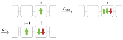
Figure 2: (Color online) Combined effect of hopping and interaction: Green (red) colored arrows stand for particle (hole) creation operators, the spin direction is described by the arrow orientation.

Not all operators contribute to the dynamics to the same extent depending on the parameter regime. Exemplarily, for the limit of strong on-site repulsion, i.e., $\nicefrac{{J}}{{U}}\ll 1$, hopping represents a small perturbation and plays a minor role since nearly local processes dominate the time evolution of the system. We focus on this particular regime and refrain from including physically strongly suppressed operators in the ONOB. This means that monomials generated by many hopping processes are neglected.

Periodic boundary conditions for a lattice of $N$ sites are used. We choose a fixed ONOB constructed with respect to locality and orthonormality in the sense of the scalar product (9). We start from local creation operators, apply the Liouville operator and project the resulting expression onto the subspace spanned by operators in the chosen ONOB. Roughly, a larger ONOB with more operators is expected to provide better results Kalthoff et al. (2017).

Concretely, we apply $\mathcal{L}_{0}\!\left(f_{i\uparrow}^{\dagger}\right)\propto f_{i\pm 1\uparrow}^{\dagger}$ and $\mathcal{L}_{\mathrm{int}}\!\left(f_{i\uparrow}^{\dagger}\right)\propto f_{i\uparrow}^{\dagger}f_{i\downarrow}^{\dagger}f_{i\downarrow}^{\vphantom{\dagger}}$ and orthonormalize the resulting operators which yields

$$w_{1}^{\dagger}(i) =\sqrt{2}f_{i\uparrow}^{\dagger}$$ (40a)

$$w_{2}^{\dagger}(i,j,k) =\left(\!\sqrt{2}\right)^{3}f_{i\uparrow}^{\dagger}\left(f_{j\downarrow}^{\dagger}f_{k\downarrow}^{\vphantom{\dagger}}-\frac{1}{2}\delta_{jk}\right).$$ (40b)

These two operator families comprise $N^{3}+N$ operators in total. Since the corresponding cluster consists of at most three distinct lattice sites we call the ONOB given in Eq. 40 the $3$-basis. We stress that the $3$-basis is invariant under repeated application of $\mathcal{L}_{0}\!\left(\cdot\right)$, i.e., the application $\mathcal{L}_{0}\!\left(\cdot\right)$ does not lead to operators which are not linear combinations of operators in the $3$-basis. It allows us to reach the same level of description which was reached perturbatively by continuous unitary transformations Moeckel and Kehrein (2008, 2009).

We use the $3$-basis as a suitable starting point. Next, we modify it to be invariant under the application of $\mathcal{L}_{\mathrm{int}}\!\left(\cdot\right)$ because we aim here at a description of strong interaction quenches where the local terms dominate. Since the local Hilbert space is four dimensional, there are at most 15 non-trivial local operators. Due to the symmetries of the Hamiltonian such as particle number and spin conservation we only need seven additional operator families with up to nine fermionic creation and annihilation operators each, see Appendix A, in order to extend the $3$-basis to the $3^{+}$-basis which is closed under application of $\mathcal{L}_{\mathrm{int}}\!\left(\cdot\right)$. The $3^{+}$-basis is well suited for strong quenches where hopping can be seen as a pertubation. The basis is exact up to monomials of order $\left(\nicefrac{{J}}{{U}}\right)^{2}$ because it comprises up to three sites and, starting from a single sites, clusters of three sites require at least two hopping processes.

IV Observables

IV.1 Occupation number operator

The local particle number $n_{i\sigma}(t)$ and its infinite-time average are the first quantities we address. Of course, particle-conservation in a translational invariant system tells us that these quantities have to be constant in time and equal to the filling factor $n$. But the advocated approach does not imply this automatically so that the proper non-dependence on time provides a perfect first test for the accuracy of the approach. Any deviations of $n_{i\sigma}(t)$ from $n$ can be ascribed to approximations induced by the finite bases. In this way, we can also assess the different performances of the $3$-basis and the $3^{+}$-basis.

Due to translational invariance the considered lattice site is arbitrary and will be fixed to $i=0$ from now on. The time evolution of the particle number operator is thus calculated using

$$n_{0\uparrow}(t)=\langle\widehat{n}_{0\uparrow}(t)\rangle=\sum_{m,n}h^{(0)*}_{m}(t)h^{(0)}_{n}(t)\langle A_{m}^{\dagger}A_{n}\rangle.$$ (41)

For the infinite-time average we employ the analytical approach (35).

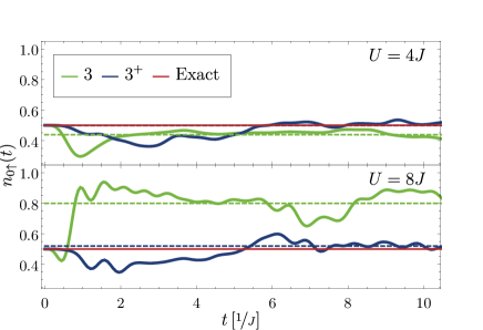
Figure 3: (Color online) Local particle number computed for the $3$-basis and the $3^{+}$-basis, for two interaction strengths $U$ at half-filling $n=1/2$. The horizontal dashed infinite-time averages $n_{\infty}$ are depicted for orientation.

Fig. 3 compares results from the two ONOBs used. Two qualitatively distinct parameter regimes are studied. For the regime $U=W=4J$ the physical effects of hopping and on-site interaction balance each other which is why the $3^{+}$-basis and the $3$-basis are expected to lead to qualitatively similar results. This agrees with the calculated results. We stress, however, that the semi-analytically computed infinite-time average $n_{\infty}$ of the $3^{+}$-basis is noticeably closer to the exact filling $n=1/2$ than the equivalent average of the $3$-basis.

Results for the second parameter regime $U=8J$ with a dominating on-site repulsion agree as well with the expectations. Operator monomials created by application of $\mathcal{L}_{\text{int}}\!\left(\cdot\right)$ gradually gain more weight for $\nicefrac{{J}}{{U}}\to 0$. Thus, the $3^{+}$-basis is describing the true expectation value of the local particle number significantly better. We again emphasize that the inserted infinite-time averages (horizontal dashed lines) are not calculated by averaging numerically over $n_{0\uparrow}(t)$ for some time interval. Instead, they fully rely on the Liouville matrix and the initial condition at $t=0$. We checked that $n_{\infty}$ agrees with the corresponding time averages over $n_{0\uparrow}(t)$ for sufficiently long, but finite times (not shown here).

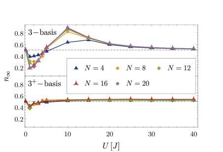
Figure 4: (Color online) Infinite-time averages $n_{\infty}$ for the $3$-basis and $3^{+}$-basis depending on $U$. The dashed black lines denote the analytically correct result for half-filling. Especially the $3^{+}$-basis is able to keep this value regardless of $U$ except for a dip around $U\approx J$ while the $3$-basis appears not to be very reliable. Calculations in the upper (or lower) panel are computed using the Lanczos algorithm for a maximum Krylov space dimension $f$ of a third of the overall Hilbert space dimension (or $f\leq 1000$). A lattice size of $N=20$ was examined for the $3$-basis only.

To examine the two ONOBs further the infinite-time average $n_{\infty}$ in dependence of $U$ is displayed in Fig. 4. We highlight that especially in the range of $U\approx 10J$ the $3^{+}$-basis is considerably superior to the $3$-basis regarding the long-term accuracy.

We conclude that the advocated approach works well. It is systematically controlled such that the larger operator basis provides better results. For the Hubbard model under study the $3^{+}$-basis is a very good choice which we will employ in the remainder of this article for this reason. The high accuracy of the directly accessible infinite-time averages, cf. Fig. 4, is very promising, in particular for relatively strong interaction quenches.

IV.2 Momentum distribution

The momentum distribution is a key quantity in solid state physics and for artificial systems of ultracold atoms in optical lattices. It can be considered in equilibrium and out-of-equilibrium. In solid state systems, angular-resolved photoemission spectroscopy is a tool to measure momentum dependencies Damascelli, Shen, and Hussain (2003). But the determination of the momentum distribution remains difficult because matrix element effects play an important role and they are not easy to capture quantitatively.

The measurement of momentum distributions in systems of optical lattices is relatively easy. At each desired instant of time the optical lattice and any trapping potential is switched off suddenly so that the particle spread according to their instant velocities $\mathbf{v}\propto\mathbf{k}$. Hence, after a certain delay time an image of the particle distribution reveals the momentum distribution just before the sudden release Bloch, Dalibard, and Zwerger (2008). Due to its importance we address the time-dependent momentum distribution here.

Using the time-dependent non-local correlations

$$g_{l\sigma}(t):=\langle\text{FS}|f_{0\sigma}^{\dagger}(t)f_{l\sigma}^{\vphantom{\dagger}}(t)|\text{FS}\rangle$$ (42)

with their initial values for the Fermi sea for a finite lattice with periodic boundary conditions of $N$ sites

$$g_{l\sigma}(t\!=\!0)=\frac{1}{N}\sum_{\mathclap{|k|\leq k_{\mathrm{F}}}}e^{ikl}$$ (43)

the time-dependent number of particles with momentum $k$ and spin $\sigma$ for time $t$ reads

$$n_{k\sigma}(t)=\frac{1}{N}\sum_{l}e^{-ikl}g_{l\sigma}(t)$$ (44)

in the one-dimensional model under consideration. The results of the momentum distribution for the $3^{+}$-basis are shown in Figs. 5 and 6.

Figure 5: (Color online) Momentum distribution for a lattice of $N=12$ sites after being quenched to $U=4J$ vs. time. Only the range of $k\in[0,\pi]$ (lattice constant is set to unity) is shown due to symmetry. Finite-size features are the washed-out transition between occupied and unoccupied states at $t=0$. Starting from the Fermi sea an out-of-phase oscillation of the initially occupied and unoccupied states occur with almost featureless distributions in between.

Figure 6: (Color online) Momentum distribution for a lattice of $N=12$ sites after being quenched to $U=20J$ vs. time. Qualitatively, the same behavior as in Fig. 5 can be observed. Compared to results of $U=4J$ the time period of the oscillations is much shorter and there is a huge increase in their amplitudes. At about $t\approx 1.7J^{-1}<t_{\mathrm{WA}}$ a dip in the momentum distribution for excitations of long wavelengths, i.e., $k\approx 0$, is visible.

The quench to $U=4J$ is found to be in good agreement with data from an iterated equations of motion approach without a unitarity preserving scalar product Hamerla and Uhrig (2013b); Hamerla (2013) for times up to which the reference results are converged, i.e., $t\lessapprox 1J^{-1}$. Note that these reference data can be regarded as exact up to the time threshold up to which they are converged. Our data, however, can be trusted up to significantly longer times. For the strong quench regime of $U=20J$ there is no data available for comparison.

There are two main reasons for deviations of our results from the true thermodynamic behavior. The first one is the use of a truncated basis as discussed in detail above. In the present work, the truncation is systematically controlled by the choice of the $3^{+}$-basis which is exact up to and including order $(J/U)^{2}$. The second reason is the evaluation of the dynamics on finite chains. This implies that wrap-around effects are possible. An operator at site 0 will propagate along the chain till it reaches its maximum distance at site $N/2$ after a time $t_{\mathrm{WA}}$. A complete wrap-around occurs after time $t=2t_{\mathrm{WA}}$.

To assess the reliability of our approach we estimate the maximum speed $v_{\mathrm{max}}$, with which information can travel Lieb and Robinson (1972), cf. Sec. IV.3, by the Fermi velocity $v_{\mathrm{F}}=\left.\frac{\text{d}}{\text{d}k}\epsilon_{k}\right|_{k=k_{\mathrm{F}}}$ of the non-interacting model. We assume that this estimate rather overestimates $v_{\mathrm{max}}$ because the true velocities in the interacting Hubbard model are generically smaller due to dressing effects. At half-filling, $v_{\mathrm{F}}=2J$ for the lattice constant set to unity. Hence we arrive at

$$t_{\mathrm{WA}}\approx\frac{N}{4}J^{-1}$$ (45)

for the time to reach the maximum distance from the initial site on a ring.

Consequently, our results for the momentum distribution in Figs. 5 and 6 are taken to be correct up to at least $t_{\mathrm{WA}}=3J^{-1}$ for the finite lattice size $N=12$ considered. Still, we are able to study the momentum distribution in this way for a significantly longer time span than previous similar studies Hamerla and Uhrig (2013a, b). We will see below, that noticeable wrap-around effects only occur at about $2t_{\mathrm{WA}}$ with $t_{\mathrm{WA}}$ from (45).

The moderate quench to $U=4J=W$ and the strong quench to $U=20J=5W$ both lead to a considerable redistribution of occupied momenta. The initial state is the Fermi sea with clearly occupied and empty momenta. This distribution is followed directly after the quench by a rapid increase (decrease) of the average occupation number for $|k|>k_{\mathrm{F}}$ ($|k|<k_{\mathrm{F}}$) with Fermi momentum $k_{\mathrm{F}}=\nicefrac{{\pi}}{{2}}$. After this transient rapid change of the occupation of the momenta the regions separated by $k_{\mathrm{F}}$ oscillate out-of-phase with an average oscillation period $T$. Dedicated analysis, see below, shows that especially in the strong quench regime the dominant oscillation possesses a period $T$ of about

$$T=\frac{2\pi}{U}.$$ (46)

The physical interpretation is straightforward. In the limit $\nicefrac{{J}}{{U}}\to 0$ the Fermi-Hubbard model is mainly governed by local processes which induce Rabi oscillations between singly and doubly occupied sites with periods according to (46) because their energy difference is $U$ Hamerla and Uhrig (2013a, b, 2014). This is analogous to spin precession about the $z$-axis if initially the spin points along a transversal direction in the $xy$-plane. In the quenches, the initial state is a superposition of the two local possibilities of singly and doubly occupied sites. Note that at half-filling both, single occupation and double occupation, are two-fold degenerate. Single occupation due to the two spin states and double occupation because the completely empty site acts like a site doubly occupied with holes.

The Rabi oscillations do not die out, but persist on the accessible time scales. The momentum distribution for $t<t_{\mathrm{WA}}$ shows a nearly periodic behavior with little changes in amplitude and frequencies. This seems to hint at a (quasi-)stationary state of a constant momentum distribution being overlaid by oscillations. At present, it is not clear whether the oscillations decay for $t\to\infty$ and in which way the amplitude of the oscillations depend on the system size. Further investigations of the time-dependent momentum distribution are called for. For the jump at the Fermi surface, we address these issues below.

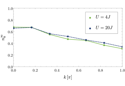
Figure 7: (Color online) Infinite-time average of the momentum distribution $n_{k}^{\infty}$ for two different values of $U$ for a periodic chain of $N=12$ sites. The infinite-time averaged distributions are very similar and featureless. They show comparatively highly occupied momenta for $k>\frac{\pi}{2}$ which were initially completely empty. This calculation is based on a complete diagonalization and does not make use of the Lanczos algorithm.

To further assess the character of the stationary state in question we apply the concept of infinite-time averages to the momentum distribution. The explicit expression reads

$$g_{l\sigma}^{\infty}=\sum_{\begin{subarray}{c}i,j\\ \lambda_{i}=\lambda_{j}\end{subarray}}{\vphantom{\overline{\mathbf{v}}}}\overline{\mathbf{v}}^{(0)\dagger}_{i}\mathbf{A}\overline{\mathbf{v}}^{(l)}_{j}$$ (47)

for the real space correlations. The momentum distributions ensue by computing the Fourier series of the $N$ correlation functions (47). Note that Eq. 47 is merely a generalization of Eq. 35. Consequently, only an adjustment of the initial conditions for the annihilation operator is needed. This is what the additional superscripts indicate, cf. Sec. III.3.

Results of this approach are shown in Fig. 7. Only a slight decrease of the average occupation number for increasing momenta is visible. Otherwise the infinite-time momentum distribution is remarkably featureless. Note that both quenches, the moderate one to $U=4J$ and the strong one to $U=20J$, result in very much the same momentum distribution. The results shown are obtained for a finite chain of $12$ sites. The computation is fairly demanding due to the large dimension of the operator basis. Calculation in the thermodynamic limit based on an operator basis truncated by a finite range of the operator clusters is an interesting step to be tackled next.

IV.3 Evolution of the jump at the Fermi surface

The striking characteristics of the initial Fermi sea is the discontinuity at the Fermi wave vector $k_{\mathrm{F}}$. Hence, we track the temporal evolution of this jump after the quench quantitatively in order to learn more about oscillations at finite times, the stationary state for infinite times, and how the latter is approached.

In a direct calculation on finite lattices the jump is not accessible because the one-sided limits cannot be computed. Thus we use the elegant detour via the one-particle contributions $H_{n}(t)$ yielding the Eq. 30.

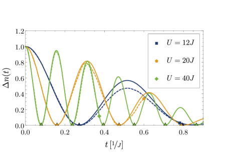
Figure 8: (Color online) Comparison of results obtained using the scalar product for operators (solid lines) and results calculated for normal-ordered operators without scalar product Hamerla and Uhrig (2013b); Hamerla (2013) (dashed lines). The latter results are calculated in a highly accurate approach, but are only converged up to short times. The respective maximum times are given by the three different plot symbols. Triangles at the $x$-axis mark predictions for zeros of the curve based on the Rabi oscillations (46).

For a comparison of results of the iterated equations of motion approach using the scalar product given in Eq. 9 and not using it Hamerla and Uhrig (2013a, b); Hamerla (2013); Hamerla and Uhrig (2014) we display Fig. 8. The data depicted by the dashed curves is highly accurate where it is converged, i.e., for short time spans only. The time range shown and used for comparison is adapted accordingly.

Two striking phenomena are to be observed. First, for all interaction strengths the zeros of each curve agree for both methods extremely well. In the considered regime of quenches to strong interactions we see that the simple estimate for the period of the observed Rabi oscillations (46) matches the zeros very well, see the triangular symbols at the bottom axis. The first symbol is put at the first zero of the computed curves; the following symbols are placed at multiples of the Rabi period $T$. Prediction and actual data agree remarkably well.

Second, the amplitudes for both approaches nearly coincide for $U\geq 20J$. This shows that the scalar product method yields accurate results in the limit of strong quenches. This provides two advantages: (i) the operator basis to be considered, though large, is much smaller in the present approach than in the previous approach. (ii) The present approach is able to capture noticeably longer time spans so that it renders more extensive examinations possible, for instance addressing relaxation behavior.

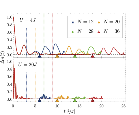
Figure 9: (Color online) Jump at the Fermi surface for two values of $U$ (upper/lower panel) in dependence on the lattice size $N$. Finite-size revivals occur the earlier the smaller the lattice is. Once a finite-size revival has occurred the data is cropped by hand. The corresponding end-of-curve is denoted by the four different glyphs. Dashed vertical lines mark $t_{\mathrm{WA}}$, i.e., the time up to which results are estimated to be independent of $N$, colored triangles mark the instants $2t_{\mathrm{WA}}$ which indeed almost coincide with the onset of the spurious finite-size revivals.

For an in-depth analysis of the impact of finite-size effects on the results we calculate the jumps at the Fermi surface for different lattice sizes $N$. The results are shown in Fig. 9. The initial evolutions of the jump are identical for all sizes. The jump starts at its maximum value of unity and decreases very briefly thereafter in an oscillatory manner. We see a collapse-and-revival phenomenon as has been observed beforeHamerla and Uhrig (2014) until the jump vanishes completely.

Upon increasing $N$ the finite-size revivals occur later and later. The time instant at which these spurious features set in is estimated very well by $2t_{\mathrm{WA}}$, see triangles at the bottom of both panels in Fig. 9. For sufficiently large $N$, the jump has essentially vanished before any finite-size effect sets in.

Interestingly, the evolution up to $2t_{\mathrm{WA}}$ is almost independent of the system size. This observation is very promising because it implies that we are able to capture the essential dynamics of the Fermi jump by considering finite systems. This allows for a reduction of numerical effort in future studies for cases where the behavior up to specific times is needed only.

We conclude from Fig. 9 that the jump of the Fermi surfaces vanishes very quickly. One is tempted to conclude that the system relaxes on these short time scales. But inspection of Figs. 5 and 6 reveals that significant oscillations still take place at momenta far away from the Fermi wave vector $k_{\mathrm{F}}$ when the Fermi jump has already disappeared. Hence, further studies of these oscillations and their dependence on time, interaction, and system size is necessary, but left for future research.

Investigating Fig. 9 we see that the decaying oscillations are governed by more than one single frequency. In particular in the lower panel displaying data for a quench to $U=20J$ one discerns a beating in the oscillations with a zero amplitude at about $t\approx 1.2/J$. This is a clear indication of the presence of at least two frequencies. To analyze the relevant frequencies in the evolution of the Fermi jump systematically we use Fourier analysis. But it is hampered by the discontinuous onset at $t=0$ where the signal starts. Since we want to focus only on the frequency content we transform the symmetrized signal $\Delta n(t)+\Delta n(-t)$, which we additionally smoothen by means of a low-pass Gaussian filter, by fast Fourier transform.

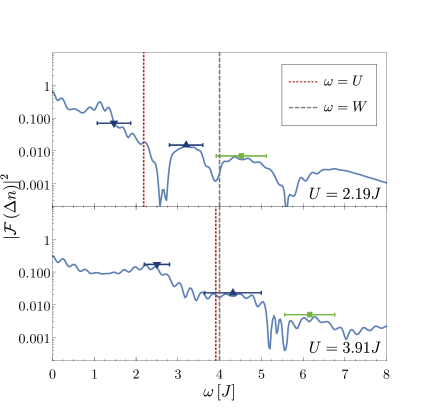
Figure 10: (Color online) Spectra as obtained by Fourier transform from the time-dependent symmetrized Fermi jump for weaker interaction quenches. The symbols with error bars indicate spectral features which we read off.

Figs. 10 and 11 display the squares of the absolute values of the resulting spectra for various quenches in logarithmic plots. The value of the quenched interaction is indicated in the panels. The colored symbols with error bars show the frequencies which we read off. Mostly they indicated peaks, but also shoulders, see the low-frequency feature in the upper panel of Fig. 10. We choose to read off this feature because at even smaller interaction only the shoulder can be identified.

The vertical dashed lines show two typical energies of the system, namely the band width $W$ and the interaction strength $U$ for orientation and comparison. It appears that both of them show up in the spectral features, i.e., spectral features occur at frequencies which are close to $W$ or $U$.

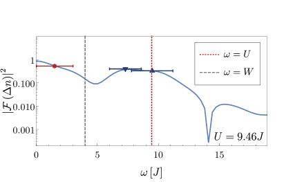
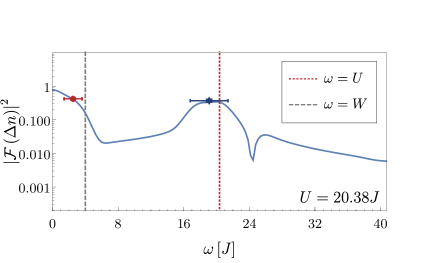
Figure 11: (Color online) Spectra as obtained by Fourier transform from the time-dependent symmetrized Fermi jump for stronger interaction quenches. The symbols with error bars indicate spectral features which we read off.

Note that different symbols are chosen to display different spectral structures. Upon increasing $U$, the high-frequency feature shown using a green square shifts to higher and higher values, but becomes less and less significant, see also Fig. 11. Beyond a certain value of $U$ it does not appear anymore. In parallel, a low-frequency feature appears which was not discernible before. We denote it by the red hexagons in Fig. 11. Comparing the upper and the lower panel of Fig. 11 it appears that the two peaks indicated by blue triangles, which are still discernible in the upper panel, are merged in the lower panel. So they are denoted by a single symbol formed from both triangles.

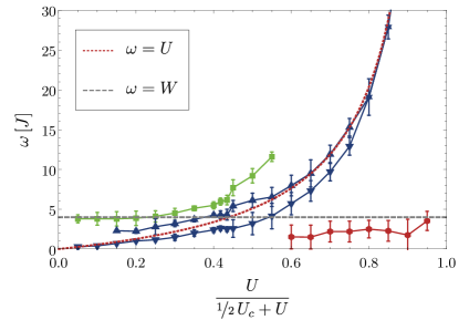
Figure 12: (Color online) Frequencies of the most important spectral features in the spectra of $\Delta n(t)$ plotted as functions of the interaction strength. The latter is given in a compactified form with $U_{c}=-8E_{\mathrm{kin}}/N$ where $E_{\mathrm{kin}}/N=-W/\pi$ is the kinetic energy per site of the half-filled non-interacting system. This allows us to show the full range from $U=0$ to $U=\infty$. The error bars are determined approximately by the half-widths at half maximum of the peaks. The frequency of local Rabi oscillations, i.e., $\omega=U$, and the band width, i.e., $\omega=W$, are depicted for comparison as dashed lines.

We analyzed many more spectra than the four shown here explicitly. The data is compiled in Fig. 12. In total, we identified four relevant spectral features. At weak quenches there is clearly one feature given by the band width $W$, shown by the green curve in Fig. 12. Besides this feature, there are two features located at frequencies above and below the local Rabi frequency $U$ (blue curves). The lower frequency almost coincides with $U$ for weak quenches. We stress that the features for weak quenches must be regarded with some caution because the choice of the ONOB is designed for strong quenches.

For strong quenches, there occurs a low-frequency feature depicted by the red curve. It does not coincide quantitatively with the band width $W$, but it is close to it within a factor of two. Given the difficulty to extract the proper frequency for the low-frequency feature, see Fig. 11, the quantitative deviations are not surprising. The high-frequency feature clearly matches the local Rabi frequency $U$ almost quantitatively. The two spectral feature above and below $U$ merge for larger $U$, at least they can no longer be detected separately, see lower panel of Fig. 11.

The intermediate parameter region $U\approx U_{c}/2$ in Fig. 12 is of particular interest. In previous analyses Eckstein, Kollar, and Werner (2009); Schiró and Fabrizio (2010, 2011); Hamerla and Uhrig (2013a) it seemed as if there were two qualitatively distinct regimes for weak and for strong quenches, separated by a dynamical phase transition. The results in Fig. 12 question this interpretation. We recall that the previous pieces of evidence were justified for infinite dimensions Eckstein, Kollar, and Werner (2009), restricted in the accessible times Hamerla and Uhrig (2013a), or they were based on a variational ansatz neglecting a significant part of quantum fluctuations Schiró and Fabrizio (2010, 2011).

Fig. 12 points towards a crossover. Indeed, different spectral features dominate for weak and strong quenches. But there is no sharp, singular transition between these two regimes. Instead, the weight of the different spectral features shifts so that $W$ is more relevant for weak quenches while $U$ dominates for strong quenches. This issue as well deserves further investigation. The situation in higher dimensions, for instance in $d=2$, would be particularly interesting.

IV.4 Infinite-time average of the Fermi jump

In the previous subsection, we discussed the temporal evolution of the jump at the Fermi level. Here we finish our analysis of the Fermi jump by presenting its infinite-time averages. The necessary formula has been given in Eq. 38.

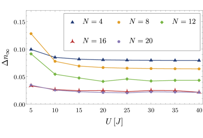
Figure 13: (Color online) Infinite-time averages of the jump $\Delta n_{\infty}$ calculated from (38). No pronounced dependence on $U$ is found except for weaker quenches $U<2W=8J$, see discussion in main text. The calculation shown is performed using the Lanczos algorithm with a maximum Krylov space dimension $f\leq 1000$.

The ensuing data for various system sizes is displayed in Fig. 13 in dependence on the quenched interaction strength $U$. Clearly, for larger values of $U$, no noticeable dependence on $U$ arises. The stronger dependence for smaller values of $U\approx 5J$ can be attributed to the slower decay of the jump, see Fig. 9. If the decay is slow, the revivals are larger. Hence, for smaller system sizes the jump seems to be larger. We emphasize that the infinite-time averages also comprise all the effects of revivals. Consequently, it is explainable that the infinite-time averages are finite in spite of the observation that they vanish rapidly, see Fig. 9.

If the above sketched view is correct, larger systems with later and weaker revivals should show smaller values of $\Delta n_{\infty}$. Thus, we aim at a finite-size extrapolation. In order not to do such an extrapolation for many different values of $U$ we use the fact that they hardly depend on $U$ as long as it is large, see Fig. 13. We average $\Delta n_{\infty}$ in the interaction interval $U\in[15J,40J]$ and plot the results as function of the inverse system size $1/N$ in Fig. 14.

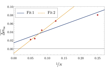
Figure 14: (Color online) Mean values $\overline{\Delta n_{\infty}}$ of the infinite-time jump $\Delta n_{\infty}$ averaged between $U=15J$ and $U=40J$ vs. the inverse lattice size. The linear fit 1 (2) includes (excludes) the data point for $N=4$.

For extrapolation we employ linear fits. There are not enough points and they scatter a bit so that the accuracy of the extrapolation is limited to about 2%. But fit 2, excluding the very small system size of $N=4$ sites, yields a value close to zero, though negative, but very small. The fit 1, including the case $N=4$, yields a small positive value. The difference of both extrapolated values yields an estimate for the accuracy which is about $0.02$. Clearly, the extrapolations are fully consistent with $\Delta n_{\infty}=0$ for the thermodynamic limit, i.e., for $N=\infty$. We stress that this finding is the same that we concluded already previously from the analysis of Fig. 9.

V Summary

In the present article, progress has been achieved in two main domains.

The first domain is conceptual. We presented a general approach to compute time-dependent expectation values based on time-dependent operators in the Heisenberg picture with truncated bases. The key idea is to choose an appropriate scalar product for operators such that the Liouville operator, i.e., commutation with the Hamiltonian, is self-adjoint. We presented such a suitable choice based on the Frobenius scalar product for a fermionic model. An application to spin models has been published elsewhere Röhrig et al. (2018). As noted before Kalthoff et al. (2017), however, this approach only works as such for finite local Hilbert spaces, i.e., for lattice models of fermions and spins.

On the conceptual side, we, moreover, showed that the self-adjoint Liouville operator implies a unitarity of the time evolution on the operator level. Generically, this implies oscillatory behavior as it has to be in quantum mechanics. We discussed comprehensively that the usual unitarity on the level of states is clearly distinct. Indeed, the latter implies operator unitarity, but the operator unitarity does not imply state unitarity.

Based on the operator unitary time evolution we used the concept of stationary phases to derive equations which directly express the expectation values of the (quasi-)stationary state to which the system converges for infinite time. The prefix “quasi” expresses that one cannot be sure that this state does not still show oscillations. In finite systems, we would indeed expect that oscillations persist. But they typically decrease upon increasing system size.

The second domain is the concrete application of the abstract concepts developed in the first domain to a fermionic model. For simplicity, we choose the one-dimensional Hubbard model and studied an interaction quench from the non-interacting Fermi sea to some finite interaction $U$. The integrability of the model is not used at any stage.

We conceived the $3^{+}$-basis. This basis describes all possible physical processes which can occur on up to three lattice sites. It is designed to capture the limit of strong interactions and small hopping; it is exact up to order $(J/U)^{2}$. The performance of this orthonormal operator basis (ONOB) was tested by computing the local particle number. Rigorously, it should be constant and equal to the filling factor. In the truncated approach, however, this need not be the case. But we showed that the $3^{+}$-basis reproduces the filling factor to good accuracy. For large values of $U$ the agreement is even very good.

Then, we computed the time evolution of the momentum distribution. It is dominated by out-of-phase oscillations of the initially occupied and unoccupied momenta. These oscillations correspond to Rabi oscillations, well-known from two-level systems. They are reminiscent of the collapse-and-revival scenario in bosonic systems Greiner et al. (2002) and they were observed before in the one-dimensional Hamerla and Uhrig (2013a), the two-dimensional Hubbard model Hamerla and Uhrig (2014), and the infinite-dimensional Hubbard model Eckstein, Kollar, and Werner (2009).

Finally, we focussed on the Fermi jump, i.e., the discontinuity of the momentum distribution at the Fermi wave vectors. Here we showed that the oscillations quickly die out. Finite-size effects are completely controllable. A systematic frequency analysis shows that two important frequencies/energies dominate: the band width $W$ and the interaction $U$. Interestingly, we do not find a singular dynamic phase transition as function of the quenched interaction, but a smooth crossover. Spectral features gain and lose weight, but they do not pop up or vanish suddenly. This is in contrast to previous interpretations. This progress has become possible due to the significantly longer accessible times thanks to the conceptual progress in the first domain.

VI Outlook

Optimizing the code will enable one to tackle significantly larger systems. Then, a quantitative analysis of the decay times at the Fermi wave vector and far away from it will be possible and is called for. This can be done in one dimension, but since no special feature of the one-dimensionality has been exploited, the same objectives can be pursued for two-dimensional systems. Of course, the accessible linear sizes will be more limited.

Another important route to follow is to enlarge the operator basis, for instance from three to five sites. Then, it should be possible to study the relaxation of weak quenches, i.e., the regime $U/J\ll 1$. This regime is in principle also accessible to perturbative, diagrammatic approaches which opens the way to direct comparisons.

Finally, we stress that different initial conditions can also be implemented by adjusting the matrix $\mathbf{A}$. From the conceptual point of view, this is straightforward. For instance, initial states which are relatively simple product states can be accounted for easily, even if they break a symmetry, e.g., spin or translational symmetry. More work has to be done in order to determine the initial correlations in strongly correlated systems. These require an equilibrium calculation in the first place in order to know the initial conditions.

In summary, there is a plethora of questions to address so that we are confident that the field of non-equilibrium quantum physics will continue to thrive.

Appendix A Basis operators

For completeness, we provide the full $3^{+}$-basis which is used mainly in this article. This basis is closed, i.e., invariant under iterated application of $\mathcal{L}_{\text{int}}\!\left(\cdot\right)$. Consequently, it is well-suited to study the regime $\nicefrac{{J}}{{U}}\ll 1$, i.e., comparatively strong quenches.

The following orthonormal basis operators have to be added to the two given in Eq. 40, eventually leading to nine different operator families in total in the complete $3^{+}$-basis.

Restrictions regarding the site indices apply. The following operators exist for three distinct indices $i\neq j\neq k$, $i\neq k$. Note that the operators $w_{3}^{\dagger}(i,j,k)$ also exist for the case where only $i$ is distinct from the other two indices. The same applies to $w_{4}^{\dagger}(i,j,k)$ for the index $j$ and $w_{5}^{\dagger}(i,j,k)$ for the index $k$.

$$w_{3}^{\dagger}(i,j,k) =\left(\!\sqrt{2}\right)^{5}f_{i\uparrow}^{\dagger}\left(\widehat{n}_{i\downarrow}^{\vphantom{\dagger}}-\frac{1}{2}\right)\left(f_{j\downarrow}^{\dagger}f_{k\downarrow}^{\vphantom{\dagger}}-\frac{1}{2}\delta_{jk}\right)$$ (48a)

$$w_{4}^{\dagger}(i,j,k) =\left(\!\sqrt{2}\right)^{5}f_{i\uparrow}^{\dagger}f_{j\downarrow}^{\dagger}\left(\widehat{n}_{j\uparrow}^{\vphantom{\dagger}}-\frac{1}{2}\right)f_{k\downarrow}^{\vphantom{\dagger}}$$ (48b)

$$w_{5}^{\dagger}(i,j,k) =\left(\!\sqrt{2}\right)^{5}f_{i\uparrow}^{\dagger}f_{j\downarrow}^{\dagger}f_{k\downarrow}^{\vphantom{\dagger}}\left(\widehat{n}_{k\uparrow}^{\vphantom{\dagger}}-\frac{1}{2}\right)$$ (48c)

$$w_{6}^{\dagger}(i,j,k) =\left(\!\sqrt{2}\right)^{7}f_{i\uparrow}^{\dagger}\left(\widehat{n}_{i\downarrow}^{\vphantom{\dagger}}-\frac{1}{2}\right)f_{j\downarrow}^{\dagger}\left(\widehat{n}_{j\uparrow}^{\vphantom{\dagger}}-\frac{1}{2}\right)f_{k\downarrow}^{\vphantom{\dagger}}$$ (48d)

$$w_{7}^{\dagger}(i,j,k) =\left(\!\sqrt{2}\right)^{7}f_{i\uparrow}^{\dagger}\left(\widehat{n}_{i\downarrow}^{\vphantom{\dagger}}-\frac{1}{2}\right)f_{j\downarrow}^{\dagger}f_{k\downarrow}^{\vphantom{\dagger}}\left(\widehat{n}_{k\uparrow}^{\vphantom{\dagger}}-\frac{1}{2}\right)$$ (48e)

$$w_{8}^{\dagger}(i,j,k) =\left(\!\sqrt{2}\right)^{7}f_{i\uparrow}^{\dagger}f_{j\downarrow}^{\dagger}\left(\widehat{n}_{j\uparrow}^{\vphantom{\dagger}}-\frac{1}{2}\right)f_{k\downarrow}^{\vphantom{\dagger}}\left(\widehat{n}_{k\uparrow}^{\vphantom{\dagger}}-\frac{1}{2}\right)$$ (48f)

$$w_{9}^{\dagger}(i,j,k) =\left(\!\sqrt{2}\right)^{9}f_{i\uparrow}^{\dagger}\left(\widehat{n}_{i\downarrow}^{\vphantom{\dagger}}-\frac{1}{2}\right)f_{j\downarrow}^{\dagger}\left(\widehat{n}_{j\uparrow}^{\vphantom{\dagger}}-\frac{1}{2}\right)f_{k\downarrow}^{\vphantom{\dagger}}\left(\widehat{n}_{k\uparrow}^{\vphantom{\dagger}}-\frac{1}{2}\right).$$ (48g)

This completes the orthonormal $3^{+}$-basis of operators.

References

- Anderson and Kasevich (1998) B. P. Anderson and M. A. Kasevich, Science 282, 1686 (1998).
- Bloch (2005) I. Bloch, Nat. Phys. 1, 23 (2005).
- Trotzky et al. (2012) S. Trotzky, Y. A. Chen, A. Flesch, I. P. McCulloch, U. Schollwöck, J. Eisert, and I. Bloch, Nat. Phys. 8, 325 (2012).
- Greiner et al. (2002) M. Greiner, O. Mandel, T. Esslinger, T. W. Hänsch, and I. Bloch, Nature 415, 39 (2002).
- Goldman, Budich, and Zoller (2016) N. Goldman, J. C. Budich, and P. Zoller, Nat. Phys. 12, 639 (2016).
- Axt and Kuhn (2004) V. M. Axt and T. Kuhn, Reports Prog. Phys. 67, 433 (2004).
- Morawetz (2004) K. Morawetz, Nonequilibrium Physics at Short Time Scales, edited by K. Morawetz (Springer Berlin Heidelberg, Berlin, Heidelberg, 2004).
- Perfetti et al. (2006) L. Perfetti, P. A. Loukakos, M. Lisowski, U. Bovensiepen, H. Berger, S. Biermann, P. S. Cornaglia, A. Georges, and M. Wolf, Phys. Rev. Lett. 97, 067402 (2006).
- Stöferle et al. (2004) T. Stöferle, H. Moritz, C. Schori, M. Köhl, and T. Esslinger, Phys. Rev. Lett. 92, 130403 (2004).
- Sherson et al. (2010) J. F. Sherson, C. Weitenberg, M. Endres, M. Cheneau, I. Bloch, and S. Kuhr, Nature 467, 68 (2010).
- Sanders, Mintert, and Heller (2010) S. N. Sanders, F. Mintert, and E. J. Heller, Phys. Rev. Lett. 105, 035301 (2010).
- Mayer, Rodriguez, and Buchleitner (2014) K. Mayer, A. Rodriguez, and A. Buchleitner, Phys. Rev. A 90, 023629 (2014).
- Mekhov, Maschler, and Ritsch (2007) I. B. Mekhov, C. Maschler, and H. Ritsch, Nat. Phys. 3, 319 (2007).
- ten Brinke and Schützhold (2015) N. ten Brinke and R. Schützhold, Phys. Rev. A 92, 013617 (2015).
- Strohmaier et al. (2010) N. Strohmaier, D. Greif, R. Jördens, L. Tarruell, H. Moritz, T. Esslinger, R. Sensarma, D. Pekker, E. Altman, and E. Demler, Phys. Rev. Lett. 104, 080401 (2010).
- Lenarčič and Prelovšek (2013) Z. Lenarčič and P. Prelovšek, Phys. Rev. Lett. 111, 016401 (2013).
- Mattuck (1976) R. D. Mattuck, A guide to Feynman diagrams in the many-body problem (Dover Publications, New York, 1976).
- Läuchli and Kollath (2008) A. M. Läuchli and C. Kollath, J. Stat. Mech. Theory Exp. 2008, P05018 (2008).
- Chen et al. (2011) D. Chen, M. White, C. Borries, and B. DeMarco, Phys. Rev. Lett. 106, 235304 (2011).
- Langen et al. (2013) T. Langen, R. Geiger, M. Kuhnert, B. Rauer, and J. Schmiedmayer, Nat. Phys. 9, 640 (2013).
- Cazalilla (2006) M. A. Cazalilla, Phys. Rev. Lett. 97, 156403 (2006).
- Barthel and Schollwöck (2008) T. Barthel and U. Schollwöck, Phys. Rev. Lett. 100, 100601 (2008).
- Calabrese, Essler, and Fagotti (2011) P. Calabrese, F. H. L. Essler, and M. Fagotti, Phys. Rev. Lett. 106, 227203 (2011).
- Calabrese, Essler, and Fagotti (2012a) P. Calabrese, F. H. L. Essler, and M. Fagotti, J. Stat. Mech. Theory Exp. 2012, P07022 (2012a).
- Calabrese, Essler, and Fagotti (2012b) P. Calabrese, F. H. L. Essler, and M. Fagotti, J. Stat. Mech. Theory Exp. , P07022 (2012b).
- Caux and Essler (2013) J.-S. Caux and F. H. L. Essler, Phys. Rev. Lett. 110, 257203 (2013).
- Rigol (2009) M. Rigol, Phys. Rev. A 80, 053607 (2009).
- Eckstein, Kollar, and Werner (2009) M. Eckstein, M. Kollar, and P. Werner, Phys. Rev. Lett. 103, 056403 (2009).
- Aoki et al. (2014) H. Aoki, N. Tsuji, M. Eckstein, M. Kollar, T. Oka, and P. Werner, Rev. Mod. Phys. 86, 779 (2014).
- Navez and Schützhold (2010) P. Navez and R. Schützhold, Phys. Rev. A 82, 063603 (2010).
- Krutitsky et al. (2014) K. V. Krutitsky, P. Navez, F. Queisser, and R. Schützhold, EPJ Quantum Technol. 1, 12 (2014).
- White and Feiguin (2004) S. R. White and A. E. Feiguin, Phys. Rev. Lett. 93, 076401 (2004).
- Daley et al. (2004) A. J. Daley, C. Kollath, U. Schollwöck, and G. Vidal, J. Stat. Mech. Theory Exp. 2004, P04005 (2004).
- Batrouni et al. (2005) G. G. Batrouni, F. F. Assaad, R. T. Scalettar, and P. J. H. Denteneer, Phys. Rev. A 72, 031601(R) (2005).
- Goth and Assaad (2012) F. Goth and F. F. Assaad, Phys. Rev. B 85, 085129 (2012).
- Schiró and Fabrizio (2010) M. Schiró and M. Fabrizio, Phys. Rev. Lett. 105, 076401 (2010).
- Schiró and Fabrizio (2011) M. Schiró and M. Fabrizio, Phys. Rev. B 83, 165105 (2011).
- Ido, Ohgoe, and Imada (2015) K. Ido, T. Ohgoe, and M. Imada, Phys. Rev. B 92, 245106 (2015).
- Moeckel and Kehrein (2008) M. Moeckel and S. Kehrein, Phys. Rev. Lett. 100, 175702 (2008).
- Moeckel and Kehrein (2009) M. Moeckel and S. Kehrein, Ann. Phys. (N. Y). 324, 2146 (2009).
- Sabio and Kehrein (2010) J. Sabio and S. Kehrein, New J. Phys. 12, 055008 (2010).
- Uhrig (2009) G. S. Uhrig, Phys. Rev. A 80, 061602(R) (2009).
- Hamerla and Uhrig (2013a) S. A. Hamerla and G. S. Uhrig, Phys. Rev. B 87, 064304 (2013a).
- Hamerla and Uhrig (2013b) S. A. Hamerla and G. S. Uhrig, New J. Phys. 15, 073012 (2013b).
- Hamerla and Uhrig (2014) S. A. Hamerla and G. S. Uhrig, Phys. Rev. B 89, 104301 (2014).
- Kalthoff et al. (2017) M. Kalthoff, F. Keim, H. Krull, and G. S. Uhrig, Eur. Phys. J. B 90, 97 (2017).
- Röhrig et al. (2018) R. Röhrig, P. Schering, L. B. Gravert, and G. S. Uhrig, Phys. Rev. B (in press) (2018), arXiv:1711.08919 .
- Lieb and Wu (1968) E. H. Lieb and F. Y. Wu, Phys. Rev. Lett. 20, 1445 (1968).
- Faddeev (2005) L. D. Faddeev, The Bethe ansatz (Cambridge University Press, Cambridge, 2005).
- Hubbard (1963) J. Hubbard, Proc. R. Soc. A Math. Phys. Eng. Sci. 276, 238 (1963).
- Kanamori (1963) J. Kanamori, Prog. Theor. Phys. 30, 275 (1963).
- Gutzwiller (1963) M. C. Gutzwiller, Phys. Rev. Lett. 10, 159 (1963).
- Manmana et al. (2007) S. R. Manmana, S. Wessel, R. M. Noack, and A. Muramatsu, Phys. Rev. Lett. 98, 210405 (2007).
- Manmana et al. (2009) S. R. Manmana, S. Wessel, R. M. Noack, and A. Muramatsu, Phys. Rev. B 79, 155104 (2009).
- Barmettler et al. (2009) P. Barmettler, M. Punk, V. Gritsev, E. Demler, and E. Altman, Phys. Rev. Lett. 102, 130603 (2009).
- Lieb and Robinson (1972) E. H. Lieb and D. W. Robinson, Commun. Math. Phys. 28, 251 (1972).
- Jurcevic et al. (2014) P. Jurcevic, B. P. Lanyon, P. Hauke, C. Hempel, P. Zoller, R. Blatt, and C. F. Roos, Nature 511, 202 (2014).
- Hauke and Tagliacozzo (2013) P. Hauke and L. Tagliacozzo, Phys. Rev. Lett. 111, 207202 (2013).
- Eisert et al. (2013) J. Eisert, M. van den Worm, S. R. Manmana, and M. Kastner, Phys. Rev. Lett. 111, 260401 (2013).
- Jünemann et al. (2013) J. Jünemann, A. Cadarso, D. Pérez-García, A. Bermudez, and J. J. García-Ripoll, Phys. Rev. Lett. 111, 230404 (2013).
- Wick (1950) G. C. Wick, Phys. Rev. 80, 268 (1950).
- Fioretto and Mussardo (2010) D. Fioretto and G. Mussardo, New J. Phys. 12, 055015 (2010).
- Lanczos (1938) C. Lanczos, Studies in Applied Mathematics 17, 123 (1938).
- Arnoldi (1951) W. E. Arnoldi, Quarterly Appl. Math. 9, 17 (1951).
- Damascelli, Shen, and Hussain (2003) A. Damascelli, Z.-X. Shen, and Z. Hussain, Rev. Mod. Phys. 75, 473 (2003).
- Bloch, Dalibard, and Zwerger (2008) I. Bloch, J. Dalibard, and W. Zwerger, Rev. Mod. Phys. 80, 885 (2008).
- Hamerla (2013) S. A. Hamerla, Dynamics of Fermionic Hubbard Models after Interaction Quenches in One and Two Dimensions, Phd thesis, Technische Universität Dortmund (2013).