Partial-Wave Analysis of $\gamma p\rightarrow K^{+}\Lambda$ using a multichannel framework

Abstract

Results from a partial-wave analysis of the reaction $\gamma p\rightarrow K^{+}\Lambda$  are presented. The reaction is dominated by the $S_{11}(1650)$ and $P_{13}(1720)$ resonances at low energies and by $P_{13}(1900)$ at higher energies. There are small contributions from all amplitudes up to and including $G_{17}$, with $F_{17}$ necessary for obtaining a good fit of several of the spin observables. We find evidence for $P_{11}$(1880), $D_{13}$(2120), and $D_{15}$(2080) resonances, as well as a possible $F_{17}$ resonance near 2300 MeV, which is expected from quark-model predictions. Some predictions for $\gamma n\to K^{0}\Lambda$ are also included.

I Introduction

Quark models predict a larger number of resonances than have been experimentally verified. This is called the problem of the “missing resonances.” One possible explanation is that these resonances decouple from the $\pi N$ channel. Photoproduction reactions involving final states other than $\pi N$ provide an opportunity to search for these resonances.

One of the best measured of these reactions is $\gamma p\to K^{+}\Lambda$. Of the 16 single- and double-polarization observables, eight have been measured and published while the others are in some stage of analysis. With measurements of so many observables, it might be expected that only a single unique solution is permitted by the data; however, there are still major discrepancies between the amplitudes determined by different groups. One encouragement is that the predicted resonance spectrum is in good agreement. This paper is laid out as follows: Sec. II describes the formalism and methodology for the partial-wave analysis, Sec. III describes the procedure used, Sec. IV describes results from the analysis, and Sec. V presents a summary and conclusions. Finally, Appendix A compares our final energy-dependent solution with the data included in our analysis.

II Formalism and Methodology

Four helicity amplitudes describe the photoproduction of a pseudoscalar ($J^{P}=0^{-}$) meson and a $J^{P}=\frac{1}{2}^{+}$ baryon off of a nucleon target Walker . Each of the four helicity amplitudes can be expanded in terms of electric and magnetic multipoles $E_{l\pm}$ and $M_{l\pm}$, respectively, where $l=0,1,2,...$ is the orbital angular momentum of the final-state hadrons and $j=l\pm\frac{1}{2}$ is the total angular momentum. Each multipole is a complex function of energy, which makes the helicity amplitudes complex functions of both energy and scattering angle:

$$H_{N}=\sqrt{\frac{1}{2}}\cos\left(\frac{\theta}{2}\right)\sum_{l=0}^{\infty}\left[\left(l+2\right)E_{l+}+lM_{l+}\right.\\ +lE_{\left(l+1\right)-}-\left(l+2\right)M_{\left(l+1\right)-}\left.\right]\left(P_{l}^{{}^{\prime}}-P_{l+1}^{{}^{\prime}}\right),$$ (1a)

$$H_{SP}=\sqrt{\frac{1}{2}}\cos\left(\frac{\theta}{2}\right)\sin(\theta)\sum_{l=1}^{\infty}\left[E_{l+}-M_{l+}\right]\\ -E_{\left(l+1\right)-}-M_{\left(l+1\right)-}\left.\right]\left(P_{l}^{{}^{\prime\prime}}-P_{l+1}^{{}^{\prime\prime}}\right),$$ (1b)

$$H_{SA}=\sqrt{\frac{1}{2}}\sin\left(\frac{\theta}{2}\right)\sum_{l=0}^{\infty}\left[\left(l+2\right)E_{l+}\right.+lM_{l+}\\ -lE_{\left(l+1\right)-}+\left(l+2\right)M_{\left(l+1\right)-}\left.\right]\left(P_{l}^{{}^{\prime}}+P_{l+1}^{{}^{\prime}}\right),$$ (1c)

$$H_{D}=\sqrt{\frac{1}{2}}\sin\left(\frac{\theta}{2}\right)\sin(\theta)\sum_{l=1}^{\infty}\left[E_{l+}-M_{l+}\right.\\ +E_{\left(l+1\right)-}+M_{\left(l+1\right)-}\left.\right]\left(P_{l}^{{}^{\prime\prime}}+P_{l+1}^{{}^{\prime\prime}}\right).$$ (1d)

The naming convention for the four helicity amplitudes in Eq. (II) follows that of the SAID group SAID1990 . All 16 single- and double-polarization observables can be written in terms of these four helicity amplitudes; however, in the literature, different sign conventions are used in their definitions. The signs used for the observables in this work are listed in Table 1 and also follow the conventions of the SAID group.

$\sigma(\theta)=\frac{q}{2k}\left[|H_{N}|^{2}+|H_{D}|^{2}+|H_{SA}|^{2}+|H_{SP}|^{2}\right]$
$\Sigma\>\sigma(\theta)=\frac{q}{k}\text{Re}\left[H_{SP}H_{SA}^{*}-H_{N}H_{D}^{*}\right]$	$B$
$T\>\sigma\left(\theta\right)=\frac{q}{k}\text{Im}\left[H_{SP}H_{N}^{*}+H_{D}H_{SA}^{*}\right]$	$T$
$P\>\sigma\left(\theta\right)=-\frac{q}{k}\text{Im}\left[H_{SP}H_{D}^{*}+H_{N}H_{SA}^{*}\right]$	$R$
$G\>\sigma\left(\theta\right)=-\frac{q}{k}\text{Im}\left[H_{SP}H_{SA}^{*}+H_{N}H_{D}^{*}\right]$	$B$, $T$
$H\>\sigma\left(\theta\right)=-\frac{q}{k}\text{Im}\left[H_{SP}H_{D}^{*}+H_{SA}H_{N}^{*}\right]$	$B$, $T$
$F\>\sigma\left(\theta\right)=\frac{q}{k}\text{Re}\left[H_{SA}H_{D}^{*}+H_{SP}H_{N}^{*}\right]$	$B$, $T$
$E\>\sigma\left(\theta\right)=\frac{q}{2k}\left[|H_{N}|^{2}+|H_{SA}|^{2}-|H_{D}|^{2}-|H_{SP}|^{2}\right]$	$B$, $T$
$O_{x}\>\sigma\left(\theta\right)=-\frac{q}{k}\text{Im}\left[H_{SA}H_{D}^{*}+H_{SP}H_{N}^{*}\right]$	$B$, $R$
$O_{z}\>\sigma\left(\theta\right)=-\frac{q}{k}\text{Im}\left[H_{SA}H_{SP}^{*}+H_{N}H_{D}^{*}\right]$	$B$, $R$
$C_{x}\>\sigma\left(\theta\right)=-\frac{q}{k}\text{Re}\left[H_{SA}H_{N}^{*}+H_{SP}H_{D}^{*}\right]$	$B$, $R$
$C_{z}\>\sigma\left(\theta\right)=\frac{q}{2k}\left[|H_{SA}|^{2}+|H_{D}|^{2}-|H_{N}|^{2}-|H_{SP}|^{2}\right]$	$B$, $R$
$T_{x}\>\sigma\left(\theta\right)=\frac{q}{k}\text{Re}\left[H_{SP}H_{SA}^{*}+H_{N}H_{D}^{*}\right]$	$T$, $R$
$T_{z}\>\sigma\left(\theta\right)=\frac{q}{k}\text{Re}\left[H_{SP}H_{N}^{*}-H_{SA}H_{D}^{*}\right]$	$T$, $R$
$L_{x}\>\sigma\left(\theta\right)=\frac{q}{k}\text{Re}\left[H_{SA}H_{N}^{*}-H_{SP}H_{D}^{*}\right]$	$T$, $R$
$L_{z}\>\sigma\left(\theta\right)=\frac{q}{2k}\left[|H_{SP}|^{2}+|H_{SA}|^{2}-|H_{N}|^{2}-|H_{D}|^{2}\right]$	$T$, $R$

Table 1: List of single-polarization and double-polarization observables analyzed in this work. See Refs. BDS1 ; Sandorfi for a detailed description of the necessary experimental setup and equations for all 16 observables. In the second column, $B$, $T$, and $R$ refer to a measurement of the beam, target, and recoil nucleon polarization, respectively. Note that $\sigma\left(\theta\right)=d\sigma/d\Omega$ is the differential cross section.

The literature also mentions measurements of ${d\sigma}/{d\Omega}_{\frac{1}{2}}$ and ${d\sigma}/{d\Omega}_{\frac{3}{2}}$, which are the helicity-dependent cross sections. These observables are linear combinations of the differential cross section and $E$ observables.

III Procedure

Before the analysis could be initiated, some data sets needed modification from their published form. $C_{x}$ and $C_{z}$ data from Bradford et al. Bradford06 were rotated by an angle of $\pi+\theta_{cm}$ from their published form. Here, $\theta_{cm}$ is the polar angle of the outgoing $K^{+}$ meson in the center-of-momentum frame. (The inverse rotation is given in Eq. 2 in Lleres et al. Lleres09 ). When comparing this work with other works, this rotation may also need to be combined with a sign change due to different observable conventions. A “Rosetta Stone” that describes different conventions is discussed in Sandorfi et al. Sandorfi2 . This work follows the conventions of the SAID/GWU group for all 16 polarization observables.) $O_{x}$ and $O_{z}$ data obtained from Paterson et al. Paterson16 required the same rotation. After rotation, the Paterson data agree with a previous measurement by Lleres et al. Lleres09 . The $L_{z}$ data from Casey CaseyPhD needed to be multiplied by $-1$ due to the $z^{\prime}$ axis being flipped and a difference in sign conventions between groups. SAPHIR $d\sigma/d\Omega$ measurements from Tran et al.  Tran98 and Glander et al.  Glander04 were removed, as well as a dataset from Hicks et al.  Hicks07 . Finally, data below 1639 MeV from Jude et al.  Jude14 were also removed.

To begin the analysis, all data were binned into specified small c.m. energy ranges. Observables within a single bin were then approximated as functions of just the scattering angle. An appropriate bin width was determined by initially binning the observables into wide bins of 100 MeV and noticing that there was little variation in the double-polarization data over the energy range of the analysis. This meant that 20-MeV wide bins were sufficient to describe the energy variation in the observables near threshold where the $S_{11}$ and $P_{13}$ amplitudes dominate due to the $S_{11}$(1650) and $P_{13}$(1720) resonances. At c.m. energies from 1850 to 2200 MeV where resonances are expected to have wider widths, 40 MeV bins were used.

Once the data were binned, an initial round of single-energy fits was performed in which the $S_{11}$ amplitude was kept real to determine its magnitude. Then a multichannel energy-dependent fit, similiar to those of Shrestha and Manley ShresthaED , was performed to determine the $S_{11}$ phase through unitarity constraints. With the $S_{11}$ amplitude fully determined, initial values for the higher-order amplitudes were then determined. An iterative procedure in which we first carried out single-energy fits, followed by a set of multichannel energy-dependent fits of individual partial waves, was used to obtain convergence of the solution to a global minimum.

Because not all measured observables are available in all energy bins, $\chi^{2}$ penalty terms were added to the standard $\chi^{2}$ term to constrain the single-energy solutions. The explicit form for a penalty term was

$$\chi^{2}_{\text{penalty}}=f[(PW^{R}_{\text{ED}}-PW^{R}_{\text{fit}})^{2}+f^{I}(PW^{I}_{\text{ED}}-PW^{I}_{\text{fit}})^{2}],$$ (2)

where $PW^{R}_{\text{ED}}$ and $PW^{I}_{\text{ED}}$ are the real and imaginary parts of the partial-wave amplitude found in the preceding energy-dependent fit and $PW^{R}_{\text{fit}}$ and $PW^{I}_{\text{fit}}$ are the corrsponding real and imaginary parts of the amplitude determined during each step of the single-energy fit. The factor $f$ was a parameter chosen to control the strength of the penalty term. For the initial round of single-energy fits, we set $f=0$ for no penalty term at all. After the first round of energy-dependent fits, we used values from the energy-dependent fits to constrain selected partial waves in the next round of single-energy fits. This was initially done with a weak penalty constraint (e.g., $f=10$), but as iterations progressed and the energy-dependent solutions did a better job of describing the fitted observables, we gradually increased the strength of the penalty term (e.g., to $f=30$ or $f=50$). This biased results to single-energy solutions that were somewhat similar to the current energy-dependent solution. To minimize bias from the penalty terms, multiple starting solutions were used to determine which produced the best fit. During the analysis, the $\chi^{2}$ penalty contribution typically remained below a few percent of the total $\chi^{2}$.

Once the constrained single-energy solutions converged to agree with the final energy-dependent solution, final error bars on the single-energy amplitudes were obtained by performing “zero-iteration” fits in which the phases of the amplitudes were held fixed and only their moduli were allowed to vary. During this step, the penalty terms were removed from the analysis.

IV Results

This section presents final results for the partial-wave analysis of $\gamma p\rightarrow K^{+}\Lambda$  and predictions for the reaction $\gamma n\rightarrow K^{0}\Lambda$ . It compares our results with those of the BnGa group and shows the quality of agreement with integrated cross-section data , which were not directly fitted. Table 2 shows the $\chi^{2}$ breakdown by observable and compares our results with the BnGa 2016 solution. The table also lists references for each observable included in the single-energy fits.

The resonances that were found to contribute significantly in our multichannel energy-dependent fits were the $S_{11}$(1650), $P_{11}$(1880), $P_{13}$(1720), $P_{13}$(1900), $D_{13}$(2120), and $D_{15}$(2080). This is similar to the resonance structure found by other groups. There was some indication in the data of a possible $F_{17}$ resonance around 2300 MeV that was also seen in pion photoproduction. This is in agreement with quark-model predictions Capstick98 that a higher-lying $F_{17}$ resonance should couple to $K\Lambda$.

Observable	KSU	BnGa (2016)	No. Data	References
$d\sigma/d\Omega$	8400	9500	4101	Donoho58 ; Brody60 ; Anderson62 ; Peck64 ; Anderson65 ; Mori66 ; Groom67 ; Bleckmann70 ; Decamp70 ; Fujii70 ; Goeing71 ; Feller72 ; Bockhorst94 ; Mcnabb04 ; Bradford06 ; Sumihama06 ; Mccracken10 ; Jude14
$T$	3000	2100	451	Althoff78 ; Lleres09 ; WolfordPhD ; Paterson16
$\Sigma$	2400	1200	418	Zegers03 ; Sumihama06 ; Lleres07 ; Paterson16
$P$	3200	3200	1565	Mcdaniel59 ; Thom63 ; Borgia64 ; Grilli65 ; Groom67 ; Fujii70 ; Haas78 ; Bockhorst94 ; Mcnabb04 ; Lleres07 ; Mccracken10 ; Paterson16
$F$	990	5300	(84)	WolfordPhD
$E$	2500	330	(72)	CaseyPhD
$C_{x}$	310	230	97	Bradford07
$C_{z}$	430	210	97	Bradford07
$O_{x}$	1000	460	363	Lleres09 ; Paterson16
$O_{z}$	1500	650	363	Lleres09 ; Paterson16
$T_{x}$	1000	4200	(77)	WolfordPhD
$T_{z}$	1300	2700	(53)	WolfordPhD
$L_{x}$	90	95	(87)	CaseyPhD
$L_{z}$	230	180	(72)	CaseyPhD
Fit Total	26000	30000

Table 2: Comparison of $\chi^{2}$ contributions to $\gamma p\to K^{+}\Lambda$ for different observables and analyses. Column one lists the observable, columns two and three list the $\chi^{2}$ contribution from each observable, column four lists the number of published (unpublished) data points for the observable, and column five lists references for the observable. See text for information on binning changes and discussion on the points included. The c.m. energy range and binning used to generate the $\chi^{2}$ values was $W=1610$ - 2200 MeV in 10-MeV wide bins.

The integrated cross section for $\gamma p\rightarrow K^{+}\Lambda$  is dominated by the $S_{11}$ amplitude at low energies and the $P_{13}$ amplitude at higher energies. The cross section is then saturated by small contributions from the other partial waves up to and including $G_{19}$, which was the highest partial wave included in our fits of $\gamma p\rightarrow K^{+}\Lambda$ data. There is excellent agreement between the results of the analysis and the data. Figures 1, 2, and 3 show the integrated cross section as well as predictions of the helicity-1/2 and -3/2 integrated cross sections. The helicity-3/2 cross section is predicted to be strongly dominated by the $P_{13}$ multipoles.

Plots comparing the partial-wave amplitudes for this reaction are shown in Fig. 4, with comparisons only available between this work and BnGa 2016 Sarantsev .

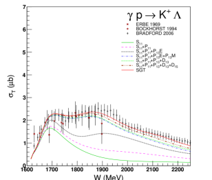
Figure 1: Integrated cross section for $\gamma p\rightarrow K^{+}\Lambda$ . The curves show the contribution to the cross section by successively adding each partial wave. Points are from ERBE 1969 Erbe69 , BOCKHORST 1994 Bockhorst94 , and BRADFORD 2006 Bradford06 .

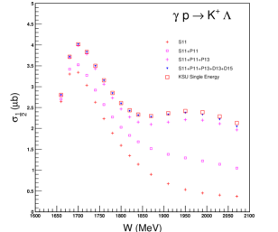
Figure 2: Prediction of helicity-$1/2$ integrated cross section for $\gamma p\rightarrow K^{+}\Lambda$ . The plot shows the predicted contribution to the cross section by successively adding each partial wave.

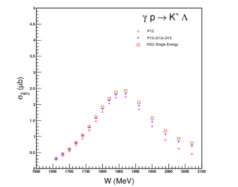
Figure 3: Prediction of helicity-$3/2$ integrated cross section for $\gamma p\rightarrow K^{+}\Lambda$ . The plot shows the predicted contribution to the cross section by successively adding each partial wave.

$S_{11}$ is the only amplitude from this work that agrees with results from the BnGa group. This was unexpected because of the sizable number of spin observables that have been measured for $\gamma p\to K^{+}\Lambda$. However, not all discrepancies are large. For instance, differences in the $P_{11}M$ amplitude seem to be correlated with a different mass and width for its resonance parameters as the behavior in the two amplitudes is similar.

In the $P_{13}E$ amplitude, differences are more significant. Resonance behavior is expected around 1720 MeV based on the photo and $K\Lambda$ couplings. For a resonant amplitude, the real part should approach zero near the resonance and the imaginary part should peak, a behavior in the amplitude that is found in this work. An odd behavior is found in the BnGa results for the amplitude $P_{13}M$. At low energies the amplitude shows a behavior like a Born term (which only contains a real part), but is found in the imaginary part instead. Their real part, also does not show a turn towards zero near the resonance. This suggests that perhaps there may be a global phase problem with the BnGa solution at low energies.

Figure 5 shows predictions for the observables $G$ and $H$ for this work and BnGa 2016 at selected energies. Despite the large number of observables that have been measured, predictions of $G$ and $H$ still show significant disagreement over the full energy range.

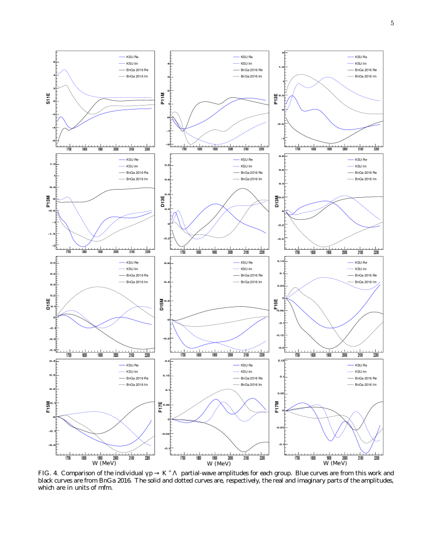
Figure 4: Comparison of the individual $\gamma p\rightarrow K^{+}\Lambda$  partial-wave amplitudes for each group. Blue curves are from this work and black curves are from BnGa 2016. The solid and dotted curves are, respectively, the real and imaginary parts of the amplitudes, which are in units of mfm.

Figure 5: The top four figures show predictions of the observable $G$ and the bottom four figures show predictions of the observable $H$ for $\gamma p\rightarrow K^{+}\Lambda$  at c.m. energies 1700, 1800, 1950, and 2150 MeV.

After completion of our analysis, we learned that $\gamma p\rightarrow K^{+}\Lambda$ has also been studied recently within the Jülich-Bonn (JüBo) coupled-channel framework Roenchen2018 . The level of agreement of the new JüBo solution with $d\sigma/d\Omega$, $\Sigma$, $P$, $O_{x}$, $O_{z}$, $C_{x^{\prime}}$, and $C_{z^{\prime}}$ data is quite good overall. Our solution tends to give a more isotropic differential cross section near threshold, although a detailed comparison of our solutions has not been evaluated. It is clear, however, that the multipoles in JüBo solution do not agree with those of either the BnGa group or with our solution. As noted previously, our $S_{11}$ amplitude qualitatively agrees with the BnGa results, whereas the $S_{11}$ (or $E_{0+}$) amplitude in the new JüBo solution agrees with neither our solution nor with the corresponding BnGa amplitude. Additional double-polarization data are probably needed to resolve these differences.

Because this analysis was carried out in conjunction with other photoproduction and hadronic reactions that included $\gamma n$ and $K\Lambda$ states, we are able to make predictions for $\gamma n\rightarrow K^{0}n$. The highest partial wave included in our predictions for $\gamma n\rightarrow K^{0}\Lambda$ was $F_{15}$ and our predictions are expected to be reasonable up to c.m. energies near 1900 MeV. Our predictions are compared to differential cross-section data by CLAS Compton2017 and Akondi AKONDIDiss in Fig. 6. Our prediction for the integrated cross section is shown in Fig. 7. The agreement is reasonably good with the $d\sigma/d\Omega$ CLAS data and Akondi results over most of the angular range below about 1800 MeV while there are a few places above that energy where the prediction has a bump at forward angles not seen in the data. The quality of agreement of our prediction with the CLAS Compton2017 and Akondi AKONDIDiss measurements suggests that the couplings to $\gamma n$ and $K\Lambda$ are highly constrained by the other reactions. It also lends credence to the fits presented in this work.

Figure 6: Predictions of $d\sigma/d\Omega$ for $\gamma n\rightarrow K^{0}\Lambda$ at $W$ = 1630 to 1855 MeV. Data points are from COMPTON 2017 Compton2017 and AKONDI 2018 AKONDIDiss .

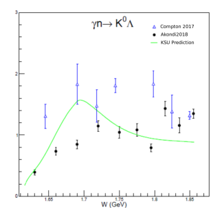
Figure 7: Predicted integrated cross section for $\gamma n\rightarrow K^{0}\Lambda$. The green curve shows our prediction and the data points are from COMPTON 2017 Compton2017 and AKONDI 2018 AKONDIDiss .

V Summary and Conclusions

This work presents results from a partial-wave analysis of $\gamma p\to K^{+}\Lambda$ and predictions for $\gamma n\to K^{0}\Lambda$. Results from previous works that $S_{11}$ and $P_{13}$ were the dominant amplitudes contributing to the integrated cross section were confirmed; however, the amplitudes from this work show more resonance-like behavior with less background than found by previous works. A potential second $F_{17}$ resonance near 2300 MeV was seen in this reaction as well as in $\pi N\rightarrow\pi N$ elastic scattering and $\gamma N\to\pi N$ photoproduction. More data above 2300 MeV are necessary to confirm its existence and its properties.

This work suggests that data for more than eight independent observables may be needed to reach a single unique solution for photoproduction reactions due to the large uncertainties in the double-polarization measurements and inconsistencies in the data.

The $\gamma p\to K^{+}\Lambda$ amplitudes from this work have been included in an updated multichannel energy-dependent partial-wave analysis paper3 that also incorporates our single-energy amplitudes for $\gamma p\rightarrow\eta p$ and $\gamma n\rightarrow\eta n$ paper1 . In Ref. paper3 , we present and discuss the resonance parameters obtained from a fit of single-energy amplitudes for these reactions combined with corresponding amplitudes for $\gamma N\rightarrow\pi N$, $\pi N\rightarrow\pi N$, $\pi N\rightarrow\pi\pi N$, $\pi N\rightarrow K\Lambda$, and $\pi N\rightarrow\eta N$. Reference paper3 also includes Argand diagrams that compare the results of our single-energy fits with our final energy-dependent partial-wave amplitudes.

Appendix A Final Fits to Experimental Data

Figures 8 - 27 compares our energy-dependent solution to the data included in our analysis. The partial-wave amplitudes used to generate the curves are available in the form of data files Datafile . Also shown in each figure are the fits from BnGa 2016 Sarantsev .

The sources for the data points found in the figures for this reaction are DONOHO 1958 Donoho58 , MCDANIEL 1959 Mcdaniel59 , BRODY 1960 Brody60 , ANDERSON 1962 Anderson62 , THOM 1963 Thom63 , BORGIA 1964 Borgia64 , PECK 1964 Peck64 , ANDERSON 1965 Anderson65 , GRILLI 1965 Grilli65 , MORI 1966 Mori66 , GROOM 1967 Groom67 , BLECKMANN 1970 Bleckmann70 , DECAMP 1970 Decamp70 , FUJII 1970 Fujii70 , GOING 1971 Goeing71 , FELLER 1972 Feller72 , ALTHOFF 1978 Althoff78 , HAAS 1978 Haas78 , BOCKHORST 1994 Bockhorst94 , ZEGERS 2003 Zegers03 , MCNABB 2004 Mcnabb04 , BRADFORD 2006 Bradford06 , SUMIHAMA 2006 Sumihama06 , BRADFORD 2007 Bradford07 , LLERES 2007 Lleres07 , LLERES 2009 Lleres09 , MCCRACKEN 2010 Mccracken10 , CASEY 2011 CaseyPhD , JUDE 2014 Jude14 , WOLFORD 2014 WolfordPhD , and PATERSON 2016 Paterson16 .

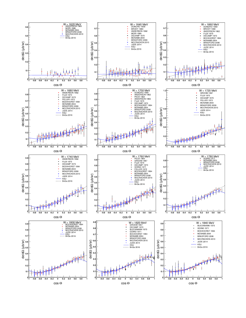
Figure 8: Fits to $\frac{d\sigma}{d\Omega}$ for $\gamma p\rightarrow K^{+}\Lambda$ at $W$ = 1620 to 1840 MeV. See text for references.

Figure 9: Fits to $\frac{d\sigma}{d\Omega}$ for $\gamma p\rightarrow K^{+}\Lambda$ at $W$ = 1870 to 2230 MeV. See text for references.

Figure 10: Fits to $\Sigma$ for $\gamma p\rightarrow K^{+}\Lambda$ at $W$ = 1640 to 1910 MeV. See text for references.

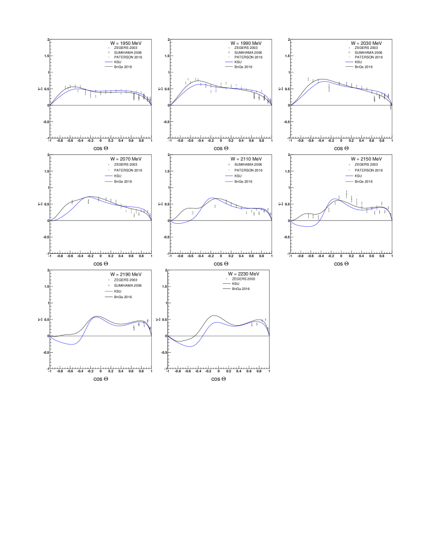
Figure 11: Fits to $\Sigma$ for $\gamma p\rightarrow K^{+}\Lambda$ at $W$ = 1950 to 2230 MeV. See text for references.

Figure 12: Fits to $T$ for $\gamma p\rightarrow K^{+}\Lambda$ at $W$ = 1640 to 1840 MeV. See text for references.

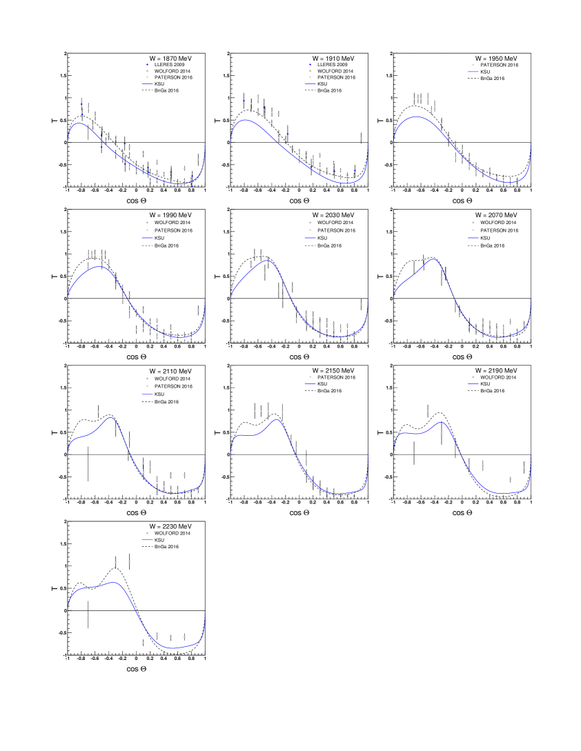
Figure 13: Fits to $T$ for $\gamma p\rightarrow K^{+}\Lambda$ at $W$ = 1870 to 2230 MeV. See text for references.

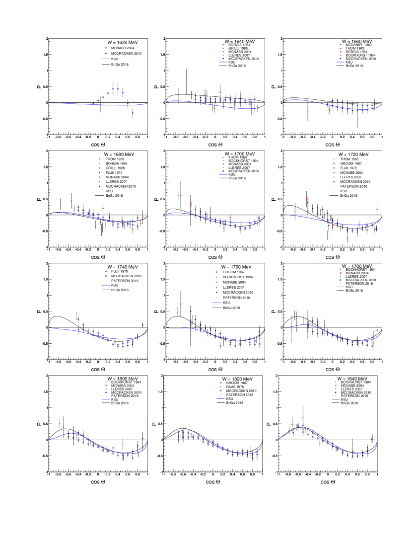
Figure 14: Fits to $P$ for $\gamma p\rightarrow K^{+}\Lambda$ at $W$ = 1620 to 1840 MeV. See text for references.

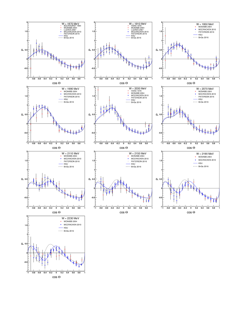
Figure 15: Fits to $P$ for $\gamma p\rightarrow K^{+}\Lambda$ at $W$ = 1870 to 2230 MeV. See text for references.

Figure 16: Fits to $E$ for $\gamma p\rightarrow K^{+}\Lambda$ at $W$ = 1680 to 2110 MeV. See text for references.

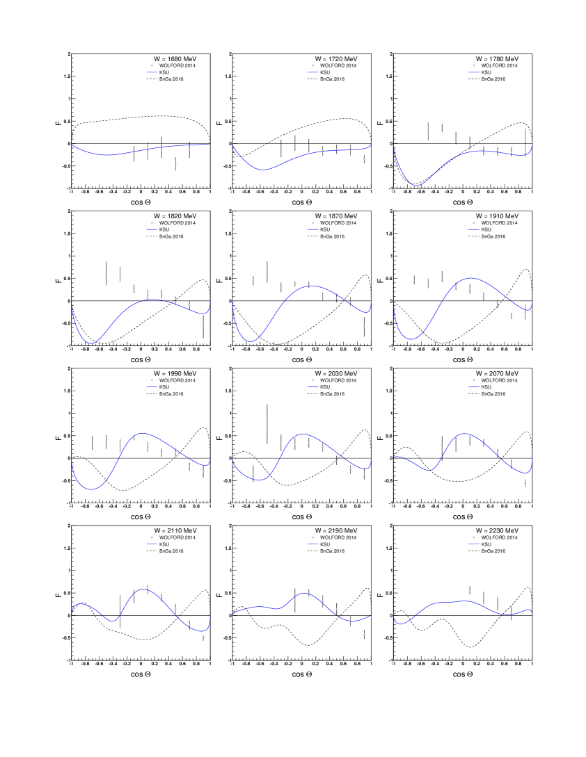
Figure 17: Fits to $F$ for $\gamma p\rightarrow K^{+}\Lambda$ at $W$ = 1680 to 2230 MeV. See text for references.

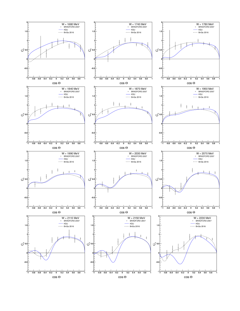
Figure 18: Fits to $C_{x}$ for $\gamma p\rightarrow K^{+}\Lambda$ at $W$ = 1680 to 2230 MeV. See text for references.

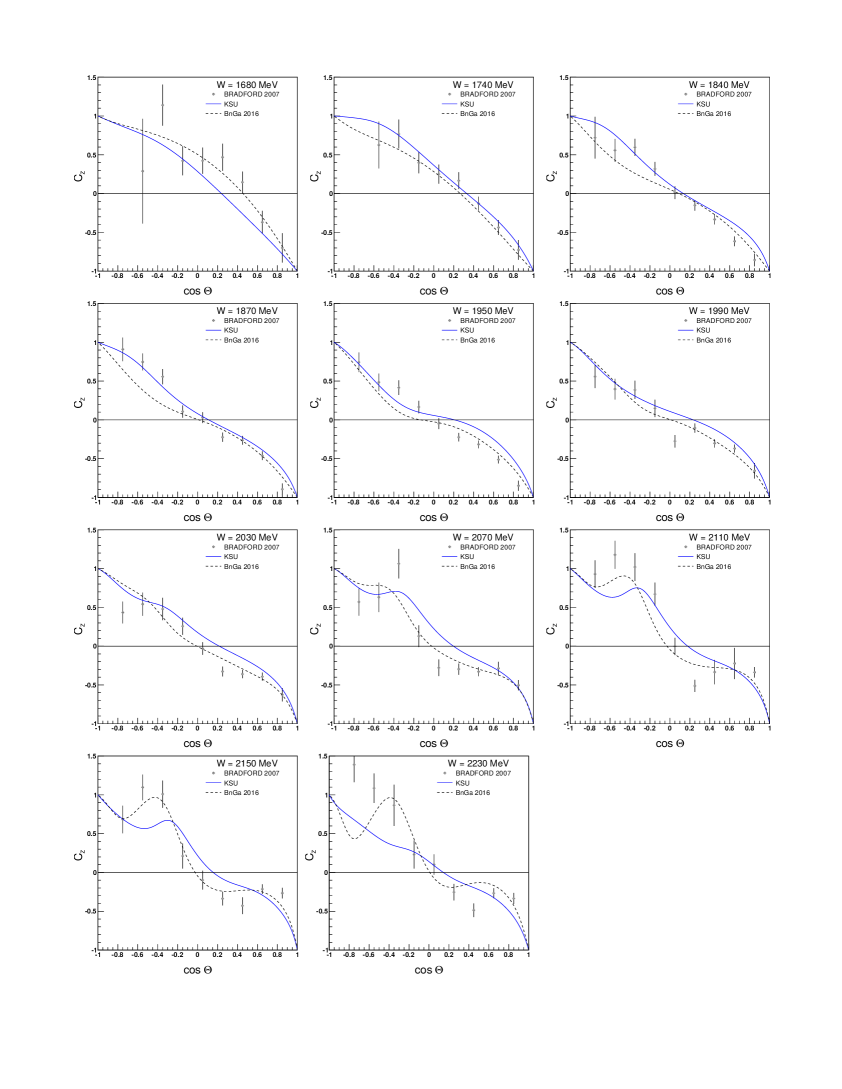
Figure 19: Fits to $C_{z}$ for $\gamma p\rightarrow K^{+}\Lambda$ at $W$ = 1680 to 2230 MeV. See text for references.

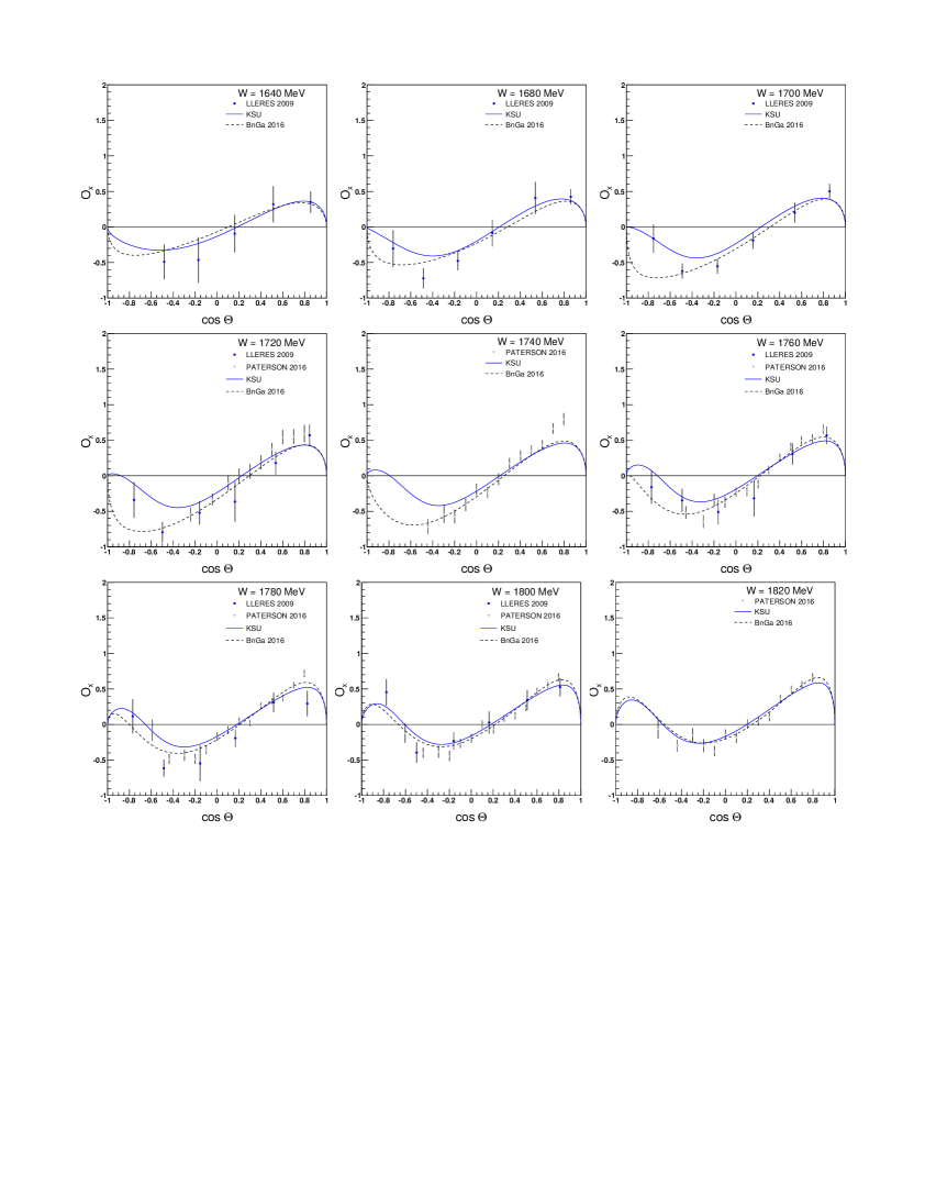
Figure 20: Fits to $O_{x}$ for $\gamma p\rightarrow K^{+}\Lambda$ at $W$ = 1640 to 1820 MeV. See text for references.

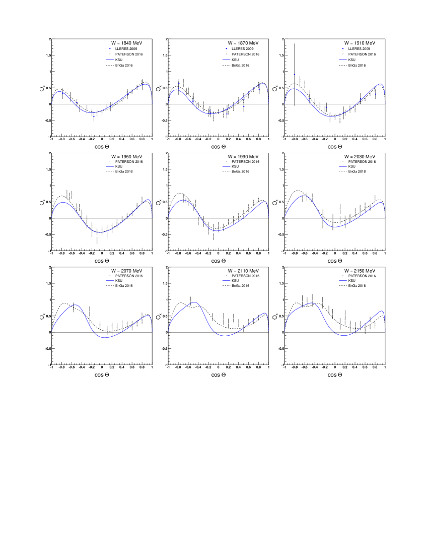
Figure 21: Fits to $O_{x}$ for $\gamma p\rightarrow K^{+}\Lambda$ at $W$ = 1840 to 2150 MeV. See text for references.

Figure 22: Fits to $O_{z}$ for $\gamma p\rightarrow K^{+}\Lambda$ at $W$ = 1640 to 1820 MeV. See text for references.

Figure 23: Fits to $O_{z}$ for $\gamma p\rightarrow K^{+}\Lambda$ at $W$ = 1840 to 2150 MeV. See text for references.

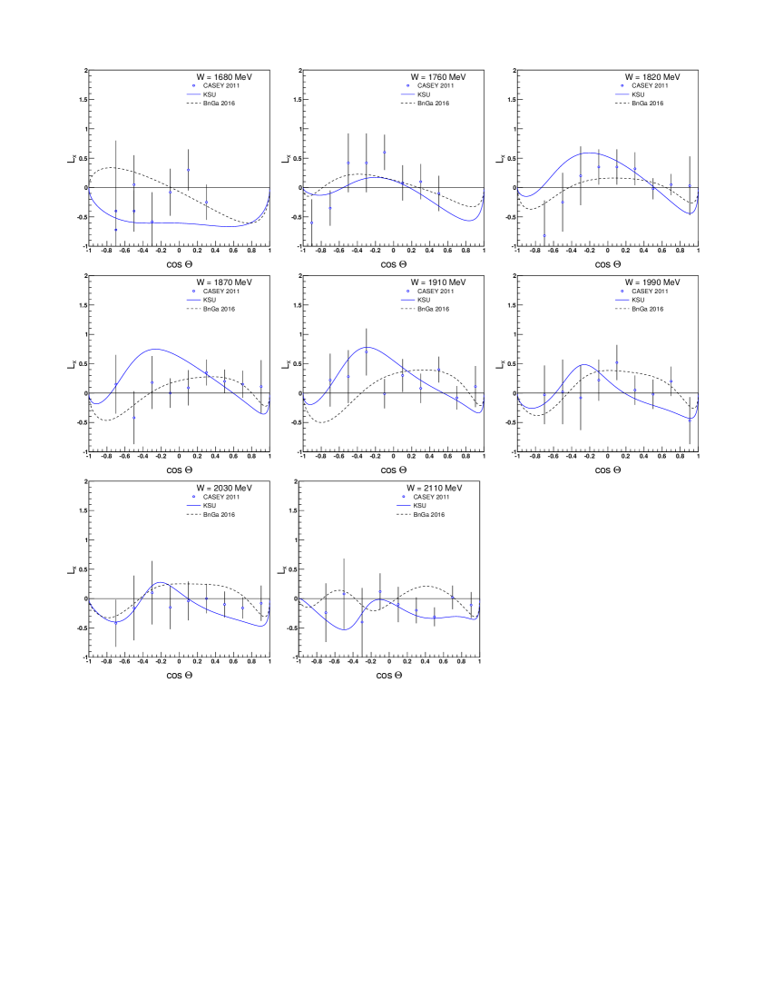
Figure 24: Fits to $L_{x}$ for $\gamma p\rightarrow K^{+}\Lambda$ at $W$ = 1680 to 2110 MeV. See text for references.

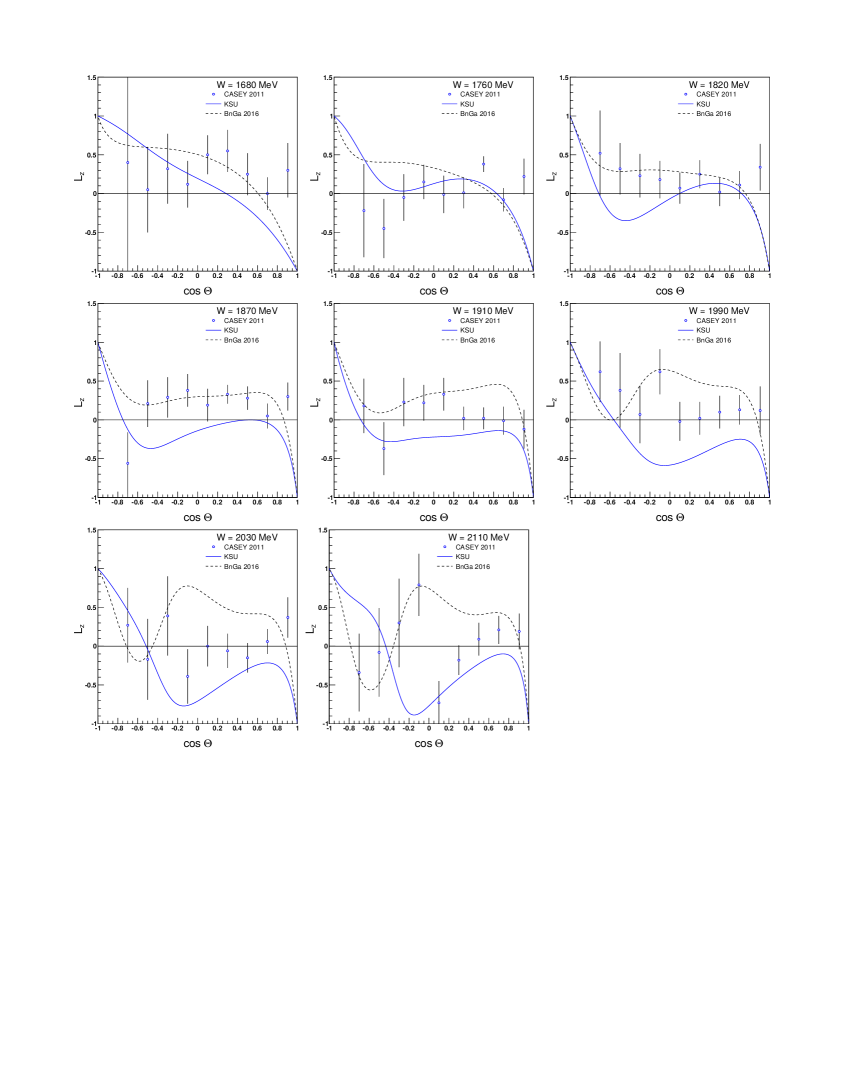
Figure 25: Fits to $L_{z}$ for $\gamma p\rightarrow K^{+}\Lambda$ at $W$ = 1680 to 2110 MeV. See text for references.

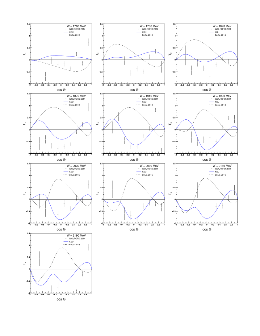
Figure 26: Fits to $T_{x}$ for $\gamma p\rightarrow K^{+}\Lambda$ at $W$ = 1700 to 2190 MeV. See text for references.

Figure 27: Fits to $T_{z}$ for $\gamma p\rightarrow K^{+}\Lambda$ at $W$ = 1740 to 2150 MeV. See text for references.