Lagrangian geography of the deep Gulf of Mexico

Abstract

Using trajectories from acoustically tracked (RAFOS) floats in the Gulf of Mexico, we construct a geography of its Lagrangian circulation within the 1500–2500-m layer. This is done by building a Markov-chain representation of the Lagrangian dynamics. The geography is composed of weakly interacting provinces that constrain the connectivity at depth. The main geography includes two provinces of near equal areas and separated by a roughly meridional boundary. The residence time is about 4.5 (3.5) years in the western (eastern) province. The exchange between these provinces is effected through a slow cyclonic circulation, which is well constrained in the western basin by preservation of $f/H$, where $f$ is the Coriolis parameter and $H$ is depth. Secondary provinces of varied shapes covering smaller areas are identified with residence times ranging from about 0.4 to 1.2 years or so. Except for the main provinces, the deep Lagrangian geography does not resemble the surface Lagrangian geography recently inferred from satellite-tracked drifter trajectories. This implies disparate connectivity characteristics with potential implications for pollutant (e.g., oil) dispersal at the surface and depth. A ventilation conduit through the southeastern corner of the domain from the Caribbean Sea balanced by weak vertical exchange is also inferred. This is supported by the inspection of satellite-tracked profiling (Argo) floats, which, while forming a smaller dataset and having seemingly different water-following characteristics than the RAFOS floats, replicate the main aspects of the Lagrangian geography. Finally, consistency with independent results from a chemical tracer release experiment is found to provide additional support to the results.

1 Introduction

The oil spill produced by the Deepwater Horizon drilling rig explosion in May 2010 (Lubchenco et al. 2012) has motivated great interest in the Lagrangian circulation of the Gulf of Mexico (GoM). This is reflected in the execution in recent years of a number of field campaigns dedicated to observe its surface Lagrangian circulation. A main reason for investigating the surface Lagrangian circulation is found in the very tangible effects it had on the evolution of the oil slick that emerged from the ocean floor (Olascoaga and Haller 2012). The main campaigns have been the Grand LAgrangian Deployment (GLAD) in July 2012 (Olascoaga et al. 2013; Poje et al. 2014; Beron-Vera and LaCasce 2016) and the LAgrangian Submesoscale ExpeRiment (LASER) in February 2016 (Miron et al. 2017; Novelli et al. 2017). These two campaigns contributed to nearly duplicate the satellite-tracked surface drifter database existing prior to the oil spill, which consisted mainly of drifter trajectories from the National Oceanic and Atmospheric Administration (NOAA) Global Drifter Program (GDP, Lumpkin and Pazos 2007) and the Surface Current Lagrangian-Drifter Program (SCULP, Sturgers et al. 2001; Ohlmann and Niiler 2005), see Miron et al. (2017) for details.

Large amounts of oil were reported to stay submerged and to persist for months without substantial biodegradation (Camilli et al. 2010). Yet the effects that the deep Lagrangian circulation had on the submerged oil remained elusive, which directly or indirectly motivated the execution of experiments to also observe the Lagrangian circulation at depth. One experiment consisted in a deployment of acoustically tracked floats in a mission that started in 2011 and lasted out to 2015 (Hamilton et al. 2016). This contributed to augment the existing submerged float database, consisting mainly of profiling floats from a dedicated experiment (Weatherly et al. 2005) and routine sensing of the deep global ocean (Roemmich et al. 2009). Another experiment involved the release of a chemical tracer at depth in July 2012 near the Deepwater Horizon site and its subsequent sampling over the course of one year (Ledwell et al. 2016).

An aspect of the deep Lagrangian circulation highlighted by the dedicated profiling float experiment (Weatherly et al. 2005) was the restricted communication between the eastern and western GoM basins and also a cyclonic circulation at about 900 m in the southwestern sector. Analysis of the acoustically tracked float trajectories in the western basin (Pérez-Brunius et al. 2017) from the recent experiment (Hamilton et al. 2016) further revealed the existence of a cyclonic boundary current below 900 m and a cyclonic gyre in the abyssal plain consistent with numerical studies (Oey and Lee 2002), and the analysis of hydrographic data (DeHaan and Sturges 2005) and deep-water moorings (Tenreiro et al. 2018). Direct inspection of the same acoustically tracked float trajectories (Pérez-Brunius et al. 2017), as well as rough estimates of connectivity between the eastern and western basins (Hamilton et al. 2016), suggests that the exchange between them occurs along the boundary following a cyclonic circulatory motion. In turn, the analysis of the dispersion of the chemical tracer released at depth in the eastern basin (Ledwell et al. 2016) concluded that homogenization by stirring and mixing is substantially faster in the GoM than in the open ocean. The main source of energy in the deep eastern basin is presumably provided by the Loop Current by inducing a deep flow through baroclinic instabilities, deep eddies, and topographic Rossby waves which can transfer energy toward the western basin (Sheinbaum et al. 2016; Hamilton et al. 2016; Donohue et al. 2016).

The goal of this paper is to shed new light on the deep Lagrangian circulation in the GoM by using probabilistic tools from nonlinear dynamical systems. These are applied on the above acoustically tracked float trajectories with a focus on connectivity. Investigating connectivity with the probabilistic nonlinear dynamics tools boils down to analyzing the eigenvectors of a transfer operator approximated by a matrix of probabilities of transitioning between boxes of a grid, which provides a discrete representation of the Lagrangian dynamics (Froyland et al. 2014). Markov-chain representations of this type had originally been used to approximate almost-invariant sets in nonlinear dynamical systems using short-run trajectories (Hsu 1987; Dellnitz and Junge 1999; Froyland 2005), and in the ocean context to determine the extent of Antarctic gyres in 2- (Froyland et al. 2007) and 3-space (Dellnitz et al. 2009) dimensions. This eigenvector method has been recently applied on drifter data to construct a geography of the surface Lagrangian circulation (Miron et al. 2017). A Lagrangian geography is composed of dynamical provinces that delineate weakly interacting basins of attraction for almost-invariant attractors, which imposes constraints on connectivity. Here we construct a geography for the deep Lagrangian circulation, providing firm support to earlier inferences from the direct inspection float trajectories and, furthermore, revealing a number of aspects transparent to traditional Lagrangian data analysis.

2 Data

The main dataset analyzed in this paper is composed of trajectories produced by a total of 154 quasi-isobaric acoustically tracked RAFOS (SOund Fixing And Ranging or SOFAR, spelled backward) floats (Rossby et al. 1986) deployed in the GoM (Hamilton et al. 2016). Starting in 2011, 121 floats ballasted for 1500 m and 31 floats for a lower depth of 2500 m were deployed in the following 2 years. Each float recorded position fixes 3 times daily, with record lengths varying between 7 days and 1.5 years. This sampling is too frequent for an estimated uncertainty of the order of 5 km, so we here consider daily interpolated trajectories. The float deployment during the first 2 years of a 4-year-long program was performed by several U.S. (Woods Hole Oceanographic Institution, Leidos Corporation, University of Colorado) and Mexican (Centro de Investigación Científica y de Educación Superior de Ensenada) teams sponsored by the U.S. Bureau of Ocean Energy Management (BOEM). The records of the last floats deployed ended in summer 2015. The recorded trajectories of all floats are shown in Fig. 1 (deployment locations and final positions are indicated in blue and red, respectively). The trajectories cover a region bounded for the most part by the 1750-m isobath (dashed lines in Fig. 1 indicate, from outside to inside, the 1500-, 1750-, and 2500-m isobaths). Note that while the floats are too deep to escape the GoM through the Straits of Florida (where the maximum depth is roughly 700 m), they are capable of escaping through the Yucatan Channel (where the maximum depth is about 2000 m). Mooring measurements suggest that the latter is indeed possible as they have revealed a countercurrent between 500 and 1750 m on the western and eastern sides of the Yucatan Channel (Sheinbaum et al. 2002). However, no float is seen to travel into the Caribbean Sea. Confinement of the 1500- and 1750-m floats within the region bounded by the 1750-m isobath suggests predominantly columnar motion. This is confirmed by the analysis presented below, which ignores the depth of the floats to maximize the number of available trajectories.

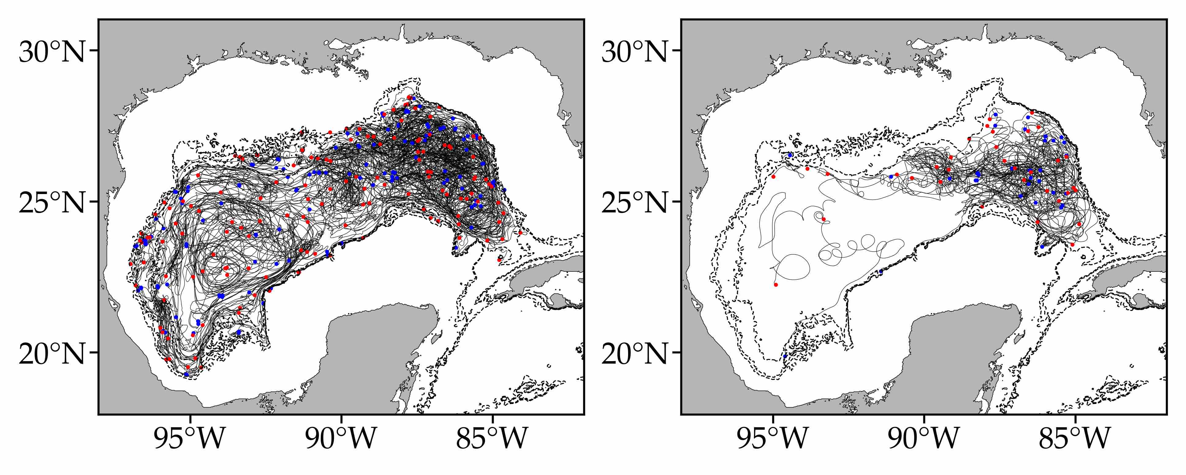
Figure 1: Trajectories of RAFOS floats ballasted at 1500 (left) and 2500 (right) m in the Gulf of Mexico over 2011–2015. Indicated are initial (blue dots) and final (red dots) positions of the floats. The dash lines indicate, from outside to inside, the 1500-, 1750-, and 2500-m isobaths.

We also analyze trajectories recorded by all available (60) profiling floats in the GoM from the Argo Program (Roemmich et al. 2009). Unlike RAFOS float positions, Argo float positions are recorded every 10 days after the float descends down to a parking depth of 1000 m, where it drifts for 9 days, and further to 2000 m to begin profiling temperature and salinity in its ascend back to the surface. The trajectories of the Argo floats roughly sample the same area as the RAFOS floats albeit much less densely. However, the way that the Argo floats sample the deep Lagrangian circulation may be expected to differ from the way done it by the RAFOS floats, which remain at all times parked at a fixed depth. Despite this expectation, we show that Argo floats replicate some important aspects of the deep circulation inferred using the RAFOS floats.

A third set of independent data considered is composed of concentrations of chemical tracer from a release experiment (Ledwell et al. 2016). In the experiment, a 25-km-long streak of CF₃SF₅ was injected on an isopycnal surface about 1100-m deep and 150 m above the bottom, along the continental slope of the northern GoM, about 100-km southwest of the Deepwater Horizon oil well, where oil was detected at depth after its explosion. The tracer was sampled between 5 and 12 days after release, and again 4 and 12 months after release.

3 Theory

3.1 Transfer operator and transition matrix

Let $X\in\mathbb{R}^{2}$ be a closed flow domain on the plane. We assume that the Lagrangian dynamics is governed by an advection–diffusion process. A tracer initialized at position $y\in X$ (represented by a delta-measure $\delta_{y}$) therefore evolves passively $T>0$ units of time to a probability density $K(x,y)$, with $x\in X$. The function $K(x,y)$ is clearly nonnegative, and we normalize in $x$ so that

$$\smash{\int_{X}K(x,y)\,dx=1}.$$ (1)

The function $K(x,y)$ is a (bounded) stochastic kernel; cf., e.g., Sections 5.7 and 11.7 of Lasota and Mackey (1994) for a discussion of stochastic kernels and advection–diffusion equations, respectively. To evolve a general initial density $h:X\to\mathbb{R}^{+}$ forward $T$ units of time, we define a Markov operator, known as the Perron-Frobenius operator, or more generally a transfer operator, $\mathcal{P}:L^{1}(X)\circlearrowleft$, as

$$\mathcal{P}h(x)=\int_{X}K(x,y)h(y)\,dy.$$ (2)

The density $\mathcal{P}h(x)$ is the result of evolving $h(x)$ forward $T$ units of time under the advection–diffusion dynamics.

Note that the only time dependence is the duration of time $T$. In particular, we do not model variation of the advection–diffusion dynamics as a function of initial time. This is appropriate for a probabilistic description of the dynamics, as done in statistically stationary turbulence (Orszag 1977), yet it is also a consequence of the nature of the dataset considered here. In either case the significance of the time homogeneity assumption can only be assessed a posteriori, as we do here.

A discretization of the transfer operator can be attained using a Galerkin approximation referred to as Ulam’s method (Ulam 1979; Kovács and Tél 1989). This involves partitioning the domain $X$ into a grid of $N$ connected boxes $\smash{\{B_{1},\dotsc,B_{N}\}}$ and projecting functions in $L^{1}(X)$ onto the finite-dimensional approximation space $\smash{V_{N}:=\mbox{span}\{\mathbf{1}_{B_{1}}(x),\dotsc,\mathbf{1}_{B_{N}}(x)\}}$, where $\mathbf{1}_{B_{i}}(x)=1$ for $x\in B_{i}$ and 0 otherwise is the indicator function of set $B_{i}$. Define $\pi_{N}:L^{1}(X)\to V_{N}$ by

$$\smash{\pi_{N}h(x)}=\sum_{j=1}^{N}\frac{\int_{B_{j}}h(x)\,dx}{\operatorname{area}(B_{j})}\,\mathbf{1}_{B_{j}}(x).$$ (3)

To calculate the projected action of $\mathcal{P}$ on $V_{N}$ we compute:

$$\pi_{N}\mathcal{P}\mathbf{1}_{B_{i}}(x)\!\!\!\! = \!\!\!\!\sum_{j=1}^{N}\frac{\int_{B_{j}}\mathcal{P}\mathbf{1}_{B_{i}}(x)\,dx}{\operatorname{area}(B_{j})}\,\mathbf{1}_{B_{j}}(x)$$ (4)

$$= \!\!\!\!\sum_{j=1}^{N}\frac{\int_{B_{j}}\int_{X}K(x,y)\mathbf{1}_{B_{i}}(y)\,dydx}{\operatorname{area}(B_{j})}\,\mathbf{1}_{B_{j}}(x)$$

$$= \!\!\!\!\sum_{j=1}^{N}\underbrace{\frac{\int_{B_{j}}\int_{B_{i}}K(x,y)\,dydx}{\operatorname{area}(B_{j})}}_{=:P_{ij}}\,\mathbf{1}_{B_{j}}(x)$$

The $(i,j)$-th entry of the array $P_{ij}$ represents an approximation of the kernel $K(x,y)$ for $y\in B_{i},x\in B_{j}$. We assume from now on that the grid is regular, i.e., $\operatorname{area}(B_{i})=\operatorname{area}(B_{j})$ for all $1\leq i,j\leq N$. Because $K(x,y)$ represents the density obtained by evolving $\delta_{y}$ forward $T$ units of time,

$$P_{ij}=\frac{\int_{B_{j}}\int_{B_{i}}K(x,y)\,dydx}{\operatorname{area}(B_{i})}$$ (5)

is the proportion of tracer beginning in $B_{i}$ that is found in $B_{j}$ after $T$ units of time (“proportion” because of integration over $B_{j}$ and the property (1)), averaged over the initial tracer in $B_{i}$ (“averaged” because of the integration over $B_{i}$ and division by $\operatorname{area}(B_{i})$).

If we are presented with tracer data in the form of trajectories of individual tracer particles, by considering a sufficiently large number of particles over a total time horizon $[0,\mathcal{T}]$ we can estimate the entries of $P_{ij}$ as

$$P_{ij}\approx\frac{\mbox{\# $x\in B_{i}$ at $t\in[0,\mathcal{T}-T]$ and $B_{j}$ at $t+T$}}{\mbox{\# $x\in B_{i}$ at $t\in[0,\mathcal{T}-T]$}}.$$ (6)

The transition matrix $\smash{P\in\mathbb{R}^{N\times N}}$ defines a Markov-chain representation of the dynamics, with the entries $P_{ij}$ equal to the conditional transition probabilities between boxes, which are represented by the states of the chain.

The forward evolution of the discrete representation of $h(x)$, $\mathbf{h}=(h_{1}\,\cdots\,h_{N})$, is calculated under left multiplication, i.e.,

$$\mathbf{h}^{(k)}=\mathbf{h}P^{k},\quad k=1,2,\dotsc.$$ (7)

We note that the discrete evolution described by $P$ introduces additional diffusion with magnitude of the order of the box diameters (Froyland 2013).

3.2 Ergodicity, mixing, attracting sets, residence time, and retention time

Because the transition matrix $P$ is row stochastic, i.e., $\smash{\sum_{j=1}^{N}P_{ij}}=1\ \forall i$, $\mathbf{1}=(1\dotsb 1)$ is a right eigenvector with eigenvalue $\lambda=1$, i.e., $P\mathbf{1}=\mathbf{1}$. The eigenvalue $\lambda=1$ equals the spectral radius of $P$. The associated nonunique left eigenvector $p$ is normalized to a probability vector ($\smash{\sum_{i=1}^{N}p_{i}=1}$) which is invariant (because $pP=p$) and nonnegative (by the Perron–Frobenius theorem, Horn and Johnson 1990).

We call $P$ irreducible (or ergodic) if for each $1\leq i,j\leq N$ there is an $n_{ij}<\infty$ such that $\smash{(P^{n_{ij}})_{ij}>0}$. All states of an irreducible Markov chain communicate, the eigenvalue $\lambda=1$ is simple, and the corresponding left eigenvector $p$ is strictly positive (Horn and Johnson 1990). We call $P$ aperiodic (or mixing) if there is an $i$ such that $\gcd\{n\geq 0\mid\smash{(P^{n})_{ii}>0}\}=1$. For aperiodic $P$ one has $\smash{p=\lim_{k\to\infty}\mathbf{h}P^{k}}$ for any initial probability vector $\mathbf{h}$.

Suppose that $P$ is irreducible on some class of states $S\subset\{1,\dotsc,N\}$. We call $S$ an absorbing closed communicating class if $P_{ij}=0$ for all $i\in S,j\notin S$, and $P_{ij}>0$ for some $i\notin S,j\in S$; cf. Froyland et al. (2014). The set $\smash{B_{S}=\bigcup_{i\in S}B_{i}\subset X}$ forms an approximate time-asymptotic forward-invariant attracting set for trajectories starting in $\smash{X=\bigcup_{i=1}^{N}B_{i}}$.

Markov chain theory also provides a very simple means of determining the mean residence time in a collection of boxes. For $A\subset X$ let $P|_{A}$ be the transition matrix $P$ restricted to the subset of indices corresponding to boxes whose union is $A$. The mean time $\tau_{i}$ of a trajectory initialized in box $B_{i}$ to move out of $A$, also known as the mean time to hit the complement of $A$, is given by the solution of the linear equation (cf., e.g., Norris (1998) and Dellnitz et al. (2009) for its use in the context of ocean dynamics):

$$(\operatorname{Id}-P|_{A})\tau/T=\mathbf{1},$$ (8)

where $\operatorname{Id}$ is the identity matrix. The mean value of $\tau$ within $A$ is a measure of the residence time of the entire set.

Another timescale related to residence time is the time-asymptotic retention time. As before, let $A\subsetneq X$ be the set for which we wish to allocate a retention time and denote $P|_{A}$ the restriction of $P$ to boxes whose union is $A$. If $P$ is mixing, the leading positive eigenvalue of $P|_{A}$, $\lambda_{A}$, is strictly less than 1. If one conditions on the fact that trajectories have already remained in $A$ sufficiently long (so they are distributed like $p_{A}\geq 0$, the leading left eigenvector of $P|_{A}$), then the probability of remaining in $A$ for one more application of $P$ is $\lambda_{A}$. The probability of a point in $A$ (distributed according to $p_{A}$) remaining in $A$ for $k\geq 1$ applications of $P$ is

$$\frac{\lambda_{A}^{k}}{\sum_{k=1}^{\infty}\lambda_{A}^{k}}=\frac{\lambda_{A}^{k}}{\lambda_{A}/(1-\lambda_{A})}=(1-\lambda_{A})\lambda_{A}^{k-1}.$$ (9)

Hence, the mean retention time $\mathfrak{T}$ for points in $A$ distributed according to $p_{A}$ is

$$\mathfrak{T}/T = \sum_{k=1}^{\infty}\left((1-\lambda_{A})\lambda_{A}^{k-1}\right)\cdot k$$ (10)

$$= (1-\lambda_{A})\sum_{k=1}^{\infty}k\lambda_{A}^{k-1}$$

$$= (1-\lambda_{A})\cdot\frac{1}{(1-\lambda_{A})^{2}}$$

$$= \frac{1}{1-\lambda_{A}}.$$

Note that if the mean value of $\tau$, $\tau_{A}$, is computed according to $p_{A}$, i.e., $\tau_{A}=\sum_{j\in A}(p_{A})_{j}\tau_{j}$, then $\tau_{A}=\mathfrak{T}$.

3.3 Lagrangian geography from almost-invariant decomposition

Revealing those regions in which trajectories tend to stay for a long time before entering another region is key to assessing connectivity in a flow. Such forward time-asymptotic almost-invariant sets and their corresponding backward-time basins of attraction can be framed (Froyland et al. 2014) by inspecting eigenvectors of $P$ with $\lambda\approx 1$.

The magnitude of the eigenvalues quantify the geometric rates at which eigenvectors decay. Those left eigenvectors with $\lambda$ closest to 1 are the slowest to decay and thus represent the most long-lived transient modes (Froyland 1997; Pikovsky and Popovych 2003). For a given $\lambda\approx 1$, a forward time-asymptotic almost-invariant set will be identified with the support of similarly valued and like-sign elements in the left eigenvector. Regions where the magnitude of the left eigenvector is greatest are the most dynamically disconnected and take the longest times to transit to other almost-invariant sets.

The multiple backward-time basins of attraction are identified by boxes where the corresponding right eigenvectors take approximately constant values (cf. Koltai 2011, for the simpler single basin case). Decomposition of the ocean flow into weakly disjoint basins of attraction for time-asymptotic almost-invariant attracting sets using the above eigenvector method has been shown (Froyland et al. 2014; Miron et al. 2017) to form the basis of a Lagrangian geography of the ocean, where the boundaries between basins are determined from the Lagrangian circulation itself, rather than from arbitrary geographical divisions.

We note that the eigenvector method differs from the flow network approach (Rossi et al. 2014; Ser-Giacomi et al. 2015). The eigenvector method analyzes time-asymptotic aspects of the dynamics through spectral information from the generating Markov chain, while the flow network approach computes various graph-based quantities for finite-time durations to study flow dynamics.

4 Results

4.1 Building a Markov-chain model

To discretize the deep-ocean Lagrangian dynamics in the GoM, we laid down on the region $X$ spanned by the trajectories of the RAFOS floats in Fig. 1 a grid with $N=946$ boxes of roughly 25-km a side. The size of the boxes was selected to maximize the grid’s resolution while each individual box is sampled by enough trajectories (recall that the float’s position is determined with a precision of about 5 km, so the uncertainty area around a float’s location is roughly 8 times smaller than the area of a box in the grid). Figure 2 shows number of floats per box in the grid, independent of time over the entire 2011–2015 period (left) and within each season in this period (right). Regions not visited by floats are found in each season, particularly in winter. Ignoring time, there are on average 86 floats per box, with 1 box having as many as 286 floats and 7 boxes only 1 float. Overall, while the float coverage may not be dense enough to carry out a seasonal analysis, it is sufficient in space to build a Markov-chain model that assumes time homogeneity (Maximenko et al. 2012; van Sebille et al. 2012; Miron et al. 2017; McAdam and van Sebille 2018).

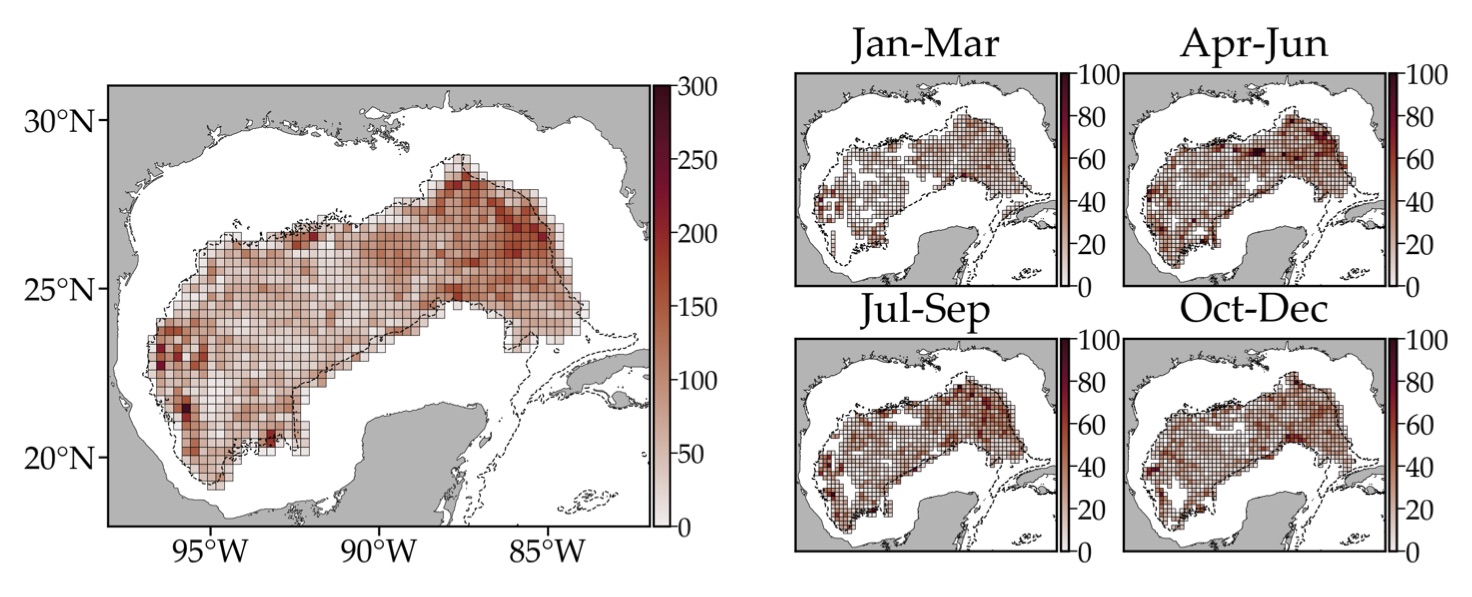
Figure 2: For daily interpolated trajectories, number of RAFOS floats per box in the grid into which the domain visited has been discretized, independent of time over the entire 2011–2015 period (left) and within each season in this period (right). The dashed line, here and all the subsequent figures, represent the 1750-m isobath.

Before getting into the specifics of the computation of the transition matrix $P$ defining the Markov chain, it is important to note that formula (5) for $P$ does not require the number of trajectories that sample the boxes in the partition to be equal for each box. Thus the nonuniform sampling of the RAFOS floats is not an impediment for computing $P$. Nevertheless, to make sure that this does not introduce any biases in our analysis, we have also computed various $P$s by randomly choosing a fixed number (50) of trajectories. This required us to eliminate 94 boxes from the original partition. The resulting $P$s were found to produce results that could not be distinguished from those produced by the $P$ computed using all available trajectories, as done as follows.

Using formula (6), we computed the $P_{ij}$ entry of the transition matrix by counting the number of floats that starting in box $B_{i}$ on any day landed in box $B_{j}$ after $T=7$ days within the entire record of float data, which lasts $\mathcal{T}\approx 4$ years. A transition time $T=7$ days in general guarantees interbox communication. Furthermore, $T=7$ days is larger than the Lagrangian decorrelation timescale, which we estimated to be of about 5 days for half decorrelation consistent with earlier estimates (cf. LaCasce 2008). Markovian dynamics can be expected to approximately hold as there is negligible memory farther than 7 days into the past. A similar reasoning was applied in applications involving surface drifters (Maximenko et al. 2012; van Sebille et al. 2012; Miron et al. 2017; McAdam and van Sebille 2018), in which case the transition time was taken shorter due to the shorter decorrelation time near the ocean surface (LaCasce 2008). The results presented below were found insensitive to variations of $T$ in the range 7–21 days.

4.2 Assessing communication within the Markov chain

A Markov chain can be seen as a directed graph with vertices corresponding to states in the chain, and directed arcs corresponding to one-step transitions of positive probability. This allows one to apply Tarjan’s algorithm (Tarjan 1972) to assess communication within a chain. Specifically, the Tarjan algorithm takes such a graph as input and produces a partition of the graph’s vertices into the graph’s strongly connected components. A directed graph is strongly connected if there is a path between all pairs of vertices. A strongly connected component of a directed graph is a maximal strongly connected subgraph and by definition also a maximal communicating class of the underlying Markov chain.

Applying the Tarjan algorithm to the directed graph associated with the Markov chain derived using the float trajectory data, we found a total of four maximal communicating classes. Each one of these classes is indicated with a different color in Fig. 3. One class, denoted $S_{\mathrm{L}}$, is large, composed of the majority of the states in the chain or boxes of the partition (935 out of a total of $N=946$). From direct computation, $P_{ij}=0$ for all $i\in S_{\mathrm{L}}$, $j\notin S_{\mathrm{L}}$, i.e., $S_{\mathrm{L}}$ is closed. The classes in the complement of $S_{\mathrm{L}}$ are small, with 2 formed by a single state and another one formed by 9 states. Direct computation shows that $(P^{m})_{ij}>0$ for some $m$ for all $i\notin S_{\mathrm{L}}$, $j\notin S_{\mathrm{L}}$. This reveals that $S_{\mathrm{L}}$ is absorbing. Because $S_{\mathrm{L}}$ is communicating and closed, $P$ restricted to $S_{\mathrm{L}}$, i.e., $P|_{S_{\mathrm{L}}}$, is irreducible and provided that no state repeatedly occurs, it will be mixing, i.e., a unique, limiting invariant probability density will be supported on $S_{\mathrm{L}}$. Because $S_{\mathrm{L}}$ is absorbing, its small complement can be safely ignored from the analysis without affecting the results by replacing $P$ with $P|_{S_{\mathrm{L}}}$.

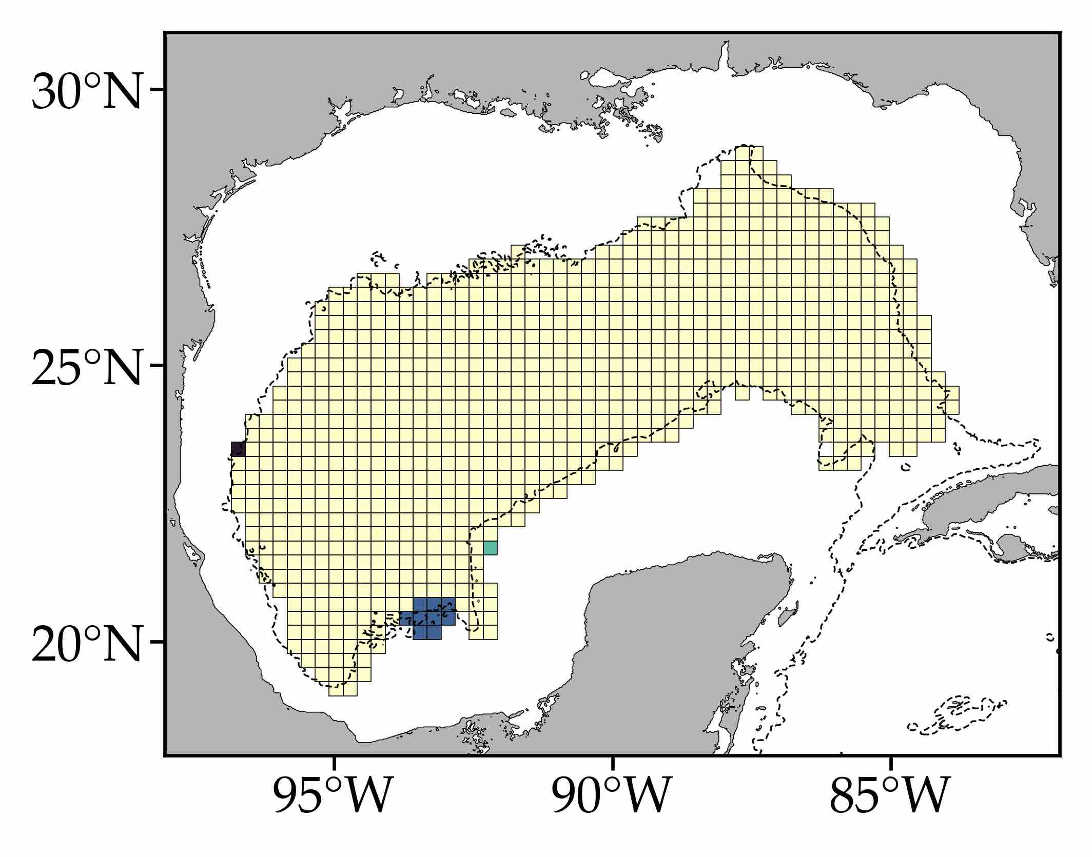
Figure 3: Grouping of the states of the Markov chain associated with the matrix $P$ of transition probabilities of RAFOS floats moving over 7 days between boxes of the partition of the domain spanned by their trajectories into classes according to their communication type. Boxes indicated with the same color belong to the same class. There are 4 maximal communicating classes, with a large class (yellow) encompassing most of the states in the Markov chain (boxes of the partition) which is absorbing.

4.3 Forward evolution of the probability density of a tracer

Figure 4 shows selected snapshots of the push forward of the probability density of a tracer initially uniformly distributed within the layer between 1500 and 2500 m in the GoM under the discrete action of the underlying flow map. At the coarse-grained level given by the grid defined above, this is defined by (7) with $\mathbf{h}=\mathbf{1}/N$ and $P$ as derived using the float data. Because we used 7-day-long trajectory pieces to construct $P$, one application of $P$ is equivalent to evolving in forward time for $T=7$ d. Note that the density eventually settles on a nonuniform distribution which appears to be invariant.

The regions where the density distribution of Fig. 4 locally maximizes represent vertical “outwelling” sites. Likewise, there is vertical “inwelling” in the regions where the density locally minimizes. Volume conservation in either case implies vertical motion. While the direction of this motion cannot be determined from the analysis of the float trajectories on a single layer, some sense may be made of its magnitude by comparing area change estimates obtained using the deep floats and the satellite-tracked surface drifter data employed in Miron et al. (2017).

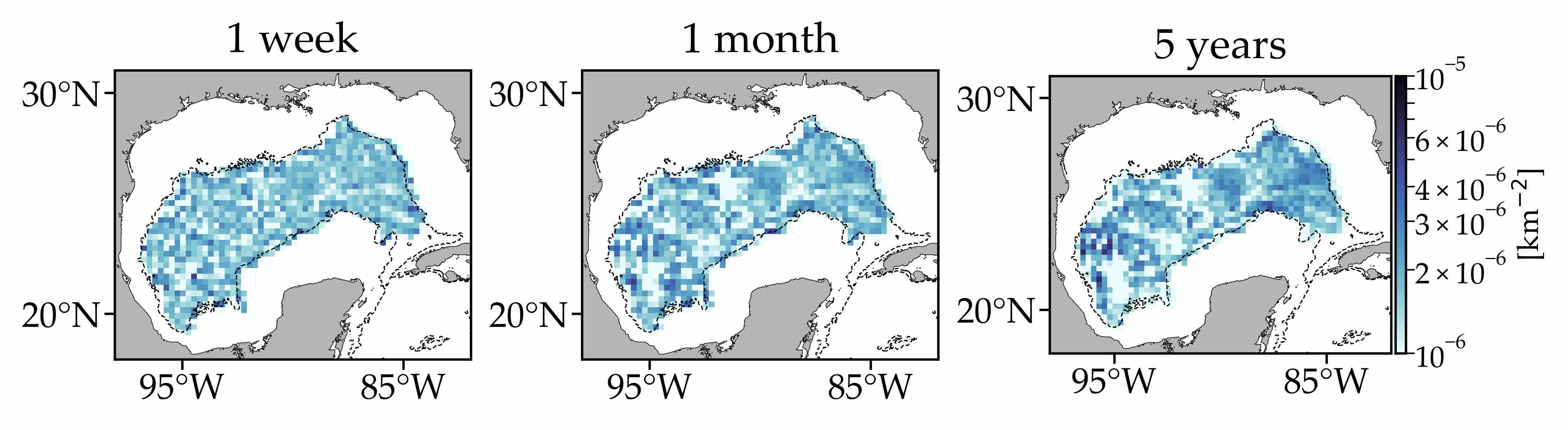
Figure 4: Selected snapshots of the evolution of an initially uniformly distributed tracer probability density under the action of the underlying flow map, whose discrete representation is provided by the float-data-derived transition matrix $P$.

Let $a_{i}$ be the area of box $B_{i}$ of the domain on which the float trajectories lie. After 1 application of $P$, equivalently 7 d, we have $a^{\prime}_{i}:=\smash{\sum_{j=1}^{N}a_{j}P_{ji}}$. If the flow were area-preserving, we would expect $a^{\prime}_{i}=a_{i}$. At depth, area dispersion ($a^{\prime}_{i}>a_{i}$) corresponds to vertical inwelling, while area concentration ($a^{\prime}_{i}<a_{i}$) to vertical outwelling. At the surface, area dispersion and concentration correspond to up- and downwelling, respectively. In Fig. 5 we show probability density function (PDF) estimates of relative area change $a^{\prime}_{i}/a_{i}-1\geq-1$ inferred using deep float data (red) and surface drifter data (blue). The surface relative area change is computed over 7 days and using a partition into boxes of similar size as at depth, approximately 625 km². Note that both PDFs peak at 0, with the drifter PDF showing longer tails toward large positive values and higher negative values than the float PDF. Overall area preservation is seen to dominate equally at the surface and depth, while a larger tendency to disperse and concentrate areas is observed at the surface than at depth.

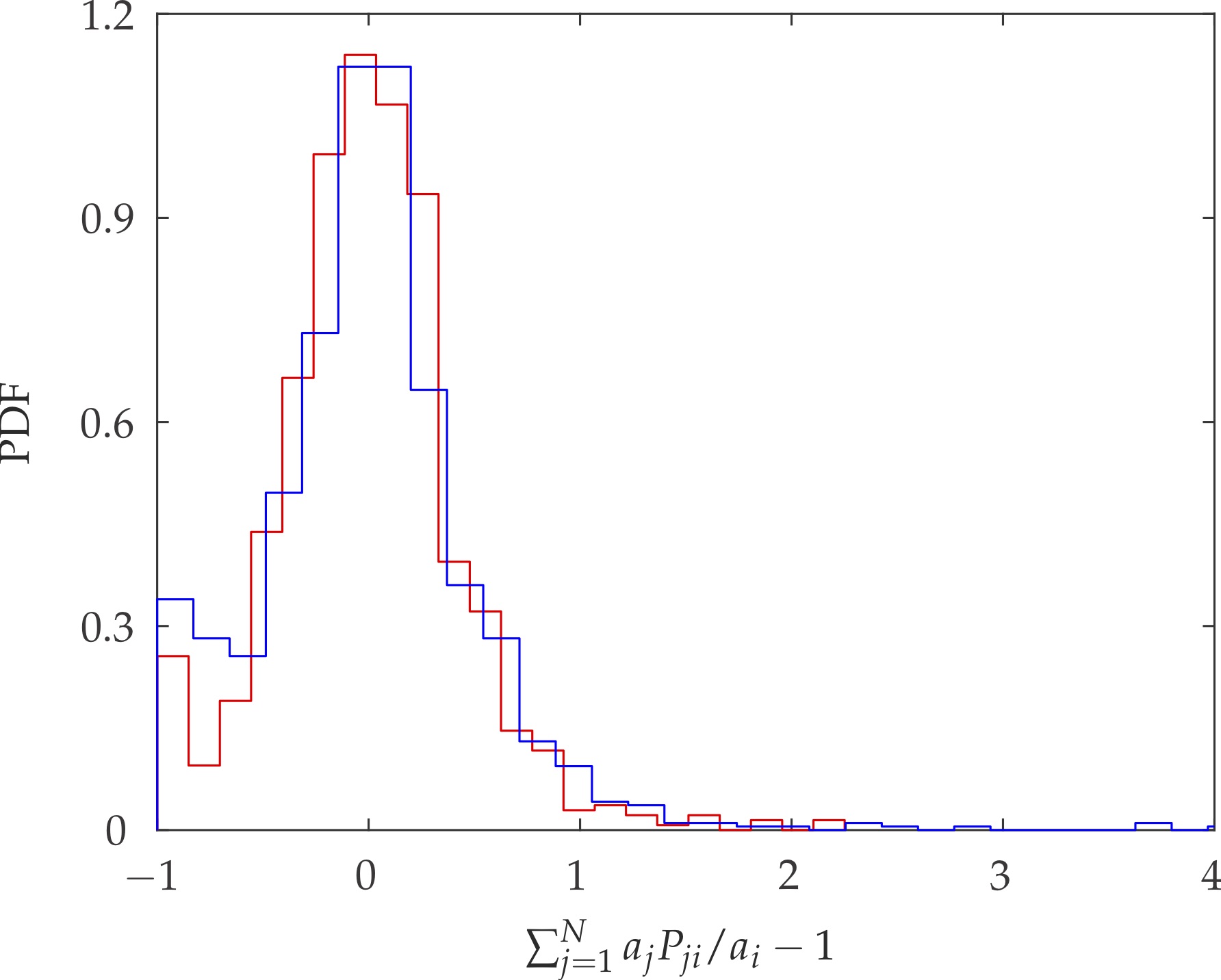
Figure 5: Probability density function estimates of relative area change computed over 7 days using the RAFOS deep float data (red) and satellite-track surface drifter data (blue).

4.4 Analysis of the Markov chain’s eigenspectrum

We now proceed to determine the level of connectivity within the horizontal domain in the layer visited by the deep floats by applying the eigenvector method on the matrix $P$.

The eigenspectrum of $P$ is composed of a total of $N=946$ eigenvalues.  As noted above, only eigenvectors of $P$ corresponding to eigenvalues close to unity are relevant, and because $P$ is very sparse, one may use Lanczos-type methods Lehoucq et al. (1998) to compute the $n\ll N$ largest eigenvalues.  With this in mind, we show in Fig. 6 the eigenspectrum of $P$ restricted to $\lambda>0.9$.  This top 10%  portion of the eigenspectrum includes 10 eigenvalues, yet not all 10 associated eigenvectors might need to be taken into account.  Indeed, thinking of $\lambda_{n}<1$ as a decay rate for a signed density revealed by the $n$th left eigenvector of $P$, if a large spectral gap between two collections of eigenvalues is present, then the densities revealed by the eigenvectors associated with eigenvalues prior to the gap will decay much more slowly and survive over much longer timescales than the densities revealed by the eigenvectors associated with the eigenvalues after the gap.  Therefore, the presence of a pronounced eigengap provides rationale for stopping eigenvector analysis. However, inspection of Fig. 6 does not reveal any gap that strongly suggests a cutoff for analysis except, perhaps, at $n=8$ or $n=6$.  Yet only the gap at $n=6$ may be considered significant with respect to the uncertainty of the eigenvalue computation.  The gray shade in Fig. 6 represents an uncertainty of the computation of $\lambda_{n}$ as measured by the median absolute deviation about $\lambda_{n}$ in an ensemble of 1000 realizations computed from transition matrices constructed using randomly perturbed float trajectories with 5 km amplitude, corresponding to the float positioning accuracy.  This uncertainty measure grows noticeably beyond $n=8$, making the gap there not significant.  This suggests, in the absence of evidence establishing any better criterion, that the analysis should not be extended beyond the 6th eigenvector.  It must be noted that we have so far implicitly referred to the real eigenspectrum of $P$.  Interspersed among the dominant eigenvalues (in absolute magnitude) are complex-conjugate eigenvalue pairs.  We will discuss a relevant complex eigenvector pair after discussing the real eigenvectors, restricted to the first 6 as just articulated.

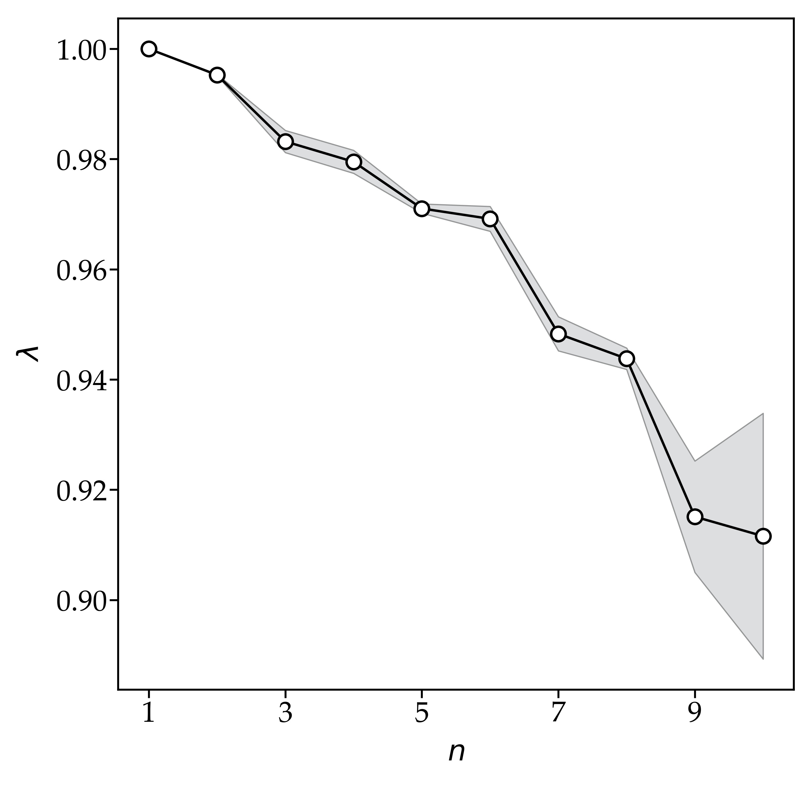
Figure 6: A portion of the discrete eigenspectrum of the transition    matrix $P$ showing the top 10 real eigenvalues (circles) and    uncertainties (gray shade) representing the median absolute    deviation about them in ensemble of eigenvalues computed using    transition matrices produced by randomly perturbing the float    trajectories.

As expected from the assessment of communication within the Markov chain associated with $P$, to numerical precision its largest eigenvalue, $\lambda_{1}=1$, is simple. The corresponding left and right eigenvectors are shown in the left and right panels of Fig. 7, respectively. The right eigenvector is flat as required by row-stochasticity of $P$, which is exactly satisfied given that no floats exit the domain $X$ on which $P$ is defined (the physical significance of this domain being closed is discussed below). The left eigenvector is positive within the absorbing closed communicating class of states of the Markov chain, which covers most of the boxes of the partition (cf. Fig. 3), and vanishes elsewhere. Furthermore, the structure of the left eigenvector resembles quite closely the distribution of the probability density in the rightmost panel of Fig. 4. More precisely, this is nearly equal to the left eigenvector when normalized by the area of the boxes in the partition, confirming its invariant, limiting nature.

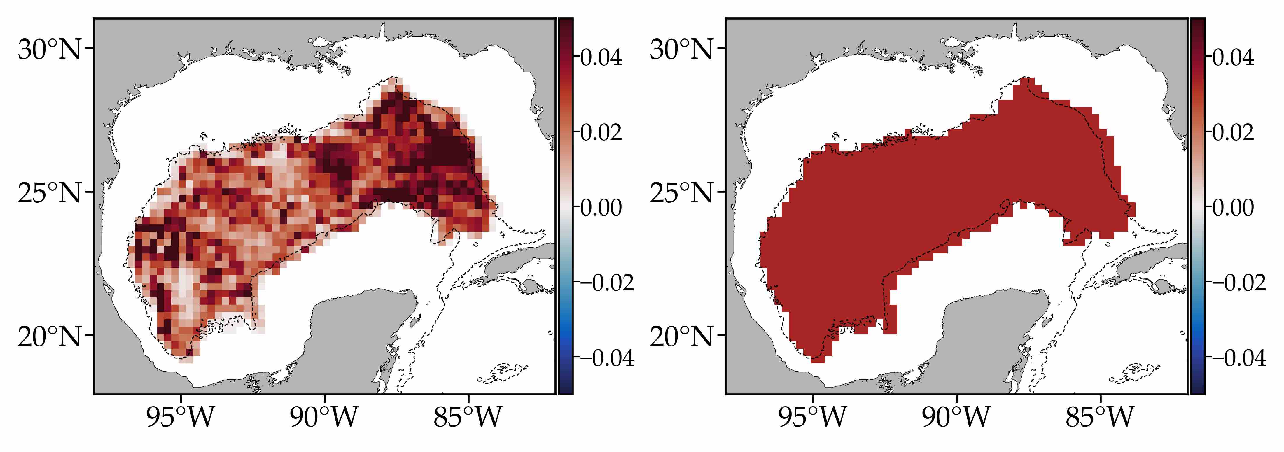
Figure 7: Left (left panel) and right (right panel) eigenvectors associated with the largest eigenvalue of $P$, $\lambda_{1}=1$. The left eigenvector is invariant: $pP=p$. The right eigenvector, a vector of ones by row-stochasticity of $P$, is mapped after infinitely many applications of $P$ to the left eigenvector ($\lim_{k\to\infty}(\mathbf{1}/N)P^{k}=p$), thereby representing a single basin of attraction for the invariant attractor revealed by the left eigenvector.

The top left and right panels of Fig. 8 respectively show the left and right eigenvectors associated with the 2nd largest eigenvalue of $P$, $\lambda_{2}=0.9943$. Note that the left eigenvector takes a single sign within each side of a zero-level curve that partitions the floats’ domain into two regions. Two basins of attraction are identified by the right eigenvector. These are given by the regions where the right eigenvector is approximately flat, i.e., approximately looks like $\mathbf{1}$. Splitting the domain into two regions between which there is weak interaction, the western (eastern) region constitutes a basin of attraction for the attractors revealed by the left eigenvector in the western (eastern) side of the domain. To make the connection between forward-time attractors and backward-time basins of attraction explicit, the eigenvectors have been assigned (in this and the subsequent figure) signs such that positive (negative) portions of the right eigenvector map to positive (negative) portions of the left eigenvector under repeated right multiplication by $P$. These attractors are not invariant, but rather will retain tracer for a finite period of time (intramixing timescales, loosely referred to as invariance timescales in Miron et al. (2017), can be estimated by thinking of $\lambda<1$ as a decay rate as noted above; more insightful measures of the invariance time of a set are provided by the residence and retention times in the set, which are considered below).

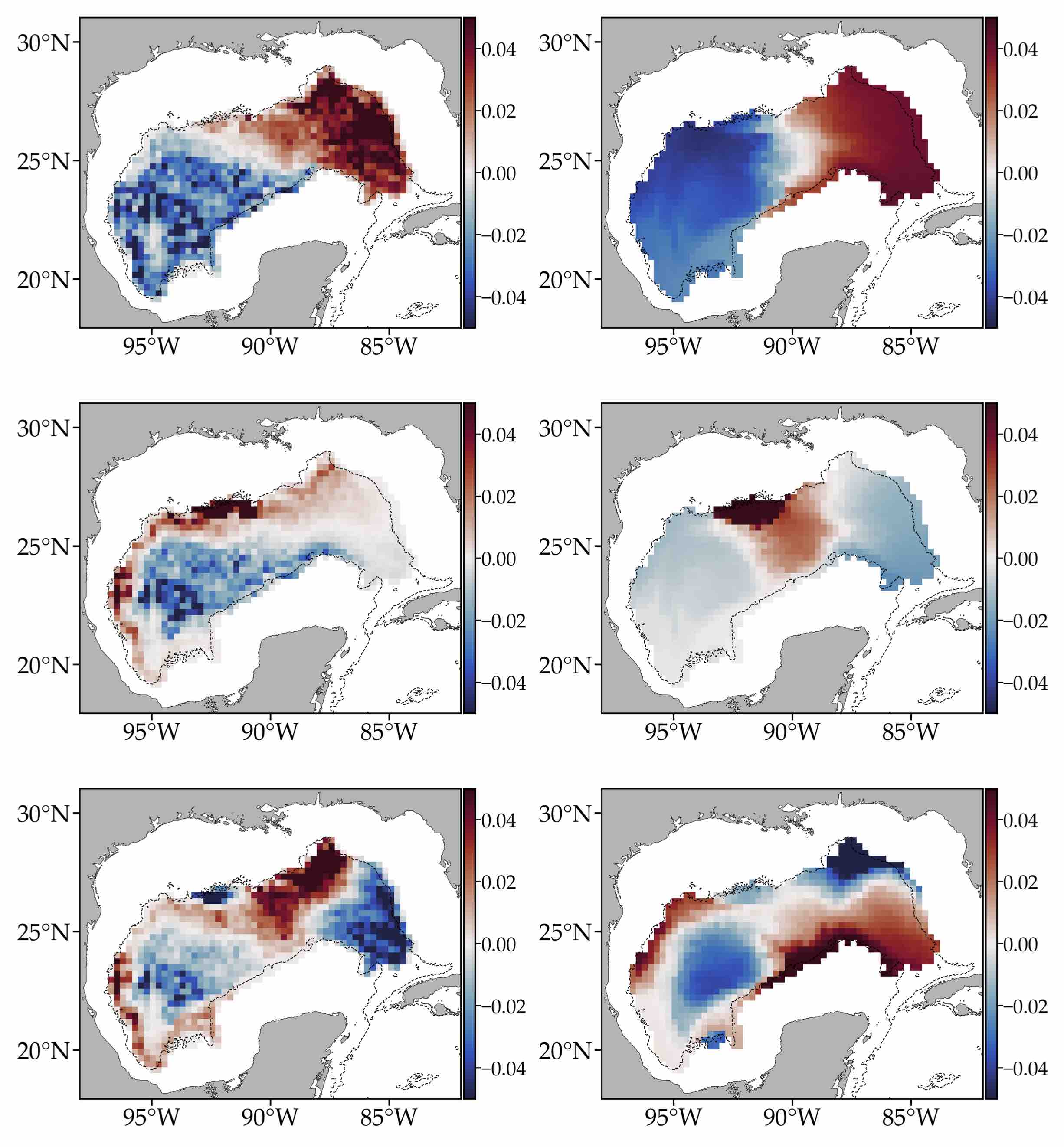
Figure 8: As in Fig. 7, but for $\lambda_{2}=0.9943$ (top), $\lambda_{3}=0.9822$ (middle), and $\lambda_{5}=0.9701$ (bottom). The left eigenvector reveals the locations of almost-invariant sets of forward-time attraction. The corresponding backward-time basins of attraction are revealed by the right eigenvector. The sign assignment is such that positive (negative) right eigenvector portions map to positive (negative) left eigenvector portions under repeated left multiplication by $P$.

Inspection of the left eigenvector associated with the 3rd largest eigenvalue of $P$, $\lambda_{3}=0.9822$, reveals further attracting sets, but with shorter invariance timescale (Fig. 8, middle-left panel). One such set in particular, highlights a tendency of the Lagrangian motion to circulate along the 1500-m isobath on the western side of the domain for tracers initially covering a large sector in the center of the domain. The latter is revealed in the right eigenvector (Fig. 8, middle-right panel), which is nearly flat in the noted central sector. The right eigenvector is also approximately flat on two regions flanking this sector which are weakly connected through a very narrow channel running along the southern edge of the domain. The two regions cover the entire domain, forming two basins of attraction for almost-invariant sets in the regions of the left eigenvector with like sign.

Additional almost-invariant attracting sets (with shorter invariance timescales) and corresponding basins of attraction are revealed by the left–right eigenvector pairs associated with the 4th to 6th eigenvalues of $P$ (cf., e.g., the 5th pair in the bottom row of Fig. 8). Patching together these and the above basins of attraction the various Lagrangian geographic partitions shown in Fig. 9 are obtained.

4.5 Lagrangian geography

Rather than thresholding right eigenvectors as in prior applications (Froyland et al. 2014; Miron et al. 2017), the various provinces in each Lagrangian geography constructed here were automatically obtained by applying a $k$-means clustering algorithm (Kaufman and Rousseeuw 1990) that minimizes squared Euclidean distance as outlined in Algorithm 1 of Froyland (2005), but with the weighted fuzzy clustering replaced with $k$-means clustering. The main geographic partition in the left panel of Fig. 9 was obtained by seeking $k=2$ clusters in the 2nd right eigenvector of $P$.  Refined geographic partitions, shown in the middle and right panels, resulted by considering more eigenvectors in the relevant set suggested by the eigenvalue uncertainty computation and eigengap inspection. The refined partition in the right panel of Fig. 9 was obtained by seeking $k=6$ clusters in the 2nd through 6th right eigenvector. The middle panel shows an intermediate partition resulting from seeking $k=4$ clusters in the 2nd through 4th right eigenvector. Seeking $k=2$ clusters from the 2nd eigenvector is an obvious choice that follows from direct inspection of this eigenvector. Seeking $k=K>2$ clusters from the 2nd through $K$th eigenvectors assumes that each right eigenvector adds a new province to the geography at a time. The silhouette value $-1\leq s\leq 1$ (Rousseeuw 1987) is a measure of how similar an object is to its own cluster compared to other clusters, with a large $s$ indicating that the object is well matched to its own cluster and poorly matched to neighboring clusters. The mean $s$ equals to 0.91, 0.54 and 0.56 for the clusters identified using $k=2$, 4, and 6 when the first 2, 4, and 6 right eigenvectors are taken into account, respectively. Larger $k$ in the latter two cases can produce more consistent clusters, albeit much smaller and hence with shorter residence or retention times, so we have not considered them.

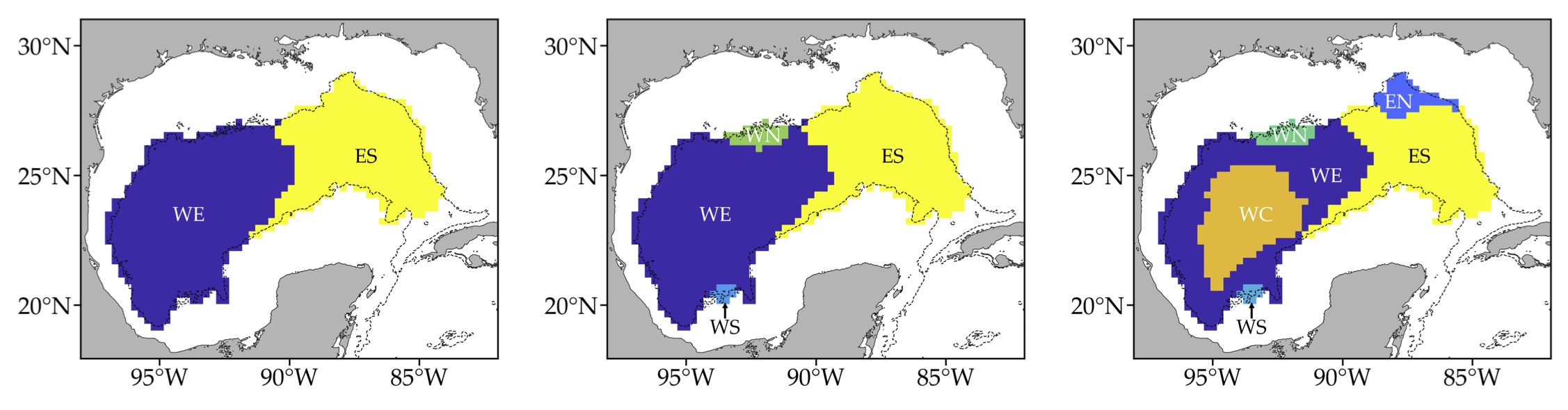
Figure 9: Lagrangian geography of dynamically weakly interacting provinces formed by the domains of attraction associated with the most persistent attractors. Geographic partitions based on the analyses of the 2nd right eigenvector, 2nd through 4th right eigenvectors, and 2nd through 6th right eigenvectors are shown in the left, middle, and right panels, respectively.

In the 2-eigenvector geography 2 large provinces, one western (WE) and another one eastern (ES), split the domain nearly in half. The 4-eigenvector geography incorporates two provinces in WE: a small northern subprovince (WN) and another southern subprovince (WS) even smaller. The 6-eigenvector geography incorporates to WE these same small subprovinces and another, much larger, central subprovince (WC). Province ES is not modified by the 4-eigenvector geography, while the 6-eigenvector geography alters it by the addition of a small northern subprovince (EN).

As constructed, the provinces of the above Lagrangian geographies only weakly dynamically interact. This imposes constraints on connectivity within the 1500-to-2500-m layer in the GoM. More specifically, the communication between any two provinces is constrained locally by the level of invariance of the attractors contained within each of them and remotely by that of any attractors outside of the provinces but sufficiently close to them.

The level of communication among provinces can be assessed by the computation of forward-time conditional transition probabilities between pair of provinces. Over 7 days, the mean inter-province probability percentages are 98.5, 97.5, and 94.3 for the 2-, 4-, and 6-eigenvector geographic partitions. Note that these are high, indicating weak intra-province dynamical interaction. Note also that the percentages decrease as the number of provinces in the geography increases. This reflects in part that communication within large provinces is less constrained than across their boundaries. The resulting transition matrices restricted to the various geographies are not symmetric, revealing the asymmetric nature of the Lagrangian dynamics in time. The asymmetry grows with the number of provinces in the partition, as can be expected.

From left to right, Figure 10 shows residence time estimates according to formula (8) within each of the provinces in the 2- to 6-eigenvector Lagrangian geographies. Note that $\tau$ decreases outward down to $\tau=0$ at the boundaries of the provinces. As expected, the maximum values tend to be attained where the right eigenvectors of $P$ locally maximize (in absolute magnitude). These regions, as described above, correspond to basins that are attracted toward forward time almost-invariant attracting sets. The small values of $\tau$ attained in the periphery of the provinces (basins of attraction corresponding to those attractors) simply indicate that mixing with neighboring provinces begins at their boundaries.

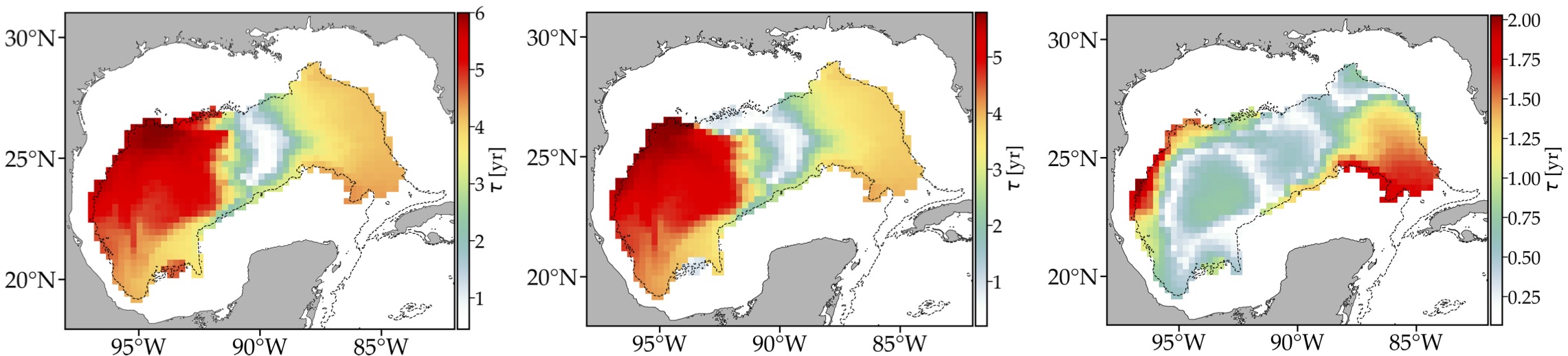
Figure 10: Estimates of residence time within provinces in the 2- (left), 4- (middle), and 6-eigenvectors (right) Lagrangian geographies. Note the scale range differences.

The residence time calculation shows a west–east asymmetry in the 2-eigenvector geography, with the WE province having longer residence times than the ES province. Specifically, the mean residence time in WE (ES) province is of about 4.53 (3.38) years. It must be mentioned that the mean here is taken with respect to a uniform probability distribution, i.e., it is computed as an average according to Lebesgue (area) measure. As noted earlier in the paper, mean residence times computed using (8) coincide with retention times (10) based on the likelihood of a trajectory to survive in a given set if the mean in the former is taken according to the probability distribution given by the leading left eigenvector of $P$ restricted to the set in question. The resulting mean residence (or, equivalently, retention) times are 4.74 and 3.74 years for the WE and ES provinces, respectively, which are very similar to the values stated above.

The provinces in the 4- and 6-eigenvector geographies have shorter residence times. For instance, on average within the WE, WS, WC, WW, ES, and EN provinces in the 6-eigenvector partition these are about 0.74, 0.90, 0.48, 0.64, 1.18, and 0.38 years, respectively. Shorter residence times in sets covering smaller areas are expected. But note the short residence time of the WC province despite its large coverage.

The direct pushforward of tracers with $P$ further revealed that the slow exchange between the main provinces is executed from east (west) to west (east) through a northern (southern) corridor. This suggests a slow cyclonic circulation in the deep GoM. Such a preferred circulatory motion is consistent with the peculiar shape of the geography in the western side of the domain, which includes an enclave around which tracers will tend to circulate before exchange of material is effected. This explains the residence time asymmetry of the main provinces.

The west–east residence time asymmetry can be further realized by computing the time it takes on average to hit or reach a given province starting in another province. This can be done using (8) with the region $A$ set to the complement of the target province. The result of this calculation for the 6-eigenvector geographic partition is shown in Table 1. The top row shows source provinces and the left column target provinces. Consider for example the bottom row. The mean time to hit EN in the eastern basin starting on WC in the western side of the domain is 6.17 years. Consider now the second-to-top row. To reach WC from EN it takes on average 1.91 years. Consistent with west–east residence time asymmetry, it takes more than three times as long to reach EN from WC. Clearly, the mean time to reach a given province starting in the same province is 0. Note that WS has not been included in the table as this province is never reached from outside.

Table 1: Mean time (in years) to reach a province of the 6-eigenvector Lagrangian geography indicated in the left column starting from any province in the top row.

	WE	WC	WW	ES	EN
WE	0.00	0.26	0.41	0.68	0.86
WC	1.05	0.00	1.46	1.73	1.91
WW	7.97	8.23	0.00	8.64	8.82
ES	1.51	1.76	1.90	0.00	0.20
EN	6.17	6.42	6.56	4.68	0.00

5 Validation

5.1 Chemical tracer

The deep Lagrangian geography constructed here and the surface Lagrangian geography computed by Miron et al. (2017) are globally different on the overlapping domains, suggesting that the surface Lagrangian motion is to a large extent decoupled from the deep Lagrangian motion. An important exception is the partition by a roughly meridional boundary of the surface and deep domains into two basins of attraction for almost-invariant attractors revealed by the inspection of eigenvectors of the corresponding transition matrices with the 2nd-largest nonunity eigenvalue (compare the left panel of Fig. 9 and the left panel of Fig. 6 of Miron et al. (2017)).

The restricted connection at depth between the eastern and western GoM was suggested by the behavior of profiling floats parked at about 900 m launched in the eastern side, which tended to stay there, and those launched in the western side, which remained there for a long period of time (Weatherly et al. 2005). Here we provide support for the significance of the partition of the deep GoM domain at a deeper level using the observed evolution of the chemical tracer injected near the Deepwater Horizon oil rig during the field experiment described by Ledwell et al. (2016).

The right panels of Fig. 11 show the distribution taken by the chemical tracer 4 (top) and 12 (bottom) months after release. The release site lies about 100-km southwest of the cross, indicating the location of the Deepwater Horizon rig. The circles are colored according to the amount of tracer found during in-situ casts, integrated vertically between 1000 and 2500 m. The colored background is a smoothed interpolated map based on the station data. Note the tendency of the tracer to spread over the eastern side of the domain. After 12 months from release, little tracer is seen to have traversed the zero-level set of the left eigenvector of $P$ with the largest eigenvalue (indicated by a solid line). And note that absolutely no tracer at all was detected during the in-situ casts made well in the western side of the domain. This is consistent with the expected fate of a tracer probability density initiated on the main eastern province of the Lagrangian geography constructed from the float data.

This expectation is confirmed by the evolution of a tracer probability started from a source location near the chemical tracer release site under the action of the transition matrix $P$ (Fig. 11, left panels). Consistent with the chemical tracer evolution, the (synthetic) tracer probability spreads similarly over the eastern side of the domain without significantly crossing the zero-level set of the largest nontrivial eigenvector.

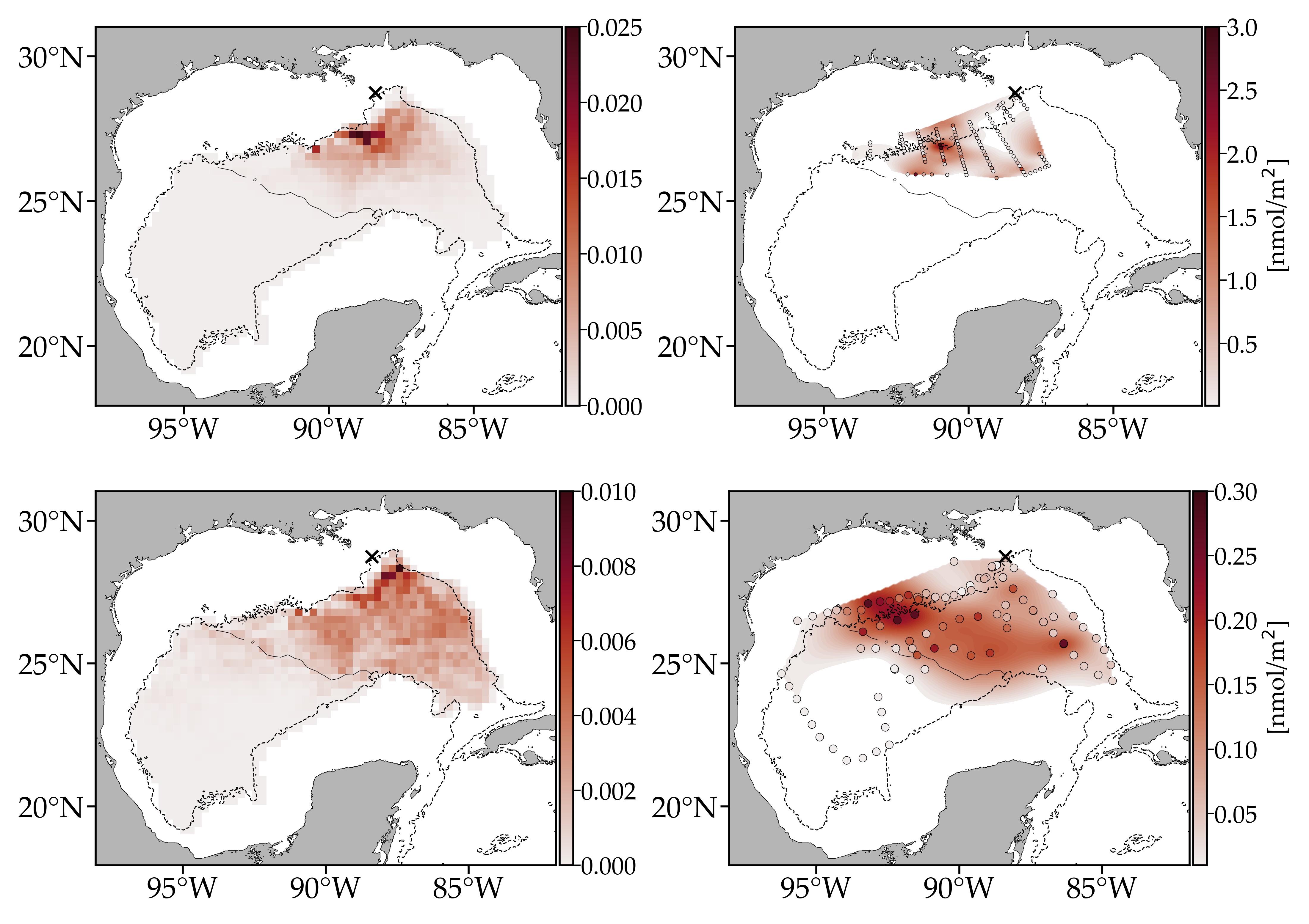
Figure 11: Comparison between the evolution of a tracer probability density under the action of the transition matrix $P$ (left column) and dispersion of a chemical tracer (right column) presented both after 4 (top row) and 12 (bottom row) months of released about 100-km southwest of the Deepwater Horizon site (indicated by a cross). On the right column, the colored background is an interpolated map based on column integral of tracer found during in-situ casts at the station locations (colored circles). The solid line in each panel indicates the zero-level set of the left eigenvector of $P$ associated with the 2nd largest eigenvalue.

It must be noted, however, that as the tracer probability is continually being pushed forward under $P$, it will eventually spread over the western basin along its northern boundary of the domain, describing a cyclonic circulatory pattern as noted above consistent with inferences made from the direct inspection of float trajectories, the analysis of hydrography and mooring data, and numerical simulations (Hurlburt and Thompson 1980; Oey and Lee 2002; Mizuta and Hogg 2004; DeHaan and Sturges 2005; Bracco-etal-06; Hamilton et al. 2016; Pérez-Brunius et al. 2017; Tenreiro et al. 2018). Also consistent with direct inspection of trajectories (Hamilton et al. 2016; Pérez-Brunius et al. 2017), and high resolution modelled fields (Bracco-etal-06), some probability tracer will circulate cyclonically around the enclave inside the main western province of the Lagrangian geography.

5.2 Profiling floats

Additional independent observational support for the significance of the results obtained from the analysis of the Markov-chain model derived using the RAFOS floats is provided by the analysis of a Markov-chain model constructed using Argo profiling floats drifting at an average parking depth of $1000$ m. At a shallower depth, the Argo trajectories sample a similar horizontal domain of the GoM as the RAFOS trajectories, but less densely (there are only 60 Argo floats in the database analyzed). Also, the temporal coverage of the Argo floats is not as ample as the RAFOS floats. With these differences in mind we constructed a matrix of probabilities of the Argo floats to transitioning between the boxes of a grid similar to that used with the RAFOS floats. The transition time was set to 7 days as in RAFOS floats analysis, which required us to interpolate the original 10-daily trajectories. The Markov chain associated with the resulting $P$ was found to be characterized by an absorbing closed communicating class of states spanning most boxes of the partition. Thus $\lambda_{1}=1$ was found to be the only eigenvalue of $P$ on the unit circle, implying the existence of a limiting invariant probability vector. The structure of the left–right eigenvector pair for the 2nd eigenvalue is shown in Fig. 12. Albeit more noisy and gappy, this pair shows similarities with that of the $P$ computed using the RAFOS floats (Fig. 7, top row). Indeed, a partition of the domain nearly into 2 basins of attraction is evident. This adds confidence to the RAFOS float analysis. It also suggests a tendency of the motion to be preferentially columnar in the deep GoM (recall that the Argo floats ascend to transmit positions at the surface while the RAFOS floats remain parked at a fixed level at all times during an experiment).

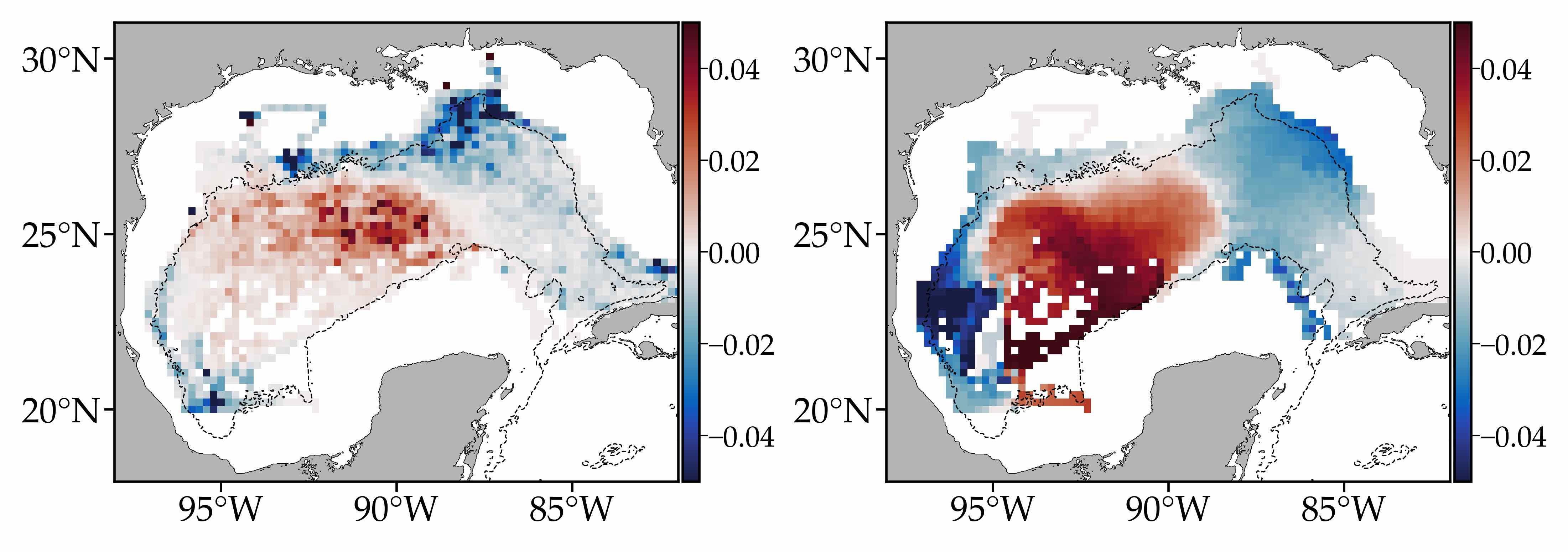
Figure 12: As in the top row of Fig. 8, but based on Argo profiling floats.

6 Discussion

6.1 Cyclonic circulation and f/H

The cyclonic circulation in the western side of the GoM domain is well described by complex eigenvectors of $P$. Let $v_{\pm}$ be a complex-conjugate left eigenvector pair of $P$ with $\lambda_{\pm}=r\smash{\operatorname{e}^{\pm\operatorname{i}\theta}}$, where $\theta\geq 0$. After $k$ applications of $P$, $v_{\pm}P^{k}=r^{k}v_{\pm}\smash{\operatorname{e}^{\pm\operatorname{i}k\theta}}$. Viewing each complex component of $v_{\pm}$ as a vector in $\mathbb{C}$, if $r\approx 1$ the latter represents a rotation of each such vectors by an angle $\pm k\theta$. Furthermore, $v_{\pm}P^{k}$ returns to $v_{\pm}$ after $k_{*}=2\pi/\theta$ applications of $P$. Because $k_{*}$ need not be an integer, $v_{\pm}P^{k_{*}}$ will not in general exactly coincide with $v_{\pm}$, which represents almost-cyclic sets. Figure 13 shows $\operatorname{Re}\!{(v_{\pm}P^{k})}$ where $v_{\pm}$ corresponds to the leading $\lambda_{\pm}$ (for which $r=0.9775$ and $\theta=0.0239$) for several $k$ over an almost cycle (with period $k_{*}T=5.0414$ years). Independent of whether $v_{+}$ or $v_{-}$ is considered, note the cyclonic rotation described in the western main province of the Lagrangian geography.

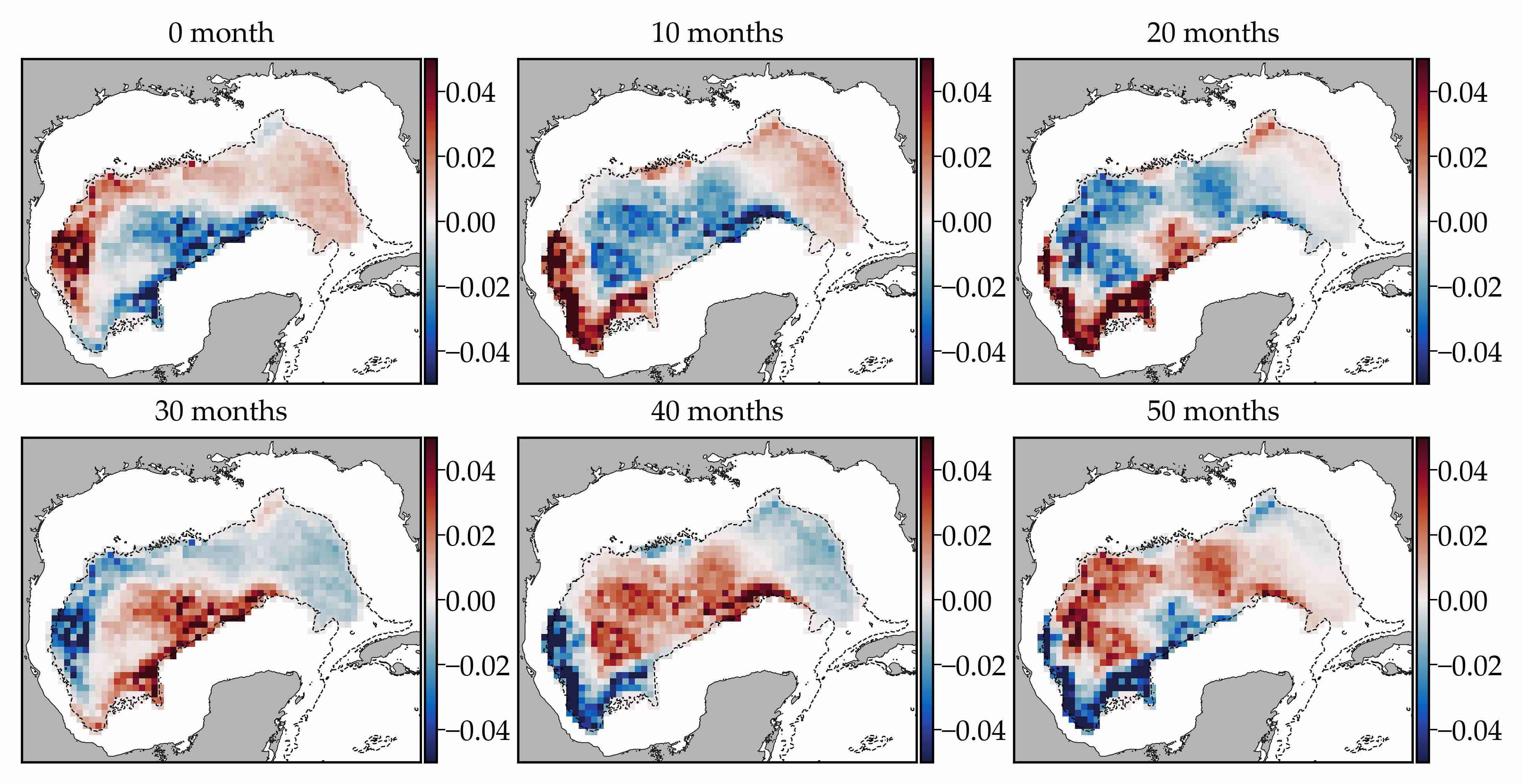
Figure 13: Snapshots of the forward evolution of the leading complex left eigenvector of transition matrix $P$ over an almost cycle (with a period of 60.5 months). The real part is shown. The result does not depend on the member of the complex-conjugate eigenvector pair considered.

Rectification of topographic Rossby waves has been identified as a driver for the cyclonic circulation along the boundary (Hurlburt and Thompson 1980; Oey and Lee 2002; Mizuta and Hogg 2004; DeHaan and Sturges 2005). In linear, unforced, inviscid, barotropic and quasigeostrophic dynamics (Gill 1982), the vorticity changes only when there is motion across the $f/H$ contours, where $f$ is the Coriolis parameter (twice the local vertical component of the Earth’s angular velocity) and $H$ is the fluid depth. As such, $f/H$ provides a restoring force, supporting topographic Rossby waves, which through nonlinear interaction can be rectified to give rise to a mean flow directed mainly along $f/H$ isolines (Colin de Verdiere 1979). Here we test $f/H$ conservation using the Markov-chain model and further assess its effect on the evolution of probability tracer densities in the domain.

Specifically, let $Q_{j}=f_{j}/H_{i}$ be the mean value of $f/H$ inside box $B_{j}$ in the partition. To first-order approximation, $Q_{j}$ must be preserved along tracer trajectories entering box $B_{j}$. To check this, we propagate backward the observable $f/H$ by $k$ steps with the transition matrix $P$. Define $q_{i}:=\smash{\sum_{j=1}^{N}P_{ij}^{k}Q_{j}}$, the $i$th component of the backward propagation of $Q$, averaged over those boxes $B_{j}$ that the forward propagation of $B_{i}$ intersects. If $f/H$ were exactly preserved along trajectories, then one would expect $q_{i}=Q_{i}$.

Figure 14 shows $\varepsilon_{i}:=|q_{i}/Q_{i}-1|$ after $k=52$ applications of $P$ (corresponding to 1-year forward evolution). Note that $f/H$ is preserved with 25%  error or less along the western and southern boundaries of the domain and over a large region of the eastern side of the domain. Because the restoring force provided by $f/H$ is largest where $f/H$ varies rapidly, tracer trajectories initially on the western boundary will be constrained to run along that boundary as the gradient of $f/H$ across isobaths there is large ($f$ is relatively constant in the domain). A similar behavior may be expected for trajectories starting on the southern boundary across which $f/H$ changes rapidly. However, $f/H$ is not uniformly preserved along this boundary. Indeed, boxes where $\varepsilon_{i}$ are interspersed among boxes where this is small. As a consequence, trajectories starting on that boundary are not expected to be so constrained to run along. In the eastern portion of the domain where $\varepsilon_{i}$ is small, the bottom is relatively flat. As a result, trajectories starting will unlikely follow any particular $H$ isoline while nearly conserving $f/H$. Moreover, this will tend to occupy the domain in question, which resembles quite well the positive side of 2nd left eigenvector of $P$ (cf. Fig. 8, upper panel). Finally, in the large western region where $\varepsilon_{i}$ is large, the trajectories will wander unrestrained within the region, which itself resembles quite well the negative side of 2nd left eigenvector of $P$.

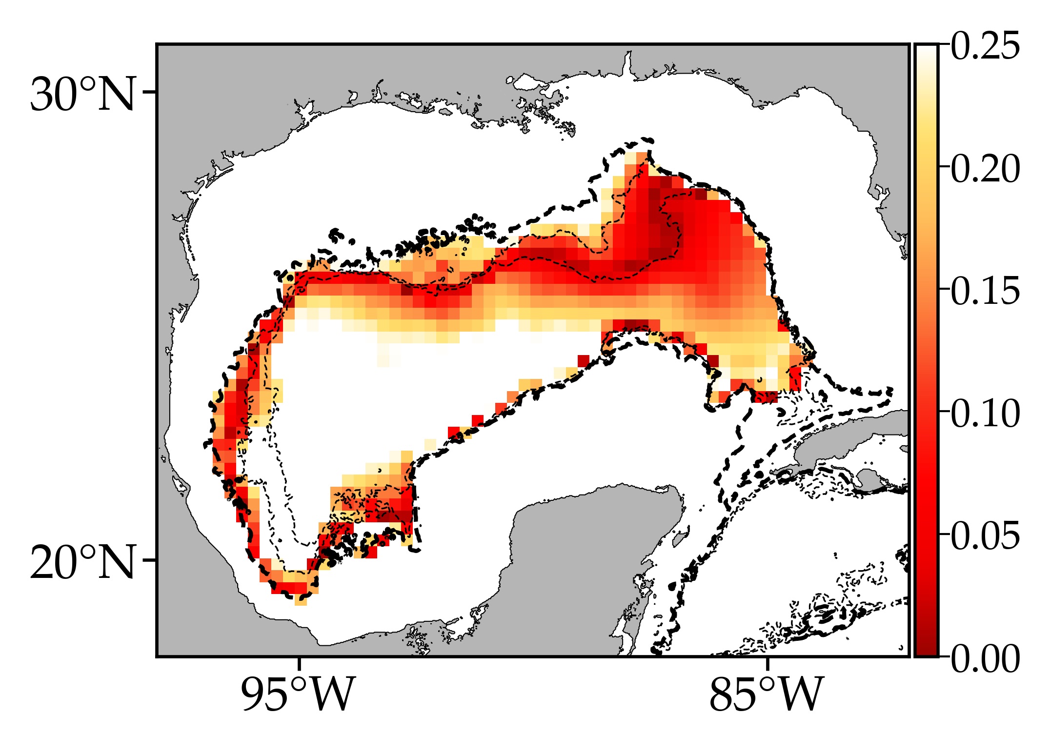
Figure 14: For each box in the partition, absolute relative error between $f/H$, where $f$ is the Coriolis parameter and $H$ is depth, and the average of $f/H$ according to the forward evolution over 1 year of a probability vector supported in the box. Dashed lines are the isobaths of 1750, 2500, 3000 m.

The expected behavior of tracer trajectories deduced from the Markov-chain model is verified by the behavior observed float trajectory patterns. This is shown in Fig. 15 for groups of float trajectories that have gone through selected sites along the boundary of the domain (left) and the center of the western side of the domain (right). Note, in the left panel, how the red and orange trajectories tend to run along the western boundary, while the green trajectories are not so constrained to doing so along the southern boundary. Observe too in this panel how the blue trajectories cover the eastern side of the domain consistent with $f/H$ being preserved in that region. Finally, note that the trajectories in the right panel loop around in a largely unrestricted manner.

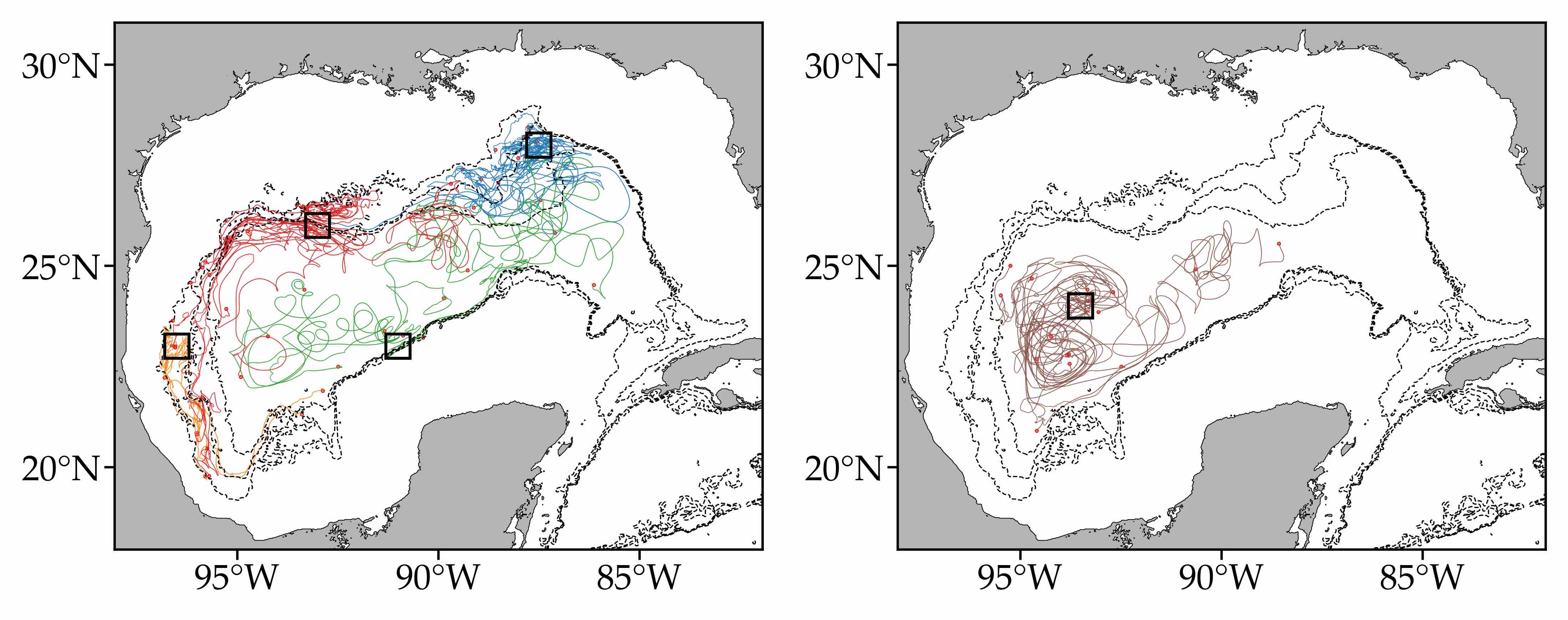
Figure 15: Trajectories of floats that, having gone through the boxes indicated, are constrained by $f/H$ conservation on different levels (left) and are not constrained by $f/H$ preservation.

6.2 Homogeneization

The analysis of the chemical tracer injected at depth suggested that homogenization in the GoM is more rapid than in the open ocean (Ledwell et al. 2016). While the Markov-chain model constructed here does not predict uniform homogenization in the long run, it supports a limiting, invariant distribution which does not reveal a preferred region for accumulation but rather a multitude of different small regions where some accumulation is possible. The highly structured texture of this distribution suggests partial homogenization in the long run. This can be quite fast. For instance, for a tracer released in the eastern side of the domain, it can take as short as 1 year or so to spread over that portion of the domain (cf. Fig. 10) consistent with the good agreement between the forward evolution of a tracer probability and the observed chemical tracer spreading (recall Fig. 11). This corresponds well with the mean time required for the EN province to hit the WE province, which is of 0.86 years (cf. Table 1 and Fig. 9).

6.3 Ventilation

Below 1000 m the GoM is filled with oxygen-rich water which is isolated from diffusive inflow of oxygen from the surface by the presence of a layer of oxygen-poor water (Nowlin et al. 2001). As standard deep-water formation is very unlikely due to the extreme cooling and salinity increase required for the surface layer to sink, ventilation of the deep GoM has been argued to be accomplished via horizontal transport of oxygen-rich water from the Caribbean Sea (Rivas et al. 2005).

The tendency of the Lagrangian motion as inferred from the Markov-chain model constructed using the RAFOS floats to conserve area more effectively than that using surface drifters, together with the similarities of the dominant eigenvectors of the transition matrices built using RAFOS and Argo floats, is consistent with the above observations in that Lagrangian motion within the 1500–2500-m layer is predominantly horizontal. However, the Markov-chain model does not represent exchanges through the boundary of the domain on which is supported as the RAFOS floats deployed inside the domain do not escape the domain.

Yet the above does not rule out the possibility that floats deployed outside the domain eventually enter the domain. Indirectly, this possibility is described by our Markov-chain model. This is shown in Fig. 16 for a tracer probability density initially at the southeastern corner of the domain. Note that it spreads over the domain, mainly cyclonically and along the eastern boundary, under the action of $P$ as opposed to accumulate in the southeastern corner. This suggests a horizontal ventilation pathway from the Caribbean Sea compensated by weak vertical mixing.

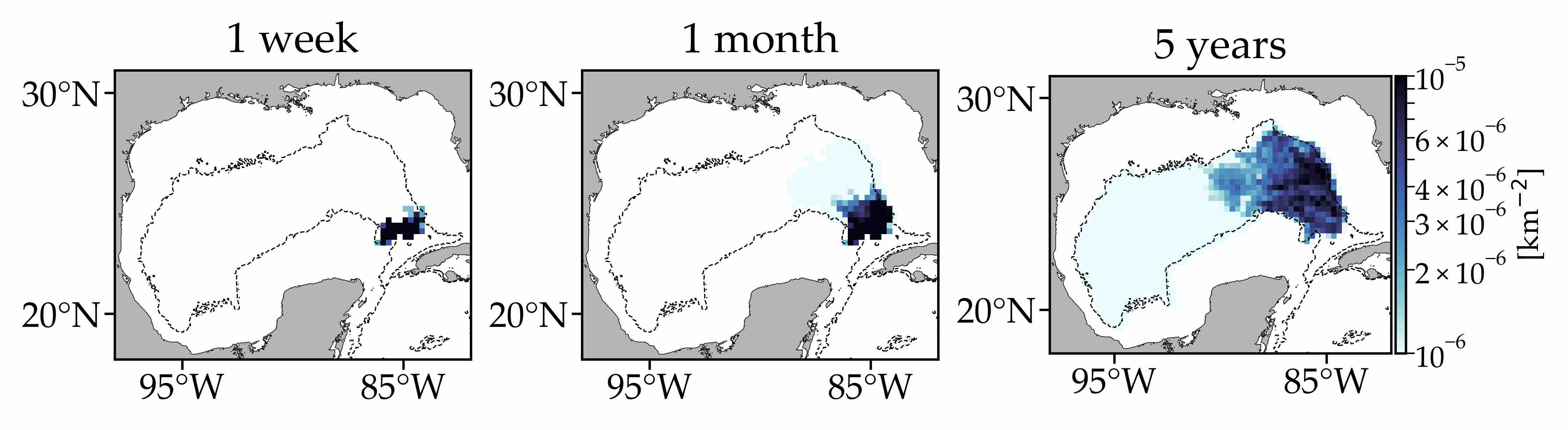
Figure 16: Snapshots of the evolution under the action of the RAFOS-float-based transition matrix of a tracer probability density initially in the southeastern corner of the domain.

It must be noted that there are no RAFOS floats that can be used to verify the existence of that pathway. However, the Argo floats might suggest it at about 1000 m. This is shown in Fig. 17 for a few Argo float trajectories that start in the Caribbean Sea. We say “might” because we do not know for certain that the Argo floats penetrate the GoM domain at their parking depth or at shallower level in their ascend and descend. Ventilation might well be taken place more effectively at a shallower level as suggested by the observation that the core of the North Atlantic Deep Water (NADW), which fills the Caribbean Sea at depth, located between 1200 and 1300 m (Hamilton et al. ).

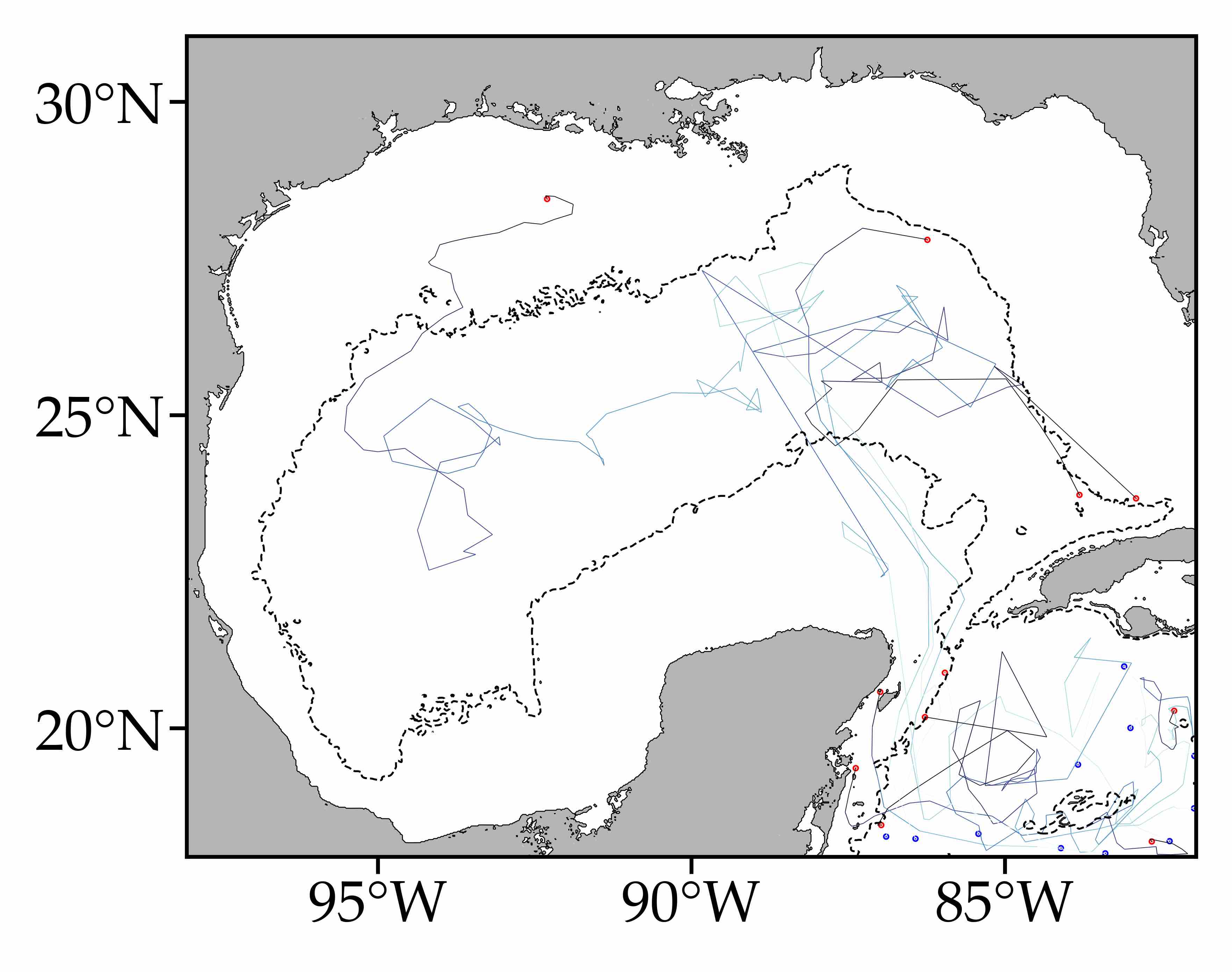
Figure 17: Trajectories of Argo profiling floats starting inside the Caribbean Sea. Initial positions are indicated by a blue dot and final positions by a red dot.

6.4 Mean circulation

We close the discussion by showing that the results obtained using the Markov-chain model could not have been revealed by simply inspecting the mean circulation deduced from the RAFOS float trajectories. The top panel of Fig. 18 shows ensemble-mean streamlines computed by integrating a steady velocity field resulting from averaging the float velocities in each box of the grid used to construct the Markov-chain model. While the streamlines suggest a cyclonic flow along the periphery of the domain especially on its western side, which is consistent with the transfer operator analysis and also direct inspection of float trajectories (Hamilton et al. 2016), it is difficult to find a correspondence among the many sources and sinks with the various local minima and maxima of the limiting, invariant distribution of the Markov-chain model (cf. the rightmost panel of Fig. 4 or the left panel of Fig. 7). The differences with the Markov-chain model results are most clearly evidenced when the evolution of a tracer under the corresponding flow is compared with the push forward of a tracer probability density under the transition matrix $P$. Snapshots of the evolution of a narrow Gaussian about near the chemical tracer injection site are shown after 4 and 12 months in the bottom-left and right panels of Fig. 18, respectively. Note that the spread of the tracer is confined to the vicinity of this site, which is in stark contrast with the much wider spreading of a probability density source initially near the same location under action of $P$ or the evolution of the chemical tracer injected nearby (cf. Fig. 11).

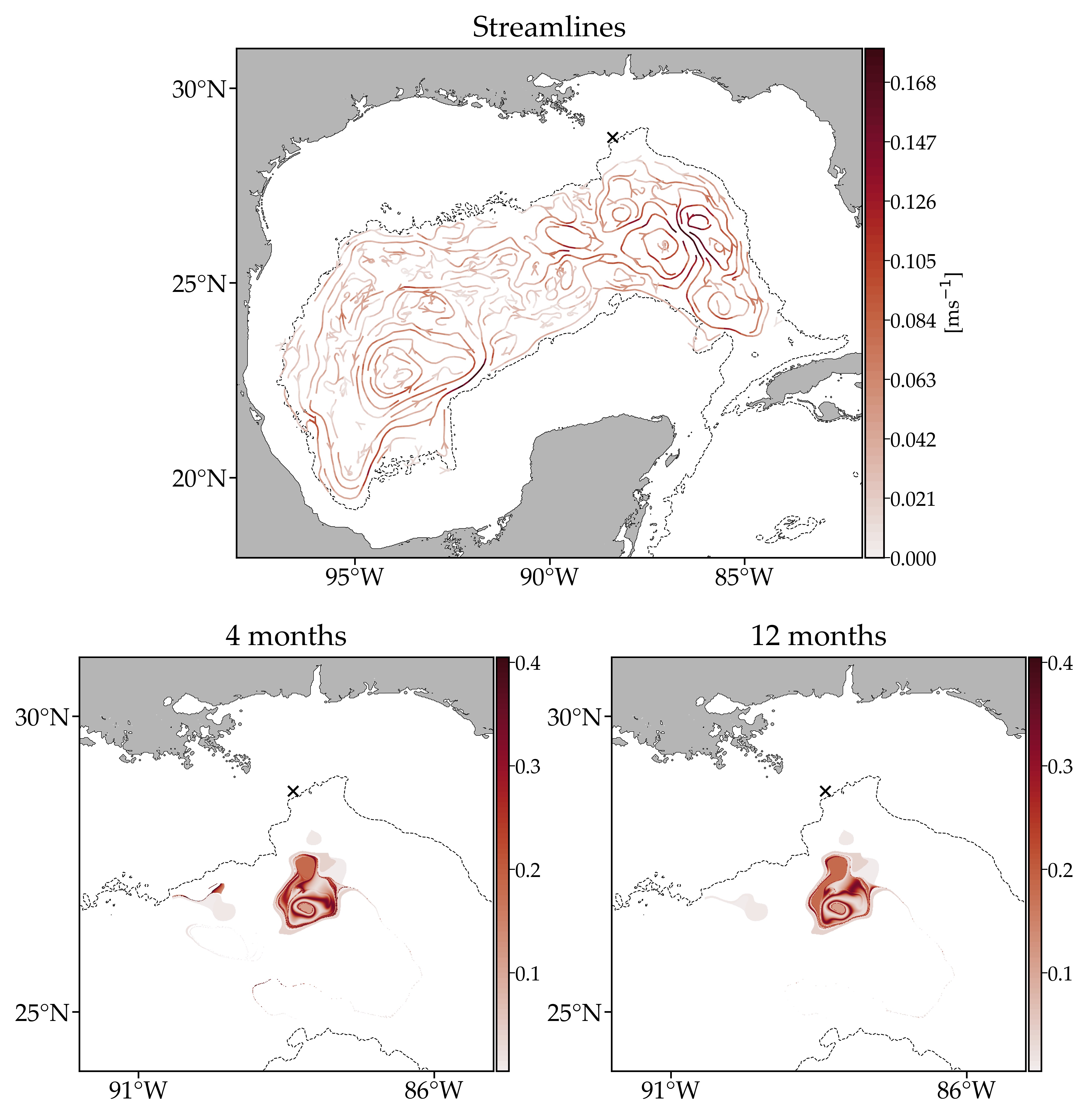
Figure 18: Ensemble mean streamlines computed using RAFOS float velocities (top) and snapshots at 4 (bottom-left) and 12 (bottom-right) months of the evolution under the corresponding flow of a narrow Gaussian initially centered about 100-km southwest of the Deepwater Horizon oil rig, indicated by a cross.

7 Summary and concluding remarks

Analyzing acoustically tracked (RAFOS) float data in the Gulf of Mexico (GoM), we have constructed a geography of its Lagrangian circulation within the deep layer between 1500 and 2500 m revealing aspects of the circulation transparent to standard Lagrangian data examination as well as confirming, and thus providing firm support to, other aspects already noted from direct inspection of the float trajectories. The analysis was done by applying a probabilistic technique that enables the study of long-term behavior in a nonlinear dynamical system using short-run trajectories. The Lagrangian geography is inferred from the inspection of the eigenvectors of a transfer operator approximated by a transition probability matrix $P$ of the floats to moving over 1 week between boxes of a grid laid down on the domain visited by the floats. Such a transition matrix provides a Markov-chain representation of the Lagrangian dynamics.

The basic geography has a single dynamical province which constitutes the backward-time basin of attraction for a time-asymptotic invariant attracting set, which is revealed by the unique left eigenvector of $P$ with unit eigenvalue. This suggests that the residence time for tracers within the 1500–2500-m layer is very long. This result together with the tendency of the motion to preserve areas more effectively at depth than at the surface as inferred using satellite-tracked drifters suggest that transport and mixing is predominantly lateral. This is consistent with the idea that ventilation of the deep Gulf of Mexico is accomplished by the influx of high-oxygen from the Caribbean Sea through the Yucatan Channel at depth. While our Markov-chain model cannot represent exchanges through its boundary, it indirectly suggests a ventilation conduit through its southeastern corner balanced by weak vertical mixing. Some support to this inference was found to be provided by profiling (Argo) floats deployed in the Caribbean Sea, which were observed to enter the GoM at depth.

Lateral transport and mixing inside the layer scrutinized does not happen unrestrainedly. Indeed, left eigenvectors of $P$ with eigenvalues close to unity reveal almost invariant sets that attract Lagrangian tracers originating in disconnected regions where the corresponding right eigenvectors are nearly flat. These backward-time basins of attraction define the provinces of a nontrivial Lagrangian geography, which, because they are only weakly dynamically interacting, impose constraints on connectivity and thus on lateral transport and mixing of tracers.

The simplest nontrivial geographical partition includes 2 nearly equal-area western and eastern provinces. Tracers initially released within these main provinces tend to remain confined within for a few years, with the western province retaining tracers for longer than the eastern province. Communication between the provinces is accomplished through a cyclonic flow confined to the periphery of the domain, which was shown to be highly constrained by conservation of $f/H$, where $f$ is the Coriolis parameter and $H$ is depth, in the western side of the domain. Smaller secondary provinces of different shapes with residence times shorter than 1 year or so were also identified, imposing further restrictions on connectivity at shorter timescales.

Except for the main provinces, the secondary provinces identified do not resemble those of the surface Lagrangian geography recently inferred from satellite-tracked drifter trajectories. This implies disparate connectivity characteristics with possible implications for pollutant (e.g. oil) dispersal at the surface and depth.

The evolution of a chemical tracer from a release experiment as well as the analysis of a smaller set of Argo floats were shown to provide independent support for the Lagrangian geography derived using the RAFOS floats. It is quite remarkable that the RAFOS and Argo floats produced similar Markov chain representations of the Lagrangian dynamics of the deep GoM given the different sampling characteristics (parking depth, temporal coverage) of these two observational platforms.

The good agreement between the results from the RAFOS and Argo float analyses suggests that the probabilistic tools employed here applied on the global Argo float array may provide important insight into the abyssal circulation of the world ocean.