Binary companions of evolved stars in APOGEE DR14:
Orbital circularization

Abstract

Short-period binary star systems dissipate orbital energy through tidal interactions that lead to tighter, more circular orbits. When at least one star in a binary has evolved off of the main sequence, orbital circularization occurs for longer-period ($\approx 100~{}\textrm{day}$) systems. Past work by Verbunt & Phinney (1995) has shown that the orbital parameters and the circularization periods of a small sample of binary stars with evolved-star members can be understood within the context of standard tidal circularization theory. Using a sample of binaries with subgiant, giant, and red clump star members that is nearly an order of magnitude larger, we reexamine predictions for tidal circularization of binary stars with evolved members. We confirm that systems predicted by equilibrium-tide theory to have circular orbits generally have negligible measured eccentricities. The circularization period is correlated with the surface gravity (i.e. size) of the evolved member, indicating that the circularization timescale must be shorter than the evolutionary timescale along the giant branch. A few exceptions to the conclusions above are mentioned in the discussion: Some of these exceptions are likely systems in which the spectrum of the secondary biases the radial velocity measurements, but four appear to be genuine, short-period, moderate-eccentricity systems.

Section 1 Introduction

From studies of binary star systems in open clusters, it is clear that short-period binaries tend to have smaller eccentricities as compared to longer-period binaries of the same age (e.g., Mathieu 2005). Within a given population of binaries, this manifests as an apparently steep transition from a spread in eccentricities to mainly circularized orbits. The transition occurs around a characteristic period that depends on the age and evolutionary state of the population (see, e.g., Figure 5 in Mathieu 2005). Many studies have measured the “circularization period,” predominantly for main-sequence binaries (e.g., Latham et al. 2002; Meibom et al. 2006; Kjurkchieva et al. 2017), and have found that it tends to be between 5–20 days, depending on age (e.g., Mathieu & Mazeh 1988). This also appears to be consistent with the period and eccentricity distributions for “heartbeat” stars (Shporer et al. 2016). For giant stars, the circularization period appears to be longer, closer to $\approx 100$ days (e.g., Mayor & Mermilliod 1984; Bluhm et al. 2016), but fewer systems with giant star members have been studied. These observed trends are likely a result of orbital circularization rather than a manifestation of binary star formation, as the circularization or transition period appears to vary with the age of the population (Meibom & Mathieu 2005).

Theories that explain orbital circularization generally rely on tidal dissipation to predict the timescale and efficiency of this phenomenon (see Mazeh 2007; Zahn 2008 for recent reviews). For stars with deep convective zones (and especially evolved stars), the equilibrium tide theory for circularization (Zahn 1977, 1989) has been shown to reasonably reproduce the circularization periods of a small sample of binaries with giant star members in open clusters (Verbunt & Phinney 1995). In this theory, the tidal bulge induced on the primary (evolved) star will lag the orbital motion of the companion because of coupling of the tidal flow to turbulent eddies driven by convection. These eddies cause an effective viscosity in the convective region of the primary star, and the magnitude of this viscosity affects the amount of lag, which directly relates to the circularization timescale for a given binary system (Zahn 1989). This viscous dissipation of orbital energy acts to synchronize and circularize a binary system, and align the rotational and orbital axes (Zahn 1977, 1989).

In the context of equilibrium tide theory (e.g., Zahn 1989), the time-dependence of the eccentricity, $e$, and semi-major axis, $a$, of a binary star system is given by

$$\frac{1}{t_{\textrm{circ}}} =f\,\left(\frac{L_{1}}{M_{\textrm{env}}\,R_{1}^{2}}\right)^{1/3}\,\frac{M_{\textrm{env}}}{M_{1}}\,q\,(1+q)\,\left(\frac{R_{1}}{a}\right)^{8}$$ (1)

$$\frac{1}{e}\,\frac{\mathrm{d}e}{\mathrm{d}t} =-\frac{1}{t_{\textrm{circ}}}$$ (2)

$$\frac{1}{a}\,\frac{\mathrm{d}a}{\mathrm{d}t} =-\frac{38}{7}\,e^{2}\,\frac{1}{t_{\textrm{circ}}}$$ (3)

where $L_{1},M_{1},R_{1}$ are the luminosity, mass, and radius of the primary (evolved) star, $M_{\textrm{env}}$ is the mass of the convective envelope of the primary, $q=M_{2}/M_{1}$ is the binary mass ratio, $a$ is the binary semi-major axis, and $f$ is a dimensionless factor of order unity that depends on the convective and dissipative properties of the convective envelope (Zahn 1977, 1989; Verbunt & Phinney 1995). Following Verbunt & Phinney (1995), we set $f=1$. Note that the expressions above are derived assuming $e\ll 1$: $t_{\textrm{circ}}$ is expected to be somewhat shorter for high-eccentricity systems (e.g., Hut 1981).

The steep $\left(R_{1}/a\right)^{8}$ scaling in Equation 1 implies that, for a given binary, even small changes in the radius of the primary results in very large changes to the circularization timescale. For example, for binary stars with periods $P\gtrsim 10~{}\textrm{day}$, we expect orbital circularization to occur rapidly when the primary begins to evolve. Further, if the circularization timescale (Equation 1) remains short compared to the evolutionary timescale along the subgiant and giant branches, then the circularization period of a sample of binary stars should correlate with the present-day radius or evolutionary state of the primary.

Using a sample of $>200$ binary star systems with at least one evolved member, we study the circularization period along the giant branch. We show that indeed the inferred circularization period is a function of the surface gravity of the primary star, and thus that orbital circularization must occur faster than post-main-sequence stellar radius and structure evolution.

Section 2 Data

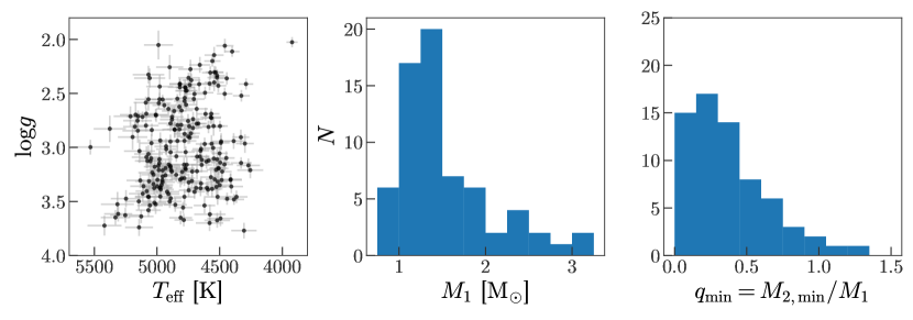
Figure 1: Left: Stellar parameters for all 234 systems used in this work. Effective temperatures, $T_{\textrm{eff}}$, and surface gravities, $\log g$, are from the APOGEE DR14 catalog. Middle: Primary masses for 68 systems with masses estimated in Ness et al. (2015). Right: Minimum mass ratios computed using primary masses from Ness et al. (2015) and companion masses estimated from orbital parameters from Price-Whelan et al. (2018).

To identify binaries, we use sources with repeat radial velocity measurements in data release 14 (DR14) of the APOGEE survey (Majewski et al. 2017; Abolfathi et al. 2017), a component of the Sloan Digital Sky Survey IV (SDSS-IV; Gunn et al. 2006; Blanton et al. 2017). A full description of our search methodology and binary star catalogs can be found in companion work (Price-Whelan et al. 2018).

Briefly, we use a custom-built Monte Carlo sampler (The Joker; Price-Whelan et al. 2017) to generate posterior samples over binary orbital parameters (period, eccentricity, etc.) for all stars with $\geq 3$ radial velocity measurements in APOGEE DR14 that pass a series of quality cuts. By making cuts on our posterior belief about the amplitude of radial velocity variations, we identified $\sim$5,000 binary star systems with at least one evolved member. However, the majority of these systems have too few radial velocity measurements to uniquely determine the binary orbital parameters.

Here, we consider only 320 binary systems for which the period and eccentricity can be uniquely determined (the “high-$K$, unimodal” sample of Price-Whelan et al. 2018). We further subselect the 234 primary stars with $\log g>2$ that pass visual inspection (from previous work, clean_flag == 0; see Section 5.2 in Price-Whelan et al. 2018). We note that because of the sparse time sampling of the APOGEE survey, we expect that our detection efficiency for high-eccentricity systems is poor, but do not expect biases for low-eccentricity systems. Figure 1, left panel, shows the stellar parameters for all 234 primary stars in the sample used in this work, middle panel shows the distribution of primary masses for the 68 systems with masses from Ness et al. (2015), and right panel shows the minimum mass ratios for the 68 systems.

Section 3 Orbital circularization of APOGEE binaries

Our sample of binaries contains primary stars with a range of stellar parameters (Figure 1), and therefore a range of expected circularization periods. Figure 2 shows orbital period and eccentricity for all systems in bins of primary surface gravity: From top left to bottom right shows bins of decreasing surface gravity, i.e. from subgiants to giant branch stars. Vertical dashed lines at $10~{}\textrm{day}$ and $100~{}\textrm{day}$ are meant as reference lines. Note the steadily increasing circularization period from top left to bottom right as the typical size of the primary increases.

To remove the dependence on the size of the primary, Figure 3 (left) shows period and eccentricity but now with periods normalized by the orbital period at which the minimum separation of the binary is equal to the surface size of the primary star,

$$P_{\textrm{surface}} =2\pi\,\left(\frac{G\,(M_{1}+M_{2})}{R_{1}^{3}}\right)^{-1/2}\,\left(1-e\right)^{-3/2}\quad.$$ (4)

We compute $P_{\textrm{surface}}$ for all systems under the following assumptions:

Primary/companion masses

Only a small fraction of the systems in our sample have measured primary masses (Figure 1) and therefore have measured (minimum) mass ratios. We make the simplifying assumption that all primary stars have masses equal to the median mass over all stars with prior mass measurements in this sample, $\textrm{med}\left(M_{1}\right)=1.36~{}\mathrm{M}_{\odot}$, and all companions have masses equal to the median over minimum companion masses, $\textrm{med}\left(M_{2,\textrm{min}}\right)=0.5~{}\mathrm{M}_{\odot}$.

Primary evolved first

We assume that the primary star (i.e. the observed star) is the first member of the binary to evolve off the main sequence.

First ascent

We assume that all primary stars are on their first ascent up the giant branch. This is motivated by the small fraction of red clump stars in our sample: Only 7 of the primaries were identified as confident red clump stars in a recent study of APOGEE DR14 evolved star (Ting et al. 2018).

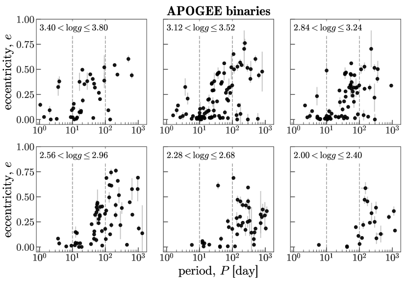
Figure 2: Orbital period and eccentricity for all systems considered in this work. Each panel shows systems in the specified bin of primary surface gravity, $\log g$. Vertical gray lines show periods of $10~{}\textrm{day}$ and $100~{}\textrm{day}$: binaries with subgiant members (top left) show circularization periods close to $10~{}\textrm{day}$, whereas binaries with RGB members (bottom right) show circularization periods close to $100~{}\textrm{day}$. Intermediate bins show steadily increasing circularization periods with decreasing $\log g$.

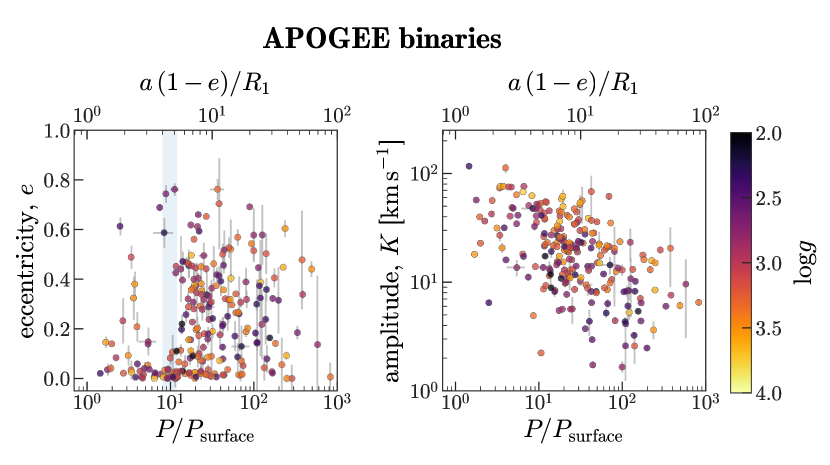
Figure 3: Left panel: Orbital period and eccentricity for binary star systems with evolved members, with period values normalized by the orbital period of a hypothetical companion that grazes the surface of each primary star, $P_{\textrm{surface}}$, assuming $M_{1}=1.36~{}\mathrm{M}_{\odot}$ and $M_{2}=0.5~{}\mathrm{M}_{\odot}$. The sharp transition from eccentric systems to almost all circular orbits at $P/P_{\textrm{surface}}\approx 10$ is likely an outcome of tidal circularization. Right panel: Normalized period and inferred radial velocity amplitude for the same systems.

Assuming that the semi-major axes of the APOGEE binaries have remained constant, and with the assumptions above, we can also compute the expected change in eccentricity, $\Delta\ln e$, for each binary (see also Figure 4 in Verbunt & Phinney 1995). As noted in Verbunt & Phinney (1995), the assumption of constant binary semi-major axis is technically incorrect, but the typical change to the semi-major axis is only between 1–10%, i.e. smaller than the uncertainty introduced in the inferred semi-major axes for our systems due to unknown inclination.

To compute $\Delta\ln e$, we use a model stellar evolution track to integrate Equation 2 up to the measured $\log g$ of each primary star. In detail, we use MESA (Paxton et al. 2011) to follow the stellar evolution of a $M_{1}=1.4~{}\mathrm{M}_{\odot}$ star with solar metallicity from the pre-main-sequence phase to the asymptotic giant branch (AGB) phase (we stop the models when they first reach $\log g=0$). For each APOGEE star, we use linear interpolation with the output of this evolutionary model to solve for the eccentricity change starting from the time the star leaves the main sequence up to the phase at which the model has the same surface gravity as is measured. We use 10,000 steps evenly spaced between these two phases and use Simpson’s rule to compute the integral.

Figure 4 shows the expected change in eccentricity plotted against the observed eccentricity for all of the APOGEE binaries. With the exception of a few outliers, systems that are predicted to have large negative changes to the log-eccentricity are circular. This confirms the conclusions of previous work based on a much smaller sample of giant star binaries (Verbunt & Phinney 1995): the theory of equilibrium tides successfully explains the observed eccentricities of close binaries with member stars that have large convective envelopes.

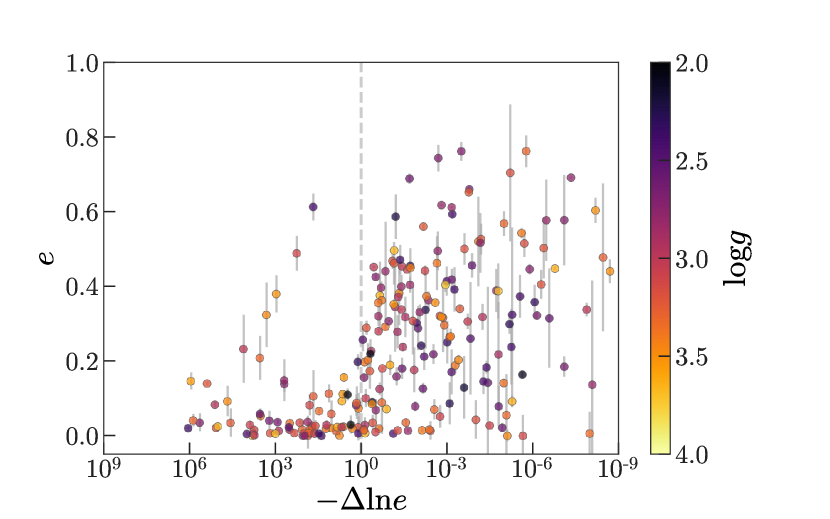
Figure 4: Predicted change in eccentricity from tidal circularization, $\Delta\ln e$, and observed eccentricity for all APOGEE binary systems. Change in eccentricity is computed assuming that the semi-major axis of the systems remain constant during eccentricity evolution, and assuming that all stars have a primary mass of $M1=1.4~{}\mathrm{M}_{\odot}$ and a companion mass of $M_{2}=0.5~{}\mathrm{M}_{\odot}$ (the median values from all systems with measured masses). Most systems with large predicted circularization have small observed eccentricities, with the exception of a few outlier systems.

Section 4 Population synthesis

To compare with the data, we generate a simulated population of binary star systems with primary stars that have similar stellar parameters (by the end of their evolution) to our sample of APOGEE system primaries. We assume simple initial binary orbital parameter distributions (i.e. in period and eccentricity) and compute the change in eccentricity and separation of the companion orbit as the primary star evolves off the main sequence.

In detail, we sample primary stellar masses, companion masses, and primary surface gravities by fitting two-component Gaussian mixture models (GMMs) to the stars in our sample with measurements of each, then re-sample using the fitted distributions. As described in previous work (Price-Whelan et al. 2018), primary mass measurements come from Ness et al. (2015), secondary (minimum) masses come from the posterior samplings over orbital parameters using APOGEE radial velocity data, and surface gravities come from the APOGEE (DR14) data reduction pipeline (García Pérez et al. 2016). In our sample, the median primary mass, companion mass, and surface gravity are $\textrm{med}\left(M_{1}\right)=1.4~{}\mathrm{M}_{\odot}$, $\textrm{med}\left(M_{2,\textrm{min}}\right)=0.4~{}\mathrm{M}_{\odot}$, and $\textrm{med}\left(\log g\right)=3.1$. We assume $M_{2}=M_{2,\textrm{min}}$ when generating companion masses.

We generate eccentricities $e$ by sampling from a truncated normal distribution with mean and standard deviation $(\mu,\sigma)=(0.4,0.3)$, truncated to the domain $[0,1]$. We note that theoretical predictions of the binary star eccentricity distribution over this period range would predict a thermalized eccentricity distribution $p(e)=2e$ (Jeans 1919), but the observed eccentricity distributions of main sequence binary star systems with periods $10<P<1000~{}\textrm{day}$ is broadly consistent with being flat for moderate eccentricities, with fewer very low and high eccentricities (Duchêne & Kraus 2013). Our comparison with this simulated population does not depend strongly on this choice of initial eccentricity distribution.

We generate initial binary orbital periods, $P$, by assuming a distribution that is uniform in $\ln P$ between $(P_{\textrm{surface}},8192)~{}\textrm{day}$. Figure 6 (left) shows the initial periods and eccentricities of the simulated systems. Markers are colored by the mass of the primary, $M_{1}$, and the size of the marker indicates the log-surface gravity, $\log g$.

To follow the stellar evolution of the primary stars, we run stellar evolution models using MESA (Paxton et al. 2011) for stars with $M=[0.8,1,1.2,1.4,1.6,1.8,2,2.5,3]~{}\mathrm{M}_{\odot}$ and solar metallicity. Figure 5 shows evolutionary tracks in surface gravity and effective temperature for each of these models. We follow the evolution from the pre-main-sequence phase until the AGB phase, but again only use the post-main-sequence evolution when evolving the orbit of the binary. At each timestep during the evolution, we output and store the standard stellar parameters along with the size and mass of the convective envelope.

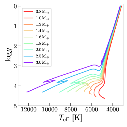
Figure 5: Evolutionary tracks of the eight stellar models we use to simulate the orbital evolution of a population of binary star systems with an evolved member. Horizontal axis shows the effective temperature, $T_{\textrm{eff}}$, and vertical axis shows the log-surface-gravity, $\log g$. Tracks are colored by the mass of the star. All models have solar metallicity.

We discretize the primary masses generated from the GMMs onto the grid of masses for which we have MESA models, then use equilibrium tide theory to compute the change in eccentricity and separation of the companion orbit. To do this, we solve the coupled differential equations Equations 2–3 up to the phase of evolution at which the stellar model has the same (or closest) surface gravity to the simulated primary star. We use the first-order Euler method with 10,000 time steps between the main sequence and the given final $\log g$ of each primary star, and use linear interpolation to interpolate the MESA output stellar parameters onto the integration grid. We assume that all stars are on their first ascent up the giant branch, which should underestimate the number of circularized systems with surface gravities $\log g\sim 2.5$ (i.e. near the red clump, where stars have already reached the tip of the giant branch). We assume that the equilibrium tides dominate the circularization process for all systems and therefore ignore the effect of “dynamical tides” (e.g., Goodman & Dickson 1998) during the main sequence phase. Finally, we assume that all of our systems are detached binaries.

Figure 6 (middle) shows the final periods and eccentricities of the simulated systems. As expected, the circularization period for higher $\log g$ systems (i.e. smaller radii, lighter markers) appears to be close to $\sim 10~{}\textrm{day}$, but the circularization period for stars with lower $\log g$ (i.e. larger radii, darker markers) is closer to $\sim 100~{}\textrm{day}$. In the right panel we normalize the orbital period by $P_{\textrm{surface}}$: This rescaling removes the dependence on primary size or $\log g$ and predicts that circularization should occur around $P/P_{\textrm{surface}}\approx 10$. The simulated systems that remain very eccentric, $e\gtrsim 0.6$, with periods $P/P_{\textrm{surface}}<10$ are likely a relic of the fact that Equations 2–3 break down when $e\sim 1$ (e.g., Hut 1981).

The sharp transition in eccentricity around $P/P_{\textrm{surface}}\approx 10$ or $a/R_{1}\approx 4$–5 observed in the sample of APOGEE binaries (Figure 3, left) is therefore qualitatively consistent with predictions from this simulated population (Figure 6, right).

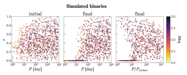
Figure 6: Simulated binary star systems with one giant star member. Points are colored by primary mass, $M_{1}$, and the size indicates the size of the star, i.e. the surface gravity $\log g$. Left: Distribution of initial orbital parameters period, $P$, and eccentricity, $e$. Middle: Final distribution of period and eccentricity after computing the change in eccentricity from evolution of the primary star. Right: Final distribution of period and eccentricity, with period normalized by $P_{\textrm{surface}}$, the period of a hypothetical, point-mass companion whose orbit grazes the surface of the primary star at pericenter.

Section 5 Discussion

5.1 Assumptions

Here we return to the assumptions made above and assess their applicability:

Primary/companion masses

Most of the systems in our sample of binaries have unmeasured primary or companion masses. In computing the normalization period, $P_{\textrm{surface}}$, and to estimate the predicted change in eccentricity, $\Delta\ln e$, we have thus made simple assumptions about the binary component masses (see Primary/companion masses above). It is therefore interesting that we see such a sharp transition in the eccentricity distribution (Figure 3, left panel), and good agreement with predictions from population synthesis and evolution of the simulated binaries (Section 4). However, this can be understood given the scaling of the circularization timescale (Equation 1) and the mass distribution of stars with measured masses (Figure 1)

Assuming a mass ratio $q=0.3$, the circularization timescale close to the circularization period, $P/P_{\textrm{surface}}\approx 10$, is very small compared to the lifetime on the giant branch for a $1.4~{}\mathrm{M}_{\odot}$ star, $t_{\textrm{circ}}\sim 10^{5}~{}\textrm{yr}\ll t_{\textrm{RGB}}\sim 10^{8}~{}\textrm{yr}$. The circularization time scales with the inverse mass ratio squared and the cubed-root of the primary mass, $t_{\textrm{circ}}\propto M_{1}^{1/3}\,\left[q\,(1+q)\right]^{-1}$: The small spread in primary masses can therefore be neglected, and variations in the mass ratio by typical factors of $\sim 2$ (Figure 1still lead to circularization timescales that are much shorter than the giant branch lifetime. For the sample of binaries considered here, the simple assumptions about primary and companion masses are therefore reasonable.

Primary evolved first

All of the binaries in our sample appear to be single-lined (from visual inspection of the APOGEE spectra). Therefore, if the companion evolved first, it would now be a stellar remnant, and its evolution as a giant would have contributed significantly to the orbital circularization. Only 4 of the systems with measured masses have minimum mass ratios above 1, indicating a possible neutron star or black hole companion. However, an unknown fraction could have white dwarf companions. Still, the majority of systems in the subset with measured masses are consistent with low-mass main sequence companions.

First ascent

As mentioned above, only 7 of the primary stars in our sample are likely red clump stars (Ting et al. 2018), and these systems all have periods between $120$–$1000~{}\textrm{day}$. This is possibly because shorter period companions would have been common-envelope when the evolved star reached the tip of the red giant branch: During this phase, rapid orbit evolution with timescales of months to years will cause engulfment and possible destruction of the companion (e.g., Nordhaus et al. 2010). We therefore consider this to be a reasonable assumption.

5.2 Exceptional systems

There are 10 systems with $e>0.1$ and $P/P_{\textrm{surface}}<6$ apparent in Figures 3 and 4. These binaries have short periods and large eccentricities that appear to be discrepant with our conclusions made about tidal circularization. Of these 10 systems, 6 have the warning flag SUSPECT_BROAD_LINES from the APOGEE pipeline, which suggests that these primary stars are either fast rotators or may contain blended light from the companion star; The inferred eccentricities for these systems may therefore be biased. In total, 39 systems distributed over the full range of periods have this warning flag. The remaining 4 systems are listed in Table 1 and warrant further study to understand why they have not circularized. One possibility is that these are actually triple systems with misaligned, long-period companions: The outer body could drive the eccentricity of the inner companion through Kozai-Lidov oscillations (Kozai 1962; Lidov 1962). Verifying this would require long-term radial velocity monitoring of these systems.

APOGEE_ID	$\log g$	$P$ [day]	$\sigma_{P}$ [day]	$e$	$\sigma_{e}$	$P/P_{\textrm{surface}}$
2M05272385+1246432	3.55	1.0529	0.0001	0.15	0.02	1.7
2M11482364+3504215	3.47	3.69	0.01	0.32	0.09	3.6
2M15042105+2700026	2.41	36.68	0.04	0.61	0.04	2.5
2M16503620-0054432	3.52	3.9823	0.0003	0.38	0.05	3.8

Table 1: Four systems that have small ratios $P/P_{\textrm{surface}}$ but still have significant eccentricities. Stellar parameters are for the primary (observed) member of the systems. In all cases, the reported uncertainties on the surface gravities are small $\sigma_{\log g}<0.1$.

Another interesting set of systems have negligible measured eccentricities with periods between $10<P<100~{}\textrm{day}$ (see top middle and right panels of Figure 2). Analogs of these systems are also seen in the simulated population in the middle panel of Figure 6: In the simulated population, these are simply systems that started with lower eccentricities and thus can evolve faster to $e\approx 0$. In the observed systems, we expect the “spur” of low-eccentricity systems at periods longer than the circularization period to be a mix of systems that started with lower eccentricity, systems in which the companion has already evolved, and a minority of red clump stars that circularized when the primary was at the tip of the giant branch.

Section 6 Conclusions

We selected binary star systems with well-determined orbital properties from a catalog of binaries identified using repeat radial velocity measurements from the APOGEE survey (Price-Whelan et al. 2018). Because of the selection function for APOGEE, the majority of these systems contain an evolved primary star that dominates the luminosity of the system, and thus these systems are predominantly single-lined spectroscopic binaries. The systems have a range of orbital periods and the primaries have a range of surface gravities, indicating that they are a mix of subgiant, giant branch, and red clump stars (Figure 1).

As has been seen in many other samples of binary star systems, we find that the short period systems have small or zero eccentricities, but above a characteristic circularization period the systems have a range of eccentricities; This circularization period depends on the stellar parameters of the primary (evolved) star in the system (Figure 2). If we normalize the orbital periods by the orbital period of the system with a hypothetical companion whose orbit just grazes the surface of the primary star (i.e. to remove the dependence on the primary star size), we find a steep transition from eccentric to circular orbits that occurs around $P/P_{\textrm{surface}}\approx 10$. This dimensionless circularization period is consistent with theoretical predictions (Figure 6): We find that the eccentricities and observed circularization periods of binary star systems with evolved members can be explained using standard tidal circularization theory for stars with significant convective envelopes (Zahn 1977, 1989; Verbunt & Phinney 1995).

The APOGEE survey was not designed to do binary star science (Majewski et al. 2017), but has enabled a number of stellar companion studies because it returns to fields as a part of its survey strategy (Troup et al. 2016; Badenes et al. 2018; Price-Whelan et al. 2018). Future data releases from APOGEE will provide more visits for current stars and nearly twice as many sources, which will allow more detailed studies of tidal circularization and other binary star phenomena. However, for bright stars, the end-of-mission data release of the Gaia mission will revolutionize binary star science by providing time-series radial velocity information for nearly 100 million stars.

References

- Abolfathi et al. (2017) Abolfathi, B., Aguado, D. S., Aguilar, G., et al. 2017, ArXiv e-prints. https://arxiv.org/abs/1707.09322
- Astropy Collaboration et al. (2013) Astropy Collaboration, Robitaille, T. P., Tollerud, E. J., et al. 2013, A&A, 558, A33, doi: 10.1051/0004-6361/201322068
- Badenes et al. (2018) Badenes, C., Mazzola, C., Thompson, T. A., et al. 2018, ApJ, 854, 147, doi: 10.3847/1538-4357/aaa765
- Blanton et al. (2017) Blanton, M. R., Bershady, M. A., Abolfathi, B., et al. 2017, AJ, 154, 28, doi: 10.3847/1538-3881/aa7567
- Bluhm et al. (2016) Bluhm, P., Jones, M. I., Vanzi, L., et al. 2016, A&A, 593, A133, doi: 10.1051/0004-6361/201628459
- Duchêne & Kraus (2013) Duchêne, G., & Kraus, A. 2013, ARA&A, 51, 269, doi: 10.1146/annurev-astro-081710-102602
- García Pérez et al. (2016) García Pérez, A. E., Allende Prieto, C., Holtzman, J. A., et al. 2016, AJ, 151, 144, doi: 10.3847/0004-6256/151/6/144
- Goodman & Dickson (1998) Goodman, J., & Dickson, E. S. 1998, ApJ, 507, 938, doi: 10.1086/306348
- Gunn et al. (2006) Gunn, J. E., Siegmund, W. A., Mannery, E. J., et al. 2006, AJ, 131, 2332, doi: 10.1086/500975
- Hunter (2007) Hunter, J. D. 2007, Computing In Science & Engineering, 9, 90
- Hut (1981) Hut, P. 1981, A&A, 99, 126
- Jeans (1919) Jeans, J. H. 1919, MNRAS, 79, 408, doi: 10.1093/mnras/79.6.408
- Kjurkchieva et al. (2017) Kjurkchieva, D., Vasileva, D., & Atanasova, T. 2017, AJ, 154, 105, doi: 10.3847/1538-3881/aa83b3
- Kozai (1962) Kozai, Y. 1962, AJ, 67, 591, doi: 10.1086/108790
- Latham et al. (2002) Latham, D. W., Stefanik, R. P., Torres, G., et al. 2002, AJ, 124, 1144, doi: 10.1086/341384
- Lidov (1962) Lidov, M. L. 1962, Planetary and Space Science, 9, 719, doi: 10.1016/0032-0633(62)90129-0
- Majewski et al. (2017) Majewski, S. R., Schiavon, R. P., Frinchaboy, P. M., et al. 2017, AJ, 154, 94, doi: 10.3847/1538-3881/aa784d
- Mathieu (2005) Mathieu, R. D. 2005, in Astronomical Society of the Pacific Conference Series, Vol. 333, Tidal Evolution and Oscillations in Binary Stars, ed. A. Claret, A. Giménez, & J.-P. Zahn, 26
- Mathieu & Mazeh (1988) Mathieu, R. D., & Mazeh, T. 1988, ApJ, 326, 256, doi: 10.1086/166087
- Mayor & Mermilliod (1984) Mayor, M., & Mermilliod, J. C. 1984, in IAU Symposium, Vol. 105, Observational Tests of the Stellar Evolution Theory, ed. A. Maeder & A. Renzini, 411
- Mazeh (2007) Mazeh, T. 2007, arXiv.org
- Meibom & Mathieu (2005) Meibom, S., & Mathieu, R. D. 2005, ApJ, 620, 970, doi: 10.1086/427082
- Meibom et al. (2006) Meibom, S., Mathieu, R. D., & Stassun, K. G. 2006, ApJ, 653, 621, doi: 10.1086/508252
- Ness et al. (2015) Ness, M., Hogg, D. W., Rix, H.-W., Ho, A. Y. Q., & Zasowski, G. 2015, ApJ, 808, 16, doi: 10.1088/0004-637X/808/1/16
- Nordhaus et al. (2010) Nordhaus, J., Spiegel, D. S., Ibgui, L., Goodman, J., & Burrows, A. 2010, MNRAS, 408, 631, doi: 10.1111/j.1365-2966.2010.17155.x
- Paxton et al. (2011) Paxton, B., Bildsten, L., Dotter, A., et al. 2011, ApJS, 192, 3, doi: 10.1088/0067-0049/192/1/3
- Pérez & Granger (2007) Pérez, F., & Granger, B. E. 2007, Computing in Science and Engineering, 9, 21, doi: 10.1109/MCSE.2007.53
- Price-Whelan et al. (2017) Price-Whelan, A. M., Hogg, D. W., Foreman-Mackey, D., & Rix, H.-W. 2017, ApJ, 837, 20, doi: 10.3847/1538-4357/aa5e50
- Price-Whelan et al. (2018) Price-Whelan, A. M., Hogg, D. W., & Rix, H.-W. e. a. 2018, AAS journals, submitted
- Shporer et al. (2016) Shporer, A., Fuller, J., Isaacson, H., et al. 2016, ApJ, 829, doi: 10.3847/0004-637X/829/1/34
- Ting et al. (2018) Ting, Y.-S., Hawkins, K., & Rix, H.-W. 2018, ArXiv e-prints. https://arxiv.org/abs/1803.06650
- Troup et al. (2016) Troup, N. W., Nidever, D. L., De Lee, N., et al. 2016, AJ, 151, 85, doi: 10.3847/0004-6256/151/3/85
- Van der Walt et al. (2011) Van der Walt, S., Colbert, S. C., & Varoquaux, G. 2011, Computing in Science & Engineering, 13, 22, doi: http://dx.doi.org/10.1109/MCSE.2011.37
- Verbunt & Phinney (1995) Verbunt, F., & Phinney, E. S. 1995, A&A, 296, 709
- Zahn (1977) Zahn, J.-P. 1977, A&A, 57, 383
- Zahn (1989) —. 1989, A&A, 220, 112
- Zahn (2008) Zahn, J.-P. 2008, in EAS Publications Series, Vol. 29, EAS Publications Series, ed. M.-J. Goupil & J.-P. Zahn, 67–90