Dimensionally regularized Boltzmann-Gibbs Statistical Mechanics and two-body Newton’s gravitation

Abstract

It is believed that the canonical gravitational partition function $Z$ associated to the classical Boltzmann-Gibbs (BG) distribution $\frac{e^{-\beta H}}{{\cal Z}}$ cannot be constructed because the integral needed for building up $Z$ includes an exponential and thus diverges at the origin. We show here that, by recourse to 1) the analytical extension treatment obtained for the first time ever, by Gradshteyn and Rizhik, via an appropriate formula for such case and 2) the dimensional regularization approach of Bollini and Giambiagi’s (DR), one can indeed obtain finite gravitational results employing the BG distribution. The BG treatment is considerably more involved than its Tsallis counterpart. The latter needs only dimensional regularization, the former requires, in addition, analytical extension. PACS: 05.20.-y, 02.10.-v
KEYWORDS: Boltzmann-Gibbs distribution, divergences, dimensional regularization, specific heat.

1 Introduction

DR [1, 2] constitutes one of the greatest advances in the theoretical physics of the last 45 years, with applications in several branches of physics (see, for instance, [3]-[56].

It is commonly believed that the classical Boltzmann-Gibbs (BG) probability distribution can not yield finite results because the associated partition function ${\cal Z}$ in $\nu$ dimensions diverges [57, 59], as one has ($m$ and $M$ are the masses involved, $G$ the gravitation constant, $\beta$ the inverse temperature, and $x$-$p$ the phase-space coordinates)

$${\cal Z}_{\nu}=\int\limits_{M}e^{-\beta\left(\frac{p^{2}}{2m}-\frac{GmM}{r}\right)}d^{\nu}xd^{\nu}p,$$ (1.1)

with a positive exponential. However, such belief does not take into account the possibility of analytical extensions, that would take care of divergences, e.g., at the origin.

It has been shown in Ref.[60], for first time ever, that ${\cal Z}$ can be calculated for Tsallis entropy using the 40-years old DR technique.

Why are we insisting on this issue if it has been already solved?. The issue needs revisiting because it does not work for $q=1$, that is, for the Boltzmann-Gibbs statistics, due to the fact that we there face an exponential divergence. In this paper we report on how to overcome this problem by judicious use of an appropriate combination of DR plus analytical extension. This produces the first ever ´BG partition function for the two-body gravitational problem. We remark that the N-body gravitational problem has not yet been solved and constitutes a frontier research problem in Celestial Mechanics.

It is well known that, at a quantum field theory level, DR can not cope with the gravitational field, since it is non-renormalizable. Our present challenge is quite different, though, because we deal with Newton’s gravity at a classical level.

2 Analytic extension

In this section we collect a set of mathematical results that will be needed afterwards. This Section may be omitted at a first reading. We must now keep in mind that we are dealing with the integral of an exponentially increasing function given by (1.1). We resort to Ref. [61], and following it we consider a useful integral, that will greatly help with our inquires, after judicious specializations of it. This integral reads

$$\int\limits_{0}^{\infty}x^{\nu-1}(x+\gamma)^{\mu-1}e^{-\frac{\beta}{x}}dx=\beta^{\frac{\nu-1}{2}}\gamma^{\frac{\nu-1}{2}+\mu}\Gamma(1-\mu-\nu)e^{\frac{\beta}{2\gamma}}W_{\frac{\nu-1}{2}+\mu,-\frac{\nu}{2}}\left(\frac{\beta}{\gamma}\right),$$ (2.1)

$|\arg(\gamma)|<\pi$, $\Re(1-\mu-\nu)>0$, where $W$ is one of the two Whittaker functions. One does not require $\Re\beta>0$, as emphasized by Gradshteyn and Rizhik [61] (see figure in page 340, eq. (7), called ET II 234(13)a, where reference is made to [62] (Caltech’s Bateman Project). The last letter ”a” indicates that analytical extension has been performed. Choosing $\mu=1$ above we find

$$\int\limits_{0}^{\infty}x^{\nu-1}e^{-\frac{\beta}{x}}dx=\beta^{\frac{\nu-1}{2}}\gamma^{\frac{\nu+1}{2}}\Gamma(-\nu)e^{\frac{\beta}{2\gamma}}W_{\frac{\nu+1}{2},-\frac{\nu}{2}}\left(\frac{\beta}{\gamma}\right),$$ (2.2)

valid for $\nu\neq 0,-1,-2,-3,.....$ Additionally [61],

$$W_{\frac{\nu+1}{2},-\frac{\nu}{2}}\left(\frac{\beta}{\gamma}\right)=M_{\frac{\nu+1}{2},\frac{\nu}{2}}\left(\frac{\beta}{\gamma}\right)=\left(\frac{\beta}{\gamma}\right)^{\frac{\nu+1}{2}}e^{-\frac{\beta}{2\gamma}},$$ (2.3)

where $M$ stands for the other Whittaker function. Thus,

$$\int\limits_{0}^{\infty}x^{\nu-1}e^{-\frac{\beta}{x}}dx=\beta^{\nu}\Gamma(-\nu)$$ (2.4)

an integral that can be evaluated for all $\nu=1,2,3,....$ by recourse to the dimensional regularization technique [1, 2]. Changing now $\beta$ by $-\beta$ in (2.1) we have

$$\int\limits_{0}^{\infty}x^{\nu-1}(x+\gamma)^{\mu-1}e^{\frac{\beta}{x}}dx=(-\beta)^{\frac{\nu-1}{2}}\gamma^{\frac{\nu-1}{2}+\mu}\Gamma(1-\mu-\nu)e^{-\frac{\beta}{2\gamma}}W_{\frac{\nu-1}{2}+\mu,-\frac{\nu}{2}}\left(-\frac{\beta}{\gamma}\right).$$ (2.5)

Once again we choose $\mu=1$ and have

$$\int\limits_{0}^{\infty}x^{\nu-1}e^{\frac{\beta}{x}}dx=(-\beta)^{\frac{\nu-1}{2}}\gamma^{\frac{\nu+1}{2}}\Gamma(-\nu)e^{-\frac{\beta}{2\gamma}}W_{\frac{\nu+1}{2},-\frac{\nu}{2}}\left(-\frac{\beta}{\gamma}\right),$$ (2.6)

valid for $\nu\neq 0,-1,-2,-3,.....$ One now faces

$$W_{\frac{\nu+1}{2},-\frac{\nu}{2}}\left(-\frac{\beta}{\gamma}\right)=M_{\frac{\nu+1}{2},\frac{\nu}{2}}\left(-\frac{\beta}{\gamma}\right)=\left(-\frac{\beta}{\gamma}\right)^{\frac{\nu+1}{2}}e^{\frac{\beta}{2\gamma}},$$ (2.7)

and

$$\int\limits_{0}^{\infty}x^{\nu-1}e^{\frac{\beta}{x}}dx=(-\beta)^{\nu}\Gamma(-\nu)$$ (2.8)

tantamount to changing $\beta$ by $-\beta$ in (2.4). We have thus shown a rather interesting fact. Restriction of analytical extension (AE) of (2.1) equals AE of the restriction of that relation. This reconfirms that Gradshteyn and Rizhik’s AE is indeed correct. Eq. (2.8) displays a cut at $\Re\beta>0$. One can then choose $(-\beta)^{\nu}=e^{i\pi\nu}\beta^{\nu}$, $(-\beta)^{\nu}=e^{-i\pi\nu}\beta^{\nu}$, or $(-\beta)^{\nu}=\cos(\pi\nu)\beta^{\nu}$. We select the last possibility and obtain

$$\int\limits_{0}^{\infty}x^{\nu-1}e^{\frac{\beta}{x}}dx=\cos(\pi\nu)\beta^{\nu}\Gamma(-\nu),$$ (2.9)

an important result that we will use in Section 3. From [61] we note that

$$\int\limits_{0}^{\infty}x^{\nu-1}e^{-\beta x^{2}-\gamma x}dx=(2\beta)^{-\frac{\nu}{2}}\Gamma(\nu)e^{\frac{\gamma^{2}}{8\beta}}D_{-\nu}\left(\frac{\gamma}{\sqrt{2\beta}}\right),$$ (2.10)

where $D$ is the parabolic-cylinder function. Selecting $\gamma=0$ one finds

$$\int\limits_{0}^{\infty}x^{\nu-1}e^{-\beta x^{2}}dx=(2\beta)^{-\frac{\nu}{2}}\Gamma(\nu)D_{-\nu}(0).$$ (2.11)

Since

$$D_{-\nu}(0)=\frac{2^{-\frac{\nu}{2}}\sqrt{\pi}}{\Gamma\left(\frac{\nu+1}{2}\right)},$$ (2.12)

we find

$$\int\limits_{0}^{\infty}x^{\nu-1}e^{-\beta x^{2}}dx=\frac{2^{-\nu}\beta^{-\frac{\nu}{2}}\sqrt{\pi}\;\Gamma(\nu)}{\Gamma\left(\frac{\nu+1}{2}\right)},$$ (2.13)

another important result that we will use in Section 3.

3 The $\nu$-dimensional BG distribution

The BG partition function ${\cal Z}_{\nu}$ is

$${\cal Z}_{\nu}=\int\limits_{M}e^{-\beta\left(\frac{p^{2}}{2m}-\frac{GmM}{r}\right)}d^{\nu}xd^{\nu}p.$$ (3.1)

For effecting the integration process one uses hyper-spherical coordinates and two integrals, each in $\nu$ dimensions. The corresponding change of variables is defined as

$$x_{1}=r\cos\theta_{1}$$

$$x_{2}=r\sin\theta_{1}\cos\theta_{2}$$

$$x_{3}=r\sin\theta_{1}\sin\theta_{2}\cos\theta_{3}$$

$$\cdot$$

$$\cdot$$

$$x_{\nu-1}=r\sin\theta_{1}......\sin\theta_{\nu-2}\cos\theta_{\nu-1}$$

$$x_{\nu}=\sin\theta_{1}......\sin\theta_{\nu-1}\sin\theta_{\nu-1},$$ (3.2)

where $0\leq\theta_{j}\leq\pi$, $1\leq j\leq\nu-2$, and $0\leq\theta_{\nu-1}\leq 2\pi$. The integration on the angular variables ($\Omega_{\nu}=(\theta_{1},\theta_{2},...,\theta_{\nu-1})$) yields as a result

$$\int\limits_{\Omega_{\nu}}d\Omega_{\nu}=\left[\frac{2\pi^{\frac{\nu}{2}}}{\Gamma\left(\frac{\nu}{2}\right)}\right]$$ (3.3)

Ones is left then with just two radial coordinates (one in $r-$ space and the other in $p-$ space) and $2(\nu-1)$ angles. Accordingly,

$${\cal Z}_{\nu}=\left[\frac{2\pi^{\frac{\nu}{2}}}{\Gamma\left(\frac{\nu}{2}\right)}\right]^{2}\iint\limits_{0}^{\infty}(rp)^{\nu-1}e^{-\beta\left(\frac{p^{2}}{2m}-\frac{GmM}{r}\right)}dr\;dp.$$ (3.4)

Now, using (2.9) for $\int\limits_{0}^{\infty}r^{\nu-1}e^{\beta\frac{GmM}{r}}dr$ and (2.13) for $\int\limits_{0}^{\infty}p^{\nu-1}e^{-\beta\frac{p^{2}}{2m}}dp$ we obtain

$${\cal Z}_{\nu}=4\sqrt{\pi}\cos(\pi\nu)\left(\frac{\pi^{2}\beta G^{2}m^{3}M^{2}}{2}\right)^{\frac{\nu}{2}}\frac{\Gamma(\nu)\Gamma(-\nu)}{\left[\Gamma\left(\frac{\nu}{2}\right)\right]^{2}\Gamma\left(\frac{\nu+1}{2}\right)}.$$ (3.5)

From (3.5) one gathers that poles appear for any dimension $\nu$, $\nu=3$ included. Thus, appeal to dimensional regularization (DR) will be mandatory. To this effect we will use in Section 4 the DR-Bollini @ Giambiagi’s technique’s generalization given in [2].

Before, we still need an expression for the mean energy

$$<{\cal U}>_{\nu}=\frac{1}{{\cal Z}_{\nu}}\int\limits_{M}e^{-\beta\left(\frac{p^{2}}{2m}-\frac{GmM}{r}\right)}\left(\frac{p^{2}}{2m}-\frac{GmM}{r}\right)d^{\nu}xd^{\nu}p.$$ (3.6)

Appealing to the hyper-spherical coordinates previously mentioned we obtain for $<{\cal U}>_{\nu}$

$$<{\cal U}>_{\nu}=\frac{1}{{\cal Z}_{\nu}}\left[\frac{2\pi^{\frac{\nu}{2}}}{\Gamma\left(\frac{\nu}{2}\right)}\right]^{2}\iint\limits_{o}^{\infty}e^{-\beta\left(\frac{p^{2}}{2m}-\frac{GmM}{r}\right)}\left(\frac{p^{2}}{2m}-\frac{GmM}{r}\right)p^{\nu-1}r^{\nu-1}dp\;dr.$$ (3.7)

At this stage we use again (2.9) and (2.13), which yields for the mean energy

$$<U>_{\nu}=\frac{1}{{\cal Z}_{\nu}}\frac{\sqrt{\pi}}{\beta}\cos(\pi\nu)\left(\frac{\pi^{2}\beta G^{2}m^{3}M^{2}}{2}\right)^{\frac{\nu}{2}}\otimes$$

$$\left[\frac{\Gamma(\nu+2)\Gamma(-\nu)}{\left[\Gamma\left(\frac{\nu}{2}\right)\right]^{2}\Gamma\left(\frac{\nu+3}{2}\right)}+4\frac{\Gamma(\nu)\Gamma(1-\nu)}{\left[\Gamma\left(\frac{\nu}{2}\right)\right]^{2}\Gamma\left(\frac{\nu+1}{2}\right)}\right].$$ (3.8)

4 The 3D regularized BG distribution

We go back to (3.5). The idea it to work out the ensuing dimensional regularization (DR) process. If we have, for instance, an expression $F(\nu)$ that diverges, say, for $\nu=3$, our Bollini-Giambiagi’s DR generalized approach consists in performing the Laurent-expansion of $F$ around $\nu=3$ and select afterwards, as the physical result for $F$, the $\nu=3$-independent term in the expansion. The justification for such a procedure is clearly explained in [2].

In our case, the corresponding Laurent expansion in the variable $\nu$ around $\nu=3$ is

$${\cal Z}_{\nu}=-\frac{2}{3\sqrt{\pi}}\frac{(2\pi^{2}\beta G^{2}m^{3}M^{2})^{\frac{3}{2}}}{3(\nu-3)}-\frac{1}{3\sqrt{\pi}}(2\pi^{2}\beta G^{2}m^{3}M^{2})^{\frac{3}{2}}\otimes$$

$$\left[\ln\left(2\pi^{2}\beta G^{2}m^{3}M^{2}\right)-\boldsymbol{C}-\frac{17}{3}\right]+\sum\limits_{s=1}^{\infty}a_{s}(\nu-3)^{s}.$$ (4.1)

where $\boldsymbol{C}$ is Euler’s constant. We clearly see that ${\cal Z}_{\nu}$ diverges at $\nu=3$. By definition (and this is the essence of DR), the independent $(\nu-3)$-term in the ${\cal Z}_{\nu}$-Laurent expansion yields the physical value of the ${\cal Z}$. Thus,

$${\cal Z}=\frac{1}{3\sqrt{\pi}}(2\pi^{2}\beta G^{2}m^{3}M^{2})^{\frac{3}{2}}\left[\frac{17}{3}-\boldsymbol{C}-\ln\left(8\pi^{2}\beta G^{2}m^{3}M^{2}\right)\right].$$ (4.2)

Since ${\cal Z}$ must be positive, one faces a temperature-lower bound

$$T>\frac{e^{-\frac{17}{3}-\boldsymbol{C}}}{k_{B}}8\pi^{2}G^{2}m^{3}M^{2}.$$ (4.3)

Similarly, from (3.8), we have for $<{\cal U}>$ the Laurent expansion

$${\cal Z}<{\cal U}>_{\nu}=\frac{8}{\sqrt{\pi}\beta(\nu-3)}\left(\frac{\pi^{2}\beta G^{2}m^{3}M^{2}}{2}\right)^{\frac{3}{2}}+\frac{8}{\sqrt{\pi}\beta}\left(\frac{\pi^{2}\beta G^{2}m^{3}M^{2}}{2}\right)^{\frac{3}{2}}\otimes$$

$$\left[\frac{1}{2}\ln\left(\frac{\pi^{2}\beta G^{2}m^{3}M^{2}}{2}\right)+2\ln 2-\frac{\boldsymbol{C}}{2}-\frac{5}{2}\right]+\sum\limits_{s=1}^{\infty}a_{s}(\nu-3)^{s}.$$ (4.4)

where ${\cal Z}$ is given by (4.2). Accordingly, the $(\nu-3)$-independent term is the physical value of $<{\cal U}>$

$$<{\cal U}>=\frac{1}{{\cal Z}}\frac{8}{\sqrt{\pi}\beta}\left(\frac{\pi^{2}\beta G^{2}m^{3}M^{2}}{2}\right)^{\frac{3}{2}}\left[\frac{1}{2}\ln\left(\frac{\pi^{2}\beta G^{2}m^{3}M^{2}}{2}\right)+2\ln 2-\frac{\boldsymbol{C}}{2}-\frac{5}{2}\right],$$ (4.5)

Replacing here the physical value of ${\cal Z}$ given by (4.2) we now obtain

$$<{\cal U}>=-\frac{3}{2\beta}\frac{\ln\left(\pi^{2}\beta G^{2}m^{3}M^{2}\right)+3\ln 2-\boldsymbol{C}-5}{\ln\left(\pi^{2}\beta G^{2}m^{3}M^{2}\right)+\ln 8-\boldsymbol{C}-\frac{17}{3}}.$$ (4.6)

5 Specific Heat

We are now in possession, for the first time ever, of a canonical gravitational mean energy function. Thus, we use it for evaluating the specific heat

${\cal C}=\frac{\partial<{\cal U}>}{\partial T}$. Thus, we obtain

$${\cal C}=\frac{3k}{2}\frac{\ln(\pi^{2}\beta G^{2}m^{3}M^{2})+3\ln 2-6--\boldsymbol{C}}{\frac{17}{3}+\boldsymbol{C}-\ln(2\pi^{2}\beta G^{2}m^{3}M^{2})-\ln 2}-$$

$$\frac{3k}{2}\frac{\ln(16\pi^{2}\beta G^{2}m^{3}M^{2})+3\ln 2-5-\boldsymbol{C}}{\left[\frac{17}{3}+\boldsymbol{C}-\ln(2\pi^{2}\beta G^{2}m^{3}M^{2})-\ln 2\right]^{2}}$$ (5.1)

Figs. 1 depict the specific heat corresponding to Eq. (5.1). We call $E=G^{2}m^{3}M^{2}$ with $m<<<M$. We express quantities in $k_{B}T/E$-units. The specific heat is negative, as befits gravitation [57]. Indeed, such an occurrence has been associated to self-gravitational systems [57]. Thirring has magnificently illustrated on negative heat capacities [58]. In turn, Verlinde has associated this type of systems to an entropic force [63]. It is natural to conjecture then that such a force may appear at the energy-associated poles. Notice also that temperature ranges are restricted. There is a $T-$lower bound.

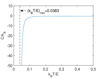
Figure 1: Specific heat versus $k_{B}T/E$

6 Discussion

It is commonly believed that the partition function ${\cal Z}$ associated to a Boltzmann-Gibbs (BG) probability distribution diverges [57, 59]. However, such belief does not take into account the possibility of analytical extensions. We have conclusively shown here that analytical extension coupled to dimensional regularization (DR), allows one to obtain a finite gravitational BG partition function.

We acknowledge the fact that the classical gravitational problem has wider horizons, that were not touched here. Our contribution was just that of providing a finite partition function for the two-body gravitational problem.

A special point to be remarked is the following. The statistical gravitational problem is one in which the BG treatment is considerably more involved than its Tsallis counterpart. The latter needs only dimensional regularization, the former requires, in addition, analytical extension.

Note that dealing with Newton’s gravity with Tsallis’s q-statistics plus the DR also solves the problem of obtaining a for $q=4/3$ [60] . To do the same with BG-statistics demands, in addition, analytical extension. One may wonder what is the role played by the parameter $q$. We have shown in the references given in [64] that $q$ is an indicator of the energy-amount involved in physical processes related to resonances and Quantum Field Theory (QFT). The greater is the q-value, the larger the value of the energy involved in the process. According to results of the Alice experiment of the LHC [64], one finds that non-linear quantum fields would manifest themselves around 15 TEVs and that these fields would eventually correspond to an approximate value of q = 1.5. The value $q=1$ would correspond the usual, linear QFT.

One might perhaps conjecture that for Newton’s gravity (NG) something similar happens. For usual energies, the NG-statistical treatment should be the BG one. At bigger energies, one may better resort to Tsallis statistics. A relevant example is given in Ref. [65].

References

- [1] C. G. Bollini and J. J. Giambiagi, Phys. Lett. B 40, 566 (1972); Il Nuovo Cim. B 12, 20 (1972); C. G. Bollini and J.J Giambiagi, Phys. Rev. D 53, 5761 (1996); W. Bietenholz, L. Prado, Physics Today 67, 38 (2014);
- [2] A. Plastino, M. C. Rocca: ”Quantum Field Theory, Feynman and Wheeler Propagators and Dimensional Regularization in Configuration Space”. ArXiv:1708.04506.
- [3] D. Berenstein and A. Miller: Phys. Rev. D 90 (2014), 086011.
- [4] D. Anselmi: Phys. Rev. D 89 (2014), 125024.
- [5] P. Jaranowski and G. Schäfer: Phys. Rev. D 87 (2013), 081503(R).
- [6] T. Inagaki, D. Kimura, H. Kohyama, and A. Kvinikhidze: Phys. Rev. D 86 (2012), 116013.
- [7] J. Qiu: Phys. Rev. D 77 (2008), 125032.
- [8] L. Blanchet, T. Damour, G. Esposito-Farèse, and B. R. Iyer: Phys. Rev. D 71 (2005), 124004.
- [9] F. Bastianelli, O. Corradini, and A. Zirotti: Phys. Rev. D 67 (2003), 104009.
- [10] D. Lehmann and G. Prézeau: Phys. Rev. D 65 (2001), 016001.
- [11] A. P. Baêta Scarpelli, M. Sampaio, and M. C. Nemes: Phys. Rev. D 63 (2001), 046004.
- [12] E. Braaten and Yu-Qi Chen: Phys. Rev. D 55 (1997), 7152.
- [13] J. Smith and W. L. van Neerven EPJ C 40 (2005), 199.
- [14] J. F. Schonfeld EPJ C 76 (2016), 710.
- [15] C. Gnendiger et al.: EPJ C 77 (2017), 471.
- [16] P. Arnold, Han-Chih Chang and S. Iqbal: JHEP 100 (2016).
- [17] I. AravE, Y. Oz and A. Raviv-Moshe: JHEP 88 (2017).
- [18] C. Anastasiou, S. Buehler, C. Duhr and F. Herzog: JHEP 62 (2012).
- [19] F. Niedermayer and P. Weisz: JHEP 110 (2016).
- [20] C. Coriano, L. Delle Rose, E. Mottolaand M. Serino: JHEP 147 (2012).
- [21] F. Dulat, S. Lionetti, B. Mistlberger,A. Pelloni and C. Specchia: JHEP 17 (2017).
- [22] T. Gehrmann and N. Greiner: JHEP 50 (2010).
- [23] T.Lappia and R.Paatelainena: Ann. of Phys. 379 (2017), 34.
- [24] S.Grooteab, J.G.Körner and A.A.Pivovarov: Ann. of Phys. 322 (2007), 2374.
- [25] N.C.Tsamis and R.P.Woodard: Ann. of Phys. 321 (2006), 875.
- [26] S. Krewaland and K. Nakayama: Ann. of Phys. 216 (1992), 210.
- [27] L. Rosen and J. D. Wright Comm. Math. Phys. 134 (1990), 433.
- [28] F. David Comm. Math. Phys. 81 (1981), 149.
- [29] P. Breitenlohner and D. Maison Comm. Math. Phys. 52 (1977), 11.
- [30] S. Teber and A. V. Kotikov: EPL 107 (2014), 57001.
- [31] H. Fujisaki: EPL 28 (1994), 623.
- [32] M. W. Kalinowski, M. Seweryński and L. Szymanowski: JMP 24 (1983), 375.
- [33] R. Contino and A. Gambassi: JMP 44 (2003), 570.
- [34] M. Dutsch, K. Fredenhagen, K. J. Keller and K. Rejzner3: JMP 55 (2014), 122303.
- [35] T. Nguyena: JMP 57 (2016), 092301.
- [36] J. Ben Geloun and R. Toriumi: JMP 56 (2015), 093503.
- [37] J. Ben Geloun and R. Toriumi: J. Phys. A 45 (2012), 374026.
- [38] B. Mutet, P. Grange and E. Werner: J. Phys. A 45 (2012), 315401.
- [39] M. C Abbott and P. Sundin: J. Phys. A 45 (2012), 025401.
- [40] T Fujihara et al.: J. Phys. A 39 (2008), 6371.
- [41] Silke Falk et al.: J. Phys. A 43 (2010), 035401.
- [42] Germán Rodrigo et al.: J. Phys. G 25 (1999), 1593.
- [43] B. M. Pimentel and J. L. Tomazelli: J. Phys. G 20 (1994), 845.
- [44] A. Khare: J. Phys. G 3 (1977), 1019.
- [45] J. C. D’Cruz: J. Phys. G 1 (1975), 151.
- [46] R. Sepahv and S. Dadfar: Nuc. Phys. A 960 (2017), 36.
- [47] J. V. Steele and R. J. Furnstahl: Nuc. Phys. A 630 (1998), 46.
- [48] D. R. Phillips, S. R. Beane and T. D. Cohena: Nuc. Phys. A 631 (1998), 447.
- [49] A. J. Stoddart and R. D. Viollier: Nuc. Phys. A 532 (1991), 657.
- [50] E. Panzer: Nuc. Phys. B 874 (2013), 567.
- [51] R. N. Lee, A. V. Smirnov and and V. A. Smirnov: Nuc. Phys. B 856 (2012), 95.
- [52] A. P. Isaev: Nuc. Phys. B 662 (2003), 461.
- [53] J. M. Campbell, E. W. N. Glover and D. J. Miller: Nuc. Phys. B 498 (1997), 397.
- [54] C. J. Yang, M. Grasso, X. Roca-Maza, G. Colo, and K. Moghrabi: Phys. Rev. C 94 (2016), 034311.
- [55] K. Moghrabi and M. Grasso: Phys. Rev. C 86 (2012), 044319.
- [56] D. R. Phillips, I. R. Afnan, and A. G. Henry-Edwards: Phys. Rev. C 61 (2000), 044002.
- [57] D. Lynden-Bell, R. M. Lynden-Bell, Mon. Not. R. Astron. Soc. 181 (1977), 405.
- [58] W. Thirring, Z. Phys. 235 (1970), 339; Paths of Discovery, Pontifical Academy of Sciences, Acta 18, Vatican City 2006.
- [59] T. Padmanabhan, Physics Reports 188 (1990), 285; T.Padmanabhan in Dynamics and Thermodynamics of Systems with Long Range Interactions Eds: T.Dauxois, S.Ruffo, E.Arimondo, M.Wilkens; Lecture Notes in Physics (Springer, Berlin, 2002); [astro-ph/0206131]; T. Padmanabhan, Theoretical Astrophysics, Vol.I: Astrophysical Processes (Cambridge University Press, Cambridge, 2000), chapter 10; J. Binney and S. Tremaine, Galactic Dynamics (Princeton University Press, New Jersey, 1987).
- [60] J. D. Zamora, M. C. Rocca, A. Plastino, G. L. Ferri, Physica A (2018), https://doi.org/10.1016/j.physa.2018.01.018
- [61] I. S. Gradshteyn and I. M. Rizhik, Table of Integrals Series and Products. Academic Press, NY (1965).
- [62] A. Erdelyi, Tables of Integral Tranforms, Vol. II (Mc Graw Hill, NY, 1954).
- [63] E. Verlinde, arXiv:1001.0785 [hep-th]; JHEP 04 (2011), 29.
- [64] A. Plastino, M.C. Rocca: EPL 118 (2017), 61004; A. Plastino, M.C. ROCCA: EPL 116 (2016), 41001; A. Plastino, M. C. Rocca, G. L. Ferri, D. J. Zamora: NPA 955 (2016), 16; A. Plastino, M. C. Rocca: NPA 948 (2016), 19.
- [65] A. R. Plastino, A. Plastino: PLA 174 (1993), 384.