Generalized permutohedra in the kinematic space

Abstract.

In this note, we study the permutohedral geometry of the poles of a certain differential form introduced in recent work of Arkani-Hamed, Bai, He and Yan. There it was observed that the poles of the form determine a family of polyhedra which have the same face lattice as that of the permutohedron. We realize that family explicitly, proving that it in fact fills out the configuration space of a particularly well-behaved family of generalized permutohedra, the zonotopal generalized permutohedra, that are obtained as the Minkowski sums of line segments parallel to the root directions $e_{i}-e_{j}$.

Finally we interpret Mizera’s formula for the biadjoint scalar amplitude $m(\mathbb{I}_{n},\mathbb{I}_{n})$, restricted to a certain dimension $n-2$ subspace of the kinematic space, as a sum over the boundary components of the standard root cone, which is the conical hull of the roots $e_{1}-e_{2},\ldots,e_{n-2}-e_{n-1}$.

1. The kinematic space

Let $I=\{a,1,2,\ldots,n-1,n,b\}$, where $a,b$ are auxiliary indices.

Definition 1.

Define the kinematic space to be the subspace of $\mathbb{R}^{(n+2)^{2}}$,

$$\mathcal{K}^{n}=\left\{(s_{ij})\in\mathbb{R}^{(n+2)^{2}}:s_{ii}=0,\ s_{ij}=s_{ji},\ i,j\in I,\text{ and }\sum_{j\in I:j\not=i}s_{ij}=0\text{ for all }i\in I\right\}.$$

Denote by $\mathcal{K}^{n}(\mathcal{D})$ the intersection in $\mathcal{K}^{n}$ of the $\binom{n}{2}$ affine hyperplanes $s_{ij}=-c_{ij}$ for all $1\leq i<j\leq n$ for given constants $\mathcal{D}=(c_{ij})$ with $c_{ij}\geq 0$.

We denote

$$s_{J}=\sum_{i,j\in J:\ i<j}s_{ij}$$

and

$$s_{J_{1}|J_{2}}=\sum_{(i,j)\in J_{1}\times J_{2}}s_{ij}$$

for (nonempty) subsets $J,J_{1},J_{2}$ of $I$, where $J_{1}\cap J_{2}=\emptyset$. Let us adopt the natural convention that $s_{J}=0$ for any singlet $J=\{j\}$.

Note that $\dim(\mathcal{K}^{n})=\binom{n+2}{2}-(n+2)=\frac{(n+2)(n-1)}{2}$, and

$$\dim(\mathcal{K}^{n}(\mathcal{D}))=\binom{n+2}{2}-(n+2)-\binom{n}{2}=n-1.$$

In [2], after adjusting the notation, the inequalities corresponding to the facets of a polyhedral cone were given as

$$s_{aJ}=s_{aj_{1}\cdots j_{k}}\geq 0,$$

as $J$ ranges over all $2^{n}-2$ proper nonempty subsets of $\{1,\ldots,n\}$.

Remark 2.

The coordinates $s_{ij}$ actually have an essential structure which is not needed explicitly for our results. They are called generalized Mandelstam invariants. They are constructed from momentum vectors $p_{1},\ldots,p_{n+2}$ of a system of particles satisfying momentum conservation $\sum_{i=1}^{n+2}p_{i}=0$, in spacetime of dimension $D\geq n+1$ with the Minkowski inner product, and are defined by $s_{ij}=(p_{i}+p_{j})^{2}=2p_{i}\cdot p_{j}$, due the assumption that particles are massless, that is $p_{i}\cdot p_{i}=0$, where we are using the notation $p^{2}:=p\cdot p$ for any linear combination of momentum vectors $p$.

Remark 3.

It is worth pointing out that, as an $\mathfrak{S}_{n+2}$-module, $\mathcal{K}^{n}$ is irreducible, and is isomorphic to to $V_{(n,2)}$, that is the $\frac{(n+2)(n-1)}{2}$-dimensional irreducible representation labeled by the partition $(n,2)$ of $n+2$.

In Theorem 8 we derive and use the formula for the characteristic function of the intersection of the set of affine hyperplanes $s_{ij}=-c_{ij}$ with the region determined by the set of $2^{n}-2$ inequalities

$$s_{aJ}=s_{aj_{1}\cdots j_{k}}\geq 0,$$

where $J$ varies over all nonempty proper subsets of $\{1,\ldots,n\}$, to show in particular that each such intersection is a zonotopal generalized permutohedron, and all zonotopal generalized permutohedra are obtained in this way.

It may seem surprising a priori that the canonical form for the permutohedron, on the kinematic space, as in [2], would encode so specialized a family as the zonotopal generalized permutohedra. However, it is also a much studied and indeed relatively well-understood special case which already has some powerful results and techniques that immediately become available. For example, consider this: there is a certain quasi-symmetric function invariant of the normal cone of a generalized permutohedron, see Section 9.1 of [4]. It turns out for the zonotopal generalized permutohedra, this quasi-symmetric function coincides with Stanley’s chromatic symmetric function. For other generalized permutohedra this invariant is likely to be only a quasisymmetric function; indeed, this happens already for the equilateral triangle.

While it is not true for general graphs, it is currently being studied whether Stanley’s chromatic symmetric function can distinguish those zonotopal generalized permutohedra which are encoded by trees. This question was originally posed by Stanley in [21].

2. Main result

Let us comment briefly on how we resolve and future-proof some potentially conflicting conventions. In [2], $(n-3)$-dimensional generalized permutohedra were embedded in an ambient space of dimension $n-2$ in a system of $n$ particles. However, in the usual mathematical literature on permutohedra, they are usually taken to be dimension $n-1$ in an ambient space of dimension $n$.

For our main result we consider the configuration space of $(n-1)$-dimensional zonotopal generalized permutohedra in an $n$-dimensional ambient space; this increases the requisite number of particles to $n+2$.

However, in Sections 3 and Appendix 4 it is convenient to denote $m=n+1$.

We first recall the formulation of the canonical form for the permutohedron from [2].

Let the matrix of constants $\mathcal{D}$ be given.

The canonical form for the permutohedron from Section 10 of [2] is

(1) $$\left(\sum_{\sigma\in\mathfrak{S}_{n}}\frac{1}{\prod_{i=1}^{n-1}s_{a\sigma_{1}\sigma_{2}\cdots\sigma_{i}}}\right)d^{n-1}s,$$

where for compatibility with the conventions for generalized permutohedra our index set is taken to be $\mathcal{I}=\{a,1,\ldots,n,b\}$ rather than the set $\{1,\ldots,n\}$ from [2].

Note that each pole $s_{a\sigma_{1}\cdots\sigma_{i}}=0$ which appears decomposes $\mathcal{K}^{n}$, and thus $\mathcal{K}^{n}(\mathcal{D})$, into two half spaces; choosing the half spaces $s_{a\sigma_{1}\cdots\sigma_{i}}\geq 0$, then for each of the $n!$ summands we obtain a flag of inequalities

$$s_{a\sigma_{1}} \geq 0$$

$$s_{a\sigma_{1}\sigma_{2}} \geq 0$$

$$s_{a\sigma_{1}\sigma_{2}\sigma_{3}} \geq 0$$

$$\vdots$$

$$s_{a\sigma_{1}\sigma_{2}\cdots\sigma_{n-1}} \geq 0$$

$$s_{a12\cdots n} = 0.$$

Definition 4.

Denote by $[[1,2,\ldots,n]]_{\mathcal{D}}$ the characteristic function of the cone in $\mathcal{K}^{n}_{\mathcal{D}}$ determined by (2).

More generally, denote by $[[S_{1},\ldots,S_{k}]]_{\mathcal{D}}$, where $(S_{1},\ldots,S_{k})$ is any ordered set partition of $\{1,\ldots,n\}$, the characteristic function of the cone in $\mathcal{K}^{n}(\mathcal{D})$ determined by the inequalities

$$s_{aS_{1}} \geq 0$$

$$s_{aS_{1}\cup S_{2}} \geq 0$$

$$s_{aS_{1}\cup S_{2}\cup S_{3}} \geq 0$$

$$\vdots$$

$$s_{aS_{1}\cup S_{2}\cup\cdots\cup S_{k-1}} \geq 0$$

$$s_{a12\cdots n} = 0.$$

Proposition 5.

The equality in the last line of Equations (2) and (4) holds identically on $\mathcal{K}^{n}$, and in particular on each affine subspace $\mathcal{K}^{n}(\mathcal{D})$.

Proof.

Since

$$0 = \sum_{j\in I}\left(\sum_{i\not=j}s_{ij}\right)=2\sum_{i<j}s_{ij}=2s_{a12\cdots nb}$$

$$= 2\left(s_{a|12\cdots n}+s_{12\cdots n}+s_{a12\cdots n|b}\right)$$

and $s_{a12\cdots n|b}=0$, we have automatically

$$0=s_{a|12\cdots n}+s_{12\cdots n}=s_{a12\cdots n}.$$

∎

Rearranging Equation (2) we obtain

$$s_{a\sigma_{1}} \geq 0$$

$$s_{a|\sigma_{1}\sigma_{2}} \geq -s_{\sigma_{1}\sigma_{2}}$$

$$s_{a|\sigma_{1}\sigma_{2}\sigma_{3}} \geq -(s_{\sigma_{1}\sigma_{2}}+s_{\sigma_{1}\sigma_{2}|\sigma_{3}})$$

$$\vdots$$

$$s_{a|12\cdots n} = -(s_{12}+s_{12|3}+\cdots+s_{12\cdots n-1|n}).$$

Letting $x_{i}=s_{ai}$ for $i=1,\ldots,n$ and, following [2], putting $s_{ij}=-c_{ij}$ for the given constants $c_{ij}\in\mathcal{D}$, this becomes

$$x_{\sigma} \geq 0$$

$$x_{\sigma_{1}\sigma_{2}} \geq c_{12}$$

$$x_{\sigma_{1}\sigma_{2}\sigma_{3}} \geq c_{\sigma_{1}\sigma_{2}}+c_{\sigma_{1}\sigma_{2}|\sigma_{3}}$$

$$\vdots$$

$$x_{12\cdots n} = c_{12\cdots n},$$

which defines a permutohedral cone which we denote $[1_{d_{1}}2_{d_{2}}\ldots n_{d_{n}}]$, where $d_{j}=\sum_{i=1}^{j-1}c_{ij}$, that is, in the notation of [7], the translation of the plate $[1,2,\ldots,n]$ by the vector $(d_{1},d_{2},\ldots,d_{n})$.

Remark 6.

The inequalities take on a pleasant form when we express the variables in terms of the momentum vectors $p_{a},p_{1},\ldots,p_{n},p_{b}$. Recall the standard notation $p^{2}:=p\cdot p$, where $p$ is any linear combination of momentum vectors $p_{i}$. Then we have

$$p_{a}\cdot p_{\sigma_{1}} \geq 0$$

$$p_{a}\cdot(p_{\sigma_{1}}+p_{\sigma_{2}}) \geq -p_{\sigma_{1}}\cdot p_{\sigma_{2}}$$

$$p_{a}\cdot(p_{\sigma_{1}}+p_{\sigma_{2}}+p_{\sigma_{3}}) \geq -\sum_{1\leq i<j\leq 3}p_{\sigma_{i}}\cdot p_{\sigma_{j}}$$

$$\vdots$$

$$p_{a}\cdot(p_{\sigma_{1}}+p_{\sigma_{2}}+\cdots+p_{\sigma_{n}}) = -\sum_{1\leq i<j\leq n}p_{\sigma_{i}}\cdot p_{\sigma_{j}}$$

Recall that the matrix of constants $\mathcal{D}=(c_{ij})$ has been fixed. Let us denote by $[[ij_{c_{ij}}]]$ the characteristic function of the interval

$$[ij_{c_{ij}}]=\{c_{ij}(te_{i}+(1-t)e_{j}):0\leq t\leq 1\}.$$

Definition 7.

Denote by $\mathcal{Z}_{\mathcal{D}}$ the zonotopal generalized permutohedron [18], defined to be the Minkowski sum of the dilated root intervals $[ij_{c_{ij}}]$, which has characteristic function

$$[[12_{c_{12}}]+[13_{c_{13}}]+\cdots+[1n_{c_{1n}}]+[23_{c_{23}}]+\cdots+[(n-1)n_{c_{(n-1)n}}]].$$

As a side remark, note that this may be equivalently expressed equivalently in the algebra of characteristic functions using the convolution product, with respect to the Euler characteristic, as

$$[[12_{c_{12}}]]\bullet[[13_{c_{13}}]]\bullet\cdots\bullet[[1n_{c_{1n}}]]\bullet[[23_{c_{23}}]]\bullet\cdots\bullet[[(n-1)n_{c_{(n-1)n}}]].$$

For details about the convolution product and related issues in convex geometry, see [3]. See also [7], which collected a subset of the basic results from convex geometry, in the notation used here.

Theorem 8.

The intersection $\Pi_{\mathcal{D}}$ in $\mathcal{K}^{n}(\mathcal{D})$ of the half regions $s_{aJ}\geq 0$, as $J$ varies over all $2^{n}-2$ proper nonempty subsets of $\{1,\ldots,n\}$, is the zonotopal generalized permutohedron $\mathcal{Z}_{D}$.

Proof.

In the affine subspace $\mathcal{K}^{n}(\mathcal{D})=\{(s)\in\mathcal{K}^{n}:s_{ij}=-c_{ij},\text{ for }1\leq i<j\leq n\}$, the inequalities $s_{J}\geq 0$ take the form $x_{J}\geq c_{J}$. We claim that these equations define a generalized permutohedron. Indeed, it follows from Theorem 6.3 of [18], see also [1, 16], that the data $c_{J}$ as above determine a generalized permutohedron if and only if we have the supermodularity conditions

$$c_{I}+c_{J}\leq c_{I\cup J}+c_{I\cap J}$$

for all nonempty subsets $I,J\subsetneq\{1,\ldots,n\}$.

Set $A_{10}=I\setminus(I\cap J)$, $A_{11}=I\cap J$, and $A_{01}=J\setminus(I\cap J)$. Then we have

$$c_{I\cup J}=c_{A_{10}\sqcup A_{11}\sqcup A_{01}} = c_{A_{10}}+c_{A_{11}}+c_{A_{01}}+c_{A_{01}|A_{11}}+c_{A_{01}|A_{10}}+c_{A_{10}|A_{11}}$$

$$= (c_{A_{10}}+c_{A_{11}}+c_{A_{10}|A_{11}})+(c_{A_{01}}+c_{A_{11}}+c_{A_{01}|A_{11}})+c_{A_{10}|A_{01}}-c_{A_{11}}$$

$$c_{I\cup J}+c_{I\cap J} = c_{I}+c_{J}+c_{A_{10}|A_{01}}$$

$$\Rightarrow c_{I}+c_{J} = c_{I\cup J}+c_{I\cap J}-c_{A_{10}|A_{01}}$$

$$\leq c_{I\cup J}+c_{I\cap J},$$

since $c_{A_{10}|A_{01}}\geq 0$. Hence the equations $x_{J}\geq c_{J}$ define a generalized permutohedron which we denote by $\Pi_{\mathcal{D}}$. It follows that the $n!$ vertices $v_{\sigma}$ are labeled by permutations $\sigma=(\sigma_{1},\ldots,\sigma_{n})$ of $(1,\ldots,n)$, and are obtained by solving the systems of equations

$$s_{a\sigma_{1}} = 0$$

$$s_{a\sigma_{1}\sigma_{2}} = 0$$

$$s_{a\sigma_{1}\sigma_{2}\sigma_{3}} = 0$$

$$\vdots$$

$$s_{a\sigma\cdots\sigma_{n}} = 0,$$

that is

$$x_{\sigma_{1}} = 0$$

$$x_{\sigma_{1}\sigma_{2}} = c_{\sigma_{1}\sigma_{2}}$$

$$x_{\sigma_{1}\sigma_{2}\sigma_{3}} = c_{\sigma_{1}\sigma_{2}\sigma_{3}}$$

$$\vdots$$

$$x_{a\sigma\cdots\sigma_{n}} = c_{\sigma_{1}\cdots\sigma_{n}}.$$

The vertex $v_{\sigma}$ of $\Pi_{\mathcal{D}}$ is then given explicitly as

$$v_{\sigma}=c_{\sigma_{1}\sigma_{2}}e_{\sigma_{2}}+c_{\sigma_{1}\sigma_{2}|\sigma_{3}}e_{\sigma_{3}}+\cdots c_{\sigma_{1}\sigma_{2}\cdots\sigma_{n-1}|\sigma_{n}}e_{\sigma_{n}}.$$

We claim that $\mathcal{Z}_{\mathcal{D}}$ has the same vertex set as $\Pi_{D}$; this will show that the convex hulls coincide.

The Minkowski sum is given explicitly as the image of the linear map

$$x:[0,1]^{\binom{n}{2}}\rightarrow\mathcal{K}^{n}(\mathcal{D})$$

defined by

$$x(\mathbf{t})=\sum_{i=1}^{n}x_{i}(\mathbf{t})e_{i}=\sum_{1\leq i<j\leq n}c_{ij}(t_{ij}e_{i}+(1-t_{ij})e_{j})$$

keeping in mind the convention $t_{ij}=t_{ji}$ and $c_{ij}=c_{ji}$. Collecting coefficients we have

$$x_{1}(\mathbf{t}) = (c_{12}t_{12}+c_{13}t_{13}+\cdots+c_{1n}t_{1n})$$

$$x_{2}(\mathbf{t}) = (c_{21}(1-t_{21})+c_{23}t_{23}+\cdots+c_{2n}t_{2n})$$

$$x_{3}(\mathbf{t}) = (c_{31}(1-t_{31})+c_{32}(1-t_{32})+c_{34}t_{34}+\cdots+c_{3n}t_{3n})$$

$$\vdots$$

$$x_{n}(\mathbf{t}) = (c_{n1}(1-t_{n1})+c_{n2}(1-t_{n2})+\cdots+c_{n(n-1)}(1-t_{n(n-1)})).$$

Then

$$x_{J} = \sum_{j\in J}\left(\sum_{i<j}(c_{ij}t_{ij})+\sum_{i>j}(c_{ij}(1-t_{ij}))\right)$$

$$= c_{J}+\sum_{j\in J}\left(\sum_{i<j;\ i\not\in J}c_{ij}t_{ij}+\sum_{i>j;\ i\not\in J}c_{ij}(1-t_{ij})\right)$$

$$\geq c_{J},$$

as $0\leq t_{ij}\leq 1$ for all $1\leq i<j\leq n$. This shows that $\mathcal{Z}_{\mathcal{D}}\subseteq\Pi_{\mathcal{D}}$.

For the inclusion $\mathcal{Z}_{\mathcal{D}}\supseteq\Pi_{\mathcal{D}}$, since both $\mathcal{Z}_{\mathcal{D}}$ and $\Pi_{D}$ are (convex) generalized permutohedra and $\Pi_{D}$ is the convex hull of its vertices, it suffices to check that every vertex of $\mathcal{Z}_{\mathcal{D}}$ is a vertex of $\Pi_{\mathcal{D}}$.

Let a permutation $\sigma=(\sigma_{1},\ldots,\sigma_{n})$ be given. Denote by

$$\mathcal{I}_{\sigma}=\{(i,j):\sigma_{i}>\sigma_{j},\ 1\leq i<j\leq n\}$$

the set of inversions of $\sigma$. Set

$$t_{ij}=1,\text{ if }(i,j)\in\mathcal{I}_{\sigma}$$

and

$$t_{ij}=0,\text{ if }(i,j)\not\in\mathcal{I}_{\sigma}.$$

Collect these values in a vector $\mathbf{t}$. Then from Equation (2) it follows that

$$x(\mathbf{t})=\sum_{j=1}^{n}\left(\sum_{i<j}c_{\sigma_{i}\sigma_{j}}\right)e_{\sigma_{j}}=c_{\sigma_{1}\sigma_{2}}e_{\sigma_{2}}+c_{\sigma_{1}\sigma_{2}|\sigma_{3}}e_{\sigma_{3}}+\cdots c_{\sigma_{1}\sigma_{2}\cdots\sigma_{n-1}|\sigma_{n}}e_{\sigma_{n}}$$

which is also the expression for $v_{\sigma}\in\Pi_{\mathcal{D}}$. ∎

Corollary 9.

The characteristic function of $\mathcal{Z}_{\mathcal{D}}$ equals the alternating sum:

(5) $$[\mathcal{Z}_{\mathcal{D}}]=\sum_{\mathbf{T}}(-1)^{n-\text{len}(\mathbf{T})}[[\mathbf{T}]]_{\mathcal{D}},$$

where $\mathbf{T}$ varies over all ordered set partitions of $\{1,\ldots,n\}$.

Remark 10.

Modulo characteristic functions of tangent cones to faces of dimension $\geq 1$, labeled by ordered set partitions $(S_{1},\ldots,S_{k})$ where at least one block is not a singlet, the expression in Equation (5) of Theorem 8 is a sum of $n!$ characteristic functions of tangent cones to vertices of $\Pi_{\mathcal{D}}$ all having the same sign $+1$, in alignment with the formula in Equation (1) above, for the canonical form from Section 10 of [2].

Example 11.

Set $c_{i,j}=1$ for all $1\leq i<j\leq n$, so $d_{i}=i-1$. Then the resulting plate $[1_{0}2_{1}3_{2},\ldots,n_{n-1}]$ is the permutohedral cone which is tangent at the vertex $(0,1,2,\ldots,n-1)$ of the usual permutohedron obtained as the convex hull of permutations of $(0,1,2,\ldots,n-1)$:

$$x_{1} \geq 0$$

$$x_{12} \geq 1=\binom{2}{2}$$

$$x_{123} \geq 1+2=\binom{3}{2}$$

$$\vdots$$

$$x_{12\cdots n} = 1+2+\cdots+(n-1)=\binom{n}{2}.$$

Example 12.

In the limiting case $c_{i,j}\rightarrow 0$ for all $1\leq i<j\leq n$, then via the identification of $s_{ai}$ with $x_{i}$ we have

$$x_{1} \geq 0$$

$$x_{12} \geq 0$$

$$x_{123} \geq 0$$

$$\vdots$$

$$x_{12\cdots n} = 0,$$

which determine the plate $[1,2,\ldots,n]$, and we are in the setting of [7].

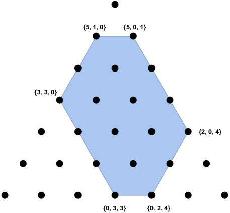
Figure 1. Zonotopal generalized permutohedron for Example 13, $(c_{12},c_{23},c_{13})=(2,1,3)$. All edges parallel to $e_{i}-e_{j}$ have length $c_{ij}$.

Example 13.

Consider the case $\mathcal{K}^{3}$. Let the matrix of constants $\mathcal{D}$ be given, with nonzero entries $c_{12}=c_{21}=2,\ c_{23}=c_{32}=1,\ c_{13}=c_{31}=3$. The characteristic function of the zonotopal generalized permutohedron in Figure 1 has the following expansion:

$$[[12_{2}]]\bullet[[23_{1}]]\bullet[[13_{3}]]$$

$$=[[1,2,3]]_{\mathcal{D}}+[[2,1,3]]_{\mathcal{D}}+[[2,3,1]]_{\mathcal{D}}+[[3,2,1]]_{\mathcal{D}}+[[3,1,2]]_{\mathcal{D}}+[[1,3,2]]_{\mathcal{D}}$$

$$-\left([[1,23]]_{\mathcal{D}}+[[12,3]]_{\mathcal{D}}+[[2,13]]_{\mathcal{D}}+[[23,1]]_{\mathcal{D}}+[[3,12]]_{\mathcal{D}}+[[13,2]]_{\mathcal{D}}\right)$$

$$+[[123]]_{\mathcal{D}}$$

$$=[[1_{0}2_{2}3_{4}]]+[[2_{0}1_{2}3_{4}]]+[[2_{0}3_{1}1_{5}]]+[[3_{0}2_{1}1_{5}]]+[[3_{0}1_{3}2_{3}]]+[[1_{0}3_{3}2_{3}]]$$

$$-\left([[1_{0}23_{6}]]+[[12_{2}3_{4}]]+[[2_{0}13_{6}]]+[[23_{1}1_{5}]]+[[3_{0}12_{6}]]+[[13_{3}2_{3}]]\right)$$

$$+[[123_{6}]],$$

where for example $[[1_{0}2_{2}3_{4}]]$ is the characteristic function of the cone at the vertex $(0,2,4)$ opening toward the upper left, cut out by the inequalities

$$x_{1} \geq 0$$

$$x_{12} \geq 0+2$$

$$x_{123} = 0+2+4.$$

The corresponding sum of fractions from (1) in terms of generalized Mandelstam variables $s_{J}$ is

$$\frac{1}{s_{a1}s_{a12}}+\frac{1}{s_{a1}s_{a13}}+\frac{1}{s_{a2}s_{a21}}+\frac{1}{s_{a2}s_{a23}}+\frac{1}{s_{a3}s_{a31}}+\frac{1}{s_{a3}s_{a32}}$$

$$=\frac{1}{(x_{1})(x_{12}-2)}+\frac{1}{(x_{1})(x_{13}-3)}+\frac{1}{(x_{2})(x_{21}-2)}+\frac{1}{(x_{2})(x_{23}-1)}+\frac{1}{(x_{3})(x_{31}-3)}+\frac{1}{(x_{3})(x_{32}-1)},$$

where we recall that $x_{ij}=x_{i}+x_{j}$.

Example 14.

See Figure 2 for the explosion of a point to a hexagon, as the Minkowski sums $[12_{\varepsilon}]+[13_{\varepsilon}]+[23_{\varepsilon}]=\left\{u_{12}+u_{13}+u_{23}:u_{ij}\in[ij_{\varepsilon}]\right\}$ from Theorem 8 for (small) $\varepsilon\geq 0$.

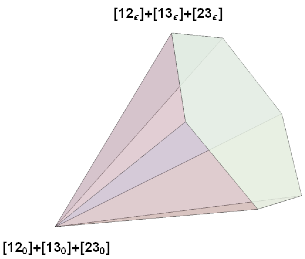
Figure 2. Exploding a point to a hexagon: $(c_{12},c_{13},c_{23})=(\varepsilon,\varepsilon,\varepsilon)$ for $\varepsilon\geq 0$

When $\varepsilon>0$ the expression does not have a canonical simplification,

$$\frac{1}{x_{2}\left(x_{1}+x_{2}-\epsilon\right)}+\frac{1}{x_{1}\left(x_{1}+x_{3}-\epsilon\right)}+\frac{1}{x_{3}\left(x_{1}+x_{3}-\epsilon\right)}+\frac{1}{x_{2}\left(x_{2}+x_{3}-\epsilon\right)}+\frac{1}{x_{3}\left(x_{2}+x_{3}-\epsilon\right)}+\frac{1}{x_{1}\left(x_{1}+x_{2}-\epsilon\right)},$$

but in the limit $\varepsilon\rightarrow 0$ we have

$$\frac{1}{x_{2}\left(x_{1}+x_{2}\right)}+\frac{1}{x_{1}\left(x_{1}+x_{3}\right)}+\frac{1}{x_{3}\left(x_{1}+x_{3}\right)}+\frac{1}{x_{2}\left(x_{2}+x_{3}\right)}+\frac{1}{x_{3}\left(x_{2}+x_{3}\right)}+\frac{1}{x_{1}\left(x_{1}+x_{2}\right)}=\frac{x_{1}+x_{2}+x_{3}}{x_{1}x_{2}x_{3}}=0,$$

since the numerator vanishes identically. This can also be seen from general theory, as higher codimension cones (in particular, here, the point at the origin) are in the kernel of the valuation induced by the integral Laplace transform.

3. Generalized associahedra in the kinematic space

The standard realization of the associahedron was given, see [13], in terms of facet inequalities, as

$$\left\{x\in\mathbb{R}^{n}:\ \sum_{i=1}^{n}x_{i}=\binom{n}{2},\ \sum_{i\in I}x_{i}\geq\binom{|I|+1}{2}:I=[a,b]\subsetneq\{1,\ldots,n\}\right\},$$

where $[a,b]$ runs over all proper subintervals of $\{1,\ldots,m\}$ with $b-a\geq 2$.

Having a binomial coefficients for the vertex coordinates begs the question whether they are counting some quantity. We show in what follows that they are counting the Mandelstam parameters $s_{ij}$ for all $i\not\in\{j-1,j,j+1\}$, specialized to the hyperplane where $s_{ij}=-c_{ij}=-1$.

The following construction in the kinematic for an arbitrary graph appeared first in [12], where the resulting generalized permutohedron is called a Cayley polytope.

Let a collection of constants

$$\mathcal{D}=\{c_{ij}=c_{ji}\geq 0:1\leq i,j\leq n+1,\ i\not\in\{j-1,j,j+1\}\}$$

be given. Define

$$\mathcal{A}^{n}(\mathcal{D})=\left\{(s)\in\mathcal{K}^{n}:\ s_{ij}=-c_{ij}\text{ whenever }i\not\in\{j-1,j,j+1\};\ s_{[a,b]}\geq 0,\ i,j,a,b=1,\ldots,n+1\right\},$$

where we use the notation $[a,b]=\{a,a+1,\ldots,b\}$.

Proposition 15.

The set $\mathcal{A}^{n}(\mathcal{D})$ is a generalized permutohedron, and can be expressed as a Minkowski sum, as

$$\{[(i\ i+1\cdots j-1\ j)_{c_{i,j+1}}]:1\leq i<j\leq n\},$$

where $[(i\ i+1\cdots j-1\ j)_{c_{i,j+1}}]$ is the dilated simplex which is given by the convex hull of the set of vertices $\{c_{i,j+1}e_{i},c_{i,j+1}e_{i+1},\ldots,c_{i,j+1}e_{j-1},c_{i,j+1}e_{j}\}$. In the case when all constants $c_{i,j+1}$ tend to $1$, then we recover exactly the usual associahedron.

Sketch of proof.

This follows from Proposition 7.5 in [18], where the dilation parameter $y_{J}$ for each contiguous subset $\{i,i+1,\ldots,j\}$ is now $c_{i,j+1}$, and where $y_{J}=0$ for all non-contiguous subsets $J\subset\{1,\ldots,m\}$. ∎

It is easy to check verify from the definition of $\mathcal{A}^{n}$, using the property $s_{I}=s_{I^{c}}$ for $I\subsetneq$ a nonempty subset of $\{1,\ldots,n+2\}$, that the kinematic space has a natural action of $\mathbb{Z}/(n+2)\mathbb{Z}$ which preserves the set of equations which cut out the $(n-1)$-dimensional associahedron.

Indeed, then the pointwise action on the associahedron by $\sigma=(12\cdots n)$ becomes

$$(s_{12},s_{23},\ldots,s_{n-2,n-1})\mapsto(s_{23},s_{34},\ldots,s_{n-1,n})=(s_{23},s_{34},\ldots,s_{n-2,n-1},s_{12\cdots n-2})$$

$$= \left(s_{23},s_{34},\ldots,s_{n-2,n-1},\sum_{i=1}^{n-2}s_{i,i+1}-\sum_{1\leq i<j-1\leq n-3}c_{ij}\right),$$

where the sum is over the constants $s_{i,j}=-c_{i,j}$ having nonadjacent indices $i<j-1\leq n-3$.

This gives rise to Proposition 16.

Proposition 16.

The action of the $(n+2)$-cycle $\sigma=(12\cdots(n+2))$ on the kinematic space $\mathcal{K}^{n}$ preserves the natural embedding of the $(n-1)$-dimensional associahedron.

Example 17.

In the case $m=5$ we have variables $(x_{1},x_{2},x_{3})=(s_{12},s_{23},s_{34})$, where $x_{1}+x_{2}+x_{3}$ will be constant. In terms of the Mandelstam variables, the 2-dimensional associahedron is cut out by the inequalities

$$s_{12},s_{23},s_{34},s_{123},s_{234}\geq 0.$$

The inequalities defining the tangent cones at the five vertices are labeled by nesting intervals, as

$$(s_{12},s_{123}\geq 0,\ \ s_{23},s_{123}\geq 0,\ \ s_{23},s_{234}\geq 0,\ \ s_{34},s_{234}\geq 0,\ \ s_{12},s_{34}\geq 0).$$

These map termwise under $\sigma=(12345)$ to

$$(s_{23},s_{234}\geq 0,\ \ s_{34},s_{234}\geq 0,\ \ s_{34},s_{12}\geq 0,\ \ s_{123},s_{12}\geq 0,\ \ s_{23},s_{123}\geq 0),$$

having used the relations $s_{345}=s_{12}$ and $s_{45}=s_{123}$ to remove the index $5$. Then, in the $x$-coordinates this becomes

$$x_{1} \geq 0$$

$$x_{2} \geq 0$$

$$x_{3} \geq 0$$

$$x_{1}+x_{2} \geq c_{13}$$

$$x_{2}+x_{3} \geq c_{24}$$

$$x_{1}+x_{2}+x_{3} = c_{13}+c_{24}+c_{14},$$

where the last line holds identically in the kinematic space. The vertices are given by

$$\{(0,c_{13},c_{24}+c_{14}),(0,c_{13}+c_{24}+c_{14},0),(c_{13},0,c_{24}+c_{14}),(c_{13}+c_{14},0,c_{24}),(c_{13}+c_{14},c_{24},0)\}.$$

This is the Minkowski sum of a triangle of edge length 3, and two line segments. In terms of characteristic functions, using the convolution product we have

$$[[123_{c_{14}}]]\bullet[[12_{c_{13}}]]\bullet[[23_{c_{24}}],$$

where the triangle and two lines are given by

$$[[123_{c_{14}}]]=\left\{x\in[0,c_{14}]^{3}:\sum_{i=1}^{3}x_{i}=c_{14}\right\},$$

$$[[12_{c_{13}}]]=\left\{x\in[0,c_{13}]^{3}:\sum_{i=1}^{3}x_{i}=c_{13},\ x_{3}=0\right\},$$

$$[[23_{c_{24}}]]=\left\{x\in[0,c_{24}]^{3}:\sum_{i=1}^{3}x_{i}=c_{24},\ x_{1}=0\right\}.$$

In the case that $(c_{13},c_{24},c_{14})=(1,1,1)$ we recover the usual associahedron, as a generalized permutohedron, see Figure 3.

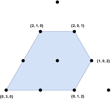
Figure 3.

For the case that $(c_{13},c_{24},c_{14})=(2,1,3)$ see see Figure 4.

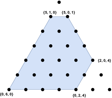
Figure 4.

4. Triangulations of permutohedral cones and the associahedron

Let us fix $m=n+1$.

We here illustrate the tree triangulation of the plate $[1,2,\ldots,m]$, which we recall from [7] can be expressed as the conical hull

$$[1,2,\ldots,m]=\langle e_{1}-e_{2},\ldots,e_{m-1}-e_{m}\rangle_{+}:=\left\{t_{1}(e_{1}-e_{2})+\cdots+t_{m-1}(e_{m-1}-e_{m}):t_{i}\geq 0\right\}.$$

Fix an order $(1,\ldots,m)$ for $m$ vertices on the line. Following [10], we see that the set of (unlayered) binary trees growing up from a given root, having $1,\ldots,m$ as leaves, are in an obvious bijection with directed trees with edges

$$\left\{(i_{1},j_{1}),\ldots,(i_{m-2},j_{m-2}),(1,m)\right\},$$

such that the intervals $\{i_{a},i_{a}+1,\ldots,j_{a}\}$ are either nested or disjoint, and where $(1,m)$ is always an edge. See Figure 5 for the case $m=4$.

Definition 18.

Denote by $\text{Trees}^{m}$ the set of all such trees with leaves in the order $(1,\ldots,m)$. Call a partial tree a directed graph which is obtained by removing a subset of the edges

$$\{(i_{1},j_{1}),\ldots,(i_{m-2},j_{m-2})\}$$

from a tree $\{(i_{1},j_{1}),\ldots,(i_{m-2},j_{m-2}),(1,m)\}\in\text{Trees}^{m}$. Denote by $\text{Tree}_{\leq}^{n}$ the set of all partial trees.

Proposition 19.

The set of simplicial cones

$$\left\{\langle(i_{1},j_{1}),\ldots,(i_{m-2},j_{m-2}),(1,m)\rangle_{+}:\{(i_{1},j_{1}),\ldots,(i_{m-2},j_{m-2}),(1,m)\}\in\text{Trees}^{m}\right\}$$

decomposes $\langle e_{1}-e_{2},\ldots,e_{m-1}-e_{m}\rangle_{+}$ into $C_{m-1}=\frac{1}{m}\binom{2(m-1)}{m-1}$ simplicial cones which have disjoint interiors, where $C_{a}$ is the $a^{\text{th}}$ Catalan number.

Proof.

This follows by a slight extension of Theorem 6.3 in [10], replacing the convex hull of the positive roots with their conical hull

$$\langle\{e_{i}-e_{j}:1\leq i<j\leq m\}\rangle_{+}=\langle e_{1}-e_{2},\ldots,e_{m-1}-e_{m}\rangle_{+}=[1,2,\ldots,m].$$

∎

Example 20.

With $m=4$ we have the set-theoretic union

$$\langle e_{1}-e_{2},e_{2}-e_{3}\rangle_{+}=\langle e_{1}-e_{3},e_{2}-e_{3}\rangle_{+}\cup\langle e_{1}-e_{2},e_{1}-e_{3}\rangle_{+}.$$

Note that this provides a nice interpretation of the fundamental rational function identity

$$\frac{1}{(y_{1}-y_{2})(y_{2}-y_{3})}=\frac{1}{(y_{1}-y_{3})(y_{2}-y_{3})}+\frac{1}{(y_{1}-y_{2})(y_{1}-y_{3})},$$

where the common boundary line has been ignored.

Then, there is a natural duality between the plate $[1,2,\ldots,m]$ and the $(m-2)$-dimensional associahedron.

Proposition 21.

The face poset of the set of simplicial cones in the tree triangulation of the standard plate $\pi_{0}=\langle e_{1}-e_{2},\ldots,e_{m-1}-e_{m}\rangle+$ is in duality with the set of tangent cones to the associahedron.

Proof.

Let us fix $s_{ij}=-c_{ij}=-1$ for all nonadjacent indices $i<j-1$, for $1\leq i,j\leq m$. Collect these values of the $c_{ij}$ in the matrix $\mathcal{D}$, as usual.

To the face given by the conical hull $\langle e_{i_{1}}-e_{j_{1}},\ldots,e_{i_{a}}-e_{j_{a}}\rangle_{+}$ of the tree triangulation of $\pi_{0}$ encoded by the partial tree $\{(i_{1},j_{1}),\ldots,(i_{a},j_{a})\}\in\text{Tree}_{\leq}^{m}$, where $1\leq a\leq m-1,$ we assign the tangent cone to the face of the associahedron:

$$\langle e_{i_{1}}-e_{j_{1}},\ldots,e_{i_{a}}-e_{j_{a}}\rangle_{+}\mapsto\{s\in\mathcal{K}^{m}(\mathcal{D}):s_{i_{1}\cdots j_{1}+1}\geq 0,\ldots,s_{i_{a}\cdots j_{a}+1}\geq 0\}.$$

For the converse, note that the elements $\{(i_{1},j_{1}),\ldots,(i_{m-1}-j_{m-1})\}\in\text{Tree}^{m}$ label the (top-dimensional) simplicial cones in the triangulation, and that these are in duality with exactly the tangent cones to the vertices of the associahedron, according to the correspondence above. It is easy to see from the construction that this correspondence reverses inclusion of sets. Indeed, any face of the triangulation is obtained by removing 1 or more generators $\{e_{i_{\alpha}}-e_{j_{\alpha}}:\alpha\in A\}$ from some simplicial cone, and conversely the tangent cone to any face of the associahedron is obtained by removing 1 or more inequalities

$$\{s_{i_{\alpha}\cdots s_{j_{\alpha}}}\geq 0:\alpha\in A\}.$$

This completes the proof.

∎

Recall the following formula for the Laplace transform: if $\pi=\langle e_{i_{1}}-e_{j_{1}},\ldots,e_{i_{m-1}}-e_{j_{m}}\rangle_{+}$ is a (simplicial) cone, then the Laplace transform of $\pi$ is given by

$$\int_{u\in\pi}e^{-u\cdot\mathbf{y}}du=\int_{t_{i}\geq 0}e^{-t_{1}(y_{i_{1}}-y_{j_{1}})-\cdots-t_{m-1}(y_{i_{m-1}}-y_{j_{m-1}})}=\frac{1}{(y_{i_{1}}-y_{j_{1}})\cdots(y_{i_{m-1}}-y_{j_{m-1}})}.$$

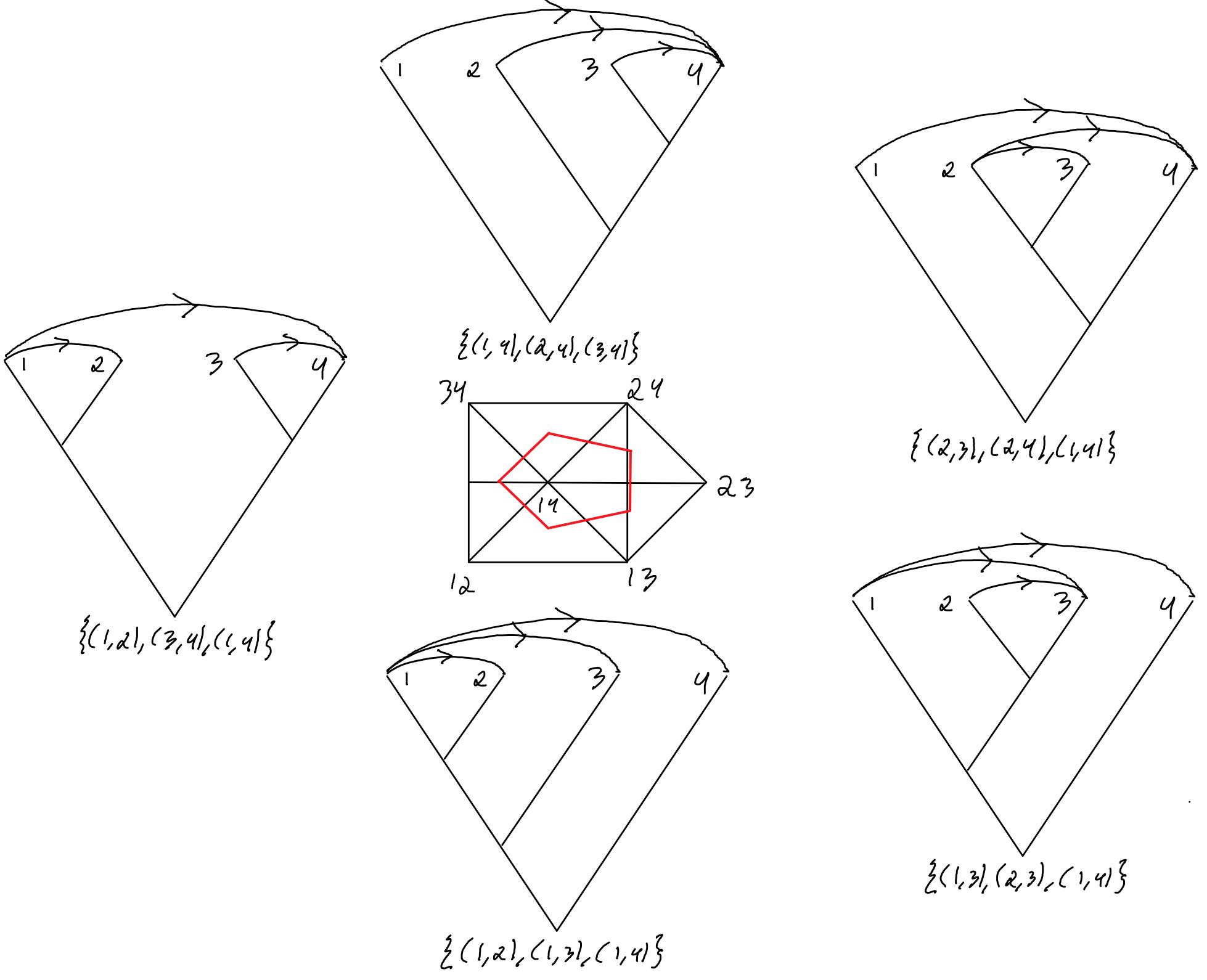
Figure 5. Top-dimensional simplicial cones in the triangulation of the standard plate $[1,2,3,4]$ are dual to tangent cones to vertices of the associahedron (outlined schematically in red). See Example 22.

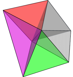
Figure 6. See Example 22; triangulation of the root cone $\langle e_{1}-e_{2},e_{2}-e_{3},e_{3}-e_{4}\rangle_{+}.$

Example 22.

Set $h_{ij}=e_{i}-e_{j}$. We consider the case $m=5$.

The triangulation of $[1,2,3,4]=\langle h_{12},h_{23},h_{34}\rangle_{+}$ is represented by the sum of the Laplace transforms of its five simplicial cones,

$$\langle h_{12},h_{13},h_{14}\rangle_{+},\langle h_{13},h_{23},h_{14}\rangle_{+},\langle h_{12},h_{34},h_{14}\rangle_{+},\langle h_{14},h_{23},h_{24}\rangle_{+},\langle h_{14},h_{24},h_{34}\rangle_{+},$$

as

$$\frac{1}{\left(y_{1}-y_{2}\right)\left(y_{2}-y_{3}\right)\left(y_{3}-y_{4}\right)}$$

$$=\frac{1}{\left(y_{1}-y_{2}\right)\left(y_{1}-y_{3}\right)\left(y_{1}-y_{4}\right)}+\frac{1}{\left(y_{1}-y_{3}\right)\left(y_{2}-y_{3}\right)\left(y_{1}-y_{4}\right)}+\frac{1}{\left(y_{1}-y_{2}\right)\left(y_{1}-y_{4}\right)\left(y_{3}-y_{4}\right)}$$

$$+\frac{1}{\left(y_{2}-y_{3}\right)\left(y_{1}-y_{4}\right)\left(y_{2}-y_{4}\right)}+\frac{1}{\left(y_{1}-y_{4}\right)\left(y_{2}-y_{4}\right)\left(y_{3}-y_{4}\right)},$$

see Figures 5 and 6. Note that here we have neglected characteristic functions of common faces. Indeed, we have the identity of characteristic functions, modulo characteristic functions of faces,

$$[[1,2]]\bullet[[2,3]]\bullet[[3,4]]$$

$$= [[1,3]]\bullet[[2,3]]\bullet[[1,4]]+[[2,3]]\bullet[[1,4]]\bullet[[2,4]]$$

$$+ [[1,2]]\bullet[[1,4]]\bullet[[3,4]]+[[1,4]]\bullet[[2,4]]\bullet[[3,4]]+[[1,2]]\bullet[[1,3]]\bullet[[1,4]],$$

where $[[i,j]]\bullet[[k,\ell]]$ equals the characteristic function of the conical hull $\langle e_{i}-e_{j},e_{k}-e_{\ell}\rangle_{+}$, in the notation from [7].

Recall that the integral Laplace transform has in its kernel the span of all characteristic functions of higher codimension faces, as well as the characteristic function of any non-pointed cone (i.e. a cone which contains a double infinite line, such as the whole space). For example, this gives a polytopal explanation for why the cyclic sum vanishes:

$$\frac{1}{(y_{1}-y_{2})\cdots(y_{m-1}-y_{m})}+\frac{1}{(y_{2}-y_{3})\cdots(y_{m}-y_{1})}+\cdots+\frac{1}{(y_{m}-y_{1})\cdots(y_{m-1}-y_{m})}=0,$$

that is, because it can be shown that the $n$ cyclically rotated simplicial cones $[1,2,\ldots,n]$ have union the whole space and have non-intersecting interiors.

On the other hand, while characteristic functions of non-pointed cones are in the kernel of the functional representation $[[i,j]]\mapsto\sum_{a=0}^{\infty}e^{-(y_{i}-y_{j})}=\frac{1}{1-x_{i}/x_{j}}$, where $x_{i}=e^{-y_{i}}$, the higher codimension faces are not. See for example [3] for details about functional representations of polyhedral cones. In the case at hand, corresponding to the present triangulation we have the functional identity

$$\frac{1}{\left(1-\frac{x_{1}}{x_{3}}\right)\left(1-\frac{x_{2}}{x_{3}}\right)\left(1-\frac{x_{1}}{x_{4}}\right)}+\frac{1}{\left(1-\frac{x_{2}}{x_{3}}\right)\left(1-\frac{x_{1}}{x_{4}}\right)\left(1-\frac{x_{2}}{x_{4}}\right)}+\frac{1}{\left(1-\frac{x_{1}}{x_{2}}\right)\left(1-\frac{x_{1}}{x_{3}}\right)\left(1-\frac{x_{1}}{x_{4}}\right)}$$

$$+ \frac{1}{\left(1-\frac{x_{1}}{x_{2}}\right)\left(1-\frac{x_{1}}{x_{4}}\right)\left(1-\frac{x_{3}}{x_{4}}\right)}+\frac{1}{\left(1-\frac{x_{1}}{x_{4}}\right)\left(1-\frac{x_{2}}{x_{4}}\right)\left(1-\frac{x_{3}}{x_{4}}\right)}$$

$$- \left(\frac{1}{\left(1-\frac{x_{1}}{x_{3}}\right)\left(1-\frac{x_{1}}{x_{4}}\right)}+\frac{1}{\left(1-\frac{x_{2}}{x_{3}}\right)\left(1-\frac{x_{1}}{x_{4}}\right)}+\frac{1}{\left(1-\frac{x_{1}}{x_{4}}\right)\left(1-\frac{x_{2}}{x_{4}}\right)}+\frac{1}{\left(1-\frac{x_{1}}{x_{4}}\right)\left(1-\frac{x_{3}}{x_{4}}\right)}\right.$$

$$+ \left.\frac{1}{\left(1-\frac{x_{1}}{x_{2}}\right)\left(1-\frac{x_{1}}{x_{4}}\right)}\right)+\frac{1}{1-x_{1}/x_{4}}$$

$$= \frac{1}{\left(1-\frac{x_{1}}{x_{2}}\right)\left(1-\frac{x_{2}}{x_{3}}\right)\left(1-\frac{x_{3}}{x_{4}}\right)},$$

which is the Laplace transform of the standard plate $[1,2,3,4]$. Here the subtracted fractions are discrete Laplace transforms of the 2-dimensional simplicial cones respectively

$$\langle h_{13},h_{14}\rangle_{+},\langle h_{23},h_{14}\rangle_{+},\langle h_{14},h_{24}\rangle_{+},\langle h_{14},h_{34}\rangle_{+},\langle h_{12},h_{14}\rangle_{+},$$

and the fraction in the last line is identified with the central ray $\langle h_{14}\rangle_{+}$, seen in Figures 5 and 6 as the central vertex labeled $14$, which is shorthand for $\langle e_{1}-e_{4}\rangle_{+}$.

Let us make a comparison between the expression above and the formula in Section 4.3 of [15] for the generic diagonal element of the KLT matrix:

$$\langle C(12345),C(12345)\rangle = 1-\left(\frac{1}{1-e^{2\pi is_{12}}}+\frac{1}{1-e^{2\pi is_{23}}}+\frac{1}{1-e^{2\pi is_{34}}}+\frac{1}{1-e^{2\pi is_{45}}}+\frac{1}{1-e^{2\pi is_{51}}}\right)$$

$$+ \frac{1}{(1-e^{2\pi is_{12}})(1-e^{2\pi is_{34}})}+\frac{1}{(1-e^{2\pi is_{23}})(1-e^{2\pi is_{45}})}$$

$$+ \frac{1}{(1-e^{2\pi is_{34}})(1-e^{2\pi is_{51}})}+\frac{1}{(1-e^{2\pi is_{45}})(1-e^{2\pi is_{12}})}$$

$$+ \frac{1}{(1-e^{2\pi is_{51}})(1-e^{2\pi is_{23}})}.$$

See also [9] for an inclusion/exclusion derivation of terms in the diagonal of the inverse KLT matrix.

We construct an explicit identification, using the identity $s_{45}=s_{123}$ and its permutations to eliminate the label $5$. This gives

$$\langle C(12345),C(12345)\rangle = 1-\left(\frac{1}{1-e^{2\pi is_{12}}}+\frac{1}{1-e^{2\pi is_{23}}}+\frac{1}{1-e^{2\pi is_{34}}}+\frac{1}{1-e^{2\pi is_{123}}}+\frac{1}{1-e^{2\pi is_{234}}}\right)$$

$$+ \frac{1}{(1-e^{2\pi is_{12}})(1-e^{2\pi is_{34}})}+\frac{1}{(1-e^{2\pi is_{23}})(1-e^{2\pi is_{123}})}$$

$$+ \frac{1}{(1-e^{2\pi is_{34}})(1-e^{2\pi is_{234}})}+\frac{1}{(1-e^{2\pi is_{123}})(1-e^{2\pi is_{12}})}$$

$$+ \frac{1}{(1-e^{2\pi is_{234}})(1-e^{2\pi is_{23}})}.$$

The termwise identification here is as follows:

$$1\Leftrightarrow\frac{1}{1-x_{1}/x_{4}}\ \ \ \ \ \ \ \ \ \ \ \ \$$

$$\frac{1}{1-e^{2\pi is_{12}}}\Leftrightarrow\frac{1}{1-x_{1}/x_{2}}\frac{1}{1-x_{1}/x_{4}} \frac{1}{1-e^{2\pi is_{12}}}\frac{1}{1-e^{2\pi is_{34}}}\Leftrightarrow\frac{1}{(1-x_{1}/x_{2})(1-x_{3}/x_{4})(1-x_{1}/x_{4})}$$

$$\frac{1}{1-e^{2\pi is_{23}}}\Leftrightarrow\frac{1}{1-x_{2}/x_{3}}\frac{1}{1-x_{1}/x_{4}} \frac{1}{1-e^{2\pi is_{23}}}\frac{1}{1-e^{2\pi is_{123}}}\Leftrightarrow\frac{1}{(1-x_{2}/x_{3})(1-x_{1}/x_{3})(1-x_{1}/x_{4})}$$

$$\frac{1}{1-e^{2\pi is_{34}}}\Leftrightarrow\frac{1}{1-x_{3}/x_{4}}\frac{1}{1-x_{1}/x_{4}} \frac{1}{1-e^{2\pi is_{34}}}\frac{1}{1-e^{2\pi is_{234}}}\Leftrightarrow\frac{1}{(1-x_{3}/x_{4})(1-x_{2}/x_{4})(1-x_{1}/x_{4})}$$

$$\frac{1}{1-e^{2\pi is_{123}}}\Leftrightarrow\frac{1}{1-x_{1}/x_{3}}\frac{1}{1-x_{1}/x_{4}} \frac{1}{1-e^{2\pi is_{123}}}\frac{1}{1-e^{2\pi is_{12}}}\Leftrightarrow\frac{1}{(1-x_{1}/x_{3})(1-x_{1}/x_{2})(1-x_{1}/x_{4})}$$

$$\frac{1}{1-e^{2\pi is_{234}}}\Leftrightarrow\frac{1}{1-x_{2}/x_{4}}\frac{1}{1-x_{1}/x_{4}} \frac{1}{1-e^{2\pi is_{234}}}\frac{1}{1-e^{2\pi is_{23}}}\Leftrightarrow\frac{1}{(1-x_{2}/x_{4})(1-x_{2}/x_{3})(1-x_{1}/x_{4})}$$

Remark 23.

Dualizing term-by-term the formula given in Lemma 4.1 in [15] for the self-intersection number,

$$\langle C(1,2,\ldots,m),C(1,2,\ldots,m)\rangle=\sum_{k=0}^{m-2}\sum_{F=H_{1}\cap\cdots\cap H_{k}}(-1)^{m-2-k}\frac{1}{(1-e^{2\pi i{H_{1}}})\cdots(1-e^{2\pi i{H_{k}}})},$$

then we obtain exactly the general formula for the expansion as a signed sum of fractions. Indeed, we have the alternating sum over the faces of the triangulation of

$$\langle e_{1}-e_{2},\ldots,e_{m-1}-e_{m}\rangle_{+},$$

$$\frac{1}{(1-x_{1}/x_{2})\cdots(1-x_{m-1}/x_{m})}=\sum_{k=1}^{m-1}(-1)^{m-1-k}\sum_{\{(i_{1},j_{1}),\ldots,(i_{k},j_{k}),(1,m)\}}\frac{1}{(1-x_{i_{1}}/x_{j_{1}})\cdots(1-x_{i_{k}}/x_{j_{k}})},$$

labeled by the set of partial trees $\text{Tree}_{\leq}^{M}$.

In Section 5 we formalize the above discussion.

5. Restricting $m$ and $m_{\alpha^{\prime}}$ to the nearest-neighbor subspace of the kinematic space

Denote by $X^{n}$ the subspace of all symmetric (real) $n\times n$ matrices with

1. $s_{ii}=0$ for $i=1,\ldots,n-1$.

2. $s_{ij}=0$ whenever $|i-j|>1$, for $1\leq i,j\leq n-1$ (“nearest neighbor” interactions only).

3. $s_{in}=-\sum_{j=1}^{n-1}s_{ij}$ for each $i=1,\ldots,n-1$.

4. $s_{nn}=\sum_{1\leq i<j\leq n-1}s_{ij}$ $(=s_{12\cdots n-1})$ (“massive $n^{\text{th}}$ particle”).

For example, a generic element of $X^{6}$ looks like

$$\begin{bmatrix}0&s_{12}&0&0&0&-s_{12}\\ s_{12}&0&s_{23}&0&0&-(s_{12}+s_{23})\\ 0&s_{23}&0&s_{34}&0&-(s_{23}+s_{34})\\ 0&0&s_{34}&0&s_{45}&-(s_{34}+s_{45})\\ 0&0&0&s_{45}&0&-s_{45}\\ -s_{12}&-(s_{12}+s_{23})&-(s_{23}+s_{34})&-(s_{34}+s_{45})&-s_{45}&\sum_{i=1}^{4}s_{i,i+1}\end{bmatrix}$$

Our main result is to prove the following identities for the biadjoint amplitude and its $\alpha^{\prime}$ deformation; notation will be explained subsequently.

Theorem 24.

On the support of $X^{n}$, $m$ and $m_{\alpha^{\prime}}$ simplify to respectively

$$m(PT(1,\ldots,n),PT(1,\ldots,n))\big{|}_{X^{n}} = \frac{s_{12\cdots n-1}}{s_{12}s_{23}\cdots s_{n-2,n-1}}$$

$$m_{\alpha^{\prime}}(PT(1,\ldots,n),PT(1,\ldots,n))\big{|}_{X^{n}} = \frac{1-\exp\left(-2\pi i\alpha^{\prime}\sum_{i=1}^{n-2}s_{i,i+1}\right)}{\prod_{i=1}^{n-2}\left(1-e^{-2\pi i\alpha^{\prime}s_{i,i+1}}\right)}.$$

The proof will involve the following change of variable, to transform the computation into an application of inclusion exclusion for simplicial cones: gathering together the independent coordinates of any $(s)\in X^{n}$ in an $(n-2)$-tuple $(s_{12},s_{23},\ldots,s_{n-2,n-1})$, let $(y_{1},\ldots,y_{n})\in\mathbb{R}^{n}$ such that $s_{i,i+1}=y_{i}-y_{i+1}$ for each $i=1,\ldots,n-2$. Note that $(y_{1},\ldots,y_{n})$ is defined up to translation by a multiple of $(1,1,\ldots,1)$.

Remark 25.

It is interesting to note that the biadjoint amplitude is proportional the mass of the $n^{\text{th}}$ particle, since by momentum conservation we have $s_{12\cdots n-1}=\left(\sum_{i=1}^{n-1}p_{i}\right)^{2}=p_{n}^{2}$. Moreover, for the regular biadjoint amplitude, since

$$s_{12\cdots n-1}=s_{12}+s_{23}+\cdots+s_{n-2,n-1}$$

we have the intriguing simplification

$$m(PT(1,\ldots,n),PT(1,\ldots,n))\big{|}_{X^{n}}=\sum_{i=1}^{n-2}\frac{1}{s_{12}s_{23}\cdots\widehat{s_{i,i+1}}\cdots s_{n-2,n-1}},$$

where the terms in the summation are in bijection with the $(n-2)$ boundary facets of the polyhedral cone

$$\langle e_{1}-e_{2},e_{2}-e_{3},\ldots,e_{n-2}-e_{n-1}\rangle_{+}=\left\{\sum_{i=1}^{n-2}t_{i}(e_{i}-e_{i+1}):t_{i}\geq 0\right\}$$

from above, see Figures 5 and 6.

Taking into account the change of variable, the first identity in Theorem 24 becomes

$$m(PT(1,\ldots,n),PT(1,\ldots,n))\big{|}_{X^{n}} = \mathcal{L}_{\int}(\langle e_{1}-e_{2},\ldots,e_{n-2}-e_{n-1}\rangle_{+})\cdot(y_{1}-y_{n-1})$$

$$= \sum_{i=1}^{n-2}\mathcal{L}_{\int}(\langle e_{1}-e_{2},\ldots,\widehat{e_{i}-e_{i+1}},\ldots,e_{n-2}-e_{n-1}\rangle_{+}),$$

the sum of the integral Laplace transforms over the boundary components of the cone

$$\langle e_{1}-e_{2},\ldots,e_{n-2}-e_{n-1}\rangle_{+}=\{t_{1}(e_{1}-e_{2})+\cdots+t_{n-1}(e_{n-2}-e_{n-1}):t_{i}\geq 0\},$$

where for the integrals the measure is taken on the respective ambient subspace.

Now let $\partial^{k}(\pi_{\sigma})$ denote the set of faces of dimension $k$.

Then we have

$$m_{\alpha^{\prime}}(PT(1,\ldots,n),PT(1,\ldots,n))\big{|}_{X^{n}}=\mathcal{L}_{\sum}(\langle e_{1}-e_{2},\ldots,e_{n-2}-e_{n-1}\rangle_{+})\cdot(1-e^{-(y_{1}-y_{n-1})})$$

$$= \sum_{J\subsetneq\{1,2,\ldots,n-1\}}(-1)^{(n-2)-|J|}\mathcal{L}_{\sum}\left(\left\langle\{e_{j}-e_{j+1}:j\in J\}\right\rangle\right),$$

which is an application of inclusion/exclusion to the set of all faces of codimension at least $1$ the cone

$$\langle e_{1}-e_{2},\ldots,e_{n-2}-e_{n-1}\rangle_{+}.$$

Let $\mathcal{T}_{n}$ be the set of all (partial) triangulations of a polygon $\text{poly}_{n}$ oriented counterclockwise with vertices $1,2,\ldots,n$; these partial triangulations are in correspondence with faces of the associahedron, or dually with the faces of the simplicial complex formed from the standard triangulation of the simplicial cone

$$\langle e_{1}-e_{2},\ldots,e_{n-2}-e_{n-1}\rangle_{+}.$$

This can be seen by taking the cone over the triangulation of the so-called root polytope from [10], see also [6] for a proof of the triangulation by adding relative volumes of simplices.

For example, the set of forests each having a single tree consists of the $C_{n}$ binary trees, where $C_{n}=\frac{1}{n-1}\binom{2(n-2)}{2}$ is the Catalan number; these label the maximal dimension simplicial cones in the triangulation.

Let us express the formula for $\langle C(1,2,\ldots,n),C(1,2,\ldots,n)\rangle$ from [15] in terms of partial triangulations. We recall that

(6) $$\langle C(1,2,\ldots,n),C(1,2,\ldots,n)\rangle=\sum_{T\in\mathcal{T}_{n}}(-1)^{(n-3)-|T|}\prod_{E\in T}\frac{1}{1-e^{-2\pi i\alpha^{\prime}s_{\overline{E}}}}$$

as $T$ ranges over all partial triangulations of $\text{poly}_{n}$ and $E\in T$ ranges over the edges of $T$, and where $|T|$ is the number of edges $E$ of $T$. Here $s_{\overline{E}}=s_{ii+1\cdots j}$ if $E=(i,j)$.

We observe that the restriction of the right-hand side of Equation (6) to $X^{n}$ gives rise to a termwise identification with the sums of the Laplace transforms of the boundary components of the cone

$$\langle e_{1}-e_{2},\ldots,e_{n-2}-e_{n-1}\rangle_{+}=\{t_{1}(e_{1}-e_{2})+\cdots+t_{n-1}(e_{n-2}-e_{n-1}):t_{i}\geq 0\}.$$

Given an n-cycle $\sigma=(\sigma_{1},\sigma_{2},\ldots,\sigma_{n})$ with minimal element $\sigma_{1}$, let use define $\pi_{\sigma}=\langle e_{\sigma_{1}}-e_{\sigma_{2}},\ldots,e_{\sigma_{n-1}}-e_{\sigma_{n}}\rangle_{+}$. Denote by

$$\partial(\pi_{\sigma})=\left\{\langle e_{\sigma_{1}}-e_{\sigma_{2}},\ldots,\widehat{e_{\sigma_{i}}-e_{\sigma_{i+1}}},\ldots,e_{\sigma_{n-1}}-e_{\sigma_{n}}\rangle:i=1,\ldots,n-1\right\}$$

the boundary of $\pi_{\sigma}$.

Proposition 26.

With $\sigma=(1,2,\ldots,n)$, we have the simplification

$$\langle C(1,2,\ldots,n),C(1,2,\ldots,n)\rangle\big{|}_{X^{n}}=\sum_{\pi\in\partial(\pi_{\sigma})}\mathcal{L}_{\sum}(\pi).$$

Proof.

For $i=1,\ldots,n-2$, set $2\pi i\alpha^{\prime}s_{i,i+1}=y_{i}-y_{i+1}$, where the point $(y_{1},\ldots,y_{n})$ is defined only modulo translation by multiples of $(1,\ldots,1)$. We show that

$$\langle C(1,2,\ldots,n),C(1,2,\ldots,n)\rangle\big{|}_{X^{n}}=\frac{1-e^{-2\pi i\alpha^{\prime}s_{1,n-1}}}{\prod_{i=1}^{n-2}\left(1-e^{-2\pi i\alpha^{\prime}s_{i,i+1}}\right)}.$$

For any contiguous subset $\{i,i+1,\ldots,j\}$ we have telescopically $s_{i,i+1,\ldots,j}=y_{i}-y_{j}$, hence

$$\langle C(1,2,\ldots,n),C(1,2,\ldots,n)\rangle\big{|}_{X_{n}(\mathbf{(}0))}$$

$$= \sum_{T\in\mathcal{T}_{n}}(-1)^{(n-3)-|T|}\prod_{E\in T}\frac{1}{1-e^{-2\pi i\alpha^{\prime}s_{\overline{E}}}}$$

$$= \sum_{T\in\mathcal{T}_{n}}(-1)^{(n-3)-|T|}\prod_{(i,j)\in T}\frac{1}{1-e^{-y_{ij}}}$$

$$= \sum_{T\in\mathcal{T}_{n}}(-1)^{(n-3)-|T|}\prod_{(i,j)\in T}\left(\sum_{m=0}^{\infty}e^{-m(y_{i}-y_{j})}\right)$$

$$= \sum_{T\in\mathcal{T}_{n}}(-1)^{(n-3)-|T|}\left(\sum_{m_{1},\ldots,m_{|T|}=0}^{\infty}e^{-\left(m_{1}(y_{i_{1}}-y_{j_{1}})+\cdots m_{|T|}(y_{i_{|T|}}-y_{j_{|T|}})\right)}\right)$$

$$= \sum_{(\{i_{a},j_{a}\}=T)\in\mathcal{T}_{n}}(-1)^{(n-1)-|T|}\mathcal{L}_{\sum}\left(\langle e_{i_{1}}-e_{j_{1}},\ldots,e_{i_{|T|}}-e_{j_{|T|}},e_{1}-e_{n-1}\rangle_{+}\right)\left(\frac{1}{1-e^{-(y_{1}-y_{n-1})}}\right)^{-1}.$$

Here

$$\mathcal{L}_{\sum}\left(\langle e_{i_{1}}-e_{j_{1}},\ldots,e_{i_{|T|}}-e_{j_{|T|}},e_{1}-e_{n-1}\rangle_{+}\right)=\sum_{m_{0},m_{1},\ldots,m_{|T|}=0}^{\infty}e^{-\left(m_{0}(y_{1}-y_{n-1})+m_{1}(y_{i_{1}}-y_{j_{1}})+\cdots m_{|T|}(y_{i_{|T|}}-y_{j_{|T|}})\right)}$$

is the discrete Laplace transform of the polyhedral cone $\langle e_{i_{1}}-e_{j_{1}},\ldots,e_{i_{|T|}}-e_{j_{|T|}},e_{1}-e_{n-1}\rangle_{+}$, where the series converges on the union of Weyl chambers where $y_{i_{a}}>y_{j_{a}}$ for all $a$, and $y_{1}>y_{n-1}$. Now we recognize

$$\sum_{(\{i_{a},j_{a}\}=T)\in\mathcal{T}_{n}}(-1)^{(n-1)-|T|}\mathcal{L}_{\sum}\left(\langle e_{i_{1}}-e_{j_{1}},\ldots,e_{i_{|T|}}-e_{j_{|T|}},e_{1}-e_{n-1}\rangle_{+}\right)$$

as the image of the Laplace transform valuation of the alternating sum of characteristic functions over the set of faces of simplicial cones in the triangulation of $\langle e_{1}-e_{2},\ldots,e_{n-2}-e_{n-1}\rangle_{+}$.

We therefore obtain for the Laplace transform

$$\mathcal{L}\left(\langle e_{1}-e_{2},\ldots,e_{n-2}-e_{n-1}\rangle_{+}\right)=\left(\prod_{i=1}^{n-2}\frac{1}{1-e^{-(y_{i}-y_{i+1})}}\right),$$

hence

$$\langle C(1,2,\ldots,n),C(1,2,\ldots,n)\rangle\big{|}_{X^{n}}$$

$$= \left(\prod_{i=1}^{n-2}\frac{1}{1-e^{-(y_{i}-y_{i+1})}}\right)\left(\frac{1}{1-e^{-(y_{1}-y_{n-1})}}\right)^{-1}=\frac{1-e^{-2\pi i\alpha^{\prime}s_{1,n-1}}}{\prod_{i=1}^{n-2}\left(1-e^{-2\pi i\alpha^{\prime}s_{i,i+1}}\right)}$$

∎

Proposition 27.

Let real numbers $y_{1}>y_{2}>\cdots>y_{n-1}$ be given. We assume that the first n-1 particles are massless, but that particle $n$ has a positive mass $p_{n}^{2}=s_{12\cdots n-1}$, and that for all $1\leq i<j\leq n-1$ only the adjacent Mandelstam variables are nonzero: we define

$$s_{i,i+1}=s_{i+1,i}=y_{i}-y_{i+1},$$

and put $s_{ij}=0$ whenever $|i-j|>1$. For each $i=1,\ldots,n-1$, define

$$s_{in}=-\sum_{j=1}^{n-1}s_{ij}.$$

Then

$$m(PT(1,2,\ldots,n),PT(1,2,\ldots,n))\big{|}_{X^{n}}=\frac{s_{12\cdots n-1}}{s_{12}\cdots s_{n-2n-1}}=\frac{p_{n}^{2}}{s_{12}\cdots s_{n-2n-1}}.$$

Proof.

This is precisely analogous to the proof of Proposition 26, except that in the continuous Laplace transform higher codimension faces are mapped to zero, and we end up with only the Catalan-many fractions in Mandelstam variables, which by [10, 6] simplify over a common denominator and then decompose, as

$$\frac{y_{1}-y_{n-1}}{y_{12}\cdots y_{n-2,n-1}}=\sum_{i=1}^{n-2}\frac{1}{y_{12}\cdots\widehat{y_{i,i+1}}\cdots y_{n-2,n-1}},$$

the sum over the $n-2$ boundary components of $\pi_{(1,2,\ldots,n-1)}$. ∎

6. Additional remarks

In this note, we classified the set of generalized permutohedra that are determined by the facet inequalities $s_{aJ}=s_{a|J}-c_{J}\geq 0$, that is $s_{a|J}\geq c_{J}$, where $c_{J}=\sum_{i,j\in J:i<j}c_{ij}$ and $c_{ij}$ are the $\binom{n}{2}$ constants and $J$ varies over all proper nonempty subsets of $\{1,\ldots,n\}$. The main result was to prove the face distances $s_{aJ}\geq 0$ determine a zonotopal generalized permutohedron. In fact, the constants $c_{ij}$ are the dilation factors for the root directions. Let us point out that as the parameters $c_{ij}$ vary, we obtain the edge-deformation cone, as discussed in the Appendix of [17], see in particular Definition 15.1.

In Sections 4 and 5 we discussed the relationship between the triangulation of the permutohedral cone

$$\langle e_{1}-e_{2},\ldots,e_{n-1}-e_{n}\rangle_{+}$$

and the set of tangent cones to the associahedron.

It turns out that there is a similar dual interpretation of the cyclohedron which uses triangulations of the convex hull of all roots $e_{i}-e_{j}$ parametrized by $n$-cycles. Each such triangulation forms a complete fan; it is an example of a simplicial complex known as a blade. Characteristic functions of such were studied in [8].

7. Acknowledgements

We thank Victor Reiner and Sebastian Mizera for interesting and helpful discussions.

References

[1] M. Aguiar and F. Ardila. “Hopf monoids and generalized permutahedra.” arXiv preprint arXiv:1709.07504 (2017).
[2] N. Arkani-Hamed, Y. Bai, S. He, and G. Yan. “Scattering Forms and the Positive Geometry of Kinematics, Color and the Worldsheet.” arXiv preprint arXiv:1711.09102 (2017).
[3] A. Barvinok and J. Pommersheim. “An algorithmic theory of lattice points.” New perspectives in algebraic combinatorics 38 (1999): 91.
[4] L. Billera, N. Jia, and V. Reiner. “A quasisymmetric function for matroids.” European Journal of Combinatorics 30, no. 8 (2009): 1727-1757.
[5] F. Cachazo, N. Early, A. Guevara and Sebastian Mizera. “Scattering Equations: From Projective Spaces to Tropical Grassmannians.” arXiv preprint arXiv:1903.08904 (2019).
[6] S. Cho. “Polytopes of roots of type .” Bulletin of the Australian Mathematical Society 59, no. 3 (1999): 391-402.
[7] N. Early. “Canonical Bases for Permutohedral Plates.” arXiv preprint arXiv:1712.08520 (2018).
[8] N. Early. “Honeycomb tessellations and canonical bases for permutohedral blades.” arXiv preprint arXiv:1810.03246 (2018).
[9] H. Frost. “Biadjoint scalar tree amplitudes and intersecting dual associahedra.” arXiv preprint arXiv:1802.03384 (2018).
[10] I. Gelfand, M. Graev, and A. Postnikov. “Combinatorics of hypergeometric functions associated with positive roots.” In The Arnold-Gelfand mathematical seminars, pp. 205-221. Birkhäuser Boston, 1997.
[11] X. Gao, S. He, and Y. Zhang. “Labelled tree graphs, Feynman diagrams and disk integrals.” Journal of High Energy Physics 2017, no. 11 (2017): 144.
[12] S. He, G. Yan, C. Zhang, Y. Zhang. “Scattering Forms, Worldsheet Forms and Amplitudes from Subspaces.” arXiv:1803.11302.
[13] J-L. Loday. “The multiple facets of the associahedron.” preprint (2005).
[14] S. Mizera. “Scattering Amplitudes from Intersection Theory.” arXiv preprint arXiv:1711.00469 (2017).
[15] S. Mizera. “Combinatorics and topology of Kawai-Lewellen-Tye relations.” Journal of High Energy Physics 2017, no. 8 (2017): 97.
[16] J. Morton, L. Pachter, A. Shiu, B. Sturmfels, and O. Wienand. “Convex Rank Test and Semigraphoids.” Siam Journal on Discrete Mathematics 23 (2009), 1117-1134.
[17] A. Postnikov, V. Reiner, and L. Williams. “Faces of generalized permutohedra.” Doc. Math 13, no. 207-273 (2008): 51.
[18] A. Postnikov. “Permutohedra, associahedra, and beyond.” International Mathematics Research Notices 2009.6 (2009): 1026-1106.
[19] G. Salvatori and S. Cacciatori. “Hyperbolic Geometry and Amplituhedra in 1+ 2 dimensions.” arXiv preprint arXiv:1803.05809 (2018).
[20] D. Speyer and L. Williams. “The tropical totally positive Grassmannian.” Journal of Algebraic Combinatorics 22, no. 2 (2005): 189-210.
[21] R. Stanley. “A symmetric function generalization of the chromatic polynomial of a graph.” Advances in Mathematics 111, no. 1 (1995): 166-194.
[22] R. Stanley, and J. Pitman. “A polytope related to empirical distributions, plane trees, parking functions, and the associahedron.” Discrete & Computational Geometry 27, no. 4 (2002): 603-602.