Two Episodes of Magnetic Reconnections During a Confined Circular-ribbon Flare

Abstract

We analyze a unique event with an M1.8 confined circular-ribbon flare on 2016 February 13, with successive formations of two circular ribbons at the same location. The flare had two distinct phases of UV and EUV emissions with an interval of about 270 s, of which the second peak was energetically more important. The first episode was accompanied by the eruption of a mini-filament and the fast elongation motion of a thin circular ribbon (CR1) along the counterclockwise direction at a speed of about 220 km s^-1. Two elongated spine-related ribbons were also observed, with the inner ribbon co-temporal with CR1 and the remote brightenings forming $\sim$ 20 s later. In the second episode, another mini-filament erupted and formed a blowout jet. The second circular ribbon and two spine-related ribbons showed similar elongation motions with that during the first episode. The extrapolated 3D coronal magnetic fields reveal the existence of a fan-spine topology, together with a quasi-separatrix layer (QSL) halo surrounding the fan plane and another QSL structure outlining the inner spine. We suggest that continuous null-point reconnection between the filament and ambient open field occurs in each episode, leading to the sequential opening of the filament and significant shifts of the fan plane footprint. For the first time, we propose a compound eruption model of circular-ribbon flares consisting of two sets of successively formed ribbons and eruptions of multiple filaments in a fan-spine-type magnetic configuration.

1 Introduction

Solar flares are believed to be caused by the reconnections of magnetic field lines that convert magnetic energy into kinetic energy of accelerated particles and thermal energy (Forbes et al. 2006). The morphology and dynamics of flare ribbons help to understand the coronal magnetic reconnection process (Gorbachev et al. 1988). Recent high-resolution observations of eruptive flares have revealed the intrinsic 3D nature of solar flares, e.g., the formation of twisted flux ropes (Green et al. 2011; Yang et al. 2017; Yan et al. 2017; Xue et al. 2017; Cheng et al. 2017), double J-shaped ribbons, as well as the slipping motions of flare loops (Li & Zhang 2014, 2015; Dudík et al. 2014, 2016). These complicated structures and evolution during solar flares cannot be accommodated by the classical 2D flare model (Shibata & Magara 2011), and thus we need to establish the 3D flare model to understand the 3D magnetic configurations and the reconnection process (Priest & Forbes 2002). Until now, 3D reconnection models for triggering solar flares have been proposed, e.g., the 3D null-point reconnection in fan-spine topology (Lau & Finn 1990; Priest & Titov 1996; Liu et al. 2011; Sun et al. 2013; Wyper et al. 2017), and the slipping reconnection model (Aulanier et al. 2012; Janvier et al. 2013).

The topological structure of coronal magnetic fields is an important factor in solar explosive events, and often refers to null points, separatrix surface and separator field lines (Longcope 1996; Priest & Titov 1996; Wang 1997; Pontin et al. 2013). They are regions of magnetic connectivity discontinuities and serve as preferred sites for magnetic reconnection. The 3D null point is always embedded in a multipolar magnetic field and associated with the fan-spine configuration (Török et al. 2009; Liu et al. 2011). The fan-spine topology consists of a dome-shaped fan separatrix surface dividing two different connectivity domains and a spine field passing by the null point. The formation of 3D fan-spine configuration is related to the flux emergence into an oblique unipolar coronal field (Antiochos 1998; Moreno-Insertis et al. 2008). The presence of coronal fan-spine topology in coronal jets and circular-ribbon flares is confirmed by potential and nonlinear force-free field (NLFFF) extrapolations (Fletcher et al. 2001; Masson et al. 2017). At the null, magnetic-breakout reconnection process is triggered and removes the strapping field of the flux rope beneath the fan plane (Antiochos et al. 1999; Sun et al. 2013; Wyper et al. 2018). Then the flux rope rises up towards the null and later reconnects with the ambient open field through null-point reconnection, forming the coronal jets and circular flares.

Besides the reconnection at the null, magnetic reconnection in 3D can also occur at quasi-separatrix layers (QSLs; Démoulin et al. 1996, 1997), which are the 3D generalization of separatrices and correspond to the regions of very strong magnetic connectivity gradients (Mandrini et al. 1997; Chandra et al. 2011). The apparent slipping motion of field line footpoints is observed in QSL reconnection when magnetic connectivity is continuously exchanged between neighbouring field lines (Priest & Démoulin 1995; Démoulin et al. 1996). In recent years, the observational evidences supporting the existence of slipping magnetic reconnection have been found in several works (Dudík et al. 2014, 2016; Li & Zhang 2014, 2015; Zheng et al. 2016; Jing et al. 2017). Aulanier et al. (2007) first observed the slipping motions of coronal loops at a speed of 30-150 km s^-1. Flare loops were seen to exhibit a quasi-periodic slipping motion with a period of 3$-$6 min (Li & Zhang 2015) and their slippage was in opposite directions towards both ends of the ribbons (Dudík et al. 2016). The slipping motion of flux rope field lines was also detected during eruptive flares at a speed of tens of km s^-1, associated with the elongations of flare ribbons (Li & Zhang 2014; Li et al. 2016).

Of particular interest in the 3D magnetic reconnection regime is circular-ribbon flare exhibiting the fan-spine topology (Masson et al. 2009, 2017; Wang & Liu 2012; Mandrini et al. 2014; Liu et al. 2015; Joshi et al. 2015; Zhang et al. 2016a, 2016b; Hou et al. 2016; Hernandez-Perez et al. 2017; Hao et al. 2017; Xu et al. 2017). In circular-ribbon flare, null-point reconnection occurs and the reconnection-accelerated particles flow from the null along the separatrix surface and the spine field into the lower atmosphere. Thus circular ribbons are formed at the intersections of the fan surface and the chromosphere (Reid et al. 2012; Wang & Liu 2012). A central ribbon and remote brightenings would appear inside and outside the circular ribbon, which respectively correspond to the footpoints of inner and outer spine. Recent observations showed that the circular ribbon brightened sequentially and two spine-related ribbons were elongated (Masson et al. 2009; Jiang et al. 2015). Masson et al. (2009) suggested that a larger QSL-halo of a finite thickness surrounds the fan and spine separatrices, and slipping or slip-running reconnections within the QSLs cause the sequential brightenings of flare ribbons.

The numerical simulations and NLFFF extrapolations showed the presence of a twisted flux rope below a 3D null-point dome in the eruptive circular-ribbon flares (Jiang et al. 2013; Yang et al. 2015; Masson et al. 2017; Li et al. 2017b). The flux rope erupted due to the breakout-type reconnection near the null and formed a blowout jet (Wang & Liu 2012). Contrary to eruptive flares, confined circular-ribbon flares do not generate any coronal mass ejections (CMEs). Until now, the thorough dynamic evolution and triggering mechanisms of confined circular-ribbon flares are rarely studied. In this paper, we report a unique event. The M1.8 confined circular-ribbon flare on 2016 February 13 had two distinct phases of ultraviolet (UV) and extreme ultraviolet (EUV) emissions separated by a 4-min time delay. Successive formations of two circular ribbons at the same location and propagating brightenings of the ribbons are first presented here. The paper is organized as follows. In Section 2, we describe the observations and data analysis. Section 3 presents the dynamic evolution of flare ribbons and overlying loops, as well as the extrapolated magnetic topology. We summarize our findings and discuss the interpretation of the flare in Section 4.

2 Observations and Data Analysis

In this event, the central flaring region containing the circular ribbons has a small spatial scale of about 30$\arcsec$$\times$30$\arcsec$. It is fortunate that the Interface Region Imaging Spectrograph (IRIS; De Pontieu et al. 2014) detected the flare, which allows an assessment of the detailed evolution of the flare. The IRIS observations provide the 1330 Å slit jaw images (SJIs) with a spatial pixel size of $\sim$0$\arcsec$.166, a field of view (FOV) of 119$\arcsec$$\times$119$\arcsec$, and a cadence of about 9.6 s. The spine loops and remote brightenings of the circular-ribbon flare were observed by the Solar Dynamics Observatory (SDO; Pesnell et al. 2012). The Atmospheric Imaging Assembly (AIA; Lemen et al. 2012) on board the SDO observes the Sun in 10 UV/EUV passbands with a resolution of $\sim$0$\arcsec$.6 per pixel and a cadence of 24$/$12 s. We mainly concentrate on the data of AIA 1600, 304, 171 and 131 Å channels in this work. The Helioseismic and Magnetic Imager (HMI; Scherrer et al. 2012) line-of-sight (LOS) magnetograms are also used to investigate the relations of flare ribbons with photospheric magnetic fields.

Moreover, we extrapolate the 3D coronal magnetic fields by the NLFFF model with the optimization method (Wheatland et al. 2000; Wiegelmann 2004). The photospheric vector magnetic field data of the active region (AR) are observed by the HMI, with a pixel spacing of $\sim$0$\arcsec$.5. The vector magnetogram for extrapolation is at 15:00 UT prior to the flare from the Space-weather HMI AR Patches (SHARP; Bobra et al. 2014). Before the extrapolation, a preprocessing procedure (Wiegelmann et al. 2006) is performed to remove the net force and torque on the boundary. The calculation is conducted within a box of 768$\times$512$\times$256 uniform grid points with $\Delta$x=$\Delta$y=$\Delta$z=0$\arcsec$.5. Using the extrapolated 3D coronal magnetic field, we calculate the squashing factor (Q) and twist number with the code proposed by Liu et al. (2016). The Q factor is a measurement of the deformation of the elementary flux tube cross section, and the regions with the highest Q values define the locations of the QSLs (Titov et al. 2002).

3 Results

3.1 Overview of the Event

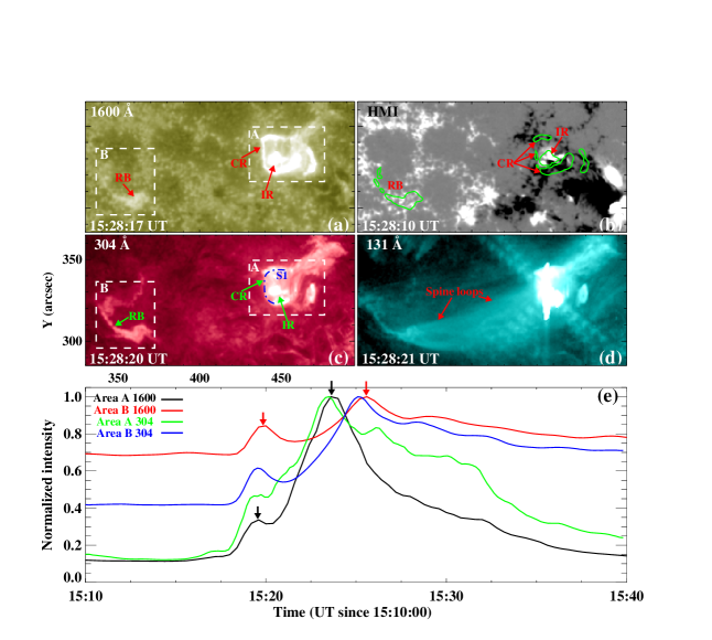
Figure 1: Overview of the M1.8 circular-ribbon flare on 2016 February 13 in AR 12497 including the multi-wavelength images from SDO/AIA, SDO/HMI LOS magnetogram, and lightcurves of the flare. CR, IR and RB respectively denote the circular ribbon, inner ribbon and remote brightenings. The two areas A and B in panels (a) and (c) enclose the flare core region and the remote brightening region. The green curves in panel (b) are the brightness contours of the three ribbons in the AIA 1600 Å image. The blue dash-dotted curve “S1” in panel (c) shows the cut position used to obtain the time-distance plot shown in Figure 3(c). The lightcurves in panel (e) are normalised to 1, and black and red arrows point to two peaks of the 1600 Å lightcurves within areas A and B.

On 2016 February 13, an M1.8 confined circular-ribbon flare occurred in AR 12497 (N14, W28), which was initiated at 15:16 UT and peaked at 15:24 UT from the GOES SXR 1$-$8 Å flux data. Three flare ribbons were distinguished from the SDO multi-wavelength observations, including a quasi-circular ribbon (noted CR in Figures 1(a)-(c)), an inner ribbon (IR) and remote brightenings (RB) at the east. The comparison of 1600 Å images with HMI LOS magnetograms showed that the ribbon IR was located at the central positive-polarity region (parasitic polarity) and CR anchored in the surrounding negative-polarity fields (Figure 1(b)). The evolution of photospheric magnetic fields showed that new flux emergence within the leading negative-polarity of the AR over one day prior resulted in the formation of this parasitic polarity. The third ribbon RB extended northward as the flare developed, and it resided at the trailing positive region of the AR. As seen from the high-temperature 131 Å observations (about 11 MK; O’Dwyer et al. 2010), a hot loop bundle appeared about 1 min after the formation of RB, with its eastern end mapping to RB and the western end to the main flaring region (Figure 1(d)). The loop bundle probably traced the spine field lines in the fan-spine topology, and thus was name as “spine loops” (Sun et al. 2013).

In order to examine how the UV and EUV emissions varied with time, we calculated the 1600 Å and 304 Å lightcurves of the event. The normalised magnitudes of the lightcurves within the main flaring region “A” and remote brightening region “B” are presented in Figure 1(e). Interestingly, there are two peaks in the four lightcurves for both areas “A” and “B”. The 1600 Å emission in area “A” started to increase rapidly from around 15:17:50 UT and reached its first peak at 15:19:30 UT (black curve). Then the UV emission decreased slightly before the second rise phase. The second peak occurred at 15:23:40 UT, consistent with the GOES SXR 1$-$8 Å flux. The time interval between the two peaks is about 4 min and the first small peak is nearly 30 % of the second peak. The 304 Å time profile in area “A” (green curve) has a similar variation with the 1600 Å curve. Differently, the first peak in 304 Å lightcurve has a stronger emission than that in 1600 Å radiation, about 50 % of the second peak. The emissions of the remote brightenings RB also show two phases (red and blue curves). The RB observed at 1600 Å was formed about 20 s later than the circular ribbon CR (red and black curves), and the first peak occurred at 15:19:50 UT. The second phase of RB started with a 70 s delay relative to the appearance of the second CR. The RB reached its strongest emission at about 15:25:35 UT and then decayed gradually. For the 304 Å time profile of RB (blue curve), the second peak has a larger emission enhancement above the background, compared with the 1600 Å profile.

3.2 Two Episodes of the Flare Evolution

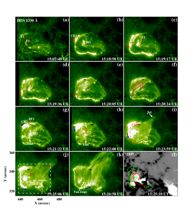
Figure 2: Time sequences of IRIS 1330 Å images showing two episodes of the evolution of circular ribbons (see Animation 1330-flare). Two dash-dotted curves in panel (a) outline two filament structures F1 and F2 prior to the flare, and their duplications are also plotted in panel (l). CR1 and IR1 in panel (b) denote the first circular and inner ribbons, and red arrows in panels (b)-(e) represent the elongation motion of CR1. The dashed and solid curves in panels (c)-(f) denote the successive appearance of the erupting F1. CR2 and IR2 in panel (g) are the second circular and inner ribbons, and blue arrows in panels (g)-(j) indicate the elongation motion of CR2. BF2 in panel (g) denotes the initial brightening of F2. The red dash-dotted curve “S2” in panel (i) shows the cut position used to obtain the time-distance plot shown in Figure 3(b). Areas C and D in panel (j) mark the FOVs within which the lightcurves in Figure 3(a) are obtained. The green curves in panel (l) are the brightness contours of CR2 and IR2 at 15:25:06 UT.

By analyzing the IRIS high-resolution observations in detail, we find that two distinct episodes of energy release are involved in the impulsive phase of the flare. Before the onset of the flare, two filament structures (F1 and F2) existed along the eastern and southern portions of the quasi-circular polarity inversion line (PIL) (Figures 2(a) and 2(l)). The lengths of F1 and F2 were about 30$\arcsec$, the typical length of mini-filaments (Hermans & Martin 1986; Hong et al. 2017; Shen et al. 2017). The northern ends of F1 and F2 were located at the central positive-polarity magnetic fields and their southern ends anchored in the neighboring negative-polarity fields. From about 15:18:10 UT, some faint brightenings of the first circular ribbon (CR1) started to appear at the northeast part (see Animation 1330-flare). Then the brightenings of CR1 were enhanced and exhibited a slow elongation motion towards the south (Figure 2(b)). Meanwhile, the brightenings of the first inner ribbon (IR1) evolved to the south, similar to the dynamic evolution of CR1. About 1 min after the appearance of CR1, the filament F1 was brightened and began to rise up with a velocity of about 110 km s^-1 (Figure 2(c)). The eastern end of F1 exhibited an apparent slipping motion and the western end was located at the vicinity of the IR1 (Figures 2(d)-(f)). These successively brightened structures of F1 delineated a curved surface (Figure 2(f)), implying the existence of a QSL surrounding the filament F1 (Li & Zhang 2014; Li et al. 2017c). Associated with the fast expansion of F1, the elongation motion of CR1 became faster in the counterclockwise direction (red arrows in Figures 2(c)-(e)). As the CR1 traveled south, the brightenings of CR1 clearly jumped to the west (see Figures 2(b)-(f) and Animation 1330-flare). This suggested that the filament F1 had been reconnected with open field via null-point reconnection and the brightenings of CR1 followed the sequential opening of F1.

From about 15:21:03 UT, the north part of the filament F2 was associated with evident brightenings (BF2 in Figure 2(g)), implying the onset of the second episode of magnetic reconnections. About 20 s later, the brightenings of the second circular ribbon (CR2) started to appear at the periphery of BF2 (Figure 2(g)). The filament F2 underwent a slipping eruption with the south end propagating towards the west at a speed of about 40 km s^-1 (Figures 2(g)-(h)). The eruption of F2 was also accompanied by a counterclockwise rotating motion. Simultaneously, the circular ribbon CR2 and the second inner ribbon (IR2) were both brightened sequentially in the counterclockwise direction with respective speeds of 60 and 40 km s^-1 (Figures 2(g)-(k)). The dynamic evolution of CR2 is consistent with that of CR1, while the emission intensity and the width of CR2 are much larger than those of CR1. In the late phase, the erupting F2 formed a curtain-like, blowout jet after 15:23:59 UT (Figures 2(i)-(k)). The jet seemed to consist of thread-like fine structures, which probably traced out the fan loops in the fan-spine topology (Figure 2(k)). The fan loops also exhibited an apparent slipping motion towards the west and their footpoints corresponded to the evolving bright dots within CR2. Associated with the westward motion of the CR2, its brightenings along the south side shifted significantly northward (compared with the former faint brightenings at the south in Figure 2(h)). This indicated that the filament F2 was reconnected with open field via null-point reconnection and thus the fan plane separatrix footprint followed the path of F2 (Wyper et al. 2017).

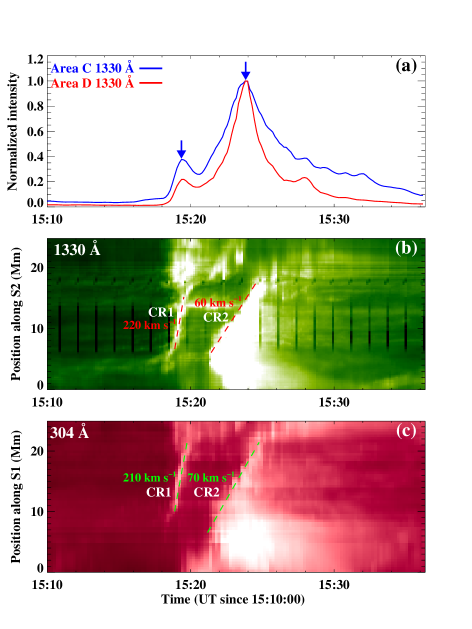
Figure 3: Panel (a): normalised lightcurves of IRIS 1330 Å within areas C and D (Figure 2(j)). Blue arrows point to two peaks of the emission within area C. Panel (b): time-distance plot along slice “S2” (red dash-dotted curve in Figure 2(i)) in the 1330 Å passband. Panel (c): time-distance plot along slice “S1” (blue dash-dotted curve in Figure 1(c)) in the 304 Å passband.

To present how the 1330 Å emission varied in time, we calculated the lightcurves within the main flaring region “C” and its subregion “D” (Figure 2(j)) and plotted the normalised magnitudes of the lightcurves in Figure 3(a). From about 15:18:20 UT, the emission within area “C” increased rapidly, corresponding to the appearance of CR1 and the initiation of the first episode of magnetic reconnections. The first phase lasted about 130 s, with the peak at about 15:19:20 UT (first blue arrow). The second peak occurred at about 15:23:50 UT (second blue arrow), which was separated by a 270 s time delay. The second phase had stronger emissions than the first phase, with the second peak flux nearly a factor of 2.5 larger. The curves “C” and “D” were very similar and both had two distinct phases, implying that the inner ribbons were co-temporal with the circular ribbons. In order to analyze the elongation motions of the circular ribbons, we obtain two stack plots (Figures 3(b)-(c)) respectively along slice “S2” in 1330 Å images (red curve in Figure 2(i)) and slice “S1” in 304 Å images (blue curve in Figure 1(c)). As seen from the 1330 Å stack plot, the initial elongation motion of CR1 was relatively slow in the first tens of seconds. Then the ribbon CR1 extended rapidly toward the south with a larger velocity of about 220 km s^-1. About 1 min after the disappearance of CR1, CR2 was generated and subsequently propagated in the counterclockwise direction at a smaller velocity of 60 km s^-1. The 304 Å stack plot showed a similar result that CR1 propagated at a velocity nearly a factor of three faster compared to CR2.

3.3 Dynamics of the Overlying Loops

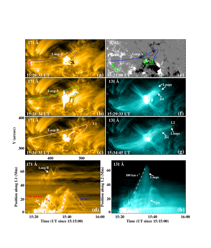
Figure 4: SDO/AIA 171 Å and 131 Å observations showing the expansions and oscillations of coronal loops overlying the flaring region (see Animation EUV-loops). The blue and green curves in panels (a)-(b) and (e) outline the locations of loop “A” at different times. White solid and dotted curves in panels (c)-(d) denote the loop “B” and its oscillation behavior. Red and dark contours in panel (a) are the magnetic fields at $\pm$400 G levels at the ends of loop “A”. Panel (d) shows the time-distance plot along slice “L1” (red dash-dotted line in panel (c)) in the 171 Å passband. The red and blue dashed lines in panel (d) respectively indicate the ejecting and falling materials from the blowout jet. The green contours in panel (e) are the brightness of flare ribbons in the 1600 Å channel. Panel (h) shows the time-distance plot along slice “L2” (brown dash-dotted line in panel (g)) in the 131 Å passband. The white dashed line in panel (h) denotes the expansion motion of the overlying loops.

In the 171 Å and 131 Å images, many long and high coronal loops were observed above the flare (Figure 4 and Animation EUV-loops). The HMI magnetograms and 171 Å images showed that the eastern footpoints of the loop bundle anchored in the positive-polarity fields at the northeast of remote brightenings RB and their western footpoints in the peripheral negative-polarity fields of the circular ribbons (Figures 4(a) and (e)). Two loop structures “A” and “B” were traced to investigate their dynamic evolution (Figures 4(a)-(c)). Associated with the ascent of the blowout jet, loop “A” was pushed upward and its projected height increased by about 9 Mm in about 8 min (Figures 4(a)-(b)). While loop “B” showed the oscillation pattern as seen from the stack plot along slice “L1” (Figures 4(c)-(d)). The oscillation had an average period of 4 min, in agreement with the typical periods of several minutes for the kink oscillations of coronal loops (Liu & Ofman 2014; Zimovets & Nakariakov 2015; Li et al. 2017a). The rising speed of the jet was estimated to be 140$-$160 km s^-1 and the maximum height traced was up to 40 Mm (Figure 4(d)). Due to strong constraints of overlying loops, the erupting materials from the blowout jet finally fell back to the solar surface with a velocity of about 50 km s^-1. By examining the data from the Large Angle and Spectrometric Coronagraph (LASCO) Experiment, we found that the circular-ribbon flare did not produce any CMEs and evolved into a confined event. In 131 Å images, the upward expansion of bushy high-temperature coronal loops was detected above the jet front (Figures 4(f)-(g)). The displacement of these expanding loops reached about 38 Mm and the speed was about 100 km s^-1, smaller than the rising speed of ejecting materials (Figure 4(h)). Eventually, the high-temperature loops gradually cooled down and can not be discerned in 131 Å images.

3.4 Fan-spine Magnetic Topology of Flaring Region

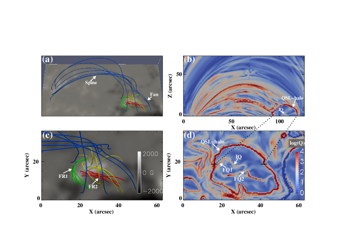
Figure 5: Panel (a): side view of the extrapolated field lines at 15:00 UT showing the fan-spine topology. The background shows the photospheric vertical magnetic field. Panel (b): distribution of the squashing factor Q in the x-z plane obtained from the NLFFF field, which depicts the QSL-halo around the separatrix (fan) and the IQ surrounding the inner spine field lines. Panel (c): top view of the zoomed image of panel (a). FR1 and FR2 are two flux ropes underlying the fan dome. Panel (d): logarithm Q on the bottom boundary. FQ1 and FQ2 denote two flux-rope-related QSLs within the QSL-halo.

The extrapolation results show the existence of a fan-spine topology prior to the flare (Figure 5). The fan structure divides the coronal volume in two connectivity domains, the inner and the outer connectivity domain. The field lines in inner domain are connected with the central parasitic positive-polarity region (yellow lines in Figure 5(a)), and the field lines in outer domain link with remote positive-polarity region (blue lines). As seen from the distribution of the Q factor (Figure 5(b)), a dome-shaped QSL structure (referred to as a “QSL-halo” in Masson et al. 2009) outlining the fan plane and another QSL structure (IQ) outlining the inner spine inside the dome are present. Under the fan dome, two flux ropes (FR1 and FR2) are present respectively along the eastern and southern parts of the quasi-circular PIL (green and red lines in Figure 5(c)). FR1 consists of moderately twisted field lines with the average twist number of 1.1 (Berger & Prior 2006; Liu et al. 2016). Compared to Figure 2, FR1 bears a good resemblance to the observed filament F1. The south flux rope FR2 is weakly twisted with the average twist number of about 0.6, which probably corresponds to the south part of the filament F2. In the top view of the Q map (Figure 5(d)), the intersection of the QSL-halo with the lower boundary forms a quasi-circular morphology that approximately overlaps the location of circular ribbons CR1 and CR2 (Figures 2 and 5). Besides the two QSL structures (QSL-halo and IQ) around the fan-spine topology, two flux-rope-related QSLs (FQ1 and FQ2) exist inside the QSL-halo, respectively binding FR1 and FR2. The combination of the extrapolated results and the observations shows that the curved surface delineated by the eruption of F1 may correspond to the FQ1 (Figures 2(f) and 5(d)) and the slipping motion of F2 during the second episode is probably along the FQ2 (Figures 2(g)-(h) and 5(d)).

4 Summary and Discussion

We have examined a special M1.8 circular-ribbon flare on 2016 February 13. The flare accompanied by the eruptions of multiple filaments and exhibited two distinct episodes of magnetic reconnections. The UV and EUV emissions of the flaring region showed two peaks with an interval of about 270 s, of which the second peak was energetically more important. The first episode was associated with the eruption of a mini-filament F1 and the fast elongation motion of a thin circular ribbon CR1. The eastern end of the erupting F1 exhibited an apparent slipping motion towards the south, with the rising speed reaching about 110 km s^-1. Accompanied by the fast expansion of F1, the ribbon CR1 brightened sequentially in the counterclockwise direction at a rapid speed of about 220 km s^-1. The two spine-related ribbons (IR1 and RB) were simultaneously elongated. In the second episode, another mini-filament F2 erupted and the second circular ribbon CR2 was formed at the same location of CR1. The broad ribbon CR2 and inner ribbon IR2 also showed counterclockwise elongation motions with respective speeds of 60 and 40 km s^-1. The erupting F2 finally developed into a blowout jet and the thread-like fine structures of the jet traced out the fan loops. The jet caused the upward expansion of the high-temperature coronal loops above the flare at a speed of about 100 km s^-1. Due to the strong constraints of overlying coronal loops, the flare became a confined event and did not generate any CMEs.

The extrapolated 3D coronal magnetic fields reveal the existence of a fan-spine topology. A dome-shaped QSL-halo outlining the fan surface and another QSL structure around the inner spine are present. The intersection of the QSL-halo with the lower boundary is approximately co-spatial with circular ribbons CR1 and CR2. Two flux ropes and two flux-rope-related QSLs exist under the fan dome, which roughly correspond to the two filaments F1 and F2 and two respective QSLs binding them. In each episode, the sequential brightenings of the circular ribbon and two spine-related ribbons indicate the shifts of the fan plane footprint and the footpoints of both spines. A relevant simulation study was carried out by Wyper et al. (2016), who showed that during a confined eruption the inner and outer spines shift rapidly across the photosphere (see their Figure 11 and the related movie), concurrent with a shifting of the fan plane footprint. In that study, the field beneath the fan plane was sheared, rather than including a filament, however those authors have recently updated their model to include a filament (Wyper et al. 2017, 2018). A similar shift in spine and fan footpoints occurs as the filament erupts and is reconnected on to open field. Our observations are similar to their simulation studies, and show that the erupting filaments probably lead to significant shifts of the fan plane footprint via the null-point reconnection.

By comparing our results with the numerical studies of Wyper et al. (2017, 2018), we propose a compound eruption model of circular-ribbon flares consisting of two sets of successively formed ribbons and eruptions of multiple filaments in a fan-spine-type magnetic configuration. A simple schematic picture is shown in Figure 6. First, the null-point reconnection between the outermost flux of the filament F1 (blue curves) and the ambient open field occurs (panel (a)), which transfers partial flux of F1 to the closed field under the far side of the dome and to the open field exterior to the near side of the dome (dashed cyan lines in panel (a)). Meanwhile, the circular ribbon CR1 and inner ribbon IR1 (orange curves) are generated due to the flow of reconnection-accelerated particles from the null along the fan plane and the spine field into the lower atmosphere. The null-point reconnection is likely of the breakout nature (Antiochos et al. 1999; Wyper et al. 2017, 2018). Then the F1 undergoes the slipping magnetic reconnection along the QSL binding the F1, which induces the far flux of F1 reaching the null point (panel (b)). The continuous null-point reconnection causes the sequential opening of F1, and thus leads to the significant shifts of the brightenings of CR1 and IR1 (orange regions in panel (b)). In the first episode, partial flux is transferred from under the separatrix dome via the null-point reconnection, which effectively alleviates the constraint of the nearby filament F2 (green curves). Later on, the stability of F2 is disrupted and the second episode of the flare is initiated. The continuous null-point reconnection between F2 and open field is at work and generates the sequential brightenings of CR2 and IR2 (panels (c)-(d)), similar to the evolution of the first episode. Meanwhile, the blowout jet is formed as filament material below the separatrix is ejected along field lines outside the separatrix.

Besides the null-point reconnection, we suggest that slipping magnetic reconnection along the extended QSL-halo is also involved in the flare. The elongation speeds of the two circular ribbons (60 and 220 km s^-1) are sub-Alfvénic, satisfying the slipping reconnection regime according to Aulanier et al. (2006). Pontin et al. (2016) analyzed the distribution of Q in the presence of magnetic nulls and demonstrated that the extended QSL-halo was a generic feature for a non-radially-symmetric null. Slipping reconnection along the QSL-halo is a natural element of 3D null-point reconnection and occurs any time 3D null reconnection occurs (Masson et al. 2009, Reid et al. 2012). We suggest that the null-point and slipping magnetic reconnections are both at work in the two episodes of the flare, with the second episode being more violent and releasing more magnetic energy. Slipping reconnection leads to a continuous change of connectivity across QSL, while null-point reconnection leads to a jump of connectivity and thus to a flux transfer through separatrices.

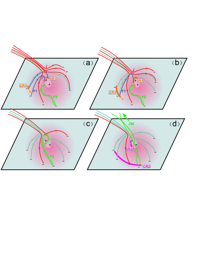
Figure 6: Schematic of the compound eruption process. Red lines show the open field lines of the fan dome. Blue and green lines respectively represent the two filaments F1 and F2 under the separatrix. At the null, the filament and ambient open field lines undergo breakout-type reconnection. Dashed cyan lines denote the newly formed open fields exterior to the near side of the dome and the closed fields under the far side of the dome. The circular ribbon CR1 and inner ribbon IR1 in the first episode are shown by orange in panels (a)-(b). The orange arrows represent the sequential brightenings of CR1 and IR1. The magenta lines in panel (d) denote the circular ribbon CR2 and inner ribbon IR2 in the second episode.

References

- (1) Antiochos, S. K. 1998, ApJ, 502, L181
- (2) Antiochos, S. K., DeVore, C. R., & Klimchuk, J. A. 1999, ApJ, 510, 485
- (3) Aulanier, G., Golub, L., DeLuca, E. E., et al. 2007, Science, 318, 1588
- (4) Aulanier, G., Janvier, M., & Schmieder, B. 2012, A&A, 543, A110
- (5) Aulanier, G., Pariat, E., Démoulin, P., & DeVore, C. R. 2006, Sol. Phys., 238, 347
- (6) Berger, M. A., & Prior, C. 2006, Journal of Physics A Mathematical General, 39, 8321
- (7) Bobra, M. G., Sun, X., Hoeksema, J. T., et al. 2014, Sol. Phys., 289, 3549
- (8) Chandra, R., Schmieder, B., Mandrini, C. H., et al. 2011, Sol. Phys., 269, 83
- (9) Cheng, X., Guo, Y., & Ding, M. 2017, Science in China Earth Sciences, 60, 1383
- (10) Démoulin, P., Bagala, L. G., Mandrini, C. H., Henoux, J. C., & Rovira, M. G. 1997, A&A, 325, 305
- (11) Démoulin, P., Priest, E. R., & Lonie, D. P. 1996, J. Geophys. Res., 101, 7631
- (12) De Pontieu, B., Title, A. M., Lemen, J. R., et al. 2014, Sol. Phys., 289, 2733
- (13) Dudík, J., Janvier, M., Aulanier, G., et al. 2014, ApJ, 784, 144
- (14) Dudík, J., Polito, V., Janvier, M., et al. 2016, ApJ, 823, 41
- (15) Fletcher, L., Metcalf, T. R., Alexander, D., Brown, D. S., & Ryder, L. A. 2001, ApJ, 554, 451
- (16) Forbes, T. G., Linker, J. A., Chen, J., et al. 2006, Space Sci. Rev., 123, 251
- (17) Gorbachev, V. S., Kelner, S. R., Somov, B. V., & Shvarts, A. S. 1988, Soviet Ast., 32, 308
- (18) Green, L. M., Kliem, B., & Wallace, A. J. 2011, A&A, 526, A2
- (19) Hao, Q., Yang, K., Cheng, X., et al. 2017, Nature Communications, 8, 2202
- (20) Hermans, L. M., & Martin, S. F. 1986, BAAS, 18, 991
- (21) Hernandez-Perez, A., Thalmann, J. K., Veronig, A. M., et al. 2017, ApJ, 847, 124
- (22) Hong, J., Jiang, Y., Yang, J., Li, H., & Xu, Z. 2017, ApJ, 835, 35
- (23) Hou, Y. J., Li, T., & Zhang, J. 2016, A&A, 592, A138
- (24) Janvier, M., Aulanier, G., Pariat, E., & Démoulin, P. 2013, A&A, 555, A77
- (25) Jiang, C., Feng, X., Wu, S. T., & Hu, Q. 2013, ApJ, 771, L30
- (26) Jiang, F., Zhang, J., & Yang, S. 2015, PASJ, 67, 78
- (27) Jing, J., Liu, R., Cheung, M. C. M., et al. 2017, ApJ, 842, L18
- (28) Joshi, N. C., Liu, C., Sun, X., et al. 2015, ApJ, 812, 50
- (29) Lau, Y.-T., & Finn, J. M. 1990, ApJ, 350, 672
- (30) Lemen, J. R., Title, A. M., Akin, D. J., et al. 2012, Sol. Phys., 275, 17
- (31) Li, D., Ning, Z. J., Huang, Y., et al. 2017a, ApJ, 849, 113
- (32) Li, H., Jiang, Y., Yang, J., et al. 2017b, ApJ, 836, 235
- (33) Li, T., Yang, K., Hou, Y., & Zhang, J. 2016, ApJ, 830, 152
- (34) Li, T., & Zhang, J. 2014, ApJ, 791, L13
- (35) Li, T., & Zhang, J. 2015, ApJ, 804, L8
- (36) Li, T., Zhang, J., & Hou, Y. 2017c, ApJ, 848, 32
- (37) Liu, C., Deng, N., Liu, R., et al. 2015, ApJ, 812, L19
- (38) Liu, R., Kliem, B., Titov, V. S., et al. 2016, ApJ, 818, 148
- (39) Liu, W., Berger, T. E., Title, A. M., Tarbell, T. D., & Low, B. C. 2011, ApJ, 728, 103
- (40) Liu, W., & Ofman, L. 2014, Sol. Phys., 289, 3233
- (41) Longcope, D. W. 1996, Sol. Phys., 169, 91
- (42) Mandrini, C. H., Demoulin, P., Bagala, L. G., et al. 1997, Sol. Phys., 174, 229
- (43) Mandrini, C. H., Schmieder, B., Démoulin, P., Guo, Y., & Cristiani, G. D. 2014, Sol. Phys., 289, 2041
- (44) Masson, S., Pariat, E., Aulanier, G., & Schrijver, C. J. 2009, ApJ, 700, 559
- (45) Masson, S., Pariat, É., Valori, G., et al. 2017, A&A, 604, A76
- (46) Moreno-Insertis, F., Galsgaard, K., & Ugarte-Urra, I. 2008, ApJ, 673, L211
- (47) O’Dwyer, B., Del Zanna, G., Mason, H. E., Weber, M. A., & Tripathi, D. 2010, A&A, 521, A21
- (48) Pesnell, W. D., Thompson, B. J., & Chamberlin, P. C. 2012, Sol. Phys., 275, 3
- (49) Pontin, D., Galsgaard, K., & Démoulin, P. 2016, Sol. Phys., 291, 1739
- (50) Pontin, D. I., Priest, E. R., & Galsgaard, K. 2013, ApJ, 774, 154
- (51) Priest, E. R., & Démoulin, P. 1995, J. Geophys. Res., 100, 23443
- (52) Priest, E. R., & Forbes, T. G. 2002, A&A Rev., 10, 313
- (53) Priest, E. R., & Titov, V. S. 1996, Philosophical Transactions of the Royal Society of London Series A, 354, 2951
- (54) Reid, H. A. S., Vilmer, N., Aulanier, G., & Pariat, E. 2012, A&A, 547, A52
- (55) Scherrer, P. H., Schou, J., Bush, R. I., et al. 2012, Sol. Phys., 275, 207
- (56) Shen, Y., Liu, Y., Tian, Z., & Qu, Z. 2017, ApJ, 851, 101
- (57) Shibata, K., & Magara, T. 2011, Living Reviews in Solar Physics, 8, 6
- (58) Sun, X., Hoeksema, J. T., Liu, Y., et al. 2013, ApJ, 778, 139
- (59) Titov, V. S., Hornig, G., & Démoulin, P. 2002, Journal of Geophysical Research (Space Physics), 107, 1164
- (60) Török, T., Aulanier, G., Schmieder, B., Reeves, K. K., & Golub, L. 2009, ApJ, 704, 485
- (61) Wang, H. 1997, Sol. Phys., 174, 265
- (62) Wang, H., & Liu, C. 2012, ApJ, 760, 101
- (63) Wheatland, M. S., Sturrock, P. A., & Roumeliotis, G. 2000, ApJ, 540, 1150
- (64) Wiegelmann, T. 2004, Sol. Phys., 219, 87
- (65) Wiegelmann, T., Inhester, B., & Sakurai, T. 2006, Sol. Phys., 233, 215
- (66) Wyper, P. F., Antiochos, S. K., & DeVore, C. R. 2017, Nature, 544, 452
- (67) Wyper, P. F., DeVore, C. R., & Antiochos, S. K. 2018, ApJ, 852, 98
- (68) Wyper, P. F., DeVore, C. R., Karpen, J. T., & Lynch, B. J. 2016, ApJ, 827, 4
- (69) Xu, Z., Yang, K., Guo, Y., et al. 2017, ApJ, 851, 30
- (70) Xue, Z., Yan, X., Yang, L., Wang, J., & Zhao, L. 2017, ApJ, 840, L23
- (71) Yan, X. L., Jiang, C. W., Xue, Z. K., et al. 2017, ApJ, 845, 18
- (72) Yang, K., Guo, Y., & Ding, M. D. 2015, ApJ, 806, 171
- (73) Yang, S., Zhang, J., Zhu, X., & Song, Q. 2017, ApJ, 849, L21
- (74) Zhang, Q. M., Li, D., Ning, Z. J., et al. 2016a, ApJ, 827, 27
- (75) Zhang, Q. M., Li, D., & Ning, Z. J. 2016b, ApJ, 832, 65
- (76) Zheng, R., Chen, Y., & Wang, B. 2016, ApJ, 823, 136
- (77) Zimovets, I. V., & Nakariakov, V. M. 2015, A&A, 577, A4