Global Nonlinear Normal Modes in
the Fullerene Molecule $C_{60}$

Abstract

In this paper we analyze nonlinear dynamics of the fullerene molecule. We prove the existence of global branches of periodic solutions emerging from an icosahedral equilibrium (nonlinear normal modes). We also determine the symmetric properties of the branches of nonlinear normal modes for maximal orbit types. We find several solutions which are standing and rotating waves that propagate along the molecule with icosahedral, tetrahedral, pentagonal and triangular symmetries. We complement our theoretical results with numerical computations using Newton’s method.

1 Introduction

The fullerene molecule was discovered in 1986 by R. Smalley, R. Curl, J. Heath, S. O’Brien, and H. Kroto, and since then continues to attract great deal of attention in the scientific community (e.g. the original work [22] has currently 15 thousand citations). Its importance led in 1996 to awarding the Nobel prize in chemistry to Smalley, Curl and Kroto. Since its discovery, applications of fullerene C60 have been extensively explored in biomedical research due to their unique structure and physicochemical properties.

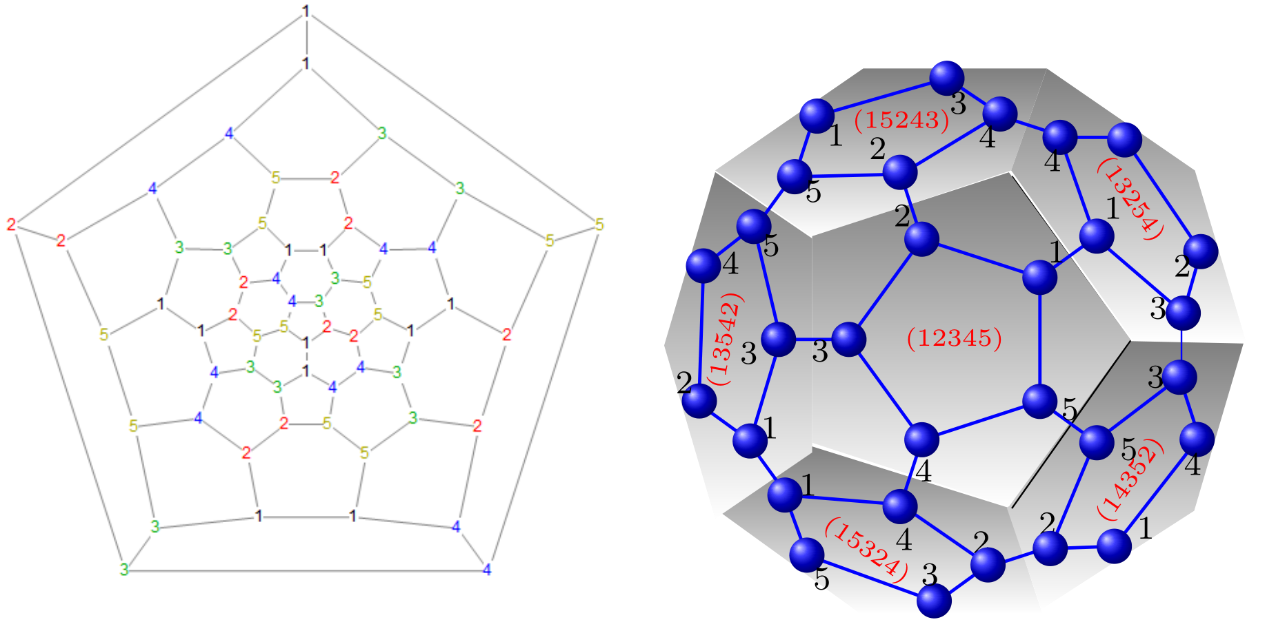
Figure 1: The fullerene molecule

The fullerene molecule is composed of $60$ carbon atoms at the vertices of a truncated icosahedron (see Figure 1). Various mathematical models for the fullerene molecule are built in the framework of classical mechanics. Many force fields have been proposed for the fullerene in terms of bond stretching, bond bending, torsion and van der Waals forces. Some force fields were optimized to duplicate the normal modes obtained using IR or Raman spectroscopy, but only few of these models reflect the nonlinear characteristics of the fullerene. For instance, the force field implemented in [33] for carbon nanotubes and in [6] for the fullerene, assumes bond deformations that exceed very small fluctuations about equilibrium states, while the force fields proposed in [34] and [37] are designed only to consider small fluctuations in the fullerene model. Although the linear vibrational modes of fullerene can be measured using IR and Raman spectroscopy, increasing attention has been given to the mathematical study of other vibrational modes that cannot be measured experimentally (see [16, 8, 20, 33, 34, 37, 30] and the large bibliography therein).

Mathematical Models.

In molecular dynamics, a fullerene molecule model consists of a Newtonian system

$$m\ddot{u}=-\nabla V(u),$$ (1)

where the vector $u(t)\in\widetilde{\mathscr{V}}:=\mathbb{R}^{180}$ represents the positions of 60 carbon atoms in space, $m$ is the carbon mass (which by rescaling the model can be assumed to be one) and $V(u)$ is the energy given by a force field. This force field is symmetric with respect to the action of the group $\Gamma:=I\times O(3)$, where $I$ denotes the full icosahedral group. This important property allows application of various equivariant methods to analyze its dynamical properties. In order to make the system (1) reference point-depended, we define the subspace $\mathscr{V}$ of $\mathbb{R}^{180}$ by

$$\mathscr{V}:=\{x=(x_{1},x_{2},\dots,x_{60}):x_{k}\in\mathbb{R}^{3},\;\sum_{k=1}^{60}x_{k}=0\},$$ (2)

from which we exclude the collision orbits, i.e. we consider the restriction of the system (1) to the set $\Omega_{o}:=\{x\in\mathscr{V}:x_{j}\not=x_{k},\;j\not=k\}$.

Analysis of Nonlinear Molecular Vibrations.

The mathematical analysis of a molecular model includes two objectives: identification of the normal frequencies and the classification of different families of periodic solutions with various spatio-temporal symmetries emerging from the equilibrium configuration of the molecule (nonlinear normal modes). Let us emphasize that the classification of normal modes is a central problem of the molecular spectroscopy.

The study of periodic orbits in Hamiltonian systems can be traced back to Poincare and Lyapunov, who proved the existence of nonlinear normal modes (periodic orbits) near an elliptic equilibrium under non-resonant conditions. Later on, Weinstein (cf. [35]) extended this result to the case with resonances. However, in general, the existence of nonlinear normal modes is not guaranteed under the presence of resonances. Indeed, Moser presented in [24] an example of a Hamiltonian systems with resonances, where the linear system is full of periodic solutions, but the nonlinear system has none.

Let us point out that due to the icosahedral symmetries, the fullerene molecule $C_{60}$ has resonances of multiplicities 3, 4 and 5, i.e. the existence of linear modes does not guarantee the existence of nonlinear normal modes in fullerene $C_{60}$ due to resonances. Therefore, one needs a good method that takes in consideration these symmetries. Standard methods for such analysis may use reductions to the $H$-fixed point spaces, normal form classification, center manifold theorem, averaging method and/or Lyapunov–Schmidt reduction.

Variational Reformulation.

The problem of finding periodic solutions for the fullerene can be reformulated as a variational problem on the Sobolev space $H_{2\pi}^{1}(\mathbb{R};{\mathscr{V}})$ (of $2\pi$-periodic ${\mathscr{V}}$-valued functions) with the functional

$$J_{\lambda}(u):=\int_{0}^{2\pi}\left[\frac{1}{2}|\dot{u}(t)|^{2}-\lambda^{2}V(u(t))\right]dt,\quad u\in H_{2\pi}^{1}(\mathbb{R};\Omega_{o}),$$

where $V$ is the force field, $\lambda^{-1}$ the frequency and $u$ the renormalized $2\pi$-periodic solution. The existence of periodic solutions (with fixed frequency $\lambda^{-1}$) is equivalent to the existence of critical points of $J_{\lambda}$. It follows from the construction of the force field that the functional $J_{\lambda}$ is invariant under the action of the group

$$G:=\Gamma\times O(2)=(I\times O(3))\times O(2),$$

which acts as permutations of atoms, rotations in space, and translations and reflection in time, respectively.

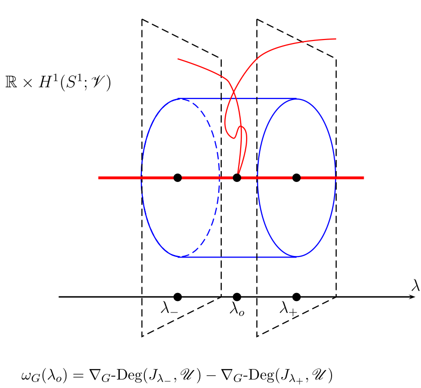
Figure 2: Local bifurcation.

Gradient Equivariant Degree Method.

To provide an alternative to the equivariant singularity theory (cf. [14]) and other geometric methods that have been used to analyze molecules (see [17], [19], [23] and references), we proposed (see [11, 5, 4]) the method based on the equivariant gradient degree (fundamental properties of the gradient equivariant degree are collected in Appendix A) – a generalization of the Brouwer/Leray-Schauder degree that was developed in [12] for the gradient maps (see also [9] and [29]). The gradient equivariant degree is just one of many equivariant degrees that were introduced in the last three decades for various types of differential equations (see [2], [3], [18], [21] and references therein).

To describe the main idea of this method, let us point out that the gradient equivariant degree satisfies all the standard properties expected from a degree theory (i.e. existence, additivity, homotopy and multiplicativity properties). The $G$-equivariant gradient degree $\nabla_{G}\text{-Deg}(\nabla J_{\lambda},\mathscr{U})$ of $\nabla J_{\lambda}$ on $\mathscr{U}$ can be expressed elegantly as an element of the Euler ring $U(G)$ (which is the free $\mathbb{Z}$-module generated by the conjugacy classes $(H)$ of closed subgroups $H\leq G$) in the form

$$\nabla_{G}\text{-Deg}(\nabla J_{\lambda},\mathscr{U})=n_{1}(H_{1})+n_{2}(H_{2})+\dots+n_{m}(H_{m}),\;\;\;n_{k}\in\mathbb{Z},$$

where $\mathscr{U}$ is a neighborhood of the $G$-orbit of the equilibrium $u_{o}$ (for some non-critical frequency $\lambda^{-1}$) and $(H_{j})$ are the orbit types in $\mathscr{U}$. The changes of $\nabla_{G}\text{-deg}(\nabla J_{\lambda},\mathscr{U})$ when $\lambda^{-1}$ crosses a critical frequency $\lambda_{o}^{-1}$ allow to establish the existence of various families of orbits of periodic molecular vibrations and their symmetries emerging from an equilibrium. In fact, the equivariant topological invariant

$$\omega_{G}(\lambda_{o}):=\nabla_{G}\text{-Deg\thinspace}(\nabla J_{\lambda_{-}},\mathscr{U})-\nabla_{G}\text{-Deg\thinspace}(\nabla J_{\lambda_{+}},\mathscr{U})$$ (3)

provides a full topological characterization of the families of periodic solutions (together with their symmetries) emerging from an equilibrium at $\lambda_{o}$ (cf. [10]). More precisely, for every non-zero coefficient $m_{j}$ in

$$\omega_{G}(\lambda_{o})=m_{1}(K_{1})+m_{2}(K_{2})+\dots m_{r}(K_{r}),$$

there exists a global family of periodic molecular vibrations with symmetries at least $K_{j}$ (see Figure 2 below). Moreover, if $(K_{j})$ is a maximal orbit type then this family has exact symmetries $K_{j}$.

Global Bifurcation Result.

The so-called classical Rabinowitz Theorem [27] establishes occurrence of a global bifurcation from purely local data for compact perturbations of the identity. Its main idea is that if the maximal connected set $\mathcal{C}$ bifurcating from a trivial solution is compact (i.e. bounded), then the sum of the local Leray-Schauder degrees at the set of bifurcation points of $\mathcal{C}$ is zero. Since such maximal connected set $\mathcal{C}$ is either unbounded or comes back to another bifurcation point, this result is also referred to as the global Rabinowitz alternative (we refer to Nirenberg’s book [26] where a simplified proof of this statement is presented in Theorem 3.4.1).

The classical Rabinowitz’s global bifurcation argument can be easily adapted in the equivariant setting for the gradient $G$-equivariant degree (cf. [13]). That is, for any $G$-orbit of a compact (bounded) branch $\mathcal{C}$ in $\mathbb{R}_{+}\times H_{2\pi}^{1}(\mathbb{R};\Omega_{o})$ containing $(\lambda_{0},u_{o})$ we have

$$\sum_{k=0}^{m}\omega_{G}(\lambda_{k})=0,$$ (4)

(see Figure 3), where $\lambda_{k}^{-1}$ are the normal modes belonging to $\mathcal{C}$. In this context the global property means that a family of periodic solutions, represented by continuous branch $\mathcal{C}$ in $\mathbb{R}_{+}\times H_{2\pi}^{1}(\mathbb{R};\Omega_{o})$, is not compact or comes back to another bifurcation point from the equilibrium. The non-compactness of $\mathcal{C}$ implies that the norm or period of solutions from $\mathcal{C}$ goes to the infinity, $\mathcal{C}$ ends in a collision orbit or goes to a different equilibrium point.

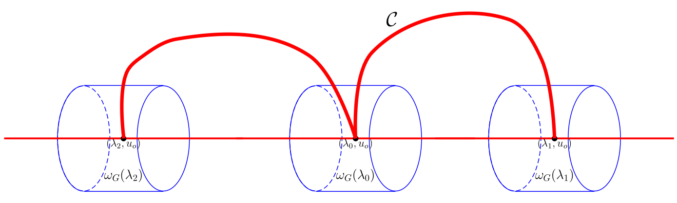
Figure 3: Global bifurcation

By applying formula (4) one can establish an effective criterium allowing to determine the existence of the non-compact branches of nonlinear normal modes with particular (e.g. maximal) orbit types. To be more precise, it is sufficient to consider all the critical frequencies $\lambda_{k}^{-1}$ corresponding to the first Fourier mode and simply show, that for some of them, say $\lambda_{0}^{-1}$, the sum in (4) can never be zero. For the fullerene molecule such non-compact global branches exist.

Novelty.

In this paper, we apply equivariant gradient degree to the classification of the global nonlinear modes in a model of the fullerene molecule $C_{60}$. By taking advantage of various properties of the gradient equivariant degree, the approximate values (obtained numerically) of the normal frequencies can be used to determine (under plausible isotypical non-resonance assumption) the exact values of the topological invariants $\omega_{G}(\lambda_{o})$. In particular, the information contained in the topological invariants can be applied to obtain the presence of such global branches of periodic solutions with the maximal orbit types, as it is presented in our main theorem (Theorem 3.1).

Let us point out that (to the best of our knowledge) all the previous studies of the fullerene molecule have considered only the existence of the linear modes (which have constant frequency), while the occurrence of the non-linear normal modes have frequencies depending on the amplitudes of the oscillation. Such an analysis of nonlinear normal modes for the fullerene molecule was never done before. We complement our results with numerical computations using Newton’s method and pseudo-arclength procedure to continue some of these nonlinear normal modes.

It is important to notice that the icosahedral symmetries appear also in adenoviruses with icosahedral capsid, or other icosahedral molecules considered in [34]. The methods presented here are applicable to these cases as well.

Contents.

The rest of the paper is arranged as follows. In section 2 we present the model equations appropriate for studying the dynamics of the fullerene molecule. In subsection 2.1, we propose a new indexation for the fullerene atoms which greatly simplifies the description of symmetries in the molecule. Then, in subsection 2.2 we discuss the choice of the force field for the fullerene molecule that seems to be the most appropriate in order to model nonlinear vibrations and in subsection 2.3 we describe the action of the group $I\times O(3)$ on the space $\mathscr{V}$. Then, in subsection 2.4, we find the minimizer of the potential $V$ among the configurations with icosahedral symmetries by applying Palais criticality principle. In subsection 2.5, we identify the $I$-isotypical decomposition of the space $\mathscr{V}$ and use it to determine the spectrum of the operator $\nabla^{2}V(u_{o})$ and the $I$-isotypical types of the corresponding eigenspaces. In Section 3 we prove the bifurcation of periodic solutions from the equilibrium configuration $u_{o}$ of the fullerene molecule. In Section 4 we describe the symmetries of the periodic solutions. In addition to the theoretical results stated Theorem 3.1, several of these symmetric periodic solutions were obtained by numerical continuation, for which the numerical data is shown graphically. In Appendix A, we include a short review of the gradient degree, including computational algorithms, and the computations of the $I\times O(2)$-equivariant gradient degree.

2 Fullerene Model

2.1 Equations for Carbons

In this section, we propose a new indexation for the fullerene atoms which greatly simplifies the description of symmetries in the molecule: to each atom we assigned two indices – one (being a $5$-cycle in $S_{5}$) indicating in which the side of the dodecahedron the atom is located and the second indicating its position in that side (as it is illustrated on Figure 1)

Let $A_{5}$ be the alternating group of permutations of five elements $\{1,2,3,4,5\}$. The five conjugacy classes in $A_{5}$ are listed in Table 1. The $C_{60}$ molecule is arranged in $12$ unconnected pentagons of atoms. We implement the following notation for the indices of the $60$ atoms (see Figure 1):

• $\tau\in\mathcal{C}_{4}$ is used to denote each of the $12$ pentagonal faces.

• $k\in\{1,...,5\}=:\mathbb{Z}[1,5]$ is used to denote each of the $5$ vertices in the $12$ pentagonal faces.

$\mathcal{C}_{1}$	$\mathcal{C}_{2}$	$\mathcal{C}_{3}$	$\mathcal{C}_{4}$	$\mathcal{C}_{5}$
$(1)$	$(12)(34)$, $(13)(24)$,$(14)(23)$	$(123)$, $(132)$	$(12345)$	$(12354)$
	$(12)(35)$, $(13)(25)$,$(15)(23)$	$(124)$, $(142)$	$(12453)$	$(12435)$
	$(12)(45)$, $(14)(25)$,$(15)(24)$	$(125)$, $(152)$	$(12534)$	$(12543)$
	$(13)(45)$, $(14)(35)$, $(15)(34)$	$(134)$, $(143)$	$(13254)$	$(13245)$
	$(23)(45)$, $(24)(35)$,$(25)(34)$	$(135)$, $(153)$	$(13542)$	$(13524)$
		$(145)$, $(154)$	$(13425)$	$(13452)$
		$(234)$, $(243)$	$(14235)$	$(14253)$
		$(235)$, $(253)$	$(14352)$	$(14325)$
		$(245)$, $(254)$	$(14523)$	$(14532)$
		$(345)$, $(354)$	$(15243)$	$(15234)$
			$(15432)$	$(15423)$
			$(15324)$	$(15342)$

Table 1: Conjugacy classes of elements in $A_{5}$.

We define the set of indices as

$$\Lambda=\mathcal{C}_{4}\times\mathbb{Z}[1,5]~{}\text{.}$$

With these notations each index $(\tau,k)\in\Lambda$ represents a face and a vertex in the face of the truncated icosahedron as it is shown on Figure 1. The vectors that represent the positions of the carbon atoms are

$$u_{\tau,k}\in\mathbb{R}^{3},$$

and the vector for the $60$ positions is

$$u=(u_{\tau,k})_{(\tau,k)\in\Lambda}\in\left(\mathbb{R}^{3}\right)^{60}\text{.}$$

The space $\left(\mathbb{R}^{3}\right)^{60}$ is a representation of the group $I\times O(3)$, where $I=A_{5}\times\mathbb{Z}_{2}$ stands for the full icosahedral group. With this notation, the action of $I\times O(3)$ on $V$ has a simple definition: the action of $\sigma\in A_{5}$ and $-1\in\mathbb{Z}_{2}$ in $u$ is defined in each component by

$$\rho(\sigma)u_{\tau,k}=u_{\sigma^{-1}\tau\sigma,\sigma^{-1}(k)}~{},\qquad\rho(-1)u_{\tau,k}:=u_{\tau^{-1},k}~{}.$$ (5)

And the action of the group $A\in O(3)$ is defined by

$$Au=(Au_{\tau,k})_{(\tau,k)\in\Lambda}.$$

2.2 Force Field

The system for the fullerene molecule is given by (1). To describe the force field $\nabla V$ we recognize that:

• The $60$ edges in the $12$ pentagonal faces represent single bonds. For these single bonds we define the function $S:\Lambda\rightarrow\Lambda,$

  $$S(\tau,k)=(\tau,\tau(k))~{},\quad\tau\in\mathcal{C}_{4},\;k\in\mathbb{Z}[1,5].$$

• The $30$ remaining edges in the hexagon, which connect the different pentagonal faces, represent double bounds. For these double bonds we define the function $D:\Lambda\rightarrow\Lambda$,

  $$D(\tau,k)=(\sigma,k)\text{ with }\sigma=\left(k,\tau^{2}(k),\tau(k),\tau^{4}(k),\tau^{3}(k)\right).$$

Using the above notation, the force field energy is elegantly expressed by

$$V(u)=\sum_{\left(\tau,k\right)\in\Lambda}\left(U(\left|u_{\tau,k}-u_{S(\tau,k)}\right|)+\frac{1}{2}U(\left|u_{\tau,k}-u_{D(\tau,k)}\right|)+U_{\left(\tau,k\right)}(u)\right)\text{,}$$

where the coefficient $\frac{1}{2}$ before the second term is to eliminate the double count bonds, and the term $U_{\left(\tau,k\right)}(u)$ includes the bending and torsion forces.

Bond stretching is represent by potential

$$U(x)=E_{0}\left(\left(1-e^{-\beta(x-r_{0})}\right)^{2}-1\right),$$

where $r_{0}$ is the equilibrium bond length, $E_{0}$ is the bond energy and $\beta^{-1}$ is the width of the energy. The term $U_{\left(\tau,k\right)}(u)$ includes bending and torsion forces given by

$$U_{\left(\tau,k\right)}(u)=E_{B}(\theta_{1})+E_{B}(\theta_{2})+E_{B}(\theta_{3})+E_{T}(\phi_{1})+E_{T}(\phi_{2})+E_{T}(\phi_{3}),$$

where the bending $E_{B}(\theta)$ around each atom in a molecule is governed by the hybridization of orbitals and is given by

$$E_{B}(\theta)=\frac{1}{2}k_{0}(\cos\theta-\cos\theta_{0})^{2}=\frac{1}{2}k_{\theta}(\cos\theta+1/2)^{2},\quad\theta_{0}:=2\pi/3,$$

(here $\theta_{o}$ is the equilibrium angle and $k_{0}$ is the bending force constant), and the torsion energy $E_{T}(\phi)$ (which describes the energy change associated with rotation around a bond with a four-atom sequence) is given by

$$E_{T}(\phi)=\frac{1}{2}k_{\phi}\left(1-\cos 2\phi\right)=k_{\phi}\left(1-\cos^{2}\phi\right)\text{.}$$

The torsion energy reaches a maximum value at angles $\phi=\pm\pi/2$.

Each carbon $\left(\tau,k\right)\in\Lambda$ has three angles,

$$\cos\theta_{1} =\frac{u_{\tau,k}-u_{S(\tau,k)}}{\left|u_{\tau,k}-u_{S(\tau,k)}\right|}\bullet\frac{u_{\tau,k}-u_{S^{-1}(\tau,k)}}{\left|u_{\tau,k}-u_{S^{-1}(\tau,k)}\right|},$$

$$\cos\theta_{2} =\frac{u_{\tau,k}-u_{D(\tau,k)}}{\left|u_{\tau,k}-u_{D(\tau,k)}\right|}\bullet\frac{u_{\tau,k}-u_{S(\tau,k)}}{\left|u_{\tau,k}-u_{S(\tau,k)}\right|}~{},$$

$$\cos\theta_{3} =\frac{u_{\tau,k}-u_{D(\tau,k)}}{\left|u_{\tau,k}-u_{D(\tau,k)}\right|}\bullet\frac{u_{\tau,k}-u_{S^{-1}(\tau,k)}}{\left|u_{\tau,k}-u_{S^{-1}(\tau,k)}\right|}.$$

Clearly, the bond bending at each atom $\left(\tau,k\right)\in\Lambda$ is $E_{B}(\theta_{1})+E_{B}(\theta_{2})+E_{B}(\theta_{3})$. Let

$$n=\frac{u_{D(\tau,k)}-u_{S(\tau,k)}}{\left|u_{D(\tau,k)}-u_{S(\tau,k)}\right|}\times\frac{u_{D(\tau,k)}-u_{S^{-1}(\tau,k)}}{\left|u_{D(\tau,k)}-u_{S^{-1}(\tau,k)}\right|}$$

be the unit normal vector to the plane passing by $u_{D(\tau,k)}$, $u_{S(\tau,k)}$ and $u_{S^{-1}(\tau,k)}$. Each carbon $\left(\tau,k\right)\in\Lambda$ has three torsion energies given by

$$\cos\phi_{1} =n\bullet n_{1}~{},\qquad n_{1}=\frac{u_{(\tau,k)}-u_{S(\tau,k)}}{\left|u_{(\tau,k)}-u_{S(\tau,k)}\right|}\times\frac{u_{(\tau,k)}-u_{S^{-1}(\tau,k)}}{\left|u_{(\tau,k)}-u_{S^{-1}(\tau,k)}\right|}~{},$$

$$\cos\phi_{2} =n\bullet n_{2}~{},\qquad n_{2}=\frac{u_{(\tau,k)}-u_{D(\tau,k)}}{\left|u_{(\tau,k)}-u_{D(\tau,k)}\right|}\times\frac{u_{(\tau,k)}-u_{S^{-1}(\tau,k)}}{\left|u_{(\tau,k)}-u_{S^{-1}(\tau,k)}\right|}~{},$$

$$\cos\phi_{3} =n\bullet n_{3}~{},\qquad n_{3}=\frac{u_{(\tau,k)}-u_{D(\tau,k)}}{\left|u_{(\tau,k)}-u_{D(\tau,k)}\right|}\times\frac{u_{(\tau,k)}-u_{S(\tau,k)}}{\left|u_{(\tau,k)}-u_{S(\tau,k)}\right|}~{}.$$

Then, the bond bending at each atom $\left(\tau,k\right)\in\Lambda$ is $E_{T}(\phi_{1})+E_{T}(\phi_{2})+E_{T}(\phi_{3})$.

For this work, we use the parameters given in [6] , which are $E_{0}=6.1322~{}eV$, $\beta=1.8502~{}A^{-1}$, $r_{0}=01.4322$ $A$, $k_{\theta}=10~{}eV$, $k_{\phi}=0.346~{}eV$. In this paper we use exactly these values.

2.3 Icosahedral Symmetries

In order to make the system (1) reference point-depended, we define the subspace

$$\mathscr{V}:=\{u\in\left(\mathbb{R}^{3}\right)^{60}:\sum_{(\sigma,k)\in\Lambda}u_{\sigma,k}=0\}$$ (6)

and

$$\Omega_{o}=\left\{u\in\mathscr{V}:u_{\sigma,k}\not=u_{\tau,j}\right\}.$$

We have that $\mathscr{V}$ and $\Omega_{o}$ are flow-invariant for (1)

By the properties of functions $S$ and $D$, the potential

$$V:\Omega_{o}\rightarrow\mathbb{R~{}}$$ (7)

is well defined and $I$-invariant. Moreover, the potential $V$ is invariant by rotations and reflections of the group $O(3)$ because bonding, bending and torsion forces depend only on the norm of the distances among pairs of atoms. Therefore, the potential $V$ is $I\times O(3)$-invariant,

$$V((\sigma,A)u)=V(u),\qquad(\sigma,A)\in I\times O(3)~{}.$$

Let

$$J_{1}:=\left[\begin{array}[c]{ccc}0&0&0\\ 0&0&-1\\ 0&1&0\end{array}\right],\quad J_{2}:=\left[\begin{array}[c]{ccc}0&0&-1\\ 0&0&0\\ 1&0&0\end{array}\right],\quad J_{3}:=\left[\begin{array}[c]{ccc}0&-1&0\\ 1&0&0\\ 0&0&0\end{array}\right]$$ (8)

be the three infinitesimal generators of rotations in $O(3)$, i.e., $e^{\phi J_{1}}$, $e^{\theta J_{2}}$ and $e^{J_{3}\psi}$, where $\phi$, $\theta$ and $\psi$ are the Euler angles. The angle between two adjacent pentagons in a dodecahedron is $\theta_{0}=\arctan 2$. Then, the rotation by $\pi$ that fixes a pair of antipodal edges is

$$A=e^{-\left(\theta_{0}/2\right)J_{2}}e^{\pi J_{3}}e^{\left(\theta_{0}/2\right)J_{2}}=\begin{bmatrix}-\frac{1}{\sqrt{5}}&0&\frac{2}{\sqrt{5}}\\ 0&-1&0\\ \frac{2}{\sqrt{5}}&0&\frac{1}{\sqrt{5}}\end{bmatrix}\text{.}$$ (9)

The rotation by $2\pi/5$ of the upper pentagonal face of a dodecahedron is

$$B=e^{\frac{2\pi}{5}J_{3}}=\begin{bmatrix}\frac{-1+\sqrt{5}}{4}&-\sqrt{\frac{5+\sqrt{5}}{8}}&0\\ \sqrt{\frac{5+\sqrt{5}}{8}}&\frac{-1+\sqrt{5}}{4}&0\\ 0&0&1\end{bmatrix}~{}\text{.}$$ (10)

The subgroup of $O(3)$ generated by the matrices $A$ and $B$ is isomorphic to icosahedral group $A_{5}$. Indeed, the generators $A$ and $B$ satisfy the relations

$$A^{2}=B^{5}=(AB)^{3}=\text{{Id\,}}\ .$$

On the other hand, the group $A_{5}$ is generated by

$$a=(23)(45),\qquad b=\left(12345\right)\text{,}$$ (11)

and we have similar relations

$$a^{2}=b^{5}=(ab)^{3}=(1).$$

Therefore, the explicit homomorphism $\rho:A_{5}\rightarrow\mathrm{SO}(3)$ defined on generators by $\rho(a):=A$ and $\rho(b):=B$ is the required isomorphism $A_{5}\simeq\rho(A_{5})\subset SO(3)$. We extend

$$\rho:A_{5}\times\mathbb{Z}_{2}\rightarrow O(3)$$

with $\rho(-1)=-\text{{Id\,}}\in O(3)$, and consequently we obtain an explicit identification of the full icosahedral group $I$ with $\rho(I)\subset O(3)$.

2.4 Icosahedral Minimizer

Let $\tilde{I}$ be the icosahedral subgroup of $I\times O(3)$ given by

$$\tilde{I}=\left\{(\sigma,\rho(\sigma))\in I\times O(3):\sigma\in I\right\}~{}.$$

The fixed point space

$$\Omega_{0}^{\tilde{I}}=\mathscr{V}^{\tilde{I}}\cap\Omega_{o}=\{\left(a_{\tau,k}\right)_{(\tau,k)\in\Lambda}\in\Omega_{0}:a_{\tau,k}=(\sigma,\rho(\sigma))a_{\tau,k}\},$$

consist of all the truncated icosahedral configurations. An equilibrium of the fullerene molecule can be found as a minimizer of $V$ on these configurations. More precisely, since $V$ is $I\times O(3)$-invariant, by Palais criticality principle, the minimizer of the potential $V$ on the fixed-point space of $\tilde{I}$ is a critical point of $V$.

To find the minimizer among configurations with symmetries $\tilde{I}$, we parameterize the carbons positions by fixing the position of one of them. Let

$$u_{b,1}=(x,0,z),\quad x,z\in\mathbb{R},$$

then we have

$$u_{b,1}=(\sigma,\rho(\sigma))u_{b,1}=\rho(\sigma)u_{\sigma^{-1}b\sigma,\sigma^{-1}(1)}\text{~{},}$$

and relations

$$u_{\sigma^{-1}b\sigma,\sigma^{-1}(1)}=\rho(\sigma)^{-1}u_{b,1}=\rho(\sigma)^{-1}(x,0,z)^{T},\quad\sigma\in A_{5},$$ (12)

allow us to determine the positions of all other coordinates of the vector $u=\left(u_{\tau,k}\right)$.

Therefore, the representation of $u(x,z)$ given by (12) provides us a parametrization of a connected component of $\Omega_{0}^{\tilde{I}}/O(3)$ with the domain

$$\mathcal{D}=\{(x,z)\in\mathbb{R}^{2}:0<z,\;x<Cz\}$$

where $C>0$ is a number determined by the geometric restrictions. We define $v:\mathcal{D}\rightarrow\mathbb{R}$ by

$$v(x,z)=V(u(x,z)).$$

Since $v(x,z)$ is exactly the restriction of $V$ to the fixed-point subspace $\Omega_{0}^{\tilde{I}}/O(3)$, then by the symmetric criticality condition, a critical point of $v:\mathcal{D}\rightarrow\mathbb{R}$ is also a critical point of $V$.

We implemented a numerical minimizing procedure to find the minimizer $(x_{o},z_{o})$ of $v(x,z)$. We denote the truncated icosahedral minimizer corresponding to the fullerene $C_{60}$ as

$$u_{o}=u\left(x_{o},z_{o}\right)\in\mathscr{V}.$$

The lengths of single and double bonds for this minimizer are given by

$$d_{S}=\left|u_{b,1}-u_{S(b,1)}\right|=1.438084,$$

$$d_{D}=\left|u_{b,1}-u_{D(b,1)}\right|=1.420845\text{,}$$

respectively. These results are in accordance with the distances measured in the paper [16].

An advantage of the notation $u=\left(u_{\tau,k}\right)$ is that it is easy to visualize the elements associated to the rotations $\rho(\sigma)$ in the truncated icosahedron (Figure 1). In these configurations we have $\rho(\sigma)u_{\tau,k}=\sigma^{-1}u_{\tau,k}=u_{\sigma\tau\sigma^{-1},\sigma(k)}$, then $\rho(\sigma)$ is identified with the rotation that sends the face $\tau$ to $\sigma\tau\sigma^{-1}$ and the carbon atom identified by $k$ to $\sigma(k)$; for example, under the $\pi$-rotation given by $\rho(a)=A$, face $b=(12345)$ goes to the face $aba^{-1}=(13254)$, and the element $k=1$ to $a(1)=1$. In this manner, we conclude that the elements of the conjugacy classes $\mathcal{C}_{2}$, $\mathcal{C}_{3}$, $\mathcal{C}_{4}$ and $\mathcal{C}_{5}$ correspond to the $15$ rotations by $\pi$, the $20$ rotations by $2\pi/3$, the $12$ rotations by $2\pi/5$ and the $12$ rotations by $\pi/5$, respectively.

2.5 Isotypical Decomposition and Spectrum of $\nabla^{2}V(u_{o})$

The space $\mathscr{V}$ is an orthogonal complement in $\widetilde{\mathscr{V}}=(\mathbb{R}^{3})^{60}$ of the subspace $\{(v,v,\dots,v):v\in\mathbb{R}^{3}\}$, thus it is $\tilde{I}$-invariant. Given that the system (1), $u(t)\in\mathscr{V}$, is symmetric with respect the group action of $I\times O(3)$, the orbit of equilibria $u_{o}$ is a $3$-dimensional submanifold in $\mathscr{V}$. To describe the tangent space, we define

$$\mathcal{J}_{j}u=(J_{j}u_{\sigma,k}),$$

where $J_{j}$ are the three infinitesimal generators of the rotations defined in (8). Then, the slice $S_{o}$ to the orbit of $u_{o}$ is

$$S_{o}:=\{x\in\mathscr{V}:x\bullet\mathcal{J}_{j}u_{0}=0,\quad j=1,2,3\}.$$

Since $u_{o}$ has the isotropy group $\tilde{I}$, then $S_{o}$ is an orthogonal $\tilde{I}$ representation.

In this section we identify the $\tilde{I}$-isotypical components of $S_{o}$. In order to simplify the notation, hereafter we identify $\tilde{I}$ with the group $A_{5}\times\mathbb{Z}_{2}$,

$$\tilde{I}=A_{5}\times\mathbb{Z}_{2}~{}.$$

Put $\varphi_{\pm}=\frac{1}{2}(1\pm\sqrt{5})$, and consider the permutations $a=(2,3)(4,5)$, $b=\left(1,2,3,4,5\right)$ and $c=(1,2,3)$. The character table of $A_{5}$ is:

Rep. Character $$(1)$$

          

The character table of $\tilde{I}\simeq A_{5}\times\mathbb{Z}_{2}$ is obtained from the table of $A_{5}$. We denote the irreducible representations of $I$ by $\mathcal{V}_{\pm n}$ for $n=1,...,5$, where the element $-1\in\mathbb{Z}_{2}$ acts as $\pm\text{{Id\,}}$ in $\mathcal{V}_{\pm n}$ and elements $\gamma\in A_{5}$ act as they act on $\mathcal{V}_{n}$. Notice that all the representations $\mathcal{V}_{\pm n}$ are absolutely irreducible. Therefore, the character table for $A_{5}\times\mathbb{Z}_{2}$ is as follows:

	(1)	$a$	$c$	$b$	$b^{2}$	$(-1)$	$(a,-1)$	$(c,-1)$	$(b,-1)$	$(b^{2},-1)$
$\chi_{1}$	1	1	1	1	1	1	1	1	1	1
$\chi_{2}$	4	0	1	-1	-1	4	0	1	-1	-1
$\chi_{3}$	5	1	-1	0	0	5	1	-1	0	0
$\chi_{4}$	3	-1	0	$\varphi_{+}$	$\varphi_{-}$	3	-1	0	$\varphi_{+}$	$\varphi_{-}$
$\chi_{5}$	3	-1	0	$\varphi_{-}$	$\varphi_{+}$	3	-1	0	$\varphi_{-}$	$\varphi_{+}$
$\chi_{-1}$	1	1	1	1	1	-1	-1	-1	-1	-1
$\chi_{-2}$	4	0	1	-1	-1	-4	0	-1	1	1
$\chi_{-3}$	5	1	-1	0	0	-5	-1	1	0	0
$\chi_{-4}$	3	-1	0	$\varphi_{+}$	$\varphi_{-}$	-3	1	0	$-\varphi_{+}$	$-\varphi_{-}$
$\chi_{-5}$	3	-1	0	$\varphi_{-}$	$\varphi_{+}$	-3	1	0	$-\varphi_{-}$	$-\varphi_{+}$

Table 2: Character table for $A_{5}\times\mathbb{Z}_{2}$

By comparing the character $\chi_{{}_{\mathscr{V}}}$ withe the characters in Table 2, we obtain the following $I$-isotypical decomposition of $\mathscr{V}$

$$\mathscr{V}=\bigoplus_{n=1}^{5}\mathscr{V}_{n}\oplus\mathscr{V}_{-n},$$

where $\mathscr{V}_{\pm n}$ is modeled on $\mathcal{V}_{\pm n}$.

We numerically computed the spectrum $\{\mu_{j}:j=1,2,\dots,47\}$ of the Hessian $\nabla^{2}V(u_{o})$ at this minimizer $u_{o}$. Since $\nabla^{2}V(u_{o}):\mathscr{V}\rightarrow\mathscr{V}$ is $\tilde{I}$-equivariant,

$$\nabla^{2}V(u_{o})|_{\mathscr{V}_{n}\cap E(\mu_{j})}=\mu_{j}\,\text{{Id}}:\mathscr{V}_{n}\cap E(\mu_{j})\rightarrow\mathscr{V}_{n}\cap E(\mu_{j}),$$

where $E(\mu_{j})$ stands for the eigenspace corresponding to $\mu_{j}$. We found that each of the eigenspaces $E(\mu_{j})$ is an irreducible subrepresentation of $\mathscr{V}$ , i.e. the isotypical multiplicity of $\mu_{j}$ is simple. Including the zero eigenspace, we have $47$ different components. Thus we have that $\sigma(\nabla^{2}V(u_{o})|_{{S_{o}}})=\{\mu_{1},...,\mu_{46}\}$ with $\mu_{j}>0$, so

$$S_{o}=\bigoplus_{j=1}^{46}\mathcal{V}_{n_{j}}\quad\text{ and }\quad\nabla^{2}V(u_{o})|_{\mathcal{V}_{n_{j}}}=\mu_{j}\,\text{{Id}.}$$ (13)

In order to determine in which isotypical component $\mathscr{V}_{n_{j}}$ the eigenspace $E(\mu_{j})$ is contained for a given eigenvalue $\mu_{j}$, we apply the isotypical projections

$$P_{{n}}v:=\frac{\dim(\mathcal{V}_{n})}{120}\sum_{g\in\tilde{I}}\chi_{n}(g)~{}gv,\quad v\in\mathscr{V},$$

where $\mathcal{V}_{n}$, $n=\pm 1,\dots,\pm 5$, is the irreducible representation identified by the character Table 2. Then the component $\mathscr{V}_{n_{j}}$ can be clearly identified by the projection $P_{n_{j}}$.

$j$	Mult.	$\mu_{j}$	$\lambda_{j}$	${\small n}_{j}$
1	5	176.536	$0.075263$	-3
2	5	176.366	$0.075300$	3
3	4	164.083	$0.078067$	2
4	4	160.292	$0.078985$	-2
5	3	159.290	$0.079233$	-5
6	5	148.597	$0.082034$	3
7	3	141.071	$0.084194$	-4
8	3	140.573	$0.084343$	5
9	1	135.632	$0.085866$	1
10	4	134.935	$0.086087$	-2
11	4	129.544	$0.087860$	2
12	5	125.431	$0.089289$	-3
13	3	107.719	$0.096350$	4
14	5	98.5525	$0.100732$	3
15	3	93.4648	$0.103437$	-5
16	5	87.7541	$0.106750$	-3
17	3	83.9718	$0.109127$	-4
18	4	71.6288	$0.118156$	2
19	5	67.1181	$0.122062$	3
20	1	59.3865	$0.129765$	-1
21	3	50.4797	$0.140748$	-5
22	4	47.5646	$0.144997$	-2
23	3	42.2947	$0.153765$	4

$j$	Mult.	${\small\mu}_{j}$	$\lambda_{j}$	$n_{j}$
24	3	41.3918	$0.155433$	5
25	4	33.9885	$0.171528$	-2
26	5	28.8031	$0.186329$	-3
27	5	27.4795	$0.190764$	3
28	3	27.3153	$0.191336$	5
29	4	25.5388	$0.197879$	-2
30	4	22.7212	$0.209790$	2
31	5	19.4536	$0.226725$	-3
32	5	19.3377	$0.227404$	3
33	3	19.2379	$0.227993$	-5
34	4	16.5356	$0.245918$	2
35	3	16.5255	$0.245993$	5
36	3	15.1033	$0.257314$	-4
37	3	10.3908	$0.310224$	4
38	1	10.2520	$0.312317$	1
39	5	10.1098	$0.314506$	-3
40	3	9.03077	$0.332765$	-4
41	4	9.02666	$0.332841$	2
42	5	6.99929	$0.377984$	3
43	5	6.95354	$0.379225$	-3
44	3	5.42311	$0.429414$	-5
45	4	5.26429	$0.435843$	-2
46	5	3.04384	$0.573177$	3

Table 3: Eigenvalues $\mu_{j}$ of $\nabla^{2}V(u_{o})$ and critical numbers $\lambda_{j}$ according to their isotypical type $\mathcal{V}_{n_{j}}$.

In the following Table 3, we show the number $n_{j}\in\{-5,...,-1,1,...,5\}$ that identifies the irreducible representation corresponding to the eigenvalue $\mu_{j}$ for $j=1,..,46$. The numerical computations strongly indicate that all the eigenvalues $\mu_{j}$, $j=1,..,46$, are non-resonant.

Remark 2.1.

The models proposed in [33] and [6], consider the presence of van der Waals forces among carbon atoms, which are modeled by the potential

$$W(x)=\varepsilon\left(\frac{\sigma^{12}}{x^{12}}-2\frac{\sigma^{6}}{x^{6}}\right)~{},$$

where $\sigma=3.4681~{}A^{-1}$ is the minimum energy distance and $\epsilon=0.0115~{}eV$ the depth of this minimum. Our numerical computations indicate that the models with van der Waals forces do not produce acceptable bond lengths between the atoms (as it is given in [16]), neither the spectrums fit the experimental data (cf. [8]). Actually, the models [33] and [6] without van der Waals forces lead to results which correctly approximate the measurements in [16] and [8] (for bond lengths $d_{S}$ and $d_{D}$ and frequencies $\sqrt{\mu_{j}/m}$, which are within the range $100$ to $1800$ $cm^{-1}$).

3 Equivariant Bifurcation

In what follows, we are interested in finding non-trivial $T$-periodic solutions to (1), bifurcating from the $G$-orbit of the equilibrium point $u_{o}$. By normalizing the period, i.e. by making the substitution $v(t):=u\left(\lambda t\right)$ in (1), we obtain the system

$$\begin{cases}\ddot{v}=-\lambda^{2}\nabla V(v),\\ v(0)=v(2\pi),\;\;\dot{v}(0)=\dot{v}(2\pi),\end{cases}$$ (14)

where $\lambda^{-1}=2\pi/T$ is the frequency.

3.1 Equivariant Gradient Map

Since $\mathscr{V}$ is an orthogonal $I\times O(3)$- representation, we can consider the first Sobolev space of $2\pi$-periodic functions from $\mathbb{R}$ to $\mathscr{V}$, i.e.,

$$H_{2\pi}^{1}(\mathbb{R},\mathscr{V}):=\{u:\mathbb{R}\rightarrow\mathscr{V}\;:\;u(0)=u(2\pi),\;u|_{[0,2\pi]}\in H^{1}([0,2\pi];\mathscr{V})\},$$

equipped with the inner product

$$\langle u,v\rangle:=\int_{0}^{2\pi}(\dot{u}(t)\bullet\dot{v}(t)+u(t)\bullet v(t))dt~{}.$$

Let $O(2)=SO(2)\cup\kappa SO(2)$ denote the group of $2\times 2$-orthogonal matrices, where

$$\kappa=\left[\begin{array}[c]{cc}1&0\\ 0&-1\end{array}\right],\qquad\left[\begin{array}[c]{cc}\cos\tau&-\sin\tau\\ \sin\tau&\cos\tau\end{array}\right]\in SO(2)~{}.$$

It is convenient to identify a rotation with $e^{i\tau}\in S^{1}\subset\mathbb{C}$. Notice that $\kappa e^{i\tau}=e^{-i\tau}\kappa$, i.e., $\kappa$ as a linear transformation of $\mathbb{C}$ into itself, acts as complex conjugation.

Clearly, the space $H_{2\pi}^{1}(\mathbb{R},\mathscr{V})$ is an orthogonal Hilbert representation of

$$G:=I\times O(3)\times O(2).$$

Indeed, we have for $u\in H_{2\pi}^{1}(\mathbb{R},\mathscr{V})$ and $(\sigma,A)\in I\times O(3)$ (see (5))

$$\left(\sigma,A\right)u(t) =(\sigma,A)u(t),$$ (15)

$$e^{i\tau}u(t) =u(t+\tau),$$

$$\kappa u(t) =u(-t).$$

It is useful to identify a $2\pi$-periodic function $u:\mathbb{R}\rightarrow V$ with a function $\widetilde{u}:S^{1}\rightarrow\mathscr{V}$ via the map $\mathfrak{e}(\tau)=e^{i\tau}:\mathbb{R}$$\rightarrow S^{1}$. Using this identification, we will write $H^{1}(S^{1},\mathscr{V})$ instead of $H_{2\pi}^{1}(\mathbb{R},\mathscr{V})$. Let

$$\Omega:=\{u\in H^{1}(S^{1},\mathscr{V}):u(t)\in\Omega_{o}\}.$$

We define $J:\mathbb{R}\times\Omega\rightarrow\mathbb{R}$ by

$$J(\lambda,u):=\int_{0}^{2\pi}\left[\frac{1}{2}|\dot{u}(t)|^{2}-\lambda^{2}V(u(t))\right]dt.$$ (16)

Then, the system (14) can be written as the following variational equation

$$\nabla_{u}J(\lambda,u)=0,\quad(\lambda,u)\in\mathbb{R}\times\Omega.$$ (17)

Consider $u_{o}\in\mathscr{V}$ – the equilibrium point of (7) (i.e. symmetric ground state) described in previous section. Then $u_{o}$ is a critical point of $J$. We are interested in finding non-stationary $2\pi$-periodic solutions bifurcating from $u_{o}$, i.e. non-constant solutions to system (17). We consider the orbit $G(u_{o})$ of $u_{o}$ in $H^{1}(S^{1},\mathscr{V})$. We denote by $\mathcal{S}_{o}$ the slice to $G(u_{o})$ in $H^{1}(S^{1},\mathscr{V})$. We consider the $G_{u_{o}}$-invariant restriction $J:\mathbb{R}\times\left(\mathcal{S}_{o}\cap\Omega\right)\rightarrow\mathbb{R}$ of $J$ to the set $\mathcal{S}_{o}\cap\Omega$. This restriction will allow us to apply the Slice Criticality Principle (see Theorem A.2) in order to compute the gradient equivariant degree of $\nabla J_{\lambda}$ on a small neighborhood $\mathscr{U}$ of $G(u_{o})$ needed for evaluation of the equivariant invariant $\omega_{G}(\lambda)$.

Consider the operator $L:H^{2}(S^{1};\mathscr{V})\rightarrow L^{2}(S^{1};\mathscr{V})$, given by

$$Lu=-\ddot{u}+u$$

for $u\in H^{2}(S^{1},\mathscr{V})$. Then the inverse operator $L^{-1}$ exists and is bounded. Let $j:H^{2}(S^{1};\mathscr{V})\rightarrow H^{1}(S^{1},\mathscr{V})$ be the natural embedding operator. Clearly, $j$ is a compact operator. Then, one can easily verify that

$$\nabla_{u}J(\lambda,u)=u-j\circ L^{-1}(\lambda^{2}\nabla V(u)+u),$$ (18)

where $u\in H^{1}(S^{1},\mathscr{V})$. Consequently, the bifurcation problem (17) is equivalent to $\nabla_{u}J(\lambda,u)=0$. Moreover, we have

$$\nabla_{u}^{2}J(\lambda,u_{o})v=v-j\circ L^{-1}(\lambda^{2}\nabla^{2}V(u_{o})v+v)~{},$$ (19)

where $v\in H^{1}(S^{1},\mathscr{V})$.

Notice that

$$\mathscr{A}(\lambda):=\nabla_{u}^{2}J(\lambda,u_{o})|_{\mathcal{S}_{o}}:\mathcal{S}_{o}\rightarrow\mathcal{S}_{o}.$$

Thus, by implicit function theorem, $G(u_{o})$ is an isolated orbit of critical points, whenever $\mathscr{A}(\lambda)$ is an isomorphism. Therefore, if a point $(\lambda_{o},u_{o})$ is a bifurcation point for (17), then $\mathscr{A}(\lambda_{o})$ cannot be an isomorphism. In such case we define

$$\Lambda:=\{\lambda>0:\mathscr{A}(\lambda_{o})\text{ is not an isomorphism}\}~{},$$

and call this set the critical set for the trivial solution $u_{o}$.

3.2 Critical Numbers

Consider the $S^{1}$-action on $H^{1}(S^{1},\mathscr{V})$, where $S^{1}$ acts on functions by shifting the argument (see (15)). Then, $(H^{1}(S^{1},\mathscr{V}))^{S^{1}}$ is the space of constant functions, which can be identified with the space $\mathscr{V}$, i.e.,

$$H^{1}(S^{1},\mathscr{V})=\mathscr{V}\oplus\mathscr{W},\quad\mathscr{W}:=\mathscr{V}^{\perp}.$$

Then, the slice $\mathcal{S}_{o}$ in $H^{1}(S^{1},\mathscr{V})$ to the orbit $G(u_{o})$ at $u_{o}$ is exactly

$$\mathcal{S}_{o}=S_{o}\oplus\mathscr{W}.$$

Consider the $S^{1}$-isotypical decomposition of $\mathscr{W}$, i.e.,

$$\mathscr{W}=\overline{\bigoplus_{l=1}^{\infty}\mathscr{W}_{l}},\quad\mathscr{W}_{l}:=\{\cos(l\cdot)\mathfrak{a}+\sin(l\cdot)\mathfrak{b}:\mathfrak{a},\,\mathfrak{b}\in\mathscr{V}\}$$

In a standard way, the space $\mathscr{W}_{l}$, $l=1,2,\dots$, can be naturally identified with the complexification $\mathscr{V}^{\mathbb{C}}$ on which $S^{1}$ acts by $l$-folding,

$$\mathscr{W}_{l}=\{e^{il\cdot}z:z\in\mathscr{V}^{\mathbb{C}}\}.$$

Since the operator $\mathscr{A}(\lambda)$ is $G_{u_{o}}$-equivariant with

$$G_{u_{o}}=\tilde{I}\times O(2),$$

it is also $S^{1}$-equivariant and thus $\mathscr{A}(\lambda)(\mathscr{W}_{l})\subset\mathscr{W}_{l}$. Using the $\tilde{I}$-isotypical decomposition of $\mathscr{V}^{\mathbb{C}}$, we have the $G_{u_{o}}$-invariant decomposition

$$\mathscr{W}_{l}=\bigoplus_{j=1}^{46}\mathcal{V}_{{j},l},\quad\mathcal{V}_{{j},l}:=\{e^{il\cdot}z:z\in E(\mu_{j})^{\mathbb{C}}\},$$

where $\mathcal{V}_{n_{j},l}=\mathcal{V}_{n_{j}}^{\mathbb{C}}=\mathbb{C}\otimes_{\mathbb{R}}\mathcal{V}_{n_{j}}$ is the $I\times O(2)$-irreducible representation with $O(2)$ acting on $\mathbb{C}$ by $l$-folding and complex conjugation. We have

$$\mathscr{A}(\lambda)|_{\mathcal{V}_{{j},l}}=\left(1-\frac{\lambda^{2}\mu_{j}+1}{l^{2}+1}\right)\text{\rm Id\,}.$$

Thus $A(\lambda_{o})|_{\mathcal{V}_{{j},l}}=0$ if and only if $\lambda_{o}^{2}=l^{2}/\mu_{j}$ for some $l=1,2,3,\dots$ and $j=0,1,2,\dots,46$.

We will write

$$\lambda_{j,l}=\frac{l}{\sqrt{\mu_{j}}}$$

to denote the critical numbers in $\Lambda$. Then the critical set for the equilibrium $u_{o}$ of system (7) is

$$\Lambda=\{\lambda_{j,l}:j=0,...,46,\quad l=1,2,3,\dots\}.$$

Let us point out that in the case of isotypical resonances, the critical numbers may not be uniquely identified by indices $(j,l)$. The first and last critical numbers for $l=1$ are $\lambda_{1,1}=.07526\,3$ and $\lambda_{46,1}=0.573\,18$, respectively. We computed numerically (with precision $10^{-5}$) all the different values $\lambda_{j,l}$ from $\lambda_{1,1}$ to $\lambda_{46,1}$. We obtain that among these approximations there is no-resonance with harmonic critical number from $\lambda_{1,1}$ to $\lambda_{46,1}$, i.e.,

$$\lambda_{1,1}<\lambda_{2,1}<\lambda_{3,1}<\lambda_{4,1}<...<\lambda_{5,7}<\ \lambda_{26,3}<\lambda_{21,4}<\lambda_{27,3}<\lambda_{46,1}.$$ (20)

Therefore, a plausible assumption under the numerical evidence is that all the eigenvalues $\lambda_{j,1}$ are isotypical non-resonant for $j=1,...,46$.

3.3 Conjugacy Classes of Subgroups in $I\times O(2)$

In order to simplify the notation, in what follows, instead of using the symbol $\tilde{I}$, we will write $I$. Under this notation the isotropy group $G_{u_{o}}$ is

$$G_{u_{o}}=I\times O(2).$$

The notation in this section is useful to obtain the classification of all conjugacy classes $(\mathscr{H})$ of closed subgroups in $I\times O(2)$.

The representatives of the conjugacy classes of the subgroups in $A_{5}\times\mathbb{Z}_{2}$ consisting of proper nontrivial subgroups of $A_{5}$ are:

$$\mathbb{Z}_{2} =\{((1),1),\,((12)(34),1)\},$$

$$\mathbb{Z}_{3} =\{((1),1)\,,((123),1),\,((132),1)\},$$

$$V_{4} =\{((1),1),\,((12)(34),1),\,((13)(24),1),\,((23)(14),1)\},$$

$$\mathbb{Z}_{5} =\{((1),1),\,((12345),1),\,((13524),1),\,((14253),1),\,((15432),1)\},$$

$$D_{3} =\{((1),1),\,((123),1),\,((132),1),\,((12)(45),1),\,((13)(45),1),\,((23)(45),1)\},$$

$$A_{4} =\{((1),1),\,((12)(34),1),\,((13)(24),1),\,((14)(23),1),\,((123),1),\,((132),1),\,((124),1),$$

$$\hskip 14.22636pt((142),1,\,((134),1),\,((143),1),\,((234),1),\,((243),1)\},$$

$$D_{5} =\{((1),1),\,((12345),1),\,((13524),1),\,((14253),1),\,((15432),1),\,((12)(35),1),\,((13)(45),1),$$

$$\hskip 14.22636pt((14)(23),1),\,((15)(24),1),\,((25)(34)\}.$$

The representatives of the additional conjugacy classes of the subgroups in $A_{5}\times\mathbb{Z}_{2}$ will be used to describe the symmetries of nonlinear vibrations. Besides of the product subgroups $H^{p}:=H\times\mathbb{Z}_{2}$, we have the also following twisted subgroups $H^{\varphi}$ of $A_{5}\times\mathbb{Z}_{2}$ (where $H$ is a subgroup of $A_{5}$):

$$\mathbb{Z}_{2}^{z} =\Big{\{}\big{(}(1),1\big{)},\,\big{(}(12)(34),-1\big{)}\Big{\}},$$

$$V_{4}^{z} =\Big{\{}\big{(}(1),1\big{)},\,\big{(}(12)(34),-1\big{)},\,\big{(}(13)(24),-1\big{)},\,\big{(}(23)(14),1\big{)}\Big{\}},$$

$$D_{3}^{z} =\Big{\{}\big{(}(1),1\big{)},\,\big{(}(123),1\big{)},\,\big{(}(132),1\big{)},\,\big{(}(12)(45),-1\big{)},\,\big{(}(13)(45),-1\big{)},$$

$$\hskip 14.22636pt\,\big{(}(23)(45),-1\big{)}\Big{\}},$$

$$D_{5}^{z} =\Big{\{}\big{(}(1),1\big{)},\,\big{(}(12345),1\big{)},\,\big{(}(13524),1\big{)},\,\big{(}14253),1\big{)},\,\big{(}(15432),1\big{)},$$

$$\hskip 14.22636pt\,\big{(}(12)(35),-1\big{)},\,\big{(}(13)(45),-1\big{)},\,\big{(}(14)(23),-1\big{)},\,\big{(}(15)(24),-1\big{)},$$

$$\hskip 14.22636pt\,\big{(}(25)(34),-1\big{)}\Big{\}}.$$

With these definitions the subconjugacy lattice for $A_{5}\times\mathbb{Z}_{2}$ is shown in Figure 4.

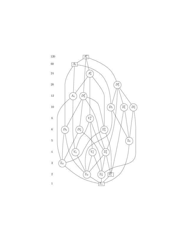
Figure 4: Lattice of conjugacy classes of subgroups in $A_{5}\times\mathbb{Z}_{2}$. The square boxes indicate that the related subgroup is normal in $A_{5}\times\mathbb{Z}_{2}$.

The result (see [9, 15]) provides a description of subgroups of the product group $I\times O(2)$. Namely, for any subgroup $\mathscr{H}$ of the product group $I\times O(2)$, there exist subgroups $H\leq I$ and $K\leq O(2)$, a group $L$ and two epimorphisms $\varphi:H\rightarrow L$ and $\psi:K\rightarrow L$ such that

$$\mathscr{H}=\{(h,k)\in H\times K:\varphi(h)=\psi(k)\}.$$

In order to make the notation self-contained, we will assume that $L=K/\ker(\psi)$, so $\psi:K\rightarrow L$ is evidently the natural projection. On the other hand, the group $L$ can be naturally identified with a finite subgroup of $O(2)$ being either $D_{n}$ or $\mathbb{Z}_{n}$. Since we are interested in describing conjugacy classes of $\mathscr{H}$, we can identify different epimorphisms $\varphi,\psi:H\rightarrow L$ by indicating

$$Z=\text{Ker\thinspace}(\varphi)\quad\text{ and }\quad L=K/\ker(\psi).$$

Therefore, to identify $\mathscr{H}$ we will write

$$\mathscr{H}=:H{\prescript{Z}{}{\times}_{L}^{m}}K~{},$$ (21)

where $H$ and $Z$ are subgroups of $I$ and $m$ is a number used to identify groups in different conjugacy classes. In the case that all the epimorphisms $\varphi$ with the kernel $Z$ are conjugate, there is no need to use the number $m$ in (21), so we will simply write $\mathscr{H}=H{\prescript{Z}{}{\times}_{L}K}$. In addition, in the case that all epimorphisms $\varphi$ from $H$ to $L$ are conjugate, we can also omit the symbol $Z$, i.e. we will write $\mathscr{H}=H\times_{L}K$.

3.4 Bifurcation Theorem

Theorem 3.1.

Assume that the critical numbers $\lambda_{j,1}\in\Lambda$, $j=1,2,\dots,46$, for the system (17) are isotypically non-resonant. Then, there exist multiple global bifurcations of solutions from the critical number $\lambda_{j,1}$ corresponding to the irreducible representation $V_{n_{j}}$ in Table 3:

• For $n_{j}=1$ there exists a $G$-orbit of a branch of periodic solutions with the orbit type ${({A_{5}^{p}}\prescript{}{}{\times}D_{1})}$;

• For $n_{j}=2$ there exist $G$-orbits of branches of periodic solutions with the orbit types ${({D_{3}^{p}}\prescript{{\mathbb{Z}_{3}^{p}}}{}{\times}_{\mathbb{Z}_{2}}D_{2})}$, ${({V_{4}^{p}}\prescript{{\mathbb{Z}_{2}^{p}}}{}{\times}_{\mathbb{Z}_{2}}D_{2})}$, ${({A_{4}^{p}}\prescript{}{}{\times}D_{1})}$, ${({D_{3}^{p}}\prescript{}{}{\times}D_{1})}$, ${({D_{5}^{p}}\prescript{{\mathbb{Z}_{1}^{p}}}{}{\times}^{{1}}_{D_{5}}D_{5})}$, ${({D_{5}^{p}}\prescript{{\mathbb{Z}_{1}^{p}}}{}{\times}^{{2}}_{D_{5}}D_{5})}$, ${({D_{3}^{p}}\prescript{{\mathbb{Z}_{1}^{p}}}{}{\times}_{D_{3}}D_{3})}$;

• For $n_{j}=3$ there exist $G$-orbits of branches of periodic solutions with the orbit types ${({V_{4}^{p}}\prescript{{\mathbb{Z}_{2}^{p}}}{}{\times}_{\mathbb{Z}_{2}}D_{2})}$, ${({D_{5}^{p}}\prescript{}{}{\times}D_{1})}$, ${({D_{3}^{p}}\prescript{}{}{\times}D_{1})}$, ${({D_{5}^{p}}\prescript{{\mathbb{Z}_{1}^{p}}}{}{\times}^{{1}}_{D_{5}}D_{5})}$, ${({D_{5}^{p}}\prescript{{\mathbb{Z}_{1}^{p}}}{}{\times}^{{2}}_{D_{5}}D_{5})}$, ${(A_{4}^{p}\prescript{V_{4}^{p}}{}{\times}_{\mathbb{Z}_{3}}\mathbb{Z}_{3})}$;

• For $n_{j}=4$ there exist $G$-orbits of branches of periodic solutions with the orbit types ${({D_{5}^{p}}\prescript{{\mathbb{Z}_{5}^{p}}}{}{\times}_{\mathbb{Z}_{2}}D_{2})}$, ${({D_{3}^{p}}\prescript{{\mathbb{Z}_{3}^{p}}}{}{\times}_{\mathbb{Z}_{2}}D_{2})}$, ${({V_{4}^{p}}\prescript{{\mathbb{Z}_{2}^{p}}}{}{\times}_{\mathbb{Z}_{2}}D_{2})}$, ${({D_{5}^{p}}\prescript{{\mathbb{Z}_{1}^{p}}}{}{\times}^{{1}}_{D_{5}}D_{5})}$, ${({D_{3}^{p}}\prescript{{\mathbb{Z}_{1}^{p}}}{}{\times}_{D_{3}}D_{3})}$,

• For $n_{j}=5$ there exist $G$-orbits of branches of periodic solutions with the orbit types ${({D_{5}^{p}}\prescript{{\mathbb{Z}_{5}^{p}}}{}{\times}_{\mathbb{Z}_{2}}D_{2})}$, ${({D_{3}^{p}}\prescript{{\mathbb{Z}_{3}^{p}}}{}{\times}_{\mathbb{Z}_{2}}D_{2})}$, ${({V_{4}^{p}}\prescript{{\mathbb{Z}_{2}^{p}}}{}{\times}_{\mathbb{Z}_{2}}D_{2})}$, ${({D_{5}^{p}}\prescript{{\mathbb{Z}_{1}^{p}}}{}{\times}^{{2}}_{D_{5}}D_{5})}$, ${({D_{3}^{p}}\prescript{{\mathbb{Z}_{1}^{p}}}{}{\times}_{D_{3}}D_{3})}$;

• For $n_{j}=-1$ here exists a $G$-orbit of a branch of periodic solutions with the orbit type ${({A_{5}^{p}}\prescript{{A_{5}}}{}{\times}_{\mathbb{Z}_{2}}D_{2})}$;

• For $n_{j}=-2$ there exist $G$-orbits of branches of periodic solutions with the orbit types ${({A_{4}^{p}}\prescript{{A_{4}}}{}{\times}_{\mathbb{Z}_{2}}D_{2})}$, ${({D_{3}^{p}}\prescript{{D_{3}^{z}}}{}{\times}_{\mathbb{Z}_{2}}D_{2})}$, ${({D_{3}^{p}}\prescript{{D_{3}}}{}{\times}_{\mathbb{Z}_{2}}D_{2})}$,${({V_{4}^{p}}\prescript{{V_{4}^{z}}}{}{\times}_{\mathbb{Z}_{2}}D_{2})}$, ${({D_{5}^{p}}\prescript{{\mathbb{Z}_{1}}}{}{\times}^{{1}}_{D_{10}}D_{10})}$, ${({D_{5}^{p}}\prescript{{\mathbb{Z}_{1}}}{}{\times}^{{2}}_{D_{10}}D_{10})}$, ${({D_{3}^{p}}\prescript{{\mathbb{Z}_{1}}}{}{\times}_{D_{6}}D_{6})}$,

• For $n_{j}=-3$ there exist $G$-orbits of branches of periodic solutions with the orbit types ${({D_{5}^{p}}\prescript{{D_{5}}}{}{\times}_{\mathbb{Z}_{2}}D_{2})}$, ${({D_{3}^{p}}\prescript{{D_{3}}}{}{\times}_{\mathbb{Z}_{2}}D_{2})}$, ${({V_{4}^{p}}\prescript{{V_{4}^{z}}}{}{\times}_{\mathbb{Z}_{2}}D_{2})}$,${({D_{5}^{p}}\prescript{{\mathbb{Z}_{1}}}{}{\times}^{{1}}_{D_{10}}D_{10})}$, ${({D_{5}^{p}}\prescript{{\mathbb{Z}_{1}}}{}{\times}^{{2}}_{D_{10}}D_{10})}$, ${(A_{4}^{p}\prescript{V_{4}}{}{\times}_{\mathbb{Z}_{6}}\mathbb{Z}_{6})}$;

• For $n_{j}=-4$ there exist $G$-orbits of branches of periodic solutions with the orbit types ${({D_{5}^{p}}\prescript{{D_{5}^{z}}}{}{\times}_{\mathbb{Z}_{2}}D_{2})}$, ${({D_{3}^{p}}\prescript{{D_{3}^{z}}}{}{\times}_{\mathbb{Z}_{2}}D_{2})}$, ${({V_{4}^{p}}\prescript{{V_{4}^{z}}}{}{\times}_{\mathbb{Z}_{2}}D_{2})}$,${({D_{5}^{p}}\prescript{{\mathbb{Z}_{1}}}{}{\times}^{{1}}_{D_{10}}D_{10})}$, ${({D_{3}^{p}}\prescript{{\mathbb{Z}_{1}}}{}{\times}_{D_{6}}D_{6})}$;

• For $n_{j}=-5$ there exist $G$-orbits of branches of periodic solutions with the orbit types ${({D_{5}^{p}}\prescript{{D_{5}^{z}}}{}{\times}_{\mathbb{Z}_{2}}D_{2})}$, ${({D_{3}^{p}}\prescript{{D_{3}^{z}}}{}{\times}_{\mathbb{Z}_{2}}D_{2})}$, ${({V_{4}^{p}}\prescript{{V_{4}^{z}}}{}{\times}_{\mathbb{Z}_{2}}D_{2})}$,${({D_{5}^{p}}\prescript{{\mathbb{Z}_{1}}}{}{\times}^{{2}}_{D_{10}}D_{10})}$, ${({D_{3}^{p}}\prescript{{\mathbb{Z}_{1}}}{}{\times}_{D_{6}}D_{6})}$.

Proof.

The critical numbers for system (17) are $\lambda_{j,l}=l/\sqrt{\mu_{j}}$ for $l=1,2,3,\dots,$ and $j=1,2,\dots,46$, where $\mu_{j}$ (together with its isotypical types) are listed in Table 3. We assumed (under the numerical evidence) that the critical frequencies $\lambda_{j,1}^{-1}$ are isotypically non-resonant. Based on the ideas explained in section 1, then $\lambda_{o}:=\lambda_{j_{o},1}$ is an isolated critical point in $\Lambda$. That is, there are $\lambda_{-}<\lambda_{o}<\lambda_{+}$ such that $[\lambda_{-},\lambda_{+}]\cap\Lambda=\{\lambda_{o}\}$. Moreover, there exists an isolating $G$-neighborhood $\mathscr{U}$ of $G(u_{o})$ such that no other critical orbits of $J_{\lambda_{\pm}}$ belong to $\overline{\mathscr{U}}$. Thus, we can define the topological invariant $\omega_{G}(\lambda_{o})$ by (3). Then, by the properties of the gradient equivariant degree, if

$$\omega_{G}(\lambda_{o})=n_{1}(H_{1})+n_{2}(H_{2})+\dots+n_{m}(H_{m})$$

is non-zero, i.e. $n_{j}\not=0$ for a $j=1,2,\dots,m$, then there exists a bifurcating branch of nontrivial solutions to (17) from the orbit $\{\lambda_{o}\}\times G(u_{o})$ with symmetries at least $(H_{j})$.

Next, by Theorem A.2,

$$\nabla_{G}\text{-deg}(\nabla J_{\lambda_{\pm}},\mathscr{U})=\Theta\left(\nabla_{G_{u_{o}}}\text{-deg}(\nabla{J}_{\lambda_{\pm}},\mathscr{U}\cap\mathscr{S}_{o})\right),$$

where $G=I\times O(3)\times O(2)$, $G_{u_{o}}=\tilde{I}\times O(2)$ and $\Theta:U(G_{u_{o}})\rightarrow U(G)$ is the homomorfism given by $\Theta(H)=(H)$. For convenience, in what follows we will ignore the symbol $\Theta$. Moreover, by standard linearization technique, we have

$$\nabla_{G_{u_{o}}}\text{-deg}(\nabla{J}_{\lambda_{\pm}},\mathscr{U}\cap\mathscr{S}_{o})=\nabla_{G_{u_{o}}}\text{-deg}(\mathscr{A}_{\lambda_{\pm}},\mathscr{U}\cap\mathscr{S}_{o}).$$

By (34), since all the eigenvalues $\mu_{j}$ are isotopically simple, we have

$$\nabla_{G_{u_{o}}}\text{-deg}(\mathscr{A}_{\lambda_{-}},\mathscr{U}\cap\mathscr{S}_{o}) =\prod_{\left\{\left(j,l\right)\in\mathbb{N}^{2}:\lambda_{j,l}<\lambda_{o}\right\}}\nabla\text{-deg}_{\mathcal{V}_{n_{j},l}},$$

$$\nabla_{G_{u_{o}}}\text{-deg}(\mathscr{A}_{\lambda_{+}},\mathscr{U}\cap\mathscr{S}_{o}) =\nabla\text{-deg}_{\mathcal{V}_{n_{j_{o}},l}}\prod_{\left\{\left(j,l\right)\in\mathbb{N}^{2}:\lambda_{j,l}<\lambda_{o}\right\}}\nabla\text{-deg}_{\mathcal{V}_{n_{j},l}},$$

where $\nabla\text{-deg}_{\mathcal{V}_{n_{j},l}}$ are gradient $I\times O(2)$-equivariant basic degrees listed in Appendix A.6. Therefore, we obtain

$$\omega_{G}(\lambda_{o}):=\Big{(}(I\times O(2))-\nabla\text{-deg}_{\mathcal{V}_{n_{j_{o}},1}}\Big{)}\prod_{\left\{\left(j,l\right)\in\mathbb{N}^{2}:\lambda_{j,l}<\lambda_{o}\right\}}\nabla\text{-deg}_{\mathcal{V}_{n_{j},l}},$$

where $(I\times O(2))$ is the unit element in $U(I\times O(2))$. For instance, the first equivariant invariants are given by

$$\omega_{G}(\lambda_{1,1}) =(I\times O(2))-\nabla\text{-deg}_{\mathcal{V}_{3,1}}$$

$$\omega_{G}(\lambda_{2,1}) =\nabla\text{-deg}_{\mathcal{V}_{3,1}}\ast\Big{(}(I\times O(2))-\nabla\text{-deg}_{\mathcal{V}_{-3,1}}\Big{)}$$

$$\omega_{G}(\lambda_{3,1}) =\nabla\text{-deg}_{\mathcal{V}_{3,1}}\ast\nabla\text{-deg}_{\mathcal{V}_{-3,1}}\ast\Big{(}(I\times O(2))-\nabla\text{-deg}_{\mathcal{V}_{2,1}}\Big{)}.$$

We will prove that a maximal orbit type $(H)$ that appears in the gradient $I\times O(2)$-basic degree $\nabla\text{-deg}_{\mathcal{V}_{n_{j_{o}},1}}$ with non-zero coefficient $n_{H}$,

$$\nabla\text{-deg}_{\mathcal{V}_{n_{j_{o}},1}}=(I\times O(2))+n_{H}(H)+\dots,$$

also appears in $\omega_{G}(\lambda_{o})$ with non-zero coefficients. Hereafter, dots indicate all the remaining terms corresponding to orbit types strictly smaller than $(H)$. Notice that all such maximal orbit types (which are indicated in subsection A.6 by red color) belong to $\Phi_{0}(I\times O(2))$ (i.e. dim $W(H)=0$) except for $(A_{4}^{p}\prescript{V_{4}^{p}}{}{\times}_{\mathbb{Z}_{3}}\mathbb{Z}_{3})$ (in $\nabla\text{-deg}_{\mathcal{V}_{3,1}}$) and $(A_{4}^{p}\prescript{V_{4}}{}{\times}_{\mathbb{Z}_{6}}\mathbb{Z}_{6}))$ (in $\nabla\text{-deg}_{\mathcal{V}_{-3,1}}$).

Now, assume that $(H)$ is a maximal orbit type such that dim $W(H)=0$ and

$$\nabla\text{-deg}_{\mathcal{V}_{n,1}}=(I\times O(2))+n_{H}(H)+\dots,$$

with $n_{H}\not=0$. By maximality of $(H)$ in $\mathcal{V}_{n,1}$, formula (35) gives

$$n_{H}=\frac{(-1)^{k}-1}{|W(H)|},\quad k:=\text{dim\thinspace}\mathcal{V}_{n,1}^{H}.$$

Then $k$ must be odd and consequently $n_{H}=-1$ when $|W(H)|=2$ or $n_{H}=-2$ when $|W(H)|=1$. Suppose now that $\nabla\text{-deg}_{\mathcal{V}_{\bar{n},1}}$ is another (not necessarily different) basic degree containing a non-zero coefficient for $(H)$, i.e.

$$\nabla\text{-deg}_{\mathcal{V}_{\bar{n},1}}=(I\times O(2))+n_{H}(H)+\dots.$$

Then, we have,

$$\nabla\text{-deg}_{\mathcal{V}_{n,1}}\ast\nabla\text{-deg}_{\mathcal{V}_{\bar{n},1}}=(I\times O(2))+2n_{H}(H)+n_{H}^{2}(H)^{2}+\dots$$

However, by (27), we have $(H)\ast(H)=m_{H}(H)+\dots$, where

$$m_{H}:=\frac{|W(H)|\cdot|W(H)|}{|W(H)|}=|W(H)|.$$

Thus

$$\nabla\text{-deg}_{\mathcal{V}_{n,1}}\ast\nabla\text{-deg}_{\mathcal{V}_{\bar{n},1}}=(I\times O(2))+\left(2n_{H}+n_{H}^{2}m_{H}\right)(H)+\dots.$$

One can easily notice that

$$2n_{H}+n_{H}^{2}m_{H}=0,$$

for both cases $n_{H}=-1$ and $n_{H}=-2$. Therefore, the coefficient of the product $\nabla\text{-deg}_{\mathcal{V}_{n,1}}\ast\nabla\text{-deg}_{\mathcal{V}_{\bar{n},1}}$ is zero for the group $(H)$. Consequently, since ether $\nabla_{G_{u_{o}}}\text{-deg}(\mathscr{A}_{\lambda_{-}},\mathscr{U}\cap\mathscr{S}_{o})$ or $\nabla_{G_{u_{o}}}\text{-deg}(\mathscr{A}_{\lambda_{+}},\mathscr{U}\cap\mathscr{S}_{o})$ (but not both) contains an even number of factors $\nabla\text{-deg}_{\mathcal{V}_{n_{i},1}}$ with non-zero coefficient $n_{H}$ of $(H)$, it follows that their difference also contains non-zero $\pm n_{H}$ coefficient of $(H)$. Actually, the computation with GAP shows that $n_{H}=-1$, then in these cases we have

$$\omega_{G}(\lambda_{o})=\pm(H)+\dots.\text{.}$$

Now, assume that $H=A_{4}^{p}\prescript{V_{4}^{p}}{}{\times}_{\mathbb{Z}_{3}}\mathbb{Z}_{3}$ and consider $\nabla\text{-deg}_{\mathcal{V}_{3,1}}=(G)+n_{H}(H)+\dots$. Then we have

$$\nabla\text{-deg}_{\mathcal{V}_{3,1}}\ast\nabla\text{-deg}_{\mathcal{V}_{3,1}}=(G)+2n_{H}(H)+n_{H}^{2}(H)^{2}+\dots.$$

By functoriality property of the gradient equivariant degree we have that the inclusion $\psi:I\times S^{1}\rightarrow I\times O(2)$ induces the Euler homomorphism $\Psi:U(I\times O(2))\rightarrow U(I\times S^{1})$ such that $\Psi(\nabla\text{-deg}_{\mathcal{V}_{3,1}})$ is also a gradient equivariant basic degree (see [9]). This can be easily computed (cf. [28]) as follows,

$$\Psi(\nabla\text{-deg}_{\mathcal{V}_{3,1}}) =(I\times S^{1})-(D_{5}^{p})-(D_{3}^{p})-(A_{4}^{t_{1}}\times\mathbb{Z}_{2})-(A_{4}^{t_{2}}\times\mathbb{Z}_{2})$$

$$-(V_{4}^{-}\times\mathbb{Z}_{2})-(\mathbb{Z}_{5}^{t_{1}}\times\mathbb{Z}_{2})-(\mathbb{Z}_{5}^{t_{2}}\times\mathbb{Z}_{2})+2(\mathbb{Z}_{2}^{p}).$$

Thus $n_{H}=-1$. Notice that by (38), $\Psi(A_{4}^{p}\prescript{V_{4}^{p}}{}{\times}_{\mathbb{Z}_{3}}\mathbb{Z}_{3})=(A_{4}^{t_{1}}\times\mathbb{Z}_{2})+(A_{4}^{t_{2}}\times\mathbb{Z}_{2})$. As it was shown in [28], $(A_{4}^{t_{i}}\times\mathbb{Z}_{2})\ast(A_{4}^{t_{j}}\times\mathbb{Z}_{2})=0$. Thus we have

$$0=\Psi((H)\ast(H))=\Psi(m_{H}(H)+\dots)=m_{H}\Big{(}((A_{4}^{t_{1}}\times\mathbb{Z}_{2})+(A_{4}^{t_{2}}\times\mathbb{Z}_{2})\Big{)},$$

which implies $m_{H}=0$. Therefore, $(H)\ast(H)=0$ and for $k\in\mathbb{N}$,

$$\left(\nabla\text{-deg}_{\mathcal{V}_{3,1}}\right)^{k}=(I\times O(2))-k(H)+\dots.$$

Clearly, $\omega_{G}(\lambda_{o})$ has a non-zero coefficient,

$$\omega_{G}(\lambda_{o})=(H)+\dots.$$

For $(H)=(A_{4}^{p}\prescript{V_{4}}{}{\times}_{\mathbb{Z}_{6}}\mathbb{Z}_{6})$ the proof is similar. This concludes the proof of our main theorem. ∎

Remark 3.2.

Since all the invariants are $\omega_{G}(\lambda_{o})=(H)+...$ for $H=(A_{4}^{p}\prescript{V_{4}^{p}}{}{\times}_{\mathbb{Z}_{3}}\mathbb{Z}_{3})$ and $H=(A_{4}^{p}\prescript{V_{4}}{}{\times}_{\mathbb{Z}_{6}}\mathbb{Z}_{6})$, then the sum of $\omega_{G}$’s can never be zero, i.e. all the connected components $\mathcal{C}$ with symmetries $(A_{4}^{p}\prescript{V_{4}^{p}}{}{\times}_{\mathbb{Z}_{3}}\mathbb{Z}_{3})$ and $(A_{4}^{p}\prescript{V_{4}}{}{\times}_{\mathbb{Z}_{6}}\mathbb{Z}_{6})$ are non-compact. Similarly, notice that there is an odd number of irreducible subrepresentations $\mathcal{V}_{-n}$ in the isotypical component $\mathscr{V}_{-n}$, for $n=1$, $3$, $4$, $5$, and the topological invariant is $\omega_{G}(\lambda_{o})=\pm(H)+...$ (for a maximal group $(H)$). This excludes a possibility that all the branches with the orbit type $(H)$, bifurcating from all the critical points $\lambda_{j,1}$ corresponding to $\mathcal{V}_{-n}$, are compact. Thus, for any maximal orbit type $(H)$ in $\mathcal{V}_{-n}$ for $n=1,3,4,5$ there exists a non-compact branch $\mathcal{C}$ with orbit type $(H)$.

Remark 3.3.

All the gradient basic degrees $\nabla\text{-deg}_{\mathcal{V}_{\pm n,1}}$, which were computed using G.A.P. programming, are included in Appendix A. These degrees can be used to compute the exact value of topological invariants $\omega_{G}(\lambda_{o})$ even in the case that $\lambda_{o}$ is isotypically resonant, so a bifurcation result can be established in the resonant case as well. For example, such a resonant case was studied in [4] (to classify the nonlinear modes in a tetrahedral molecule).

4 Description of Symmetries and Numerical results

For any maximal orbit type $(H)$ in $\mathcal{V}_{n,1}$ the element $-1\in\mathbb{Z}_{2}<I$ belongs to $H$, and in $\mathcal{V}_{-n,1}$, the element $(-1,-1)\in\mathbb{Z}_{2}\times\mathbb{Z}_{2}<I\times S^{1}$ belongs to $H$. A solution $u(t)$ in the fixed point space for a group containing $-1\in\mathbb{Z}_{2}$, satisfies

$$u_{\tau,k}(t)=-u_{\tau^{-1},k}(t),$$

while for a group containing $(-1,-1)\in\mathbb{Z}_{2}\times\mathbb{Z}_{2}$ satisfies

$$u_{\tau,k}(t)=-u_{\tau^{-1},k}(t+\pi).$$

Since the isotropy groups in $\mathcal{V}_{n,1}$ and $\mathcal{V}_{-n,1}$ differ only in this element, we only need to describe the symmetries of the maximal groups for the representations $\mathcal{V}_{n,1}$.

The existence of the symmetry $\kappa\in O(2)$ in the maximal groups implies that the solutions are brake orbits,

$$u_{\tau,k}(t)=u_{\tau,k}(-t)\text{,}$$

i.e., the velocity $\dot{u}$ of all the molecules are zero at times $t=0,\pi$, i.e., $\dot{u}(0)=\dot{u}(\pi)=0$. We classify the maximal groups in two classes: the groups that have the element $\kappa\in O(2)$ and the groups that have the element $\kappa$ coupled with a rotation of $I$. That is, if there is an element $\gamma\in\mathcal{C}_{2}$ such that $(\gamma,\kappa)$ is in the second class of groups, then their solutions have the symmetry

$$u_{\tau,k}(t)=\rho(\gamma)u_{\gamma\tau\gamma^{-1},\gamma^{-1}(k)}(-t).$$

The maximal orbit type that does not have a symmetry $(\gamma,\kappa)$ is $(A_{4}^{p}\prescript{V_{4}}{}{\times}_{\mathbb{Z}_{6}}\mathbb{Z}_{6})$ which is the only maximal group (in $\mathscr{V}_{3,1}$) with Weyl group of dimension one.

4.1 Standing Waves (Brake Orbits)

In this category we consider the groups that have the element $\kappa\in O(2)$, which generate the group $D_{1}<O(2)$.

For the groups

$${({A_{5}^{p}}\prescript{}{}{\times}D_{1}),({A_{4}^{p}}\prescript{}{}{\times}D_{1}),({D_{5}^{p}}\prescript{}{}{\times}D_{1}),({D_{3}^{p}}\prescript{}{}{\times}D_{1})}$$

the solutions have the following symmetries at all times: icosahedral symmetries for ${{A_{5}}}$, tetrahedral symmetries for ${{A_{4}}}$, pentagonal symmetries for ${{D_{5}}}$ and triangular symmetries for ${{D_{3}}}$.

For the group

$${({D_{3}^{p}}\prescript{{\mathbb{Z}_{3}^{p}}}{}{\times}_{\mathbb{Z}_{2}}D_{2})}$$

the solutions are symmetric by the $2\pi/3$-rotations of $\mathbb{Z}_{3}<D_{3}<I$, while the reflection of $D_{3}<I$ is coupled with the $\pi$-time shift of $-1\in\mathbb{Z}_{2}<S^{1}$. Therefore, the solutions in three faces have the exact dynamics, but these faces are not symmetric by reflection such as in the symmetries of ${({D_{3}^{p}}\prescript{}{}{\times}D_{1})}$.

For the group

$${({V_{4}^{p}}\prescript{{\mathbb{Z}_{2}^{p}}}{}{\times}_{\mathbb{Z}_{2}}D_{2})}\text{,}$$

the solutions are symmetric by the $\pi$-rotations of $V_{4}<I$, while the other $\pi$-rotation of $\mathbb{Z}_{2}<V_{4}$ is coupled with the $\pi$-time shift of $-1\in D_{2}<S^{1}$.

These seven symmetries give solutions which are standing waves in the sense that each symmetric face has the exact dynamic repeated for all times.

4.2 Discrete Rotating Waves

In the groups

$${({D_{5}^{p}}\prescript{{\mathbb{Z}_{1}^{p}}}{}{\times}_{D_{5}}^{1}D_{5})},{({D_{5}^{p}}\prescript{{\mathbb{Z}_{1}^{p}}}{}{\times}_{D_{5}}^{2}D_{5})}~{},$$

the spatial dihedral group $D_{5}<I$ is coupled with the temporal group $D_{5}<O(2)$. Therefore, in these solutions we have $5$ faces with the same dynamics, but there is a $2\pi/5$-time shift in time between consecutive faces. In addition, $\kappa$ is coupled with a $\pi$-rotation, i.e., there is an axis of symmetry in each face. In this sense, the solutions have the appearance of a discrete rotating wave with a $2\pi/5$ delay along consecutive faces. There are two groups because there are two different conjugacy classes, $\mathcal{C}_{4}$ and $\mathcal{C}_{5}$, of $A_{5}$.

Similarly, in the solutions of the group

$${({D_{3}^{p}}\prescript{{\mathbb{Z}_{1}^{p}}}{}{\times}_{D_{3}}D_{3})~{},}$$

we have $3$ faces with the same dynamics, but with a $2\pi/3$-time shift, i.e., the solutions have the appearance of a discrete rotating wave in $3$ faces with a $2\pi/3$-time shift and each face has an axis of symmetry.

For the solutions of the group

$$(A_{4}^{p}\prescript{V_{4}}{}{\times}_{\mathbb{Z}_{6}}\mathbb{Z}_{6})$$

we have $3$ faces with the same dynamics with a $2\pi/3$-time shift. Moreover, in these solutions the inversion is coupled with a $\pi$-time shift in time. Therefore, there are a total of $6$ faces ($3$ faces and their inversions) that have the same dynamics but with $2\pi/6$-time shift. In these solutions the faces do not have an axis of symmetry, instead there are two symmetries by a $\pi$-rotation.

4.3 Numerical results

In this section, we present the implementation of the numerical continuation of some families of periodic solutions. In order to compute numerically the families of periodic solutions, we use the Hamiltonian formulation,

$$\dot{x}=J\nabla H(x),\qquad x=(q,p),$$ (22)

where $H(q,p)=\left|p\right|^{2}/2-V(q)$ is the Hamiltonian and $J$ is the symplectic matrix

$$J=\left(\begin{array}[c]{cc}0&-I\\ I&0\end{array}\right)\text{.}$$

Since the Hamiltonian is invariant by the action of the group $\mathbb{R}^{3}$ that acts by translation, $O(3)$ by rotations and $\varphi\in S^{1}$ by time shift, then the Hamiltonian satisfies the orthogonal relations

$$\left\langle H(x),A_{j}(x)\right\rangle=0,$$

for $j=1,...,7$, where $A_{j}$ are the generators of the groups,

$$A_{j}(q,p) =\partial_{\tau}|_{\tau=0}(q+\tau\mathcal{E}_{j},p)=(\mathcal{E}_{j},0),\qquad\mathcal{E}_{j}=(e_{j},...,e_{j})$$

$$A_{j+3}(q,p) =\partial_{\theta}|_{\theta=0}(e^{\theta\mathcal{J}}q,e^{\theta\mathcal{J}}p)=(\mathcal{J}_{j}q,\mathcal{J}_{j}p),\qquad\mathcal{J}_{j}=diag(J_{j},...,J_{j})$$

for $j=1,2,3$, and

$$A_{7}(q,p)=\partial_{\varphi}|_{\varphi=0}(q,p)(t+\varphi)=J\nabla H\text{.}$$

Remark 4.1.

Actually, the conserved quantities $G_{j}$ are related to the generator fields $A_{j}$ by

$$A_{j}=J\nabla G_{j}.$$

Using the Poisson bracket, the orthogonality relations are equivalent to

$$\{H,G_{j}\}=\left\langle\nabla H,J\nabla G_{j}\right\rangle=\left\langle\nabla H,A_{j}\right\rangle=0\text{.}$$

The explicit conserved quantities are $G_{j}=-p\cdot\mathcal{E}_{j}$, $G_{j+3}=p^{T}\mathcal{J}_{j}q$, for $j=1,2,3$, and $G_{7}=H$.

To numerically continue a solution it is necessary to augment the differential equation with Lagrange multipliers $\lambda_{j}\in\mathbb{R}$ for $j=1,..,7$,

$$\dot{x}=J\nabla H(x)+\sum_{j=1}^{7}\lambda_{j}JA_{j}(x)\text{.}$$ (23)

The solutions of equation (23) are solutions of the original equations of motion when the values of the seven parameters are zero. If $A_{j}(x)$ are linearly independent, a solution $x$ to the equation (23) is a solution to the equation (22) because

$$0=\left\langle\dot{x},JA_{i}(x)\right\rangle=\sum_{j=1}^{7}\lambda_{j}\left\langle A_{j},A_{i}\right\rangle$$

implies that $\lambda_{j}=0$ for $j=1,...,7$.

The period $T=2\pi\lambda$ can be obtained as parameter in equation (23) by rescaling time,

$$\dot{x}=TJ\nabla H+\sum_{j=1}^{7}\lambda_{j}JA_{j}\text{.}$$

Let $\varphi_{t}(x)$ be the flow of this equation. We can define the time one map (for the rescaled time) as

$$\varphi_{1}(x;\lambda_{1},...,\lambda_{7},T):V\times\mathbb{R}^{7}\times\mathbb{R}\rightarrow V\text{,}$$

where the period $T$ is a parameter. Therefore, a fixed point of $\varphi_{1}(x)$ corresponds to a $T$-periodic solutions of the Hamiltonian system.

To numerically continue the fixed points of $\varphi_{1}(x)$ it is necessary to implement Poincaré sections. For this we define the augmented map

$$F(q,p,\lambda_{1},...,\lambda_{7};T) :V\times\mathbb{R}^{7}\times\mathbb{R}\rightarrow V\times\mathbb{R}^{7}$$

$$F =\left(x-\varphi_{1}(x),A_{j}(\tilde{x})\cdot\left(x-\tilde{x}\right)\right).$$

Then a solution of $F=0$ is a $T$-periodic solution of the Hamiltonian system. The restrictions $A_{j}(\tilde{x})\cdot\left(x-\tilde{x}\right)=0$ for $j=1,...,7$ represent the Poincaré sections, where $\tilde{x}$ is a previously computed solutions on the family of solutions of $F=0$. This map is a local submersion except for bifurcation points, see [25].

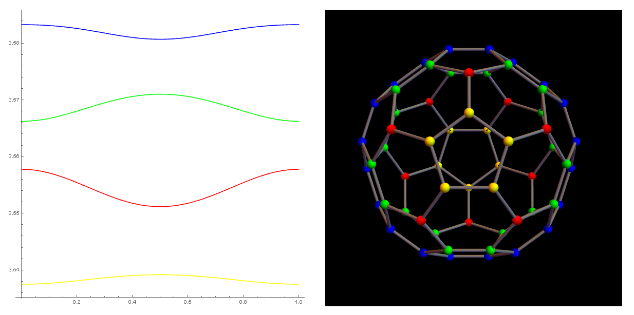
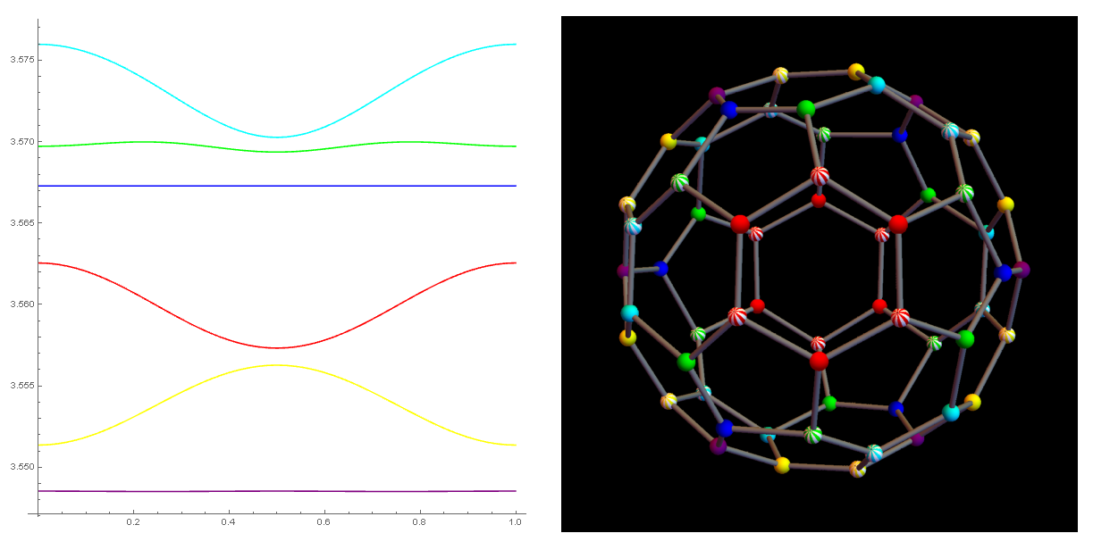
Figure 5: Top: Solutions from eigenvalue $j=2$ with symmetries $({D_{5}^{p}}\prescript{}{}{\times}D_{1})$. Middle: Solution from eigenvalue $j=3$ with symmetries ${({D_{3}^{p}}\prescript{{\mathbb{Z}_{3}^{p}}}{}{\times}_{\mathbb{Z}_{2}}D_{2})}$. Bottom: Solution from eigenvalue $j=3$ with symmetries $({A_{4}^{p}}\prescript{{A_{4}}}{}{\times}_{\mathbb{Z}_{2}}D_{2})$

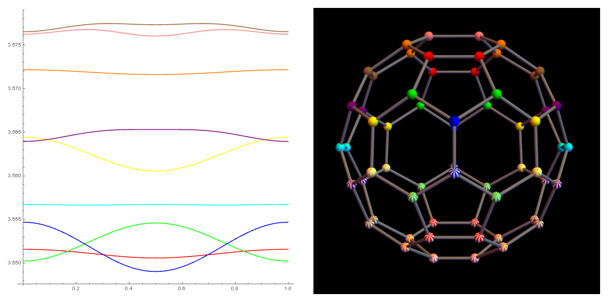
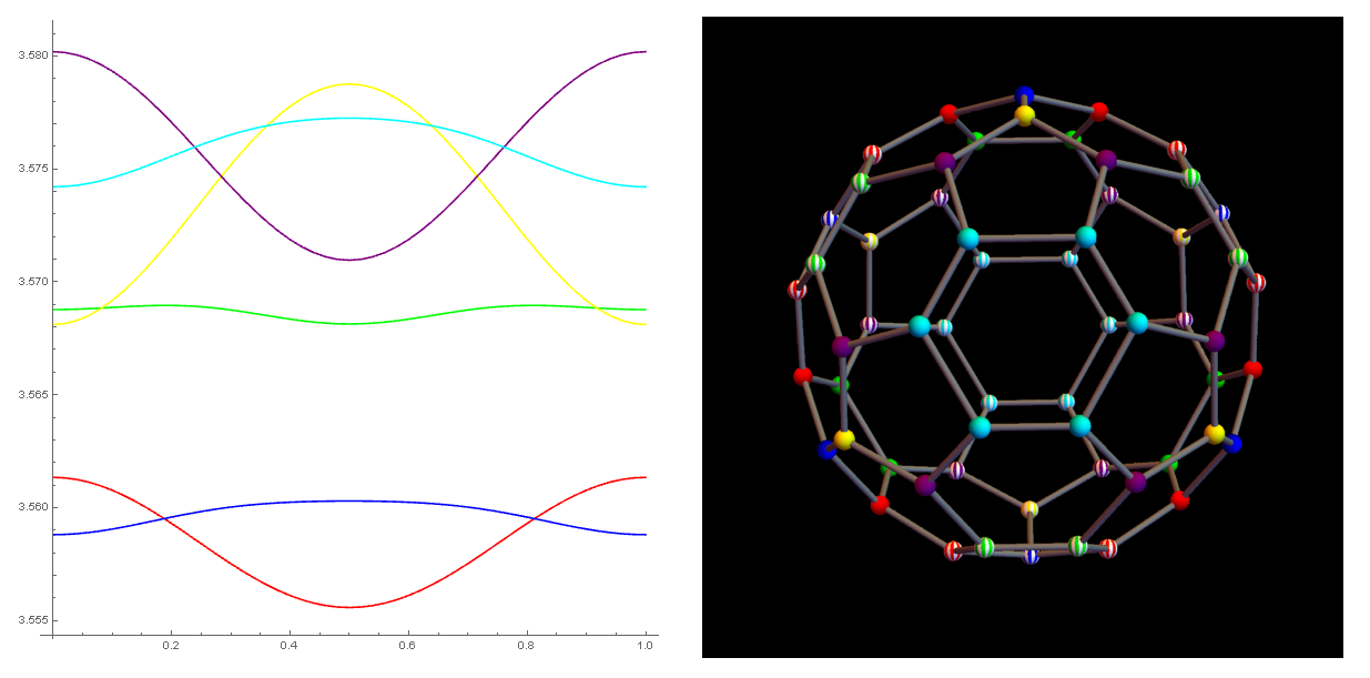
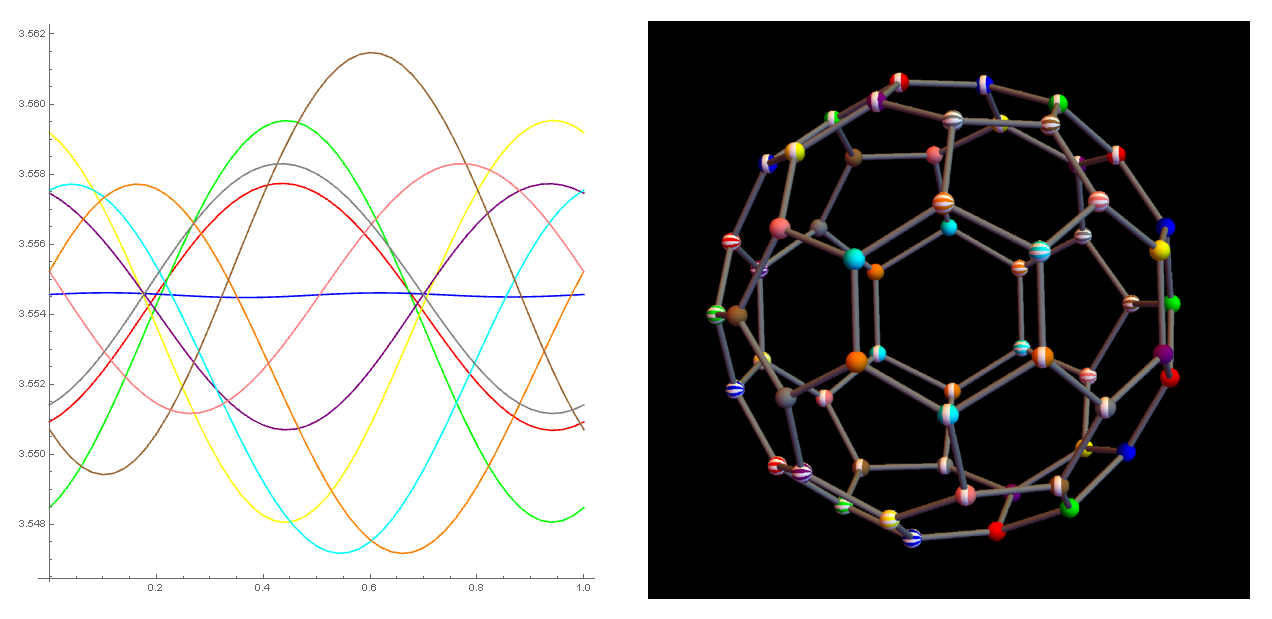
Figure 6: Top: Solutions from eigenvalue $j=4$ with symmetries $({V_{4}^{p}}\prescript{{V_{4}^{z}}}{}{\times}_{\mathbb{Z}_{2}}D_{2})$. Middle: Solutions from eigenvalue $j=5$ with symmetries $({D_{3}^{p}}\prescript{{\mathbb{Z}_{1}}}{}{\times}_{D_{6}}D_{6})$. Bottom: Solutions from eigenvalue $j=9$ with symmetries ${({D_{3}^{p}}\prescript{{\mathbb{Z}_{1}^{p}}}{}{\times}_{D_{3}}D_{3})}$.

The map $\varphi_{1}(x)$ is computed numerically using a Runge-Kutta integrator.  A first solution of $F=0$ is obtained by applying a Newton method in the approximating solution obtained by solving the linearized Hamiltonian system. The family of periodic solutions is computed numerically using a pseudo-arclength procedure to continue the solutions of $F=0$.

We present the results of our numerical computations in Figures 5 and 6. The position of the atoms in space are in the right columns. The atoms with the same color have oscillations related by a rotation or inversion in $O(3)$. In addition, atoms with the same color but different texture describe oscillations that are related by the inversion coupled with a phase shift in time. In the left columns of Figures 5 and 6 we illustrate the norm of the atoms oscillating in time.

Appendix

Appendix A Equivariant Gradient Degree

For an Euclidean space $V$ we denote by $B(V)$ the open unit ball in $V$, and for $x$, $y\in V:=\mathbb{R}^{n}$ we will denote by $x\bullet y$ the standard inner product in $V$.

We assume that $G$ stands for a compact Lie group and that all considered subgroups of $G$ are closed. For a subgroup $H\leq G$, $N\left(H\right)$ stands for the normalizer of $H$ in $G$, and $W\left(H\right)=N\left(H\right)/H$ denotes the Weyl group of $H$ in $G$. We denote by $\left(H\right)$ the conjugacy class of $H$ in $G$ and use the notations $\Phi\left(G\right):=\left\{\left(H\right):H\;\;\text{is a subgroup of }\;G\right\}$ and $\Phi_{n}\left(G\right):=\left\{\left(H\right)\in\Phi\left(G\right):\text{{dim\thinspace}}W\left(H\right)=n\right\}$. The set $\Phi\left(G\right)$ has a natural partial order given by: $\left(H\right)\leq\left(K\right)\;\;\Longleftrightarrow\;\;\exists_{g\in G}\;\;gHg^{-1}\leq K$.

For a $G$-space $X$ and $x\in X$, we put $G_{x}:=\left\{g\in G:\;gx=x\right\}$ to denote the isotropy group of $x$, $G\left(x\right):=\left\{gx:\;g\in G\right\}$ to denote the orbit of $x$, and the conjugacy class $\left(G_{x}\right):=\left\{H\subset G:\;\exists_{g\in G}\;\;G_{x}=g^{-1}Hg\right\}$ will be called the orbit type of $x$, and $\Phi(G;X):=\{(G_{x}):x\in X\}$ will stand for the set of all the orbit types in $X$. We also put $\Phi_{n}(G;X):=\Phi(G;X)\cap\Phi_{n}(G)$.

For a subgroup $H\leq G$, we write $X^{H}:=\left\{x\in X:\;G_{x}\geq H\right\}$ to denote the $H$-fixed point space of $H$. The orbit space for a $G$-space $X$ will be denoted by $X/G$.

As any compact Lie group admits only countably many non-equivalent real irreducible representations, given a compact Lie group $G$, we will assume that we have a complete list of all real irreducible representations, denoted $\mathcal{V}_{i}$, $i=0$, $1$, $\ldots$, which could also be identified by the character list $\{\chi_{i}\}$. We refer to [3] for examples of such lists and the related notation.

Any finite-dimensional real $G$-representation $V$ can be decomposed into the direct sum of $G$-invariant subspaces

$$V=V_{0}\oplus V_{1}\oplus\dots\oplus V_{r}\text{,}$$ (24)

called the $G$-isotypical decomposition of $V$, where each isotypical component $V_{i}$ is modeled on the irreducible $G$-representation $\mathcal{V}_{i}$, $i=0,$ $1,$ $\dots,$ $r$, i.e., $V_{i}$ contains all the irreducible subrepresentations of $V$ which are equivalent to $\mathcal{V}_{i}$. Let $V$ be a $G$-representation, $\Omega\subset V$ an open $G$-invariant bounded set and $f:V\to V$ a continuous $G$-equivariant map such that for all $x\in\partial\Omega$ we have $f(x)\not=0$. Then we say that $f$ is an $\Omega$-admissible $G$-map and we call $(f,\Omega)$ an admissible $G$-pair. The set of all admissible $G$-pairs in $V$ will be denoted by $\mathcal{M}^{G}(V)$. We also put $\mathcal{M}^{G}:=\bigcup_{V}\mathcal{M}^{G}(V)$ (here $V$ denotes all possible $G$-representations) to denote the set of all admissible $G$-pair. A map $f:V\to V$ is called a gradient map if there exists a continuously differentiable $\varphi:V\to\mathbb{R}$ such that $f=\nabla\varphi$. We denote by $\mathcal{M}_{\nabla}^{G}(V)$ the subset of $\mathcal{M}^{G}(V)$ consisting of all gradient maps and we define $\mathcal{M}_{\nabla}^{G}:=\bigcup_{V}\mathcal{M}_{\nabla}^{G}(V)$. In the set $\mathcal{M}^{G}(V)$ (resp. $\mathcal{M}_{\nabla}^{G}(V)$) we have the so-called admissible homotopy (resp. admissible gradient homotopy) relation between $(f_{0},\Omega)$ and $(f_{1},\Omega)$, i.e., if $f_{1}$ and $f_{2}$ are homotopic by an homotopy $h:[0,1]\times V\to V$, such that $h_{t}$ belongs to $\mathcal{M}^{G}(V)$ (resp. $\mathcal{M}_{\nabla}^{G}(V)$) for every $t\in[0,1]$.

A.1 Euler and Burnside Rings

The concept of the Euler ring was introduced by T. tom Dieck in [32]. Due to its topological nature, computations of the Euler ring $U(G)$, for a general compact group $G$, may be quite complicated. However, in our case of interest, when $G:=\Gamma\times O(2)$ with $\Gamma$ being a finite group, the Euler ring structure in $U(G)$ can be effectively described by using elementary techniques based on the reduction techniques and the properties of the Euler ring homomorphisms (see [9] for more details).

Let us recall the definition of the Euler ring $U(G)$. As a $\mathbb{Z}$-module, $U(G)$ is the free $\mathbb{Z}$-module generated by $\Phi(G)$, i.e. $U\left(G\right):={\mathbb{Z}}\left[\Phi\left(G\right)\right]$. The ring multiplication is defined on $U(G)$ on generators $\left(H\right)$, $\left(K\right)\in\Phi\left(G\right)$ by

$$\left(H\right)\ast\left(K\right)=\sum_{\left(L\right)\in\Phi\left(G\right)}n_{L}\left(L\right),$$ (25)

where

$$n_{L}:=\chi_{c}\left(\left(G/H\times G/K\right)_{L}/N\left(L\right)\right)$$ (26)

with $\chi_{c}$ the Euler characteristic taken in Alexander-Spanier cohomology with compact support (cf. [31]). We refer to [7] for more details.

The ${\mathbb{Z}}$-module $A\left(G\right):={\mathbb{Z}}\left[\Phi_{0}\left(G\right)\right]$ equipped with the same multiplication as in $U\left(G\right)$ but restricted to generators from $\Phi_{0}\left(G\right)$ is called Burnside ring, i.e.,

$$\left(H\right)\cdot\left(K\right)=\sum_{\left(L\right)}n_{L}\left(L\right),\qquad\left(H\right),\,\left(K\right),\,\left(L\right)\in\Phi_{0}\left(G\right),$$

where $n_{L}$ stands for the number of $(L)$ orbits in $G/H\times G/K$, i.e. $n_{L}:=\left(\left(G/H\times G/K\right)_{L}/N\left(L\right)\right)=\left|\left(G/H\times G/K\right)_{L}/N\left(L\right)\right|$ (here $|X|$ stands for the number of elements in the set $X$). We have the following recurrence formula

$$n_{L}=\frac{n\left(L,K\right)\left|W\left(K\right)\right|n\left(L,\text{ }H\right)\left|W\left(H\right)\right|-{\displaystyle\sum_{\left(\widetilde{L}\right)>\left(L\right)}}n\left(L,\widetilde{L}\right)n_{\widetilde{L}}\left|W\left(\widetilde{L}\right)\right|}{\left|W\left(L\right)\right|},$$ (27)

where

$$n(L,K)=\left|\frac{N(L,K)}{N(K)}\right|,\quad N(L,K):=\{g\in G:gLg^{-1}\subset K\},$$

and $\left(H\right)$, $\left(K\right)$, $(L)$, $(\widetilde{L})$ are taken from $\Phi_{0}\left(G\right)$.

Clearly, the structure of the Burnside ring $A(G)$ is significantly simpler and can be effectively computed. It is also possible to implement the G.A.P. routines in computer programs evaluating Burnside rings products. Notice that $A\left(G\right)$ is a ${\mathbb{Z}}$-submodule of $U\left(G\right)$, but not a subring. However (see [1]), the projection $\pi_{0}:U\left(G\right)\rightarrow A\left(G\right)$ defined on generators $\left(H\right)\in\Phi\left(G\right)$ by

$$\pi_{0}\left(\left(H\right)\right)=\begin{cases}\left(H\right)&\text{ if }\;\left(H\right)\in\Phi_{0}\left(G\right),\\ 0&\text{ otherwise,}\end{cases}$$ (28)

is a ring homomorphism, i.e.,

$$\pi_{0}\left(\left(H\right)\ast\left(K\right)\right)=\pi_{0}\left(\left(H\right)\right)\cdot\pi_{0}\left(\left(K\right)\right),\qquad\left(H\right),\,\left(K\right)\in\Phi\left(G\right),$$

where ‘$\cdot$’ denotes the multiplication in the Burnside ring $A(G)$. The homomorphism $\pi_{0}$ allows to identify the Burnside ring $A\left(G\right)$ as a part of the Euler ring $U\left(G\right)$ and with the help of additional algorithms, the Euler ring structure for $G=\Gamma\times O(2)$ can be completely computed by elementary means (cf. [9]).

A.2 Equivariant Gradient Degree

The existence and properties of the so-called $G$-equivariant gradient degree are presented in the following result from [12]:

Theorem A.1.

There exists a unique map $\nabla_{G}\text{\rm-deg\,}:\mathcal{M}_{\nabla}^{G}\rightarrow U(G)$, which assigns to every $(\nabla\varphi,\Omega)\in\mathcal{M}_{\nabla}^{G}$ an element $\nabla_{G}\text{\rm-deg\,}(\nabla\varphi,\Omega)\in U(G)$, called the $G$-gradient degree of $\nabla\varphi$ on $\Omega$,

$$\nabla_{G}\text{\rm-deg\,}(\nabla\varphi,\Omega)=\sum_{(H)\in\Phi(G)}n_{H}(H_{i})=n_{H_{1}}(H_{1})+\dots+n_{H_{m}}(H_{m}),$$ (29)

satisfying the following properties:

(Existence) If $\nabla_{G}\text{\rm-deg\,}(\nabla\varphi,\Omega)\not=0$, i.e. there is in (29) a non-zero coefficient $n_{H_{i}}$, then exists $u_{0}\in\Omega$ such that $\nabla\varphi(u_{0})=0$ and $(G_{u_{0}})\geq(H_{i})$.

(Additivity) Let $\Omega_{1}$ and $\Omega_{2}$ be two disjoint open $G$-invariant subsets of $\Omega$ such that $(\nabla\varphi)^{-1}(0)\cap\Omega\subset\Omega_{1}\cup\Omega_{2}.$ Then, $\nabla_{G}\text{\rm-deg\,}(\nabla\varphi,\Omega)=\nabla_{G}\text{\rm-deg\,}(\nabla\varphi,\Omega_{1})+\nabla_{G}\text{\rm-deg\,}(\nabla\varphi,\Omega_{2}).$

(Homotopy) If $\nabla_{x}\psi:[0,1]\times V\rightarrow V$ is a $G$-gradient $\Omega$-admissible homotopy, then

$$\nabla_{G}\text{\rm-deg\,}(\nabla_{x}\psi,\Omega)=\text{{constant}}.$$

(Normalization) Let $\varphi\in C_{G}^{2}(V,\mathbb{R})$ be a special $\Omega$-Morse function (cf. [12]) such that $(\nabla\varphi)^{-1}(0)\cap\Omega=G(u_{0})$ and $G_{u_{0}}=H$. Then,

$$\nabla_{G}\text{\rm-deg\,}(\nabla\varphi,\Omega)=(-1)^{\mathrm{m}^{-}(\nabla^{2}\varphi(u_{0}))}\cdot(H),$$

where “$\mathrm{m}^{-}(\cdot)$” stands for the total dimension of all the eigenspaces corresponding to negative eigenvalues of a (symmetric) matrix.

(Multiplicativity) For all $(\nabla\varphi_{1},\Omega_{1})$, $(\nabla\varphi_{2},\Omega_{2})\in\mathcal{M}_{\nabla}^{G}$,

$$\nabla_{G}\text{\rm-deg\,}(\nabla\varphi_{1}\times\nabla\varphi_{2},\Omega_{1}\times\Omega_{2})=\nabla_{G}\text{\rm-deg\,}(\nabla\varphi_{1},\Omega_{1})\ast\nabla_{G}\text{{-deg\thinspace}}(\nabla\varphi_{2},\Omega_{2})$$

where the multiplication ‘$\ast$’ is taken in the Euler ring $U(G)$.

(Functoriality)(cf. [9]) Suppose $G_{o}\leq G$ is a subgroup of a compact Lie group $G$ such that $\text{\rm dim\,}G_{0}=\text{\rm dim\,}G$. Then any gradient admissible $G$-pair $(\nabla\varphi,\Omega)$ is also an admissible $G_{0}$-pair and we have

$$\Psi\left[\nabla_{G}\text{\rm-deg\,}(\nabla\varphi,\Omega).\right]=\nabla_{G_{0}}\text{\rm-deg\,}(\nabla\varphi,\Omega),$$

where $\Psi:U(G)\to U(G_{0})$ is the Euler ring homomorphism induced by the inclusion $\psi:G_{0}\hookrightarrow G$ (see [1]).

Using a standard finite-dimensional approximation scheme, the $G$-equivariant gradient degree can be extended to admissible $G$-pairs in Hilbert $G$-representation. To be more precise, consider a Hilbert $G$-representation $\mathscr{H}$, a $G$-equivariant completely continuous gradient field $\nabla f:\mathscr{H}\to\mathscr{H}$ and an open bounded $G$-invariant set $\Omega\subset\mathscr{H}$, such that $\nabla f$ is $\Omega$-admissible. Then the pair $(\nabla f,\Omega)$ is called a $G$-admissible pair in $\mathscr{H}$. This degree admits the same properties as those listed in Theorem A.1 (cf. [2, 9]).

One of the most important properties of $G$-equivariant gradient degree $\nabla_{G}\text{-deg}(\nabla f,\Omega)$ is that it provides a full equivariant topological classification of the solution set for $\nabla f(x)=0$ and $x\in\Omega$. More precisely, in addition to the properties listed in Theorem A.1, the equivariant gradient degree has also the so-called Universality Property, which says that two $B(V)$-admissible $G$-equivariant gradient maps $\nabla f_{1}$, $\nabla f_{2}:V\to V$ have the same gradient degrees if and only if they are $B(V)$-admissibly gradient homotopic.

Suppose that

$$\nabla_{G}\text{-deg}(\nabla f,\Omega)=n_{1}(H_{1})+n_{2}(H_{2})+\dots+n_{k}(H_{k})+\dots+n_{m}(H_{m}),$$

and $n_{k}\not=0$. Then, by the existence property, there exists a solution $x_{o}\in\Omega$ of $\nabla f(x)=0$, such that $H:=G_{x_{o}}$. In addition, if $(H_{k})$ is a maximal orbit type in $\Omega$, then for any $\Omega$-admissible continuous deformation $\{\nabla f_{t}\}_{t\in[0,1]}$ (in the class of gradient maps) we obtain a continuum of solutions in $\Omega$ to $\nabla f_{t}(x)=0$ that starts at $x_{0}$ for $t=0$ and ends at $x_{1}$ for $t=1$, and $G_{x_{1}}=H$. This property is called Continuation Property.

A.3 Degree on the Slice

Let $\mathscr{H}$ be a Hilbert $G$-representation. Suppose that the orbit $G(u_{o})$ of $u_{o}\in\mathscr{H}$ is contained in a finite-dimensional $G$-invariant subspace, so the $G$-action on that subspace is smooth and $G(u_{o})$ is a smooth submanifold of $\mathscr{H}$. In such a case we call the orbit $G(u_{o})$ finite-dimensional. Denote by $S_{o}\subset\mathscr{H}$ the slice to the orbit $G(u_{o})$ at $u_{o}$. Denote by $V_{o}:=\tau_{u_{o}}G(u_{o})$ the tangent space to $G(u_{o})$ at $u_{o}$. Then $S_{o}=V_{o}^{\perp}$ and $S_{o}$ is a smooth Hilbert $G_{u_{o}}$-representation.

Then we have (cf. [5])

Theorem A.2.

(Slice Principle) Let $\mathscr{H}$ be a Hilbert $G$-representation, $\Omega$ an open $G$-invariant subset in $\mathscr{H}$, and $\varphi:\Omega\rightarrow\mathbb{R}$ a continuously differentiable $G$-invariant functional such that $\nabla\varphi$ is a completely continuous field. Suppose that $u_{o}\in\Omega$ and $G(u_{o})$ is an finite-dimensional isolated critical orbit of $\varphi$ with $S_{o}$ being the slice to the orbit $G(u_{o})$ at $u_{o}$, and $\mathcal{U}$ an isolated tubular neighborhood of $G(u_{o})$. Put $\varphi_{o}:S_{o}\rightarrow\mathbb{R}$ by $\varphi_{o}(v):=\varphi(u_{o}+v)$, $v\in S_{o}$. Then

$$\nabla_{G}\text{\rm-deg\,}(\nabla\varphi,\mathcal{U})=\Theta(\nabla_{G_{u_{o}}}\text{\rm-deg\,}(\nabla\varphi_{o},\mathcal{U}\cap S_{o})),$$ (30)

where $\Theta:U(G_{u_{o}})\rightarrow U(G)$ is homomorphism defined on generators $\Theta(H)=(H)$, $(H)\in\Phi(G_{u_{o}})$.

A.4 $G$-Equivariant Gradient Degree of Linear Maps

Let us establish a computational formula to evaluate the $G$-equivariant degree $\nabla_{G}\text{-deg\thinspace}(\mathscr{A},B(V))$, where $\mathscr{A}:V\rightarrow V$ is a symmetric $G$-equivariant linear isomorphism and $V$ is an orthogonal $G$-representation, i.e., $\mathscr{A}=\nabla\varphi$ for $\varphi(v)=\frac{1}{2}(\mathscr{A}v\bullet v)$, $v\in V$. Consider the $G$-isotypical decomposition (24) of $V$ and put

$$\mathscr{A}_{i}:=\mathscr{A}|_{V_{i}}:V_{i}\rightarrow V_{i},\quad i=0,1,\dots,r.$$

Then, by the multiplicativity property,

$$\nabla_{G}\mbox{-deg}(\mathscr{A},B(V))=\prod_{i}^{r}\nabla_{G}\mbox{-deg}(\mathscr{A}_{i},B(V_{i}))$$ (31)

Take $\xi\in\sigma_{-}(\mathscr{A})$, where $\sigma_{-}(\mathscr{A})$ stands for the negative spectrum of $\mathscr{A}$, and consider the corresponding eigenspace $E(\xi):=\ker(\mathscr{A}-\xi\mbox{Id})$. Define the numbers $m_{i}(\xi)$ by

$$m_{i}(\xi):=\dim\left(E(\xi)\cap V_{i}\right)/\dim\mathcal{V}_{i},$$ (32)

and the so-called gradient $G$-equivariant basic degrees by

$$\nabla\text{-deg}_{\mathcal{V}_{i}}:=\nabla_{G}\mbox{-deg}(-\mbox{Id\,},B(\mathcal{V}_{i})).,\quad i=0,1,2,\dots$$ (33)

Then

$$\nabla_{G}\text{{-deg}}(\mathscr{A},B(V))=\prod_{\xi\in\sigma_{-}(\mathscr{A})}\prod_{i=0}^{r}\left({\nabla\mbox{\rm-deg}_{\mathcal{V}_{i}}}\right)^{m_{i}(\xi)}.$$ (34)

A.5 $\Gamma\times O(2)$-Equivariant Basic Degrees

In order to be able to effectively use the formula (31), it is important to establish the exact values of the gradient $G$-equivariant basic degrees. A direct usage of topological definition (see [12]) of the gradient $G$-equivariant degree to compute the basic degrees $\nabla\text{-deg}_{\mathcal{V}_{i}}$ (given by (33)), may be very complicated for infinite compact Lie groups $G$. However, in the case of the group $G:=\Gamma\times O(2)$ ($\Gamma$ being a finite group), we have effective reduction techniques (see [9, 28]), using the homomorphism $\pi_{0}$ and the Euler ring homomorphism $\Psi:U(\Gamma\times O(2))\to U(\Gamma\times S^{1})$, which allow to establish the exact values of the gradient $\Gamma\times O(2)$-equivariant basic degrees.

To be more precise, let us recall the $G$-equivariant Brouwer degree$G\text{\rm-deg}(f,\Omega)\in A(G)$, which is defined for admissible $G$-pairs $(f,\Omega)\in\mathcal{M}^{G}(V)$ and has similar existence, additivity, homotopy and multiplicativity properties as the gradient degree. It can be computed by applying the following recurrence formula to the usual Brouwer degrees of maps $f^{H}:V^{H}\to V^{H}$, $(H)\in\Phi_{0}(G;V)$, i.e.,

$$G\text{\rm-deg}(f,\Omega)=\sum_{(H)\in\Phi_{0}(G;V)}n_{H}(H),$$

and

$$n_{H}=\frac{\deg(f^{H},\Omega^{H})-\sum_{(L)>(H)}n_{L}\,n(H,L)\,|W(L)|}{|W(H)|}.$$ (35)

In addition, for any gradient admissible $G$-pair $(\nabla\varphi,\Omega)$, the $G$-equivariant Brouwer degree $G\text{\rm-deg}(\nabla\varphi,\Omega)\in A(G)$ is well-defined and we have the following relation (see [9])

$$\pi_{0}\left(\nabla_{G}\text{-deg}(\nabla\varphi,\Omega)\right)=G\text{\rm-deg}(\nabla\varphi,\Omega).$$ (36)

Moreover, the Brouwer $G$-equivariant basic degrees

$$\deg_{\mathcal{V}_{i}}:=G\text{\rm-deg}(-\text{\rm Id\,},B(\mathcal{V}_{i})),\quad i=0,1,2,3,\dots.$$

satisfy

$$\deg_{\mathcal{V}_{i}}=\pi_{0}\left[\nabla\text{-deg}_{\mathcal{V}_{i}}\right],\quad i=0,1,2,3\dots$$ (37)

Therefore, by (37),

$$\nabla\text{-deg}_{\mathcal{V}_{i}}=\deg_{\mathcal{V}_{i}}+\sum_{(H)\in\Phi_{1}(G;\mathcal{V}_{i})}x_{H}(H),$$

with the integers $x_{H}$ that need to be determined by other means.

Since the gradient basic degrees $\widetilde{\deg}_{\mathcal{V}_{i}}$ for the group $\Gamma\times S^{1}$ are well-known, one can apply the Euler ring homomorphism $\Psi:U(\Gamma\times O(2))\to U(\Gamma\times S^{1})$ to determine these coefficients (see [9]) by using the relation

$$\widetilde{\deg}_{\mathcal{V}_{i}}=\Psi\left[\deg_{\mathcal{V}_{i}}\right]+\sum_{(H)\in\Phi_{1}(G;\mathcal{V}_{i})}x_{H}\Psi(H),$$

(here we assume that $S^{1}$ acts nontrivially on $\mathcal{V}_{i}$). The Euler ring homomorphism $\Psi:U(\Gamma\times O(2))\to U(\Gamma\times S^{1})$ is defined on the generators by

$$\Psi(H) =\begin{cases}2(K)&\text{ if }\;\;K=H\text{ and }K\sim K^{\prime}\text{ in }\Gamma\times SO(2),\\ (K)+(K^{\prime})&\text{ if }\;\;K=H\text{ and }K\not\sim K^{\prime}\text{ in }\Gamma\times SO(2),\\ (K)&\text{ if }\;\;K\not=H,\end{cases}$$ (38)

where $K:=H\cap\Gamma\times SO(2)$, $K^{\prime}:=\kappa H\kappa\cap\Gamma\times SO(2)$.

The formula (35) allows the usage of computational programs based on G.A.P. platform to obtain exact symbolic evaluation of the $G$-equivariant Brouwer degree of linear isomorphisms for a large class of classical groups and their products (see [36]).

A.6 Gradient $I\times O(2)$-Equivariant Basic Degrees

We used GAP programming (all the GAP routines are available for download at the website listed in [36]) to classify all the conjugacy classes of closed subgroups in $G:=I\times O(2)$. We also computed the following basic gradient degrees (corresponding to the irreducible $G$-representations associated to the characters listed in Table 2), where we use red color to indicate the maximal orbit types (in the class of $2\pi$-periodic functions $x:\mathbb{R}\to V$ with Fourier mode $1$).

$$\nabla\mbox{\rm-}\deg_{\mathcal{V}_{1,1}}=\; -{\color[rgb]{1,0,0}({A_{5}^{p}}\prescript{}{}{\times}D_{1})}+({A_{5}^{p}}\prescript{}{}{\times}O(2)),$$

$$\nabla\mbox{\rm-}\deg_{\mathcal{V}_{2,1}}=\; -{\color[rgb]{1,0,0}({D_{3}^{p}}\prescript{{\mathbb{Z}_{3}^{p}}}{}{\times}_{\mathbb{Z}_{2}}D_{2})}-{\color[rgb]{1,0,0}({V_{4}^{p}}\prescript{{\mathbb{Z}_{2}^{p}}}{}{\times}_{\mathbb{Z}_{2}}D_{2})}+2({\mathbb{Z}_{2}^{p}}\prescript{{\mathbb{Z}_{1}^{p}}}{}{\times}_{\mathbb{Z}_{2}}D_{2})-{\color[rgb]{1,0,0}({A_{4}^{p}}\prescript{}{}{\times}D_{1})}$$

$$-{\color[rgb]{1,0,0}({D_{3}^{p}}\prescript{}{}{\times}D_{1})}+2({\mathbb{Z}_{3}^{p}}\prescript{}{}{\times}D_{1})+2({\mathbb{Z}_{2}^{p}}\prescript{}{}{\times}D_{1})-2({\mathbb{Z}_{1}^{p}}\prescript{}{}{\times}D_{1})$$

$$-{\color[rgb]{1,0,0}({D_{5}^{p}}\prescript{{\mathbb{Z}_{1}^{p}}}{}{\times}^{{1}}_{D_{5}}D_{5})}-{\color[rgb]{1,0,0}({D_{5}^{p}}\prescript{{\mathbb{Z}_{1}^{p}}}{}{\times}^{{2}}_{D_{5}}D_{5})}-{\color[rgb]{1,0,0}({D_{3}^{p}}\prescript{{\mathbb{Z}_{1}^{p}}}{}{\times}_{D_{3}}D_{3})}+({V_{4}^{p}}\prescript{{\mathbb{Z}_{1}^{p}}}{}{\times}_{D_{2}}D_{2})$$

$$+({D_{3}^{p}}\prescript{{\mathbb{Z}_{3}^{p}}}{}{\times}_{D_{1}}D_{1})+({V_{4}^{p}}\prescript{{\mathbb{Z}_{2}^{p}}}{}{\times}_{D_{1}}D_{1})+({A_{5}^{p}}\prescript{}{}{\times}O(2))$$

$$-(\mathbb{Z}_{3}^{p}\prescript{}{}{\times}\mathbb{Z}_{1})-(\mathbb{Z}_{2}^{p}\prescript{}{}{\times}\mathbb{Z}_{1})+(\mathbb{Z}_{1}^{p}\prescript{}{}{\times}\mathbb{Z}_{1}),$$

$$\nabla\mbox{\rm-}\deg_{\mathcal{V}_{3,1}}=\; -{\color[rgb]{1,0,0}({V_{4}^{p}}\prescript{{\mathbb{Z}_{2}^{p}}}{}{\times}_{\mathbb{Z}_{2}}D_{2})}+({\mathbb{Z}_{2}^{p}}\prescript{{\mathbb{Z}_{1}^{p}}}{}{\times}_{\mathbb{Z}_{2}}D_{2})-{\color[rgb]{1,0,0}({D_{5}^{p}}\prescript{}{}{\times}D_{1})}-{\color[rgb]{1,0,0}({D_{3}^{p}}\prescript{}{}{\times}D_{1})}$$

$$+2({\mathbb{Z}_{2}^{p}}\prescript{}{}{\times}D_{1})-({\mathbb{Z}_{1}^{p}}\prescript{}{}{\times}D_{1})-{\color[rgb]{1,0,0}({D_{5}^{p}}\prescript{{\mathbb{Z}_{1}^{p}}}{}{\times}^{{1}}_{D_{5}}D_{5})}-{\color[rgb]{1,0,0}({D_{5}^{p}}\prescript{{\mathbb{Z}_{1}^{p}}}{}{\times}^{{2}}_{D_{5}}D_{5})}$$

$$+({V_{4}^{p}}\prescript{{\mathbb{Z}_{1}^{p}}}{}{\times}_{D_{2}}D_{2})+({\mathbb{Z}_{2}^{p}}\prescript{{\mathbb{Z}_{1}^{p}}}{}{\times}_{D_{1}}D_{1})+({A_{5}^{p}}\prescript{}{}{\times}O(2))$$

$$-{\color[rgb]{1,0,0}(A_{4}^{p}\prescript{V_{4}^{p}}{}{\times}_{\mathbb{Z}_{3}}\mathbb{Z}_{3})}-(\mathbb{Z}_{2}^{p}\prescript{\mathbb{Z}_{1}^{p}}{}{\times}_{\mathbb{Z}_{2}}\mathbb{Z}_{2}),$$

$$\nabla\mbox{\rm-}\deg_{\mathcal{V}_{4,1}}=\; -{\color[rgb]{1,0,0}({D_{5}^{p}}\prescript{{\mathbb{Z}_{5}^{p}}}{}{\times}_{\mathbb{Z}_{2}}D_{2})}-{\color[rgb]{1,0,0}({D_{3}^{p}}\prescript{{\mathbb{Z}_{3}^{p}}}{}{\times}_{\mathbb{Z}_{2}}D_{2})}-{\color[rgb]{1,0,0}({V_{4}^{p}}\prescript{{\mathbb{Z}_{2}^{p}}}{}{\times}_{\mathbb{Z}_{2}}D_{2})}+3({\mathbb{Z}_{2}^{p}}\prescript{{\mathbb{Z}_{1}^{p}}}{}{\times}_{\mathbb{Z}_{2}}D_{2})$$

$$-({\mathbb{Z}_{1}^{p}}\prescript{}{}{\times}D_{1})-{\color[rgb]{1,0,0}({D_{5}^{p}}\prescript{{\mathbb{Z}_{1}^{p}}}{}{\times}^{{1}}_{D_{5}}D_{5})}-{\color[rgb]{1,0,0}({D_{3}^{p}}\prescript{{\mathbb{Z}_{1}^{p}}}{}{\times}_{D_{3}}D_{3})}+({V_{4}^{p}}\prescript{{\mathbb{Z}_{1}^{p}}}{}{\times}_{D_{2}}D_{2})$$

$$+({\mathbb{Z}_{2}^{p}}\prescript{{\mathbb{Z}_{1}^{p}}}{}{\times}_{D_{1}}D_{1})+({A_{5}^{p}}\prescript{}{}{\times}O(2))-(\mathbb{Z}_{2}^{p}\prescript{\mathbb{Z}_{1}^{p}}{}{\times}_{\mathbb{Z}_{2}}\mathbb{Z}_{2}),$$

$$\nabla\mbox{\rm-}\deg_{\mathcal{V}_{5,1}}=\; -{\color[rgb]{1,0,0}({D_{5}^{p}}\prescript{{\mathbb{Z}_{5}^{p}}}{}{\times}_{\mathbb{Z}_{2}}D_{2})}-{\color[rgb]{1,0,0}({D_{3}^{p}}\prescript{{\mathbb{Z}_{3}^{p}}}{}{\times}_{\mathbb{Z}_{2}}D_{2})}-{\color[rgb]{1,0,0}({V_{4}^{p}}\prescript{{\mathbb{Z}_{2}^{p}}}{}{\times}_{\mathbb{Z}_{2}}D_{2})}+3({\mathbb{Z}_{2}^{p}}\prescript{{\mathbb{Z}_{1}^{p}}}{}{\times}_{\mathbb{Z}_{2}}D_{2})$$

$$-({\mathbb{Z}_{1}^{p}}\prescript{}{}{\times}D_{1})-{\color[rgb]{1,0,0}({D_{5}^{p}}\prescript{{\mathbb{Z}_{1}^{p}}}{}{\times}^{{2}}_{D_{5}}D_{5})}-{\color[rgb]{1,0,0}({D_{3}^{p}}\prescript{{\mathbb{Z}_{1}^{p}}}{}{\times}_{D_{3}}D_{3})}+({V_{4}^{p}}\prescript{{\mathbb{Z}_{1}^{p}}}{}{\times}_{D_{2}}D_{2})$$

$$+({\mathbb{Z}_{2}^{p}}\prescript{{\mathbb{Z}_{1}^{p}}}{}{\times}_{D_{1}}D_{1})+({A_{5}^{p}}\prescript{}{}{\times}O(2))-(\mathbb{Z}_{2}^{p}\prescript{\mathbb{Z}_{1}^{p}}{}{\times}_{\mathbb{Z}_{2}}\mathbb{Z}_{2})$$

$$\nabla\mbox{\rm-}\deg_{\mathcal{V}_{-1,1}}=\; -{\color[rgb]{1,0,0}({A_{5}^{p}}\prescript{{A_{5}}}{}{\times}_{\mathbb{Z}_{2}}D_{2})}+({A_{5}^{p}}\prescript{}{}{\times}O(2)),$$

$$\nabla\mbox{\rm-}\deg_{\mathcal{V}_{-2,1}}=\; -{\color[rgb]{1,0,0}({A_{4}^{p}}\prescript{{A_{4}}}{}{\times}_{\mathbb{Z}_{2}}D_{2})}-{\color[rgb]{1,0,0}({D_{3}^{p}}\prescript{{D_{3}^{z}}}{}{\times}_{\mathbb{Z}_{2}}D_{2})}-{\color[rgb]{1,0,0}({D_{3}^{p}}\prescript{{D_{3}}}{}{\times}_{\mathbb{Z}_{2}}D_{2})}-{\color[rgb]{1,0,0}({V_{4}^{p}}\prescript{{V_{4}^{z}}}{}{\times}_{\mathbb{Z}_{2}}D_{2})}$$

$$+2({\mathbb{Z}_{3}^{p}}\prescript{{\mathbb{Z}_{3}}}{}{\times}_{\mathbb{Z}_{2}}D_{2})+2({\mathbb{Z}_{2}^{p}}\prescript{{\mathbb{Z}_{2}^{z}}}{}{\times}_{\mathbb{Z}_{2}}D_{2})+2({\mathbb{Z}_{2}^{p}}\prescript{{\mathbb{Z}_{2}}}{}{\times}_{\mathbb{Z}_{2}}D_{2})-2({\mathbb{Z}_{1}^{p}}\prescript{{\mathbb{Z}_{1}}}{}{\times}_{\mathbb{Z}_{2}}D_{2})$$

$$-{\color[rgb]{1,0,0}({D_{5}^{p}}\prescript{{\mathbb{Z}_{1}}}{}{\times}^{{1}}_{D_{10}}D_{10})}-{\color[rgb]{1,0,0}({D_{5}^{p}}\prescript{{\mathbb{Z}_{1}}}{}{\times}^{{2}}_{D_{10}}D_{10})}-{\color[rgb]{1,0,0}({D_{3}^{p}}\prescript{{\mathbb{Z}_{1}}}{}{\times}_{D_{6}}D_{6})}+({D_{3}^{p}}\prescript{{\mathbb{Z}_{3}}}{}{\times}^{{\mathbb{Z}_{3}^{p}}}_{D_{2}}D_{2})$$

$$+({V_{4}^{p}}\prescript{{\mathbb{Z}_{2}^{z}}}{}{\times}^{{\mathbb{Z}_{2}^{p}}}_{D_{2}}D_{2})+({V_{4}^{p}}\prescript{{\mathbb{Z}_{2}}}{}{\times}^{{\mathbb{Z}_{2}^{p}}}_{D_{2}}D_{2})+({A_{5}^{p}}\prescript{}{}{\times}O(2))+(\mathbb{Z}_{1}^{p}\prescript{\mathbb{Z}_{1}}{}{\times}_{\mathbb{Z}_{2}}\mathbb{Z}_{2}),$$

$$\nabla\mbox{\rm-}\deg_{\mathcal{V}_{-3,1}}=\; -{\color[rgb]{1,0,0}({D_{5}^{p}}\prescript{{D_{5}}}{}{\times}_{\mathbb{Z}_{2}}D_{2})}-{\color[rgb]{1,0,0}({D_{3}^{p}}\prescript{{D_{3}}}{}{\times}_{\mathbb{Z}_{2}}D_{2})}-{\color[rgb]{1,0,0}({V_{4}^{p}}\prescript{{V_{4}^{z}}}{}{\times}_{\mathbb{Z}_{2}}D_{2})}+({\mathbb{Z}_{2}^{p}}\prescript{{\mathbb{Z}_{2}^{z}}}{}{\times}_{\mathbb{Z}_{2}}D_{2})$$

$$+2({\mathbb{Z}_{2}^{p}}\prescript{{\mathbb{Z}_{2}}}{}{\times}_{\mathbb{Z}_{2}}D_{2})-({\mathbb{Z}_{1}^{p}}\prescript{{\mathbb{Z}_{1}}}{}{\times}_{\mathbb{Z}_{2}}D_{2})-{\color[rgb]{1,0,0}({D_{5}^{p}}\prescript{{\mathbb{Z}_{1}}}{}{\times}^{{1}}_{D_{10}}D_{10})}-{\color[rgb]{1,0,0}({D_{5}^{p}}\prescript{{\mathbb{Z}_{1}}}{}{\times}^{{2}}_{D_{10}}D_{10})}$$

$$+({V_{4}^{p}}\prescript{{\mathbb{Z}_{2}^{z}}}{}{\times}^{{\mathbb{Z}_{2}^{p}}}_{D_{2}}D_{2})+({\mathbb{Z}_{2}^{p}}\prescript{{\mathbb{Z}_{1}}}{}{\times}^{{\mathbb{Z}_{1}^{p}}}_{D_{2}}D_{2})+({A_{5}^{p}}\prescript{}{}{\times}O(2))$$

$$-{\color[rgb]{1,0,0}(A_{4}^{p}\prescript{V_{4}}{}{\times}_{\mathbb{Z}_{6}}\mathbb{Z}_{6})}-(\mathbb{Z}_{2}^{p}\prescript{\mathbb{Z}_{2}^{z}}{}{\times}_{\mathbb{Z}_{2}}\mathbb{Z}_{2}),$$

$$\nabla\mbox{\rm-}\deg_{\mathcal{V}_{-4,1}}=\; -{\color[rgb]{1,0,0}({D_{5}^{p}}\prescript{{D_{5}^{z}}}{}{\times}_{\mathbb{Z}_{2}}D_{2})}-{\color[rgb]{1,0,0}({D_{3}^{p}}\prescript{{D_{3}^{z}}}{}{\times}_{\mathbb{Z}_{2}}D_{2})}-{\color[rgb]{1,0,0}({V_{4}^{p}}\prescript{{V_{4}^{z}}}{}{\times}_{\mathbb{Z}_{2}}D_{2})}+3({\mathbb{Z}_{2}^{p}}\prescript{{\mathbb{Z}_{2}^{z}}}{}{\times}_{\mathbb{Z}_{2}}D_{2})$$

$$-({\mathbb{Z}_{1}^{p}}\prescript{{\mathbb{Z}_{1}}}{}{\times}_{\mathbb{Z}_{2}}D_{2})-{\color[rgb]{1,0,0}({D_{5}^{p}}\prescript{{\mathbb{Z}_{1}}}{}{\times}^{{1}}_{D_{10}}D_{10})}-{\color[rgb]{1,0,0}({D_{3}^{p}}\prescript{{\mathbb{Z}_{1}}}{}{\times}_{D_{6}}D_{6})}+({V_{4}^{p}}\prescript{{\mathbb{Z}_{2}^{z}}}{}{\times}^{{\mathbb{Z}_{2}^{p}}}_{D_{2}}D_{2})$$

$$+({\mathbb{Z}_{2}^{p}}\prescript{{\mathbb{Z}_{1}}}{}{\times}^{{\mathbb{Z}_{1}^{p}}}_{D_{2}}D_{2})+({A_{5}^{p}}\prescript{}{}{\times}O(2))-(\mathbb{Z}_{2}^{p}\prescript{\mathbb{Z}_{2}^{z}}{}{\times}_{\mathbb{Z}_{2}}\mathbb{Z}_{2}),$$

$$\nabla\mbox{\rm-}\deg_{\mathcal{V}_{-5,1}}=\; -{\color[rgb]{1,0,0}({D_{5}^{p}}\prescript{{D_{5}^{z}}}{}{\times}_{\mathbb{Z}_{2}}D_{2})}-{\color[rgb]{1,0,0}({D_{3}^{p}}\prescript{{D_{3}^{z}}}{}{\times}_{\mathbb{Z}_{2}}D_{2})}-{\color[rgb]{1,0,0}({V_{4}^{p}}\prescript{{V_{4}^{z}}}{}{\times}_{\mathbb{Z}_{2}}D_{2})}+3({\mathbb{Z}_{2}^{p}}\prescript{{\mathbb{Z}_{2}^{z}}}{}{\times}_{\mathbb{Z}_{2}}D_{2})$$

$$-({\mathbb{Z}_{1}^{p}}\prescript{{\mathbb{Z}_{1}}}{}{\times}_{\mathbb{Z}_{2}}D_{2})-{\color[rgb]{1,0,0}({D_{5}^{p}}\prescript{{\mathbb{Z}_{1}}}{}{\times}^{{2}}_{D_{10}}D_{10})}-{\color[rgb]{1,0,0}({D_{3}^{p}}\prescript{{\mathbb{Z}_{1}}}{}{\times}_{D_{6}}D_{6})}+({V_{4}^{p}}\prescript{{\mathbb{Z}_{2}^{z}}}{}{\times}^{{\mathbb{Z}_{2}^{p}}}_{D_{2}}D_{2})$$

$$+({\mathbb{Z}_{2}^{p}}\prescript{{\mathbb{Z}_{1}}}{}{\times}^{{\mathbb{Z}_{1}^{p}}}_{D_{2}}D_{2})+({A_{5}^{p}}\prescript{}{}{\times}O(2))-(\mathbb{Z}_{2}^{p}\prescript{\mathbb{Z}_{2}^{z}}{}{\times}_{\mathbb{Z}_{2}}\mathbb{Z}_{2}),$$

Let us point out that the computational algorithms for the basic degrees truncated to $A(I\times O(2))$ where established in [9], and are now being effectively implemented into a computer software for equivariant gradient degree. Most of the maximal orbit types of periodic vibrations have finite Weyl groups, i.e., they are in the basic gradient degrees truncated to $A(I\times O(2))$. Nevertheless, we have detected in the basic gradient degree of the representations $\mathcal{V}_{\pm 3,1}$ a maximal group with Weyl group of dimension one.

Acknowledgement. C. García was partially supported by PAPIIT-UNAM through grant IA105217. W. Krawcewicz acknowledge partial support from National Science Foundation through grant DMS-1413223 and from National Science Foundation of China through grant no. 11871171.

References

- [1] Z. Balanov, W. Krawcewicz, and H. Ruan. Periodic solutions to -symmetric variational problems: -equivariant gradient degree approach. In Nonlinear analysis and optimization II. Optimization, volume 514 of Contemp. Math., pages 45–84. Amer. Math. Soc., Providence, RI, 2010.
- [2] Z. Balanov, W. Krawcewicz, S. a. Rybicki, and H. Steinlein. A short treatise on the equivariant degree theory and its applications. J. Fixed Point Theory Appl., 8(1):1–74, 2010.
- [3] Z. Balanov, W. Krawcewicz, and H. Steinlein. Applied equivariant degree, volume 1 of AIMS Series on Differential Equations & Dynamical Systems. American Institute of Mathematical Sciences (AIMS), Springfield, MO, 2006.
- [4] I. Berezovik, C. García-Azpeitia, and W. Krawcewicz. Symmetries of nonlinear vibrations in tetrahedral molecular configurations. ArXiv e-prints, 2017.
- [5] I. Berezovik, Q. Hu, and W. Krawcewicz. Dihedral molecular configurations interacting by Lennard-Jones and Coulomb forces. ArXiv e-prints, 2017.
- [6] Z. Berkai, M. Daoudi, N. Mendil, and A. Belghachi. Theoretical study of fullerene (C60) force field at room temperature. Energy Procedia, 74:59–64, 2015. The International Conference on Technologies and Materials for Renewable Energy, Environment and Sustainability –TMREES15.
- [7] T. Bröcker and T. tom Dieck. Representations of compact Lie groups, volume 98 of Graduate Texts in Mathematics. Springer-Verlag, New York, 1985.
- [8] C. H. Choi, M. Kertesz, and L. Mihaly. Vibrational assignment of all 46 fundamentals of C60 and C606-: scaled quantum mechanical results performed in redundant internal coordinates and compared to experiments. Journal of Physical Chemistry A, 104:102–112, 2000.
- [9] M. Dabkowski, W. Krawcewicz, Y. Lv, and H.-P. Wu. Multiple periodic solutions for -symmetric Newtonian systems. J. Differential Equations, 263(10):6684–6730, 2017.
- [10] E. Dancer, K. Geba, and S. Rybicki. Classification of homotopy classes of equivariant gradient maps. Fundamenta Mathematicae - FUND MATH, 185:1–18, 01 2005.
- [11] C. García-Azpeitia and M. Tejada-Wriedt. Molecular chains interacting by Lennard-Jones and Coulomb forces. Qual. Theory Dyn. Syst., 16(3):591–608, 2017.
- [12] K. Gȩba. Degree for gradient equivariant maps and equivariant Conley index. In Topological nonlinear analysis, II (Frascati, 1995), volume 27 of Progr. Nonlinear Differential Equations Appl., pages 247–272. Birkhäuser Boston, Boston, MA, 1997.
- [13] A. Golebiewska and S. Rybicki. Global bifurcations of critical orbits of g-invariant strongly indefinite functionals. Nonlinear Analysis.- TMA, 74:1823Ð1834, 2011.
- [14] M. Golubitsky and I. Stewart. The symmetry perspective, volume 200 of Progress in Mathematics. Birkhäuser Verlag, Basel, 2002. From equilibrium to chaos in phase space and physical space.
- [15] E. Goursat. Sur les substitutions orthogonales et les divisions régulières de l’espace. Ann. Sci. École Norm. Sup. (3), 6:9–102, 1889.
- [16] K. Hedberg, L. Hedberg, D. S. Bethune, C. A. Brown, H. C. Dorn, R. D. Johnson, and M. De Vries. Bond lengths in free molecules of buckminsterfullerene, C60, from gas-phase electron diffraction. Science, 254(5030):410–412, 1991.
- [17] R. B. Hoyle. Shapes and cycles arising at the steady bifurcation with icosahedral symmetry. Physica D: Nonlinear Phenomena, 191(3):261 – 281, 2004.
- [18] J. Ize and A. Vignoli. Equivariant degree theory, volume 8 of De Gruyter Series in Nonlinear Analysis and Applications. Walter de Gruyter & Co., Berlin, 2003.
- [19] I. S. J. Montaldi, M. Roberts. Periodic solutions near equilibria of symmetric hamiltonian systems. Philosophical Transactions of the Royal Society of London A: Mathematical, Physical and Engineering Sciences, 325(1584):237–293, 1988.
- [20] D. Jing and Z. Pan. Molecular vibrational modes of C60 and C70 via finite element method. European Journal of Mechanics - A/Solids, 28(5):948 – 954, 2009.
- [21] W. Krawcewicz and J. Wu. Theory of degrees with applications to bifurcations and differential equations. Canadian Mathematical Society Series of Monographs and Advanced Texts. John Wiley & Sons, Inc., New York, 1997. A Wiley-Interscience Publication.
- [22] H. W. Kroto, J. R. Heath, S. C. Obrien, R. F. Curl, and R. E. Smalley. C(60): Buckminsterfullerene. Nature, 318:162, 1985.
- [23] J. A. Montaldi and R. M. Roberts. Relative equilibria of molecules. Journal of Nonlinear Science, 9(1):53–88, Feb 1999.
- [24] J. Moser. Periodic orbits near an equilibrium and a theorem by alan weinstein. Communications on Pure and Applied Mathematics, 29(6):727–747, 1976.
- [25] F. Muioz-Almaraz, E. Freire, J. Galvin, E. Doedel, and A. Vanderbauwhede. Continuation of periodic orbits in conservative and hamiltonian systems. Physica D: Nonlinear Phenomena, 181(1):1 – 38, 2003.
- [26] L. Nirenberg and C. I. of Mathematical Sciences. Topics in nonlinear functional analysis, 1973-1974. Courant Institute Lecture Notes. Courant Institute of Mathematical Sciences, 1974.
- [27] P. H. Rabinowitz. Some global results for nonlinear eigenvalue problems. Journal of Functional Analysis, 7(3):487 – 513, 1971.
- [28] H. Ruan and S. Rybicki. Applications of equivariant degree for gradient maps to symmetric newtonian systems. 68:1479–1516, 03 2008.
- [29] S. a. Rybicki. Applications of degree for -equivariant gradient maps to variational nonlinear problems with -symmetries. Topol. Methods Nonlinear Anal., 9(2):383–417, 1997.
- [30] P. Schwerdtfeger, L. N. Wirz, and J. Avery. The topology of fullerenes. Wiley Interdisciplinary Reviews: Computational Molecular Science, 5(1):96–145, 2015.
- [31] E. H. Spanier. Algebraic topology. McGraw-Hill Book Co., New York-Toronto, Ont.-London, 1966.
- [32] T. tom Dieck. Transformation groups, volume 8 of De Gruyter Studies in Mathematics. Walter de Gruyter & Co., Berlin, 1987.
- [33] J. H. Walther, R. Jaffe, T. Halicioglu, and P. Koumoutsakos. Molecular dynamics simulations of carbon nanotubes in water. In Studying Turbulence Using Numerical Simulation Databases - VIII, pages 5–20. Center for Turbulence Research, 2000. Proceedings of the 2000 Summer Program.
- [34] D. E. Weeks and W. G. Harter. Rotation–vibration spectra of icosahedral molecules. II. icosahedral symmetry, vibrational eigenfrequencies, and normal modes of buckminsterfullerene. The Journal of Chemical Physics, 90(9):4744–4771, 1989.
- [35] A. Weinstein. Normal modes for nonlinear hamiltonian systems. Inventiones mathematicae, 20(1):47–57, Mar 1973.
- [36] H.-P. Wu. A program for the computations of Burnside ring . http://bitbucket.org/psistwu/gammao2, 2016. Developed at University of Texas at Dallas.
- [37] Z. C. Wu, D. A. Jelski, and T. F. George. Vibrational motions of buckminsterfullerene. Chemical Physics Letters, 137:291–294, 1987.