A refinement of Bennett’s inequality with applications to portfolio optimization

Abstract

A refinement of Bennett’s inequality is introduced which is strictly tighter than the classical bound. The new bound establishes the convergence of the average of independent random variables to its expected value. It also carefully exploits information about the potentially heterogeneous mean, variance, and ceiling of each random variable. The bound is strictly sharper in the homogeneous setting and very often significantly sharper in the heterogeneous setting. The improved convergence rates are obtained by leveraging Lambert’s ${\cal W}$ function. We apply the new bound in a portfolio optimization setting to allocate a budget across investments with heterogeneous returns.

1 Introduction

This article studies how the sum of scalar independent random variables can deviate from its expected value. It extends previous bounds from Hoeffding [4] which exploited information about the range of each random variable. It also outperforms previous bounds from Bennett [1] which also incorporates information about the variance of each random variable as well as a single fixed range on all random variables. The proposed bound simultaneously leverages information about the heterogeneous means, variances and ranges of the random variables to obtain better convergence rates in a wider range of useful settings. These rates give tighter guarantees on the probability a given portfolio will underperform. This permits improved portfolio optimization in settings where second-order information is available while parametric information remains unavailable (as we shall show in Section 5).

Recall Hoeffding’s celebrated inequality [4].

Theorem 1.1 (Hoeffding, 1963).

Given $X_{1},\ldots,X_{n}$ scalar independent random variables bounded as $L_{i}\leq X_{i}\leq M_{i}$ for $i=1,\ldots,n$ then

$$\Pr\left(\frac{1}{n}\sum_{i=1}^{n}X_{i}-\frac{1}{n}\sum_{i=1}^{n}\mathrm{E}[X_{i}]\geq t\right)\leq\exp\left(-2\frac{n^{2}t^{2}}{\sum_{i=1}^{n}(M_{i}-L_{i})^{2}}\right).$$

In some scenarios, we may be given the range of a random variable as well as information about its variance. In those settings, Bennett’s inequality may be more appropriate [1]. Classically, this inequality requires that all the random variables have the same ceiling $M$ and the same mean $\mu$ yet can easily be generalized as follows.

Theorem 1.2 (Bennett, 1962).

For a collection $X_{1},\ldots,X_{n}$ of independent random variables satisfying $X_{i}\leq M_{i}$, $\mathrm{E}[X_{i}]=\mu_{i}$ and $\mathrm{E}[(X_{i}-\mu_{i})^{2}]=\sigma_{i}^{2}$ for $i=1,\ldots,n$ and for any $t\geq 0$, the following holds

$$\Pr\left(\frac{1}{n}\sum_{i=1}^{n}X_{i}-\frac{1}{n}\sum_{i=1}^{n}\mathrm{E}[X_{i}]\geq t\right) \leq \exp\left(-n\frac{v}{s^{2}}h\left(\frac{ts}{v}\right)\right)$$

where $h(x)=(1+x)\ln(1+x)-x$, $s=\max_{i}M_{i}-\mu_{i}$ and $v=\frac{1}{n}\sum_{i=1}^{n}\sigma_{i}^{2}$.

The above theorem looks slightly more general than the classic formula in [1] as well as popular variations of the original theorem in the literature. Specifically, we allow the variables to have heterogeneous means $\mu_{i}$ and heterogeneous ceilings $M_{i}$. In Appendix C, we provide a detailed derivation of this flavor of Bennett’s inequality.

Bernstein’s inequality [2] is obtained by replacing the function $h(x)$ with the function $g(x)=\frac{3x^{2}}{2x+6}$. Since $h(x)\geq g(x)$ for all $x\geq 0$, it is known that Bennett’s inequality is strictly sharper than Bernstein’s inequality. Moreover, Bernstein’s inequality is in turn sharper than Prohorov’s inequality [6] and Chebyshev [10] inequalities. Therefore, it is natural to focus herein on Bennett’s inequality.

Other variations of Bennett’s inequality were provided by Hoeffding in his third theorem [4]. However, these variations further required all variables to have $\mathrm{E}[X_{i}]=0$, a constant variance $\sigma^{2}$ and a constant ceiling $M$. These variations are therefore less useful when the random variables are heterogeneous. Hoeffding’s inequalities were subsequently improved and extended, notably by Talagrand [8, 9] which, under mild conditions, gave tighter bounds by identifying some missing factors.

This article will propose a novel variant of Bennett’s inequality. In the homogeneous case, this variant yields a strictly tighter bound since it avoids using an unnecessary loosening. The new inequality also allows each individual random variable to have its own distinct and heterogeneous range, mean and variance. These heterogeneous properties will be exploited more subtly to obtain a bound that remains tight even if many random variables are drawn from very different distributions. The new bound achieves sharper rates by leveraging Lambert’s ${\cal W}$ function (specifically, the so-called principal value of Lambert’s function). As further explicated in Appendix A, this function is as straightforward to compute as any other and enjoys a number of analytic properties [7].

This article is organized as follows. In Section 2, we derive a refinement of Bennett’s inequality. In Section 3, we numerically explore the sharpness of this bound relative to other classical inequalities in the case of homogeneous random variables which have identical means, variances and ranges. In Section 4, we numerically explore the sharpness of the bound in the heterogeneous case. In Section 5 we discuss applications of the bound in portfolio assessment. The article then concludes with a brief discussion.

2 Refining Bennett’s inequality

Given a sequence of independent random scalar variables $X_{i}$, the following theorem bounds the probability that $\frac{1}{n}\sum_{i=1}^{n}X_{i}$ will deviate above its expected value by more than $t$.

We consider first the case where all the random variables have homogeneous mean, ceiling and variance.

Theorem 2.1.

Let $X_{1},\ldots,X_{n}$ be independent real-valued random variables such that $\mathrm{E}[X_{i}]=\mu$, $\mathrm{E}[(X_{i}-\mu)^{2}]=\sigma^{2}$ and $\Pr(X_{i}\in(-\infty,M])=1$. Then, for any $t\in(0,M-\mu)$, the following inequality holds

$$\Pr\left(\frac{1}{n}\sum_{i=1}^{n}X_{i}-\frac{1}{n}\sum_{i=1}^{n}\mathrm{E}[X_{i}]\geq t\right) \leq e^{-\lambda nt}\left(\frac{\sigma^{2}}{s^{2}}\left(e^{\lambda s}-1-\lambda s\right)+1\right)^{n}$$

where $s=M-\mu$ and

$$\lambda = \frac{1}{t}+\frac{s}{\sigma^{2}}-\frac{1}{s}-\frac{1}{s}{\cal W}\left(\exp\left(\frac{s}{t}+\frac{s^{2}}{\sigma^{2}}-1+\ln\left(\frac{s-t}{t}\right)\right)\right).$$

The above is an immediate consequence of our main theorem which generalizes to the setting of heterogeneous random variables.

Theorem 2.2.

Let $X_{1},\ldots,X_{n}$ be independent real-valued random variables such that $\mathrm{E}[X_{i}]=\mu_{i}$, $\mathrm{E}[(X_{i}-\mu_{i})^{2}]=\sigma_{i}^{2}$ and $\Pr(X_{i}\in(-\infty,M_{i}])=1$. Then, for any $t\in(0,s)$, the following inequality holds

$$\Pr\left(\frac{1}{n}\sum_{i=1}^{n}X_{i}-\frac{1}{n}\sum_{i=1}^{n}\mathrm{E}[X_{i}]\geq t\right) \leq e^{-\lambda nt}\prod_{i=1}^{n}\left(\frac{\sigma_{i}^{2}}{s_{i}^{2}}\left(e^{\lambda s_{i}}-1-\lambda s_{i}\right)+1\right)$$

where

$$\lambda = \frac{1}{{\sum_{i=1}^{n}\frac{s_{i}^{2}}{1-e^{-s_{i}^{2}/\sigma_{i}^{2}}}}}\sum_{i=1}^{n}\frac{s_{i}^{2}\lambda_{i}}{1-e^{-s_{i}^{2}/\sigma_{i}^{2}}}$$

$$\lambda_{i} = \frac{s}{ts_{i}}+\frac{s_{i}}{\sigma_{i}^{2}}-\frac{1}{s_{i}}-\frac{1}{s_{i}}{\cal W}\left(\exp\left(\frac{s}{t}+\frac{s_{i}^{2}}{\sigma_{i}^{2}}-1+\ln\left(\frac{s-t}{t}\right)\right)\right)$$

$$s = \frac{1}{n}\sum_{i=1}^{n}s_{i},\>\>s_{i}\>=\>M_{i}-\mu_{i}.$$

Proof.

Consider the probability of interest

$$\Pr = \Pr\left(\frac{1}{n}\sum_{i=1}^{n}X_{i}-\frac{1}{n}\sum_{i=1}^{n}\mathrm{E}[X_{i}]\geq t\right).$$

Consider translated versions of the random variables $Y_{i}=X_{i}-\mu_{i}$. We now have $\mathrm{E}[Y_{i}]=0$, $\mathrm{E}[Y_{i}^{2}]=\sigma_{i}^{2}$ and $\Pr(Y_{i}\in(-\infty,M_{i}-\mu_{i}])=1$. Applying the change of variables $Y_{i}=X_{i}-\mu_{i}$ does not change the probability of interest

$$\Pr = \Pr\left(\frac{1}{n}\sum_{i=1}^{n}Y_{i}\geq t\right)$$

$$= \Pr\left(e^{\lambda\sum_{i=1}^{n}Y_{i}}\geq e^{\lambda nt}\right)$$

where the second line holds for any $\lambda\geq 0$ by monotonic transformation of the probability. We then apply Markov’s inequality as follows:

$$\Pr \leq \inf_{\lambda\geq 0}e^{-\lambda nt}\mathrm{E}\left[e^{\lambda\sum_{i=1}^{n}Y_{i}}\right]$$

$$= \inf_{\lambda\geq 0}e^{-\lambda nt}\prod_{i=1}^{n}\mathrm{E}[e^{\lambda Y_{i}}].$$

Above, the second line follows from the independence of the random variables. Consider bounding a single term in the product, in other words $\mathrm{E}[e^{\lambda Y_{i}}]$. Begin by the conjecture (which will be subsequently proved) that the following upper bound holds for appropriate choices of the three parameters $(\alpha_{i},\beta_{i},\gamma_{i})$ for all $\lambda\geq 0$:

$$\mathrm{E}[e^{\lambda Y_{i}}] \leq \gamma_{i}\exp(\lambda\alpha_{i})+1-\gamma_{i}-\beta_{i}\lambda.$$

Clearly, when $\lambda=0$, both sides of the conjectured bound are unity and equality is achieved. When $\lambda=0$, the derivative of the left hand side is

$$\left.\frac{\partial\mathrm{E}[e^{\lambda Y_{i}}]}{\partial\lambda}\right|_{\lambda=0}=\mathrm{E}[Y_{i}]=0.$$

For the bound to hold locally around $\lambda=0$ both left hand side and right hand side must have equal derivatives when they attain equality at $\lambda=0$. This tangential contact ensures the bound will not cross the original function as $\lambda$ varies. This forces the following choice for the second parameter

$$\left.\frac{\partial\left(\gamma_{i}\exp(\lambda\alpha_{i})+1-\gamma_{i}-\beta_{i}\lambda\right)}{\partial\lambda}\right|_{\lambda=0} = 0$$

$$\beta_{i} = \gamma_{i}\alpha_{i}.$$

Choose $\alpha_{i}=M_{i}-\mu_{i}$. To satisfy the above tangential contact constraint, it is necessary that $\beta_{i}=\gamma_{i}(M_{i}-\mu_{i})$. The conjectured bound is now

$$\mathrm{E}[e^{\lambda Y_{i}}] \leq \gamma_{i}\exp(\lambda(M_{i}-\mu_{i}))+1-\gamma_{i}-\gamma_{i}(M_{i}-\mu_{i})\lambda.$$

Since the above inequality makes tangential contact, taking second derivatives of both sides with respect to $\lambda$ gives a conservative curvature test to ensure that the bound holds. If the right hand side has higher curvature everywhere and makes tangential contact at $\lambda=0$ then it upper-bounds the left hand side. Taking second derivatives of both sides with respect to $\lambda$ produces the curvature constraint

$$\frac{\partial^{2}\mathrm{E}[e^{\lambda Y_{i}}]}{\partial\lambda^{2}} \leq \frac{\partial^{2}\left(\gamma_{i}\exp(\lambda(M_{i}-\mu_{i}))+1-\gamma_{i}-\gamma_{i}(M_{i}-\mu_{i})\lambda\right)}{\partial\lambda^{2}}$$

$$\mathrm{E}[e^{\lambda Y_{i}}Y_{i}^{2}] \leq \gamma_{i}\exp(\lambda(M_{i}-\mu_{i}))(M_{i}-\mu_{i})^{2}.$$

Divide both sides by $\exp(\lambda(M_{i}-\mu_{i}))$ to obtain

$$\mathrm{E}[e^{\lambda(Y_{i}-(M_{i}-\mu_{i}))}Y_{i}^{2}] \leq \gamma_{i}(M_{i}-\mu_{i})^{2}.$$

Note that $\exp(\lambda(Y_{i}-(M_{i}-\mu_{i}))\leq 1$ inside the expectation since $\lambda\geq 0$ and $Y_{i}\leq M_{i}-\mu_{i}$. Replacing $\exp(\lambda(Y_{i}-(M_{i}-\mu_{i}))$ in the expectation with $1$ gives the following stricter condition on $\gamma_{i}$ to guarantee a bound:

$$\mathrm{E}[e^{\lambda(Y_{i}-(M_{i}-\mu_{i}))}Y_{i}^{2}]\>\leq\>\mathrm{E}[Y_{i}^{2}]\>\leq\>\gamma_{i}(M_{i}-\mu_{i})^{2}.$$

Since $\mathrm{E}[Y_{i}^{2}]=\sigma_{i}^{2}$, the following setting for $\gamma_{i}$ guarantees that the curvature of the upper bound is larger than that of the original function:

$$\gamma_{i} = \frac{\sigma_{i}^{2}}{(M_{i}-\mu_{i})^{2}}.$$

Thus, the conjectured bound holds for any choice of $\lambda\geq 0$ and is tight at $\lambda=0$. Next define $s_{i}=M_{i}-\mu_{i}$ and rewrite the above expression as

$$\mathrm{E}[e^{\lambda Y_{i}}] \leq \frac{\sigma_{i}^{2}}{s_{i}^{2}}\left(\exp(\lambda s_{i}))-1-\lambda s_{i}\right)+1.$$

Apply this upper bound to each individual term in the product

$$\Pr \leq \inf_{\lambda\geq 0}e^{-\lambda nt}\prod_{i=1}^{n}\mathrm{E}[e^{\lambda Y_{i}}]$$

$$\leq \inf_{\lambda\geq 0}e^{-\lambda nt}\prod_{i=1}^{n}\left(\frac{\sigma_{i}^{2}}{s_{i}^{2}}\left(e^{\lambda s_{i}}-1-\lambda s_{i}\right)+1\right).$$

This gives the bound in the theorem $\Pr\leq B(\lambda)$ where

$$B(\lambda) = e^{-\lambda nt}\prod_{i=1}^{n}\left(\frac{\sigma_{i}^{2}}{s_{i}^{2}}\left(e^{\lambda s_{i}}-1-\lambda s_{i}\right)+1\right).$$

What remains is to specify the choice of $\lambda$ to impute into the formula. We next consider ways of finding a good choice for $\lambda$. However, we emphasize that any choice for $\lambda\geq 0$ creates a valid upper bound on the probability $\Pr$.

We start by finding a looser upper bound on $B(\lambda)$ which we will then minimize in order to recover $\lambda$ which we denote by $\lambda^{*}$. We start by considering $n$ arbitrary non-negative scalar variables $t_{1},\ldots,t_{n}$ that sum to $nt$, i.e. $\sum_{i=1}^{n}t_{i}=nt$. We choose to set these $t_{i}$ as follows

$$t_{i} = t\frac{s_{i}}{\frac{1}{n}\sum_{i=1}^{n}s_{i}}\>=\>\frac{ts_{i}}{s}.$$

where we have taken $s=\frac{1}{n}\sum_{i=1}^{n}s_{i}$. Rewrite the current bound as follows

$$B(\lambda) = e^{-\lambda\sum_{i=1}^{n}t_{i}}\prod_{i=1}^{n}\left(\frac{\sigma_{i}^{2}}{s_{i}^{2}}\left(e^{\lambda s_{i}}-1-\lambda s_{i}\right)+1\right)$$

$$= \exp\sum_{i=1}^{n}\left(\log\left(\frac{\sigma_{i}^{2}}{s_{i}^{2}}\left(e^{\lambda s_{i}}-1-\lambda s_{i}\right)+1\right)-\lambda t_{i}\right)$$

$$= \exp\sum_{i=1}^{n}b_{i}(\lambda)$$

where we have defined the terms in the summation as follows

$$b_{i}(\lambda) = \log\left(\frac{\sigma_{i}^{2}}{s_{i}^{2}}\left(e^{\lambda s_{i}}-1-\lambda s_{i}\right)+1\right)-\lambda t_{i}.$$

The minimizer of $b_{i}(\lambda)$ is obtained in closed-form via the Lambert ${\cal W}$ function as follows

$$\lambda_{i}^{*} = \arg\min_{\lambda}b_{i}(\lambda)$$

$$= \frac{1}{t_{i}}+\frac{s_{i}}{\sigma_{i}^{2}}-\frac{1}{s_{i}}-\frac{1}{s_{i}}{\cal W}\left(\exp\left(\frac{s_{i}}{t_{i}}+\frac{s_{i}^{2}}{\sigma_{i}^{2}}-1+\ln\left(\frac{s_{i}-t_{i}}{t_{i}}\right)\right)\right)$$

$$= \frac{s}{ts_{i}}+\frac{s_{i}}{\sigma_{i}^{2}}-\frac{1}{s_{i}}-\frac{1}{s_{i}}{\cal W}\left(\exp\left(\frac{s}{t}+\frac{s_{i}^{2}}{\sigma_{i}^{2}}-1+\ln\left(\frac{s-t}{t}\right)\right)\right)$$

where in the last line we have inserted the choice for $t_{i}$. Note, that Theorem B.1 in the Appendix ensures that the minimizers are non-negative, in other words, $\lambda_{i}^{*}\geq 0.$

Next, derive the curvature of $b_{i}(\lambda)$ and upper-bound it as follows

$$\frac{\partial^{2}b_{i}(\lambda)}{\partial\lambda^{2}} = \frac{\sigma_{i}^{2}e^{\lambda s_{i}}}{\frac{\sigma_{i}^{2}}{s_{i}^{2}}(e^{\lambda s_{i}}-\lambda s_{i}-1)+1}-\left(\frac{\frac{\sigma_{i}^{2}}{s_{i}}(e^{\lambda s_{i}}-1)}{\frac{\sigma_{i}^{2}}{s_{i}^{2}}(e^{\lambda s_{i}}-\lambda s_{i}-1)+1}\right)^{2}$$

$$\leq \frac{\sigma_{i}^{2}e^{\lambda s_{i}}}{\frac{\sigma_{i}^{2}}{s_{i}^{2}}(e^{\lambda s_{i}}-\lambda s_{i}-1)+1}.$$

Above, we bounded the curvature simply by dropping the last negative term. Taking derivatives and setting to zero gives the maximum of the right hand side above which yields $\lambda=s_{i}/\sigma_{i}^{2}$. Inserting this value of $\lambda$ into the bound gives a supremum on the curvature

$$\frac{\partial^{2}b_{i}(\lambda)}{\partial\lambda^{2}} \leq \frac{\sigma_{i}^{2}\exp(s_{i}^{2}/\sigma_{i}^{2})}{\frac{\sigma_{i}^{2}}{s_{i}^{2}}(e^{s_{i}^{2}/\sigma_{i}^{2}}-s_{i}^{2}/\sigma_{i}^{2}-1)+1}$$

$$= \frac{s_{i}^{2}}{1-e^{-s_{i}^{2}/\sigma_{i}^{2}}}.$$

We now form a quadratic upper bound for each $b_{i}(\lambda)$ term as follows,

$$b_{i}(\lambda) \leq \frac{s_{i}^{2}}{1-e^{-s_{i}^{2}/\sigma_{i}^{2}}}\frac{(\lambda-\lambda_{i}^{*})^{2}}{2}+b_{i}(\lambda_{i}^{*}).$$

The above holds since both left hand side and right hand side are equal when $\lambda=\lambda_{i}^{*}$. Furthermore, the gradients of both the left hand side and the right hand side are zero when $\lambda=\lambda_{i}^{*}$. Finally, the curvature of the left hand side is always less than the curvature of the right hand side. Therefore, the quadratic on the right hand side must be an upper bound on $b_{i}(\lambda)$. Replacing each $b_{i}(\lambda)$ term with its corresponding quadratic bound gives an overall upper bound on $B(\lambda)$ as follows

$$B(\lambda) = \exp\left(\sum_{i=1}^{n}b_{i}(\lambda)\right)$$

$$\leq \exp\left(\sum_{i=1}^{n}\frac{s_{i}^{2}}{1-e^{-s_{i}^{2}/\sigma_{i}^{2}}}\frac{(\lambda-\lambda_{i}^{*})^{2}}{2}+b_{i}(\lambda_{i}^{*})\right).$$

It is easy to minimize the right hand side analytically over $\lambda$ to obtain

$$\lambda^{*} = \frac{1}{{\sum_{i=1}^{n}\frac{s_{i}^{2}}{1-e^{-s_{i}^{2}/\sigma_{i}^{2}}}}}\sum_{i=1}^{n}\frac{s_{i}^{2}\lambda_{i}^{*}}{1-e^{-s_{i}^{2}/\sigma_{i}^{2}}}$$

which yields the theorem. ∎

An interesting property of Theorem 2.2 is that it carefully incorporates heterogeneous information about the different random variables. Rather than simply averaging variances (as in Bennett’s inequality), we compute more complicated interactions between the variances $\sigma_{i}^{2}$ and the spreads $s_{i}=M_{i}-\mu_{i}$. This subtle combination of information about the heterogeneous random variables will yield significant improvements over Bennett’s inequality. Furthermore, in the homogeneous setting (which emerges if all $\sigma_{i}=\sigma$ and all $s_{i}=s$), it is clear that the new bound in Theorem 2.1 is circumventing loosening steps in Bennett’s inequality. Therefore, our proposed bounds are strictly tighter than Bennett’s.

We can also consider a counterpart of Theorem 2.2 which uses information about the bottom range on $X_{i}$, namely $L_{i}\leq X_{i}$, instead of the ceiling. Note that it is also straightforward to derive counterparts of Bennett’s and Bernstein’s bounds in such a setting as well.

Theorem 2.3.

Let $X_{1},\ldots,X_{n}$ be independent real-valued random variables such that $\mathrm{E}[X_{i}]=\mu_{i}$, $\mathrm{E}[(X_{i}-\mu_{i})^{2}]=\sigma_{i}^{2}$ and $\Pr(X_{i}\in[L_{i},\infty))=1$. Then, for any $t\in(0,s)$, the following inequality holds

$$\Pr\left(\frac{1}{n}\sum_{i=1}^{n}X_{i}-\frac{1}{n}\sum_{i=1}^{n}\mathrm{E}[X_{i}]\leq-t\right) \leq e^{-\lambda nt}\prod_{i=1}^{n}\left(\frac{\sigma_{i}^{2}}{s_{i}^{2}}\left(e^{\lambda s_{i}}-1-\lambda s_{i}\right)+1\right)$$

where

$$\lambda = \frac{1}{{\sum_{i=1}^{n}\frac{s_{i}^{2}}{1-e^{-s_{i}^{2}/\sigma_{i}^{2}}}}}\sum_{i=1}^{n}\frac{s_{i}^{2}\lambda_{i}}{1-e^{-s_{i}^{2}/\sigma_{i}^{2}}}$$

$$\lambda_{i} = \frac{s}{ts_{i}}+\frac{s_{i}}{\sigma_{i}^{2}}-\frac{1}{s_{i}}-\frac{1}{s_{i}}{\cal W}\left(\exp\left(\frac{s}{t}+\frac{s_{i}^{2}}{\sigma_{i}^{2}}-1+\ln\left(\frac{s-t}{t}\right)\right)\right)$$

$$s = \frac{1}{n}\sum_{i=1}^{n}s_{i},\>\>s_{i}\>=\>\mu_{i}-L_{i}.$$

Proof.

The proof is entirely analogous to the one for Theorem 2.2. ∎

3 Experiments with homogeneous random variables

This section numerically compares the new bound with Hoeffding’s, Bennett’s and Bernstein’s bounds which are well-known classical concentration inequalities. This section will only consider the homogeneous setting, $M_{i}=M$, $\mu_{i}=\mu$ and $\sigma_{i}=\sigma$ for all $i=1,\ldots,n$ random variables.

Specifically, we will compare our bound in Theorem 2.1 against Bennett’s inequality in Theorem 1.2 which uses $h(x)=(1+x)\log(1+x)-x$. Similarly, we consider Bernstein’s inequality [3] which is identical to Bennett’s yet uses $g(x)=\frac{3x^{2}}{2x+6}$ in the place of $h(x)$. Finally, we apply Hoeffding’s inequality as in Theorem 1.1 whose rate has no dependence on the variance of the random variables.

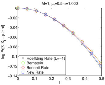
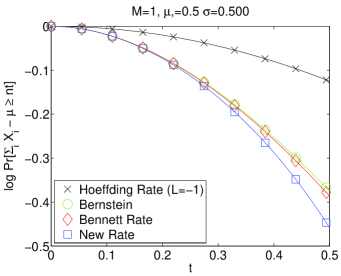
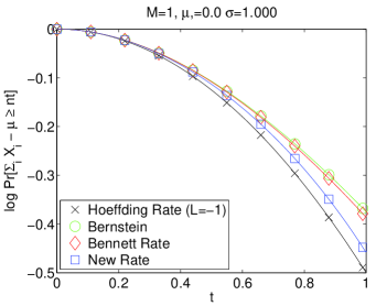
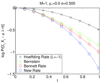
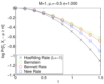
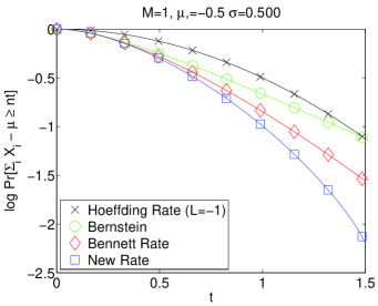
Figure 1: Comparing the four inequalities’ convergence rates for homogeneous random variables under different $\mu$ and $\sigma$ settings. Lower values are better.

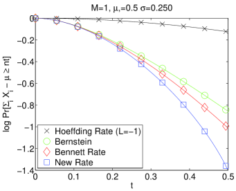
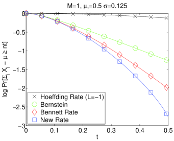
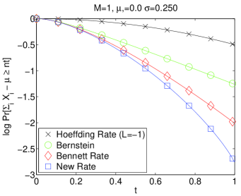
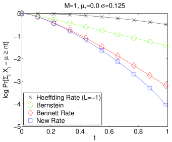
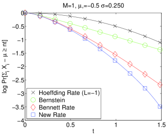
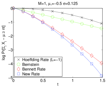
Figure 2: Comparing the four inequalities’ convergence rates for homogeneous random variables under different $\mu$ and $\sigma$ settings. Lower values are better.

To directly compare these bounds, we will explore various values of $M$, $\mu$ and $\sigma$ to see how they compare against each other. For practical visualization purposes, we first note that all bounds scale with $n$ in the same manner. Therefore, without loss of generality, we set $n=1$ throughout our experiments. Furthermore, since we can scale $(M,\mu,\sigma)$ by an arbitrary factor without changing the bounds, we simply lock $M=1$ to remove this source of redundancy in our experimental exploration. Figure 1 and Figure 2, depict the convergence rates for the four different concentration inequalities under various choices of $\mu\in\{-\frac{1}{2},0,\frac{1}{2}\}$ and $\sigma\in\{1,1/2,1/4,1/8\}$. Since Hoeffding’s bound also requires a value for the bottom range of the random variable, $L$, we make a simple arbitrary choice to set it to $L=-M$. In fact, many applications of Bennett and Bernstein typically assume that $|X_{i}|\leq M$ (though it is not strictly necessary to do so). Also, note that setting $L=-M$ does not violate the elementary inequality $\sigma_{i}\leq(M_{i}-L_{i})/2$ in any of our experiments. By observing the log-probability for each bound as $t$ varies, it is possible to see which inequalities are tighter (i.e. yielding an exponentially smaller deviation probability). Bounds with lower (negative) rates indicate faster convergence of the average to its expected value.

Clearly, the new bound is strictly sharper than Bernstein’s and Bennett’s inequalities in the homogeneous setting. In fact, we know that this must be true since Bennett makes an unnecessary loosening step and Bernstein follows it with yet another unnecessary loosening step. Hoeffding’s bound performs poorly unless the variance $\sigma^{2}$ is large, i.e. it is close to the maximum value it can have while still respecting the elementary inequality $\sigma_{i}\leq(M_{i}-L_{i})/2$. At that setting, the variance is essentially providing very little useful information and so the variance-based inequalities (such as Bennett’s, Bernstein’s and the proposed bound) are no longer relevant. Otherwise, the new bound clearly dominates the classical inequalities in our experiments.

It is important to note that these rate quantities will be multiplied by the number of observations $n$ and then exponentiated to obtain bounds on the probability. Therefore, the advantages of the bounds relative to each other will be drastically magnified as $n$ grows.

4 Experiments with heterogeneous random variables

In Section 3 we compared the new bound to classical concentration inequalities when all the random variables are homogeneous. We here consider bounding the probability $\Pr(\frac{1}{n}\sum_{i=1}^{n}X_{i}-\frac{1}{n}\sum_{i=1}\mathrm{E}[X_{i}]\geq t)$ when we deal with independent random variables $X_{i}$ that are not identically distributed but rather have their own distinct heterogeneous values of $M_{i}$, $\mu_{i}$ and $\sigma_{i}$. In these experiments, the advantages of the bound can sometimes be dramatic.

We will consider various random choices of $M_{i}$, $\mu_{i}$, $\sigma_{i}$ and $t$. These synthetic experiments allow us to compare our new inequality relative to the Bernstein, Bennett and Hoeffding inequalities in the heterogeneous setting. To generate synthetic problems, we set $M_{i}$ to be the absolute value of random draws from a white Gaussian (e.g. with zero-mean and unit variance). We set $L_{i}$ to be the negated absolute values drawn from a white Gaussian. We set $\mu_{i}$ equal to a uniform value drawn in the interval $[L_{i},M_{i}]$. We then choose $\sigma_{i}$ uniformly from $[0,\frac{1}{2z}(M_{i}-L_{i})]$ for various choices of $z\geq 1$. This way, we explore different levels of variance without ever violating the elementary inequality $\sigma_{i}\leq(M_{i}-L_{i})/2$. Finally, we set $t$ by sampling a scalar from the uniform distribution and multiplying it by the value $s=\frac{1}{n}\sum_{i=1}^{n}M_{i}-\mu_{i}$ which was introduced in our bound.

We compute the bound using Theorem 2.2 in the heterogeneous setting. To compute Bennett’s inequality in the heterogeneous setting, we use the formula in Theorem 1.2. Similarly, by replacing the $h(x)$ function with the $g(x)$ function, we compute Bernstein’s inequality. All three of these approaches ignore information in the $L_{i}$ values. To compute a bound using Hoeffding’s inequality, we apply Theorem 1.1 which ignores information about the $\sigma_{i}$ and $\mu_{i}$ values.

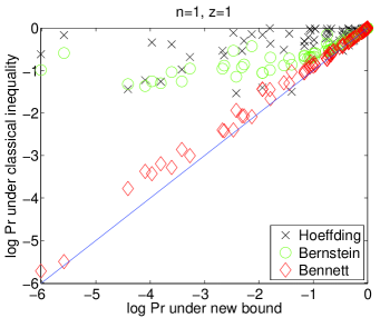
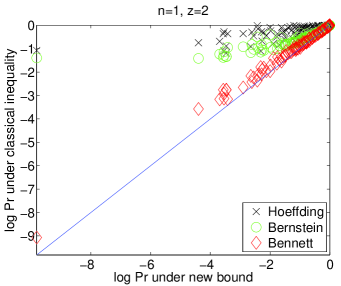
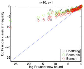
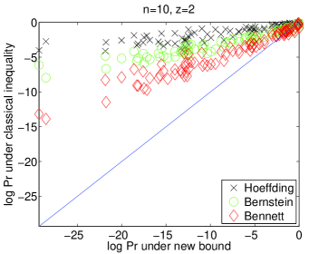
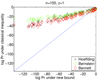
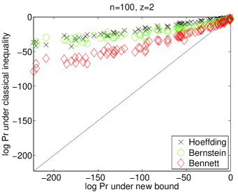
Figure 3: Comparing the classical inequalities with the new bound for heterogeneous random variables where the settings ($L_{i}$, $M_{i}$, $\mu_{i}$ and $\sigma_{i}$) and $t$ are drawn randomly. Specifically $\sigma_{i}$ is drawn from a uniform distribution over $(0,(M_{i}-L_{i})/(2z))$. Various values of $n$ are also explored. A coordinate marker above the blue line indicates that the new bound is performing better than the classical inequality.

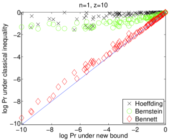
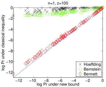
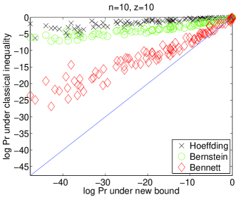
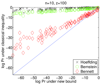
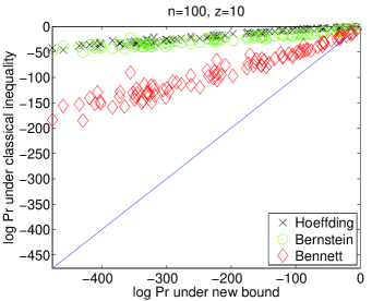
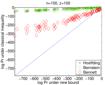
Figure 4: Comparing the classical inequalities with the new bound for heterogeneous random variables where the settings ($L_{i}$, $M_{i}$, $\mu_{i}$ and $\sigma_{i}$) and $t$ are drawn randomly. Specifically $\sigma_{i}$ is drawn from a uniform distribution over $(0,(M_{i}-L_{i})/(2z))$. Various values of $n$ are also explored. A coordinate marker above the blue line indicates that the new bound is performing better than the classical inequality.

In Figure 3 and Figure 4, we see the log-probabilities for the new bound on the x-axis and the log-probabilities for the classical inequalities on the y-axis. Several experiments are shown for $n=1,10,10$ and for $z=1,2,10,100$. Whenever a coordinate marker is above the diagonal line, the new bound is performing better for that particular random experiment. Clearly, the new bound is outperforming Bennett’s, Bernstein’s and Hoeffding’s bounds. When $n=1$ in the top of the figures, we are back to the homogeneous case where the bound must strictly outperform Bennett’s and Bernstein’s inequalities. It also seems to frequently outperform Hoeffding’s. As we increase $n$, the advantages of the bound become even more dramatic in the heterogeneous case. When $z$ is small, the variances $\sigma_{i}^{2}$ are large and potentially close to their maximum allowable values (e.g. prior to violating the elementary inequality $\sigma_{i}\leq(M_{i}-L_{i})/2$). Therefore, variance does not provide much information about the distribution of the random variables. Meanwhile, when $z$ is large, the the variance values are smaller and Hoeffding’s bound becomes extremely loose since it ignores variance information. The new bound seems to frequently outperform the classical inequalities.

5 An application in portfolio optimization

There are many natural applications of Theorems 2.1,  2.2, and  2.3. As a motivating example, consider a financial portfolio with several independent investments. Each investment $i$ will provide a payoff $X_{i}$ from an unknown distribution. We may know a priori the minimum payoff $L_{i}$, the expected payoff $\mu_{i}$ and the variance of the payoff $\sigma_{i}^{2}$ for investment $i$. We are interested in the probability that the sum total of our investments will under-perform its expected value by $t$. For example, we may want to compute the probability that the portfolio will under-perform and produce a total payoff that is smaller than some risk-free payoff $\tau$. The quantity of interest is $\Pr(\sum_{i=1}^{n}X_{i}\leq\tau)$.

Using Theorem 2.3, it is straightforward to upper-bound the probability that a portfolio under-performs. We are given information about each $X_{i}$ such as its $L_{i}$, $\mu_{i}$ and $\sigma_{i}$ and we are given a threshold $\tau$ for the portfolio to be worthwhile. If the total payoff from the investment falls below $\tau$, it has under-performed. Our upper bound holds without making any further parametric assumptions about the distribution of the payoffs $X_{1},\ldots,X_{n}$. Conversely, many practitioners make Gaussian assumptions or parametric assumptions about portfolios and payoff distributions [5]. A non-parametric approach remains agnostic and may be better matched to real-world settings.

Consider the following toy example. We have $n=2$ investments. Investment 1 has an expected payoff of $\mu_{1}=\$30$ with a standard deviation of $\sigma_{1}=\$25$. Investment 2 has an expected payoff of $\mu_{2}=\$100$ with a standard deviation of $\sigma_{2}=\$20$. Investment 1 has a floor on its payoff of $L_{1}=\$25$. Meanwhile, Investment 2 can potentially yield as little as $L_{2}=\$5$ in terms of payout. For the portfolio to be worthwhile, we are told that the total payoff of both investments must be at least $\$74$ (or the average payoff across both investments must be at least $\$37$). Otherwise, the portfolio is under-performing.

According to our new bound in Theorem 2.3, the probability of under-performing is less than 39.1%. We next apply Bennett’s inequality and Bernstein’s inequality to this portfolio problem. Consider Bennett’s inequality in Theorem C.1. Just as we were able to reverse the bound in Theorem 2.2 to obtain Theorem 2.3, it is possible to obtain reversed versions of Bennett’s and Bernstein’s inequalities. Bennett’s says the probability is at most 50.1% and Bernstein says it is at most 57.2%.

To apply Hoeffding’s inequality, we also need an upper bound on the investment’s payouts (e.g. $M_{1}$ and $M_{2}$). Recall the elementary formula $\sigma_{i}\leq(M_{i}-L_{i})/2$. This gives us the most-optimistic value for ${\hat{M}}_{i}=\max(L_{i}+2\sigma_{i},\mu_{i})$. This setting helps tighten the Hoeffding bound as much as possible. Technically, the most-optimistic setting of the Hoeffding bound can be quite erroneous and misleading. In fact, if we make additional assumptions about the problem, then Hoeffding is not actually computing a bound. We are making assumptions that may not be true about the original problem. Nevertheless, we use the heterogeneous $L_{i}$ and imputed ${\hat{M}}_{i}$ in Theorem 1.1. Hoeffding says the probability of under-performing is less than 58.1%. Surprisingly, this is still worse than the (valid) estimate using our novel bound.

The new bound gives the best estimate and shows that the payoff on our investments is more likely to meet the target total payoff of $\$74$ (or an average payoff of $\$37$ across both investments). The bound on the probability of 39.1% shows that the investment portfolio is worth the risk.

Rather than simply bound the probability a given portfolio under-performs, we may wish to find an optimal portfolio. Consider $n$ possible investments where we aim to optimally allocate funds by computing the proportion $\alpha_{i}\geq 0$ of our budget that is allocated to investment $i$ for $i=1,\ldots n$. Clearly, budget proportions sum to unity and therefore $\sum_{i=1}^{n}\alpha_{i}=1$. Let $X_{i}$ represent a random variable which equals the return of the $i$’th investment. Assume we know a priori that $X_{i}$ has mean $\mu_{i}$, deviation $\sigma_{i}$ and floor $L_{i}$. We wish to find $\alpha_{1},\ldots,\alpha_{n}$ that minimize the probability $\Phi$ that the portfolio generates less than some targeted return $\tau$. We can compute $\Phi$ as follows

$$\Phi = \Pr\left(\sum_{i=1}^{n}\alpha_{i}X_{i}\leq\tau\right)\>\>=\>\>\Pr\left(\frac{1}{n}\sum_{i=1}^{n}{\tilde{X}}_{i}-\frac{1}{n}\sum_{i=1}^{n}{\tilde{\mu}}_{i}\leq-\frac{1}{n}t\right).$$

On the right, we have merely rewritten the probability after the change of variables ${\tilde{X}}_{i}=\alpha_{i}X_{i}$ and $t=\sum_{i=1}^{n}{\tilde{\mu}}_{i}-\tau$. The new random variables ${\tilde{X}}_{i}$ have mean ${\tilde{\mu}}_{i}=\alpha_{i}\mu_{i}$, variance ${\tilde{\sigma}_{i}}^{2}=\alpha_{i}^{2}\sigma_{i}^{2}$ and floor ${\tilde{L}}_{i}=\alpha_{i}L_{i}$. Apply Theorem 2.3 which holds for any $\lambda\geq 0$ to obtain

$$\Phi \leq e^{-\lambda t}\prod_{i=1}^{n}\left(\frac{\alpha_{i}^{2}\sigma_{i}^{2}}{\alpha_{i}^{2}(\mu_{i}-L_{i})^{2}}\left(e^{\lambda\alpha_{i}(\mu_{i}-L_{i})}-1-\lambda\alpha_{i}(\mu_{i}-L_{i})\right)+1\right)$$

$$= e^{-\lambda t}\prod_{i=1}^{n}\left(\frac{\sigma_{i}^{2}}{(\mu_{i}-L_{i})^{2}}\left(e^{\lambda_{i}(\mu_{i}-L_{i})}-1-\lambda_{i}(\mu_{i}-L_{i})\right)+1\right)$$

where in the second line we have simply defined $\lambda_{i}=\alpha_{i}\lambda$. Insert the definition of $t$ into the above

$$\Phi \leq e^{-\lambda(\sum_{i=1}^{n}\alpha_{i}(\mu_{i}-\tau))}\prod_{i=1}^{n}\left(\frac{\sigma_{i}^{2}}{(\mu_{i}-L_{i})^{2}}\left(e^{\lambda_{i}(\mu_{i}-L_{i})}-1-\lambda_{i}(\mu_{i}-L_{i})\right)+1\right).$$

Recall that $\lambda_{i}=\lambda\alpha_{i}$ and therefore

$$\Phi \leq \prod_{i=1}^{n}e^{-\lambda_{i}(\mu_{i}-\tau)}\left(\frac{\sigma_{i}^{2}}{(\mu_{i}-L_{i})^{2}}\left(e^{\lambda_{i}(\mu_{i}-L_{i})}-1-\lambda_{i}(\mu_{i}-L_{i})\right)+1\right).$$

We wish to minimize the bound on the right hand side over $\lambda\geq 0$ as well as to minimize it over $\alpha_{i}\geq 0$ for $i=1,\ldots,n$ subject to $\sum_{i=1}^{n}\alpha_{i}=1$. An equivalent problem is to minimize the right hand side of the inequality over $\lambda_{i}\geq 0$ for $i=1,\ldots,n$. The solution can be found by independently minimizing each term in the product $\prod_{i=1}^{n}$ above over the $\lambda_{i}$ that appears in it. The solution for $\lambda_{i}$ is a straightforward reapplication of the derivations in the proof of Theorem 2.2,

$$\lambda_{i} = \frac{1}{\mu_{i}-\tau}+\frac{\mu_{i}-L_{i}}{\sigma_{i}^{2}}-\frac{1}{\mu_{i}-L_{i}}\left(1+{\cal W}\left(\left(\frac{\tau-L_{i}}{\mu_{i}-\tau}\right)e^{\frac{\mu_{i}-L_{i}}{\mu_{i}-\tau}+\frac{(\mu_{i}-L_{i})^{2}}{\sigma_{i}^{2}}-1}\right)\right)$$

and shows that we must require $\tau\in[\mu_{i},L_{i}]$ to obtain valid numerical solutions.

To recover the optimal proportions for our budget, we merely compute $\alpha_{i}=\lambda_{i}/\sum_{i=1}^{n}\lambda_{i}$. Given a $\tau$, to recover the optimized upper bound on $\Phi$, insert the suggested values of $\lambda_{i}$ into the final bound above. Alternatively, rather than specifying a $\tau$ value, a user may prefer to specify how much deviation from the expected return he is willing to tolerate by selecting $t$. In that case, to avoid numerical problems, it is straightforward to see that $t\in(0,\min_{i}(\mu_{i}-L_{i}))$.

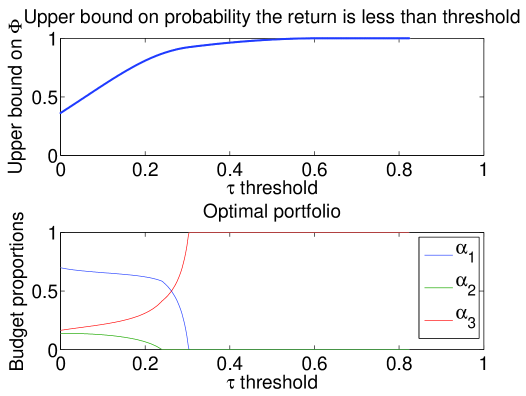
Figure 5: The upper bound on the probability we will obtain a return less than $\tau$ for 3 investments having a floor of 0 and $\mu_{1}=0.3030,\mu_{2}=0.2400,\mu_{3}=0.6178$ with $\sigma_{1}=0.2601,\sigma_{2}=0.5248,\sigma_{3}=0.7645$ (top panel). The corresponding optimal portfolio distribution is plotted for a range of $\tau$ values (bottom panel).

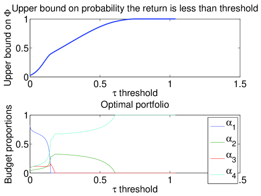
Figure 6: The upper bound on the probability we will obtain a return less than $\tau$ for 4 investments having a floor of 0 and $\mu_{1}=0.1474,\mu_{2}=0.6088,\mu_{3}=0.1785,\mu_{4}=0.7585$ with $\sigma_{1}=0.0593,\sigma_{2}=0.6218,\sigma_{3}=0.2183,\sigma_{4}=0.4597$ (top panel). The corresponding optimal portfolio distribution is plotted for a range of $\tau$ values (bottom panel).

Figure 5 depicts the upper bound on the probability we will obtain a return less than $\tau$ for 3 investments having a floor of 0 and $\mu_{1}=0.3030,\mu_{2}=0.2400,\mu_{3}=0.6178$ with $\sigma_{1}=0.2601,\sigma_{2}=0.5248,\sigma_{3}=0.7645$ (top panel). In the bottom panel, the optimal portfolio distribution is depicted across $\tau$ values. Figure 6 depicts the upper bound on the probability we will obtain a return less than $\tau$ for 4 investments having a floor of 0 and $\mu_{1}=0.1474,\mu_{2}=0.6088,\mu_{3}=0.1785,\mu_{4}=0.7585$ with $\sigma_{1}=0.0593,\sigma_{2}=0.6218,\sigma_{3}=0.2183,\sigma_{4}=0.4597$ (top panel). In the bottom panel, the optimal portfolio distribution is depicted across $\tau$ values.

6 Conclusions

A new bound was proposed that characterizes the convergence of the average of independent bounded random variables towards its expected value. In the homogeneous case, the new bound is strictly sharper than Bennett’s and Bernstein’s inequalities and very often outperforms Hoeffding’s inequality. The bound also readily applies in settings where the random variables are not identically-distributed and may have heterogeneous values for their range, expected value, and variance. In the heterogeneous case, the new bound sometimes dramatically outperforms the classical inequalities as well. The bound appears useful in portfolio optimization as well as potentially other application areas. Deriving the bound involved the use of a peculiar transcendental function known as Lambert’s ${\cal W}$ function. While Lambert’s ${\cal W}$-function has been known since the 1779 paper by Leonhard Euler it has only been popularized in the 1980’s. It may be helpful in the development of other concentration inequalities.

Appendix A Lambert’s W

The Lambert ${\cal W}$ function is defined by the solution of the equation

$${\cal W} = \ln(x)-\ln({\cal W}).$$

Although this function is now integrated in most modern mathematical software, an iterative scheme is provided below to show how it is numerically recovered. The proposed numerical scheme estimates ${\cal W}(x)$ by first guessing a solution ${\cal W}$ and then using the following iterations until convergence:

$${\cal W}\leftarrow{\cal W}-\frac{{\cal W}\exp({\cal W})-x}{({\cal W}+1)\exp({\cal W})-({\cal W}+2)\frac{{\cal W}\exp({\cal W})-x}{2{\cal W}+2}}.$$

An alternative is to manipulate Lambert’s ${\cal W}$ function after the exponentiation operation which yields better numerical results and solves the equation

$${\cal W}(\exp(x)) = x-\ln({\cal W}).$$

If $x\geq 0$, initialize with ${\cal W}=x$ and iterate the following rule to recover ${\cal W}(\exp(x))$:

$${\cal W} \leftarrow {\cal W}-\frac{{\cal W}-\exp(x-{\cal W})}{{\cal W}+1-({\cal W}+2)\frac{{\cal W}-\exp(x-{\cal W})}{2{\cal W}+2}}.$$

If $x\leq 0$, initialize with ${\cal W}=1$ and iterate the following rule to recover ${\cal W}(\exp(x))$:

$${\cal W}\>\leftarrow\>{\cal W}-\frac{{\cal W}\exp({\cal W}-x)-1}{({\cal W}+1)\exp({\cal W}-x)-({\cal W}+2)\frac{{\cal W}\exp({\cal W}-x)-1}{2{\cal W}+2}}.$$

These updates circumvent numerical problems that may arise during evaluation of the bound in Theorems 2.1,  2.2, and  2.3.

Appendix B Closed-form minimizer

The following is useful to prove Theorem 2.2.

Theorem B.1.

The minimizer of $\log(q(e^{\lambda r}-{\lambda r}-1)+1)-\lambda t$ is non-negative for $q\geq 0,r\geq 0$, and $t\in(0,r)$.

Proof.

The minimizer is given by the closed-form expression

$$\lambda^{*} = \frac{1}{t}+\frac{1}{qr}-\frac{1}{r}-\frac{1}{r}{\cal W}\left(\exp\left(\frac{r}{t}+\frac{1}{q}-1+\ln\left(\frac{r-t}{t}\right)\right)\right).$$

Non-negativity therefore implies

$$\frac{r}{t}+\frac{1}{q}-1 \geq {\cal W}\left(\exp\left(\frac{r}{t}+\frac{1}{q}-1+\ln\left(\frac{r-t}{t}\right)\right)\right).$$

Consider the change of variables $x=\frac{r}{t}+\frac{1}{q}-1$ and $y=\frac{1}{q}$. Inserting these into the above required inequality yields

$$x \geq {\cal W}((x-y)e^{x}).$$ (1)

Since, by definition $t\in(0,r)$, it is clear that $x\geq y\geq 0$. Equation 1 is certainly true if the maximization over allowable $y$ on the right hand side (a stricter requirement) holds. In other words, if the following is true

$$x \geq \max_{y\>{\rm s.t.}\>x\geq y\geq 0}{\cal W}((x-y)e^{x}),$$

then Equation 1 must hold. The maximum of the right hand side over $y$ is attained when $y=0$ since ${\cal W}$ is a monotonically increasing function in its argument. Thus, setting $y=0$ yields

$$x \geq {\cal W}(xe^{x}).$$

By definition, $\vartheta={\cal W}(\vartheta)\exp({\cal W}(\vartheta))$. Therefore, ${\cal W}(xe^{x})=x$ (as long as $x\geq 0$ which has been established). Therefore, the above stricter requirement is equivalent to

$$x \geq x$$

which clearly holds. This demonstrates the optimal solution for $\lambda$ remains non-negative as is required for a valid application of Markov’s inequality. ∎

Appendix C Bennett’s inequality

Since so many variations of Bennett’s inequality have been used in the literature, we rederive it below in the generalized setting.

Theorem C.1.

For a collection $X_{1},\ldots,X_{n}$ of independent random variables satisfying $X_{i}\leq M_{i}$, $\mathrm{E}[X_{i}]=\mu_{i}$ and $\mathrm{E}[(X_{i}-\mu_{i})^{2}]=\sigma_{i}^{2}$ for $i=1,\ldots,n$ and for any $t\geq 0$, the following holds

$$\Pr\left(\frac{1}{n}\sum_{i=1}^{n}X_{i}-\frac{1}{n}\sum_{i=1}^{n}\mathrm{E}[X_{i}]\geq t\right) \leq \exp\left(-n\frac{v}{s^{2}}h\left(\frac{ts}{v}\right)\right)$$

where $h(x)=(1+x)\ln(1+x)-x$, $s=\max_{i}M_{i}-\mu_{i}$ and $v=\frac{1}{n}\sum_{i=1}^{n}\sigma_{i}^{2}$.

Proof.

Consider the probability of interest

$$\Pr = \Pr\left(\frac{1}{n}\sum_{i=1}^{n}X_{i}-\frac{1}{n}\sum_{i=1}^{n}\mathrm{E}[X_{i}]\geq t\right).$$

Consider translated versions of the random variables $Y_{i}=X_{i}-\mu_{i}$. We now have $\mathrm{E}[Y_{i}]=0$, $\mathrm{E}[Y_{i}^{2}]=\sigma_{i}^{2}$ and $\Pr(Y_{i}\in(-\infty,M_{i}-\mu_{i}])=1$. Applying the change of variables $Y_{i}=X_{i}-\mu_{i}$ does not change the probability of interest

$$\Pr = \Pr\left(\frac{1}{n}\sum_{i=1}^{n}Y_{i}\geq t\right)$$

$$= \Pr\left(e^{\lambda\sum_{i=1}^{n}Y_{i}}\geq e^{\lambda nt}\right)$$

where the second line holds for any $\lambda\geq 0$ by monotonic transformation of the probability. We then apply Markov’s inequality as follows:

$$\Pr \leq \inf_{\lambda\geq 0}e^{-\lambda nt}\mathrm{E}\left[e^{\lambda\sum_{i=1}^{n}Y_{i}}\right]$$

$$= \inf_{\lambda\geq 0}e^{-\lambda nt}\prod_{i=1}^{n}\mathrm{E}[e^{\lambda Y_{i}}].$$

Above, the second line follows from the independence of the random variables. Consider bounding a single term in the product, in other words $\mathrm{E}[e^{\lambda Y_{i}}]$. Begin by the conjecture (which will be subsequently proved) that the following upper bound holds for appropriate choices of the parameters $(\alpha_{i},\beta_{i},\gamma_{i})$ for all $\lambda\geq 0$:

$$\mathrm{E}[e^{\lambda Y_{i}}] \leq \gamma_{i}\exp(\lambda\alpha_{i})+1-\gamma_{i}-\beta_{i}\lambda.$$

Clearly, when $\lambda=0$, both sides of the conjectured bound are unity and equality is achieved. When $\lambda=0$, the derivative of the left hand side is also zero since

$$\left.\frac{\partial\mathrm{E}[e^{\lambda Y_{i}}]}{\partial\lambda}\right|_{\lambda=0}=\mathrm{E}[Y_{i}]=0.$$

For the bound to hold locally around $\lambda=0$ both left hand side and right hand side must have equal derivatives when they attain equality at $\lambda=0$. This tangential contact ensures the bound will not cross the original function as $\lambda$ varies. This forces the following choice for the second parameter of the bound

$$\left.\frac{\partial\left(\gamma_{i}\exp(\lambda\alpha_{i})+1-\gamma_{i}-\beta_{i}\lambda\right)}{\partial\lambda}\right|_{\lambda=0} = 0$$

$$\beta_{i} = \gamma_{i}\alpha_{i}.$$

Let $s=\max_{i}M_{i}-\mu_{i}$. Choose $\alpha_{i}=s$ and, therefore, to satisfy the above tangential contact constraint, it is necessary that $\beta_{i}=\gamma_{i}s$. The conjectured bound is now

$$\mathrm{E}[e^{\lambda Y_{i}}] \leq \gamma_{i}\exp(\lambda s)+1-\gamma_{i}-\gamma_{i}s\lambda.$$

Since the above inequality makes tangential contact, taking second derivatives of both sides with respect to $\lambda$ gives a conservative curvature test to ensure that the bound holds. If the right hand side has higher curvature everywhere and makes tangential contact at $\lambda=0$ then it upper-bounds the left hand side. Taking second derivatives of both sides with respect to $\lambda$ produces the curvature constraint

$$\frac{\partial^{2}\mathrm{E}[e^{\lambda Y_{i}}]}{\partial\lambda^{2}} \leq \frac{\partial^{2}\left(\gamma_{i}\exp(\lambda s)+1-\gamma_{i}-\gamma_{i}s\lambda\right)}{\partial\lambda^{2}}$$

$$\mathrm{E}[e^{\lambda Y_{i}}(Y_{i})^{2}] \leq \gamma_{i}\exp(\lambda s)s^{2}.$$

Divide both sides by $\exp(\lambda s)$ to obtain

$$\mathrm{E}[e^{\lambda(Y_{i}-s)}(Y_{i})^{2}] \leq \gamma_{i}s^{2}.$$

Note that $\exp(\lambda(Y_{i}-s))\leq 1$ since $Y_{i}\leq M_{i}-\mu_{i}$, $s=\max_{i}M_{i}-\mu_{i}$ and $\lambda\geq 0$. Replacing $\exp(\lambda(Y_{i}-s))$ in the expectation with $1$ gives the following stricter condition on $\gamma_{i}$ to guarantee a bound:

$$\mathrm{E}[Y_{i}^{2}] \leq \gamma_{i}s^{2}.$$

Since $\mathrm{E}[Y_{i}^{2}]=\sigma_{i}^{2}$, the following setting for $\gamma_{i}$ guarantees that the curvature of the upper bound is larger than that of the original function:

$$\gamma_{i} = \frac{\sigma_{i}^{2}}{s^{2}}.$$

Thus, with the parameters $(\alpha_{i}=s,\beta_{i}=\frac{\sigma_{i}^{2}}{s},\gamma_{i}=\frac{\sigma_{i}^{2}}{s^{2}})$, the conjectured bound holds for any choice of $\lambda\geq 0$ and is tight at $\lambda=0$. This upper bound applies to each term as follows

$$\mathrm{E}[e^{\lambda Y_{i}}] \leq \frac{\sigma_{i}^{2}}{s^{2}}\exp(\lambda s)+1-\frac{\sigma_{i}^{2}}{s^{2}}-\frac{\lambda\sigma_{i}^{2}}{s}.$$

Rewrite the above expression as

$$\mathrm{E}[e^{\lambda Y_{i}}] \leq \frac{\sigma_{i}^{2}}{s^{2}}\left(e^{\lambda s}-1-\lambda s\right)+1.$$

Apply this upper bound to each individual term in the product as follows

$$\Pr \leq \inf_{\lambda\geq 0}e^{-\lambda nt}\prod_{i=1}^{n}\mathrm{E}[e^{\lambda Y_{i}}]$$

$$\leq \inf_{\lambda\geq 0}e^{-\lambda nt}\prod_{i=1}^{n}\left(\frac{\sigma_{i}^{2}}{s^{2}}\left(e^{\lambda s}-1-\lambda s\right)+1\right).$$

Bennett then invokes the inequality $1+x\leq\exp(x)$ as follows

$$\Pr \leq \inf_{\lambda\geq 0}e^{-\lambda nt}\prod_{i=1}^{n}\left(\frac{\sigma_{i}^{2}}{s^{2}}\left(e^{\lambda s}-1-\lambda s\right)+1\right)$$

$$\leq \inf_{\lambda\geq 0}e^{-\lambda nt}\prod_{i=1}^{n}\exp\left(\frac{\sigma_{i}^{2}}{s^{2}}\left(e^{\lambda s}-1-\lambda s\right)\right).$$

This inequality conveniently groups the $\exp()$ functions together across the product $\prod_{i=1}^{n}$ to yield

$$\Pr \leq \inf_{\lambda\geq 0}\exp\left(\frac{\sum_{i=1}^{n}\sigma_{i}^{2}}{s^{2}}\left(e^{\lambda s}-1-\lambda s\right)-\lambda nt\right).$$

Minimizing the right hand side over $\lambda$ and re-inserting gives the bound

$$\Pr \leq \exp\left(-n\frac{v}{s^{2}}h\left(\frac{ts}{v}\right)\right)$$

where $h(x)=(1+x)\ln(1+x)-x$ and $v=\frac{1}{n}\sum_{i=1}^{n}\sigma_{i}^{2}.$ ∎

References

• [1] G. Bennett. Probability inequalities for the sum of independent random variables. Amer. Stat. Assoc. J., 57:33–45, 1962.
• [2] S.N. Bernstein. On a modification of Chebyshev’s inequality and of the error formula of Laplace. Ann. Sci. Inst. Sav. Ukraine, Sect. Math. 1, 4(5), 1924.
• [3] O. Bousquet, S. Boucheron, and G. Lugosi. Introduction to Statistical Learning Theory, volume Lecture Notes in Artificial Intelligence 3176, pages 169–207. Springer, Heidelberg, Germany, 2004.
• [4] W. Hoeffding. Probability inequalities for sums of bounded random variables. Amer. Stat. Assoc. J., 58:13–30, 1963.
• [5] H.M. Markowitz. Portfolio selection. The Journal of Finance, 7(1):77–91, 1952.
• [6] Y.V. Prohorov. An extremal problem in probability theory. Theory of Probability and Its Applications, 4:201–203, 1959.
• [7] R. Roy and F.W.J. Olver. NIST Handbook of Mathematical Functions, chapter Lambert W function. Cambridge University Press, 2010.
• [8] M. Talagrand. Concentration of measure and isoperimietric inequalities in product spaces. Inst. Hautes Études Sci. Publ. Math., 81:73–205, 1995.
• [9] M. Talagrand. The missing factor in Hoeffding’s inequalities. Annales de l’Inst. H. Poincaré Probab. Statist., section B, 31(4):689–702, 1995.
• [10] P. Tchebichef. Sur les valeurs limites des intégrales. Journal de Mathématiques Pures et Appliquées, 2(19):157–160, 1874.
Refer to caption Refer to caption