Spectrum-Revealing Cholesky Factorization for Kernel Methods

Abstract

Kernel methods represent some of the most popular machine learning tools for data analysis. Since exact kernel methods can be prohibitively expensive for large problems, reliable low-rank matrix approximations and high-performance implementations have become indispensable for practical applications of kernel methods. In this work, we introduce spectrum-revealing Cholesky factorization, a reliable low-rank matrix factorization, for kernel matrix approximation. We also develop an efficient and effective randomized algorithm for computing this factorization. Our numerical experiments demonstrate that this algorithm is as effective as other Cholesky factorization based kernel methods on machine learning problems, but significantly faster.

I Introduction

I-A Kernel methods and their practical performance

Kernel methods have become an increasingly popular tool for machine learning tasks such as classification, prediction and clustering, with diverse applications including information extraction and handwriting recognition.

Kernel methods owe their name to the use of kernel functions, which enable them to operate in a high-dimensional feature space. One critical drawback of kernel methods is their inability to solve very large-scale learning problems owing to their high cost. Given $n$ data points, the kernel matrix $K$ is of size $n\times n$, which implies a computational complexity of at least $O(n^{2})$. More importantly, most kernel methods require matrix inversions or eigen-decompositions as their computational core, leading to complexities as high as $O(n^{3})$.

There are two major approaches to significantly improving the performance of kernel methods. Firstly, the aforementioned complexities can be reduced by approximating the kernel matrices with their low-rank approximations, and this is one of the major reasons for the practical success of kernel methods. The kernel matrix $K$ can be approximated in the form

$$K\approx LL^{T},\quad\mbox{where}\quad L\in\mathbb{R}^{n\times k},$$ (1)

and approximate rank $k$ is chosen so that $k\ll n$. Moreover, it is often possible to reformulate kernel methods to make use of $L$ instead of $K$. This result in learning methods of much lowered computational complexity of $O(k^{3}+k^{2}n)$ [1, 2].

Another approach is to develop highly-tuned software libraries for machine learning algorithms for kernel methods [3, 4]. By reorganizing their internal computations to take advantage of high performance linear algebra packages such as LAPACK [5], significant practical speedups can be produced without major mathematical changes to the algorithms.

I-B Cholesky factorization based low-rank approximation

One of the most popular methods to obtain a low-rank approximation of a kernel matrix in the form (1) is based on the Cholesky factorization. Such approximations have been used in many areas: SVM training [1], kernel independent component analysis [2] and predictive low-rank decomposition for kernel methods [6]. The essential part in finding a low-rank approximation of kernel matrix using Cholesky factorization is to find representative training samples, which is equivalent to doing Cholesky factorization of kernel matrix with certain pivoting strategy. Diagonal pivoting is commonly used in these Cholesky factorization based algorithms.

However, there are two major well-known drawbacks of diagonal pivoting. Firstly, pivots are computed one at a time, which results in mostly level-2 BLAS operations, much less efficient than level-3 BLAS operations. Secondly, the pivots chosen by diagonal pivoting may occasionally fail to produce a reliable low-rank approximation to the kernel matrix.

I-C Randomized Cholesky for reliable low-rank approximation

In recent works, randomization has emerged as an especially potent tool for large-scale data analysis. Reliable and efficient randomized algorithms have been successfully developed for low-rank approximation of matrices [7], sketching problems [8], and fast solution to the least squares problem [9].

In this work, we develop a randomized blocked Cholesky factorization algorithm for reliable low-rank approximation of the kernel matrix. This algorithm is run in two stages. In the first stage, we first use randomization to project the kernel matrix into a smaller one; we then find pivots on the smaller matrix, and finally we apply these pivots to the kernel matrix in a block form to fully take advantage of level-3 BLAS. We repeat this process until we reach approximate rank $k$. Despite the randomness, this approach works really well in practice.

However, occasionally the approach above may not lead to reliable low-rank approximations. To guard against this possibility, in the second stage we further employ a novel follow-up pivoting strategy that simultaneously ensures a reliable low-rank approximation and separates the representative training samples from those that are nearly linearly dependent on them. This separation feature is of significant interest in its own right [10]. We will establish strong singular value and matrix error bounds to demonstrate the effectiveness of this pivoting strategy.

Although the computational complexity of our algorithm is no longer linear in $n$, the implementation of our algorithm is still faster than other Cholesky factorization based algorithms. The main reason is that run time of an algorithm is not only dependent on arithmetic cost but also dependent on communication cost, which represents the required time to move data. The communication cost often dominates arithmetic cost. Level-3 BLAS have significantly lower communication cost than level-2 BLAS. As a blocked algorithm, our novel method fully utilizes level-3 BLAS. As our experiments demonstrate, while our method is at least as reliable as other Cholesky factorization based algorithms in all applications, it is much faster for large scale low-rank approximations.

I-D Our Contributions

Spectrum-revealing Cholesky factorization: We demonstrate the existence of the Spectrum-revealing Cholesky factorization (SRCH), and develop strong singular value and matrix error bounds for SRCH. Our analysis shows that SRCH provides a highly reliable low-rank approximation to the kernel matrix for any given approximate rank $k$.

A randomized algorithm for computing an SRCH: Unlike existing Cholesky factorization algorithms, this randomized algorithm can efficiently and correctly compute an SRCH. It is especially suitable to obtain quality low-rank approximations for matrices with fast decaying singular-value spectra, which are ubiquitous in kernel matrices in machine learning.

Empirical validation: We compare our method with other Cholesky factorization based algorithms in two different applications: a prediction problem and the Gaussian process. All of these methods show similar effectiveness, but our method is significantly faster.

I-E Paper Summary

In section II we briefly introduce previous work of pivoted Cholesky. In section III-A we develop a randomized blocked left-looking algorithm to compute a pivoted Cholesky factorization without explicitly updating the Schur complement. In section III-B we define and discuss properties of a Spectrum-revealing Cholesky factorization (SRCH); and develop an efficient modification to the algorithm in section III-A to reliably compute an SRCH. In section IV we compare our algorithm and other alternatives in different applications. In section V we conclude this work.

II The Setup and Background

II-A Notation

$\sigma_{j}(A)$ denotes the $j$th largest singular value of $A$. If $A$ is real symmetric, $\lambda_{j}(A)$ denotes its $j$th largest eigenvalue. In this work we follow MATLAB notation.

II-B Diagonal pivoted Cholesky factorization

Diagonal pivoting is the most popular pivoting strategy in computing a Cholesky factorization for low-rank approximation. This strategy chooses the largest diagonal entry as the pivot at each pivoting step. [11] developed DPSTRF.f for the diagonal pivoted Cholesky factorization.

There are two major problems with DPSTRF.f. Firstly, most of its work is in updating the Schur complement. However, the Schur complement on exit is typically discarded in a low-rank matrix approximation, meaning most of this work is unnecessary if $k\ll n$. Secondly, diagonal pivoting is a greedy strategy for computing a low-rank approximation by pivoting to the largest diagonal entry. There are well-known classes of matrices for which this strategy fails to compute a reliable low-rank approximation [12]. [13] provides an algorithm that can always compute a reliable low-rank approximation by doing suitable swaps after obtaining a partial Cholesky factorization with diagonal pivoting, but their algorithm is not very efficient.

III New algorithms and main results

III-A A randomized blocked left-looking Cholesky factorization

The Cholesky factorization can be computed in a number of different, but mathematically equivalent, variants. Algorithm 1 is a left-looking variant that computes the full Cholesky factorization without directly updating the Schur complement. For a symmetric positive definite $X$, ${\bf chol}(X)$ is the Cholesky factor such that $\left({\bf chol}(X)\right)\left({\bf chol}(X)\right)^{T}=X$.

Algorithm 1 Left Looking Blocked Cholesky factorization

Inputs:      Positive semidefinite $A\in{}\mathbb{R}^{n\times{}n}$; block size $b$.

Outputs:    $L\stackrel{{\scriptstyle def}}{{=}}$ lower triangular part of $A$.

for j=1:b:n do

$$\overline{b}\!\!\!\! \;\;= \!\!\!\!{\bf min}(\mbox{b,n-j+1})$$

$$A(\mbox{j:n,j:j+$\overline{b}$-1})\!\!\!\! \!\!\!\!A(\mbox{j:n,1:j-1)A(j:j+$\overline{b}$-1,1:j-1})^{T}$$ – = (2)

$$A(\mbox{j:j+$\overline{b}$-1,j:j+$\overline{b}$-1})\!\!\!\! \,\;= \!\!\!\!{\bf chol}(A(\mbox{j:j+$\overline{b}$-1,j:j+$\overline{b}$-1}))$$

$$A(\mbox{j+$\overline{b}$:n,j:j+$\overline{b}$-1})\!\!\!\! \,\;= \!\!\!\!A(\mbox{j+$\overline{b}$:n,j:j+$\overline{b}$-1})A(\mbox{j:j+$\overline{b}$-1,j:j+$\overline{b}$-1})^{-T}$$

end for

Most of the work in Algorithm 1 is in updating the matrix $A(\mbox{j:n,j:j+$\overline{b}$-1})$ in equation (2). This work starts small and increases linearly with $j$. Thus, Algorithm 1 would be much faster than DPSTRF.f if we restricted $j\leq k$ for some $k\ll n$. But such restriction, without the benefit of pivoting, may not lead to a very meaningful approximation of $A$.

Based on this consideration, we now introduce a novel pivoting strategy into Algorithm 1. For given $p\geq b$ and $A\in\mathbb{R}^{n\times n}$, we draw a random matrix $\Omega\in\mathcal{N}(0,1)^{p\times n}$ and compute a random projection $B=\Omega A$, which is significantly smaller than $A$ in row dimension if $p\ll n$. We compute a partial QR factorization with column pivoting (QRCP) on $B$ to obtain $b$ column pivots and apply them as $b$ diagonal pivots on $A$. Intuitively, good pivots for $B$ should also be good pivots for $A$. For this strategy to work, we need to compute a random projection for the Schur complement $A(\mbox{j+$\overline{b}$:n,j+$\overline{b}$:n})$ for each $j$, without explicitly computing $A(\mbox{j+$\overline{b}$:n,j+$\overline{b}$:n})$. Remarkably, such a random projection can indeed be quickly computed via an updating formula. Algorithm 2 computes a partial Cholesky factorization, with diagonal pivots chosen by partial QRCP on successive random projections.

Algorithm 2 Randomized blocked left-looking Cholesky factorization

Inputs:      Positive semidefinite $A\in{}\mathbb{R}^{n\times{}n}$;

               block size $b$; over-sampling size $p\geq b$;

               approximate rank $k\ll n$.

Outputs:    Permutation vector ${\Pi}\in{}\mathbb{R}^{n}$;

               $L\stackrel{{\scriptstyle def}}{{=}}$ lower triangular part of $A(\mbox{1:n,1:k})$.

Initialize:   generate random $\Omega\in\mathcal{N}(0,1)^{p\times{}n}$;

               compute $B=\Omega{}A$, $\Pi=(\mbox{1:n})\in\mathbb{R}^{n}$.

for j=1:b:k do

     $\overline{b}={\bf min}\mbox{(b,k-j+1)}$

     compute partial QRCP on $B(\mbox{:,j:n})$ to obtain $\overline{b}$

         column pivots $(\mbox{j}_{1},\mbox{j}_{2},\dots,\mbox{j}_{\overline{b}})$

     swap $(\mbox{$\mbox{j}_{1}$,$\mbox{j}_{2}$,$\dots$,$\mbox{j}_{\overline{b}}$})$ and $(\mbox{$\mbox{j}$,$\mbox{j+1}$,\ldots,$\mbox{j+}\overline{b}\mbox{-1}$})$ columns

         in $B,\Omega$, and corresponding entries in $\Pi$

     swap corresponding rows and columns in $A$

$$A(\mbox{j:n,j:j+$\overline{b}$-1})\!\!\!\! \!\!\!\!A(\mbox{j:n,1:j-1)A(j:j+$\overline{b}$-1,1:j-1})^{T}$$ – = (3)

$$A(\mbox{j:j+$\overline{b}$-1,j:j+$\overline{b}$-1})\!\!\!\! \,= \!\!\!\!{\bf chol}(A(\mbox{j:j+$\overline{b}$-1,j:j+$\overline{b}$-1}))$$

$$A(\mbox{j+$\overline{b}$:n,j:j+$\overline{b}$-1})\!\!\!\! \,= \!\!\!\!A(\mbox{j+$\overline{b}$:n,j:j+$\overline{b}$-1})A(\mbox{j:j+$\overline{b}$-1,j:j+$\overline{b}$-1})^{-T}$$

     if $j+\overline{b}-1<k$ then

         $B(\mbox{:,j+$\overline{b}$:n})\,\;\mbox{--$\;$=}\;\,\Omega(\mbox{:,j:n})A(\mbox{j:n,j:j+$\overline{b}$-1})A(\mbox{j+$\overline{b}$:n,j:j+$\overline{b}$-1})^{T}$

     end if

end for

Fig. 1 illustrates the main ideas in Algorithm 2. We recursively find $b$ pivots on $B$ and apply these pivots on $A$.

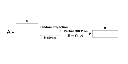
Figure 1: Use random projection to find $b$ pivots in each iteration.

Since Algorithm 2 is a left-looking algorithm, it’s much more efficient than DPSTRF.f when $k\ll n$. Numerical experiments also suggest that Algorithm 2 typically computes a better low-rank approximation than DPSTRF.f.

Updating formula for $B$: The formula for successively computing $B(\mbox{:,j+$\overline{b}$:n})$ for increasing j in Algorithm 2 is what makes Algorithm 2 so efficient. To derive it, we first compute $B=\Omega\,A$. Algorithm 2 then computes $b$ pivots based on a partial QRCP on $B$ and performs a block Cholesky step. To continue, Algorithm 2 need to compute a random projection on the corresponding Schur complement, which it does not compute directly. We can re-use the initial random matrix $\Omega$ and the corresponding random projection $B$ to compute a special random projection for the Schur complement.

After the necessary row and column swaps and the block Cholesky step, we can write the matrices $A$, and $\Omega$ as ${\displaystyle\left(\begin{array}[]{cc}L_{11}&\\ L_{21}&I\\ \end{array}\right)\left(\begin{array}[]{cc}L_{11}^{T}&L_{21}^{T}\\ &S_{2}\\ \end{array}\right)}$, and ${\displaystyle\left(\begin{array}[]{cc}\Omega_{1}&\Omega_{2}\\ \end{array}\right)}$, respectively. The column swapped $B$ can be written as

$${\displaystyle\left(\begin{array}[]{cc}B_{1}&B_{2}\\ \end{array}\right)=\left(\begin{array}[]{cc}\Omega_{1}&\Omega_{2}\\ \end{array}\right)\;\left(\begin{array}[]{cc}L_{11}&\\ L_{21}&I\\ \end{array}\right)\left(\begin{array}[]{cc}L_{11}^{T}&L_{21}^{T}\\ &S_{2}\\ \end{array}\right),}$$

which, in turn, implies a special random projection formula

$$\Omega_{2}\;S_{2}=B_{2}-\left(\begin{array}[]{cc}\Omega_{1}&\Omega_{2}\\ \end{array}\right)\left(\begin{array}[]{c}L_{11}\\ L_{21}\\ \end{array}\right)L_{21}^{T}.$$ (4)

We can compute the random projection $\Omega_{2}S_{2}$ for $S_{2}$ via the right hand side expression in equation (4), with $\Omega_{2}$ as the random matrix. Generalizing this consideration for all j results in the formula for computing $B(\mbox{:,j+$\overline{b}$:n})$ in Algorithm 2.

Complexity analysis: The most work of Algorithm 2 are computing the initial random projection matrix $B=\Omega A$ and updating pivoted block $A(\mbox{j:n,j+$\overline{b}$-1})$ for each $j$. Computing $B$ requires $O(n^{2}p)$ operations and updating all pivoted blocks requires $O(nk^{2})$ operations, leading to the overall complexity of $O(n^{2}p+nk^{2})$ operations. Note that if both $p\ll n$ and $k\ll n$, then the complexity is $O(n^{2}p)$, i.e., the dominant computation is in the overhead – computing $B=\Omega A$.

III-B Spectrum-revealing Cholesky factorization

Greedy pivoting strategies in DPSTRF.f and Algorithm 2 typically compute good quality low-rank approximations, but not always. Below we first discuss what low-rank approximations are possible based on diagonal pivoting alone, and then develop a swap strategy to modify the partial Cholesky factorization computed from Algorithm 2 to ensure such an approximation. With a slight abuse of notation, $\Pi$ in Theorem 1 denotes a permutation matrix. Recall that for any matrix $X$, $\left|\left|X\right|\right|_{2,1}$ is equal to the largest of the column norms of $X$, and $\left|\left|X\right|\right|_{\max}$ is equal to the largest entry of $X$ in absolute value.

Theorem 1.

Let $A\in{}\mathbb{R}^{n\times{}n}$ be symmetric positive definite with a partial Cholesky factorization for $k<n$:

$$\Pi^{T}A\Pi=LL^{T}+\left(\begin{array}[]{cc}0&0\\ 0&S\\ \end{array}\right)$$ (5)

$$\mbox{with }\quad L=\left(\begin{array}[]{c}L_{11}\\ \ell^{T}\\ L_{21}\\ \end{array}\right),\quad\mbox{and}\quad S=\left(\begin{array}[]{cc}\alpha&s^{T}\\ s&\widehat{S}\\ \end{array}\right),$$

where $L_{11}\in{}\mathbb{R}^{k\times{}k},\ell\in{}\mathbb{R}^{k\times{}1},L_{21}\in{}\mathbb{R}^{(n-k-1)\times{}k},\alpha{}\in{}\mathbb{R},s\in{}\mathbb{R}^{(n-k-1)\times{}1}$, and $\widehat{S}\in{}\mathbb{R}^{(n-k-1)\times{}(n-k-1)}$.

Assume that $\alpha=\left|\left|S\right|\right|_{\max}$ and that for a given $g>1$,

$$\frac{1}{\sqrt{\alpha}} \geq{}\frac{1}{\sqrt{g}}\left|\left|\left(\begin{array}[]{cc}L_{11}&\\ \ell^{T}&\sqrt{\alpha}\\ \end{array}\right)^{-1}\right|\right|_{2,1},$$ (8)

then there exists a $\tau\leq g(n-k)(k+1)$ such that for $1\leq j\leq k$

(9)

(10)

∎

If conditions on $\alpha$ hold, then Theorem 1 asserts that the matrix approximation error is at most a factor of $\tau$ away from being optimal in $2$-norm; and all the singular values of $L$ are at most a factor of $\sqrt{1+\tau}$ away from being optimal. In addition, for the largest singular values of $A$ where ${\displaystyle\frac{\lambda_{k+1}(A)}{\lambda_{j}(A)}\ll 1}$, the corresponding approximate singular values $\sigma_{j}(L)$ are very close to $\sqrt{\lambda_{j}(A)}$, the best possible for any rank $k$ approximation.

A partial Cholesky factorization of the form (5) is said to be Spectrum-revealing if it satisfies the conditions on $\alpha$ in Theorem 1. The singular value lower bound in relation (10) represents a unique feature in a Spectrum-revealing Cholesky (SRCH) factorization.

DPSTRF.f ensures the condition $\alpha=\left|\left|S\right|\right|_{\max}$ by performing diagonal pivoting, but may not satisfy condition (8), leading to potentially poor approximations.

Algorithm 3 is a randomized algorithm that efficiently computes a Spectrum-revealing Cholesky factorization. It initializes the permutation with Algorithm 2. If Algorithm 2 fails condition (8), Algorithm 3 makes additional randomized column and row swaps to ensure it. In the algorithm, we denote $\widehat{L}=\left(\begin{array}[]{cc}L_{11}&\\ \ell^{T}&\sqrt{\alpha}\\ \end{array}\right)$.

Algorithm 3 A randomized algorithm to compute an SRCH

Inputs:      Positive semidefinite $A\in{}\mathbb{R}^{n\times{}n}$;

               block size $b$; over-sampling size $p\geq b$;

               parameter $g>1$; approximate rank $k\ll n$.

Outputs:    Permutation vector ${\Pi}\in{}\mathbb{R}^{n}$; matrix $L$.

Initialize:   compute ${\Pi}$ and $L$ with Algorithm 2

Generate random $\Omega\in\mathcal{N}(0,1)^{d\times{}(k+1)}$

compute $\alpha={\bf max}{}(\text{diag(Schur complement)})$

while ${\displaystyle\frac{1}{\sqrt{\alpha}}<\frac{1}{\sqrt{gd}}\left\|\Omega{}\widehat{L}^{-1}\right\|_{2,1}}$ do

     $\imath={\bf argmax}_{1\leq{}i\leq{}k+1}\{i\text{th column norm of }\Omega{}\widehat{L}^{-1}\}$

     swap $\imath$-th and $(k+1)$-st columns and rows of $A$

     swap $\imath$-th and $(k+1)$-st entries in $\Pi$

     Givens-rotate $L$ back into lower-triangular form.

     compute $\alpha={\bf max}{}(\text{diag(Schur complement)})$

end while

Remarks: (1) We look through the diagonal of the Schur complement $S$ to find $\alpha$, thereby avoid computing $S$ itself. (2) The while loop in Algorithm 3 will eventually stop, after a finite number of swaps (bounded above by $O(n)$), leading to a permutation that satisfies conditions (8). However, at most a few swaps are enough in practice. (3) Each swap will make the $\imath$-th row out of the lower-triangular form. A round robin rotation is applied to the rows of $L$ and a quick sequence of Givens rotations are right multiplied to $L$ to restore its lower-triangular form. These Givens rotations are orthogonal and will cancel themselves out in the matrix product $LL^{T}$. (4) In some practical applications where more accurate singular values are desirable, one can compute an SRCH for a rank $\widehat{k}$ approximation $\widehat{L}\widehat{L}^{T}$ with $\widehat{k}>k$ and then SVD-truncate the matrix $\widehat{L}$ into a rank $k$ matrix $L$. This will lead to a rank-$k$ approximation $LL^{T}$ that satisfies

$$\lambda_{k+1}(A)\leq\left\|\Pi^{T}A\Pi-LL^{T}\right\|_{2}\leq\lambda_{k+1}(A)+\widehat{\tau}\lambda_{\widehat{k}+1}(A),$$

$$\lambda_{j}(A)\geq\sigma_{j}^{2}(L)\geq\frac{\lambda_{j}(A)}{1+\widehat{\tau}{\bf min}\left\{1,(1+\widehat{\tau})\frac{\lambda_{\widehat{k}+1}(A)}{\lambda_{j}(A)}\right\}},$$

for $1\leq j\leq k$ and scalar $\widehat{\tau}\leq g(n-\widehat{k})(\widehat{k}+1)$. Especially for rapidly decaying singular values, i.e., $\lambda_{\widehat{k}+1}(A)\ll\lambda_{k+1}(A)$, these bounds make $LL^{T}$ almost indistinguishable from the best possible, the SVD-truncated rank-$k$ approximation.

Complexity analysis: In addition to initialization, Algorithm 3 needs to repeatedly compute the diagonal of the Schur complement, which can be done in $O(k(n-k))$ operations. We need to swap the column with largest diagonal entry to the leading column and update the pivoted column, which needs a matrix-vector multiplication, costing another $O(k(n-k))$ operations. Then we need to compute $\Omega{}\widehat{L}^{-1}$ and the corresponding column norms, costing $O(dk^{2})$ operations. The algorithm stops if the while loop condition fails. Otherwise we need to swap the column with largest column norm in $\Omega{}\widehat{L}^{-1}$ and the leading column in the Schur complement. The Givens rotations needed to restore lower-triangular form in $L$ cost $O(nk)$ operations. In total, the cost of performing one swap in Algorithm 3 is $O(nk+dk^{2})$ operations. Assuming $k\ll{}n$, this cost becomes $O(nk)$, which is negligible compared to $O(n^{2}p)$, the cost of initialization (Algorithm 2).

IV Numerical experiments

Data and source code are available at following URL .

Section IV-A compares the run times of DPSTRF.f and SRCH to obtain a partial Cholesky factorization. Section IV-B compares the approximation effectiveness of low-rank approximations computed by DPSTRF.f and SRCH. Section IV-C compares DPSTRF.f and SRCH on a pathological matrix. Section IV-D and section IV-E compare SRCH with other pivoted Cholesky factorization based algorithms in a prediction problem and Gaussian process, respectively. All experiments are implemented on a laptop with a 2.7 GHz Intel Core i5 CPU and 8GB of RAM.

IV-A Run time comparison

We compare the run times of DPSTRF.f and SRCH on a kernel matrix of Combined Cycle Power Plant Data (CCPP) with size of $9568\times{}4$. We use RBF kernel $k(x_{i},x_{j})=\exp{}(-||x_{i}-x_{j}||_{2}^{2}/2\sigma^{2})$ and set $\sigma=1.0$. In SRCH, we choose $b=20$ and $p=30$. Run times are in Fig. 3.

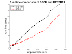
Figure 2: Run time comparison.

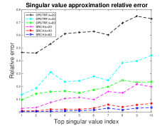
Figure 3: Top 10 singular value approximation relative error $\frac{\lambda_{j}(A)-\sigma_{j}^{2}(L)}{\lambda_{j}(A)}$.

DPSTRF.f is faster when approximate rank is small. This is because SRCH must compute the random projection $B=\Omega{}A$, which is an overhead. As approximate rank increases, SRCH becomes faster than DPSTRF.f as predicted.

IV-B Approximation effectiveness comparison

For the same kernel matrix used in section IV-A, we compare the approximation effectiveness of SRCH and DPSTRF.f with their low-rank approximations. We choose $k=20,40,60$, $b=20$ and $p=30$. Fig. 3 shows the approximation relative errors of the top $10$ eigenvalues of $A$. Although SRCH will be slower than DPSTRF.f because of the overhead cost of computing $B=\Omega{}A$, the approximation effectiveness of SRCH is much better than DPSTRF.f.

If we choose large approximate rank $k$, both SRCH and DPSTRF.f will provide very high quality low-rank approximations and there will be little difference between SRCH and DPSTRF.f in relative approximation errors for the leading singular values, but SRCH is significantly faster than DPSTRF.f, as Fig. 3 suggests.

IV-C A pathological example for Spectrum-revealing Cholesky factorization

The Kahan Matrix [14] is defined as $K_{n}=S_{n}C_{n}$, where

$${S_{n}={\textrm{\bf diag}}(1,s,\cdots,s^{n-1}),C_{n}=\left(\begin{array}[]{ccccc}1&-c&-c&\cdots&-c\cr&1&-c&\cdots&-c\cr&&1&\cdots&-c\cr&&&\ddots&\vdots\cr&&&&1\end{array}\right)}$$

for $s,c>0$ and $s^{2}+c^{2}\leq{}1$. The Kahan matrix is well-known for its peculiar behavior regarding estimation of conditioning and rank. Indeed, simple diagonal pivoting on the matrix $A\stackrel{{\scriptstyle def}}{{=}}K_{n}^{T}\,K_{n}$ will fail to produce a quality low-rank approximation.

We use DPSTRF.f and SRCH to compute a partial Cholesky factorization of $A$. We choose $c=0.285$, $s=\sqrt{0.9999-c^{2}}$, $n=130$ and $k=100$. We also set $g=1.5$, $d=b=20$ and $p=25$ in SRCH. Let the partial Cholesky factorization be $\Pi^{T}A\Pi=\left(\begin{array}[]{cc}L_{11}&\\ L_{21}&I_{n-k}\\ \end{array}\right)\left(\begin{array}[]{cc}L_{11}^{T}&L_{21}^{T}\\ &S\\ \end{array}\right)$ and we denote $L=\left(\begin{array}[]{c}L_{11}\\ L_{21}\\ \end{array}\right)$. Table I compares the approximation effectiveness of a few smallest singular values.

index	DPSTRF	SRCH
96	0.8855	0.9545
97	0.8739	0.9467
98	0.8594	0.9370
99	0.8390	0.9242
100	0.5820E-08	0.9055

TABLE I: Singular value approximation ratio $\frac{\sigma_{j}^{2}(L)}{\lambda_{j}(A)}$

The singular value ratios $\frac{\sigma_{j}^{2}(L)}{\lambda_{j}(A)}$ can never exceed $1$ for any approximation, but we would like them to be close to $1$ for a reliable spectrum-revealing Cholesky factorization. Table I demonstrates that DPSTRF.f failed to do so for the index $100$ singular value, whereas SRCH has succeeded for all singular values. SRCH required $2$ extra swaps to achieve this reliability. The run time of DPSTRF.f and SRCH are 5.060e-4 seconds and 1.359e-3 seconds respectively. SRCH is slower because the Kahan matrix in testing is small in dimension.

In typical machine learning and other applications of low-rank approximations, the extra swaps of Algorithm 3 are rarely needed. They serve as an insurance policy against occasional mistakes made by Algorithm 2. It is worth noting that the additional running time is negligible.

IV-D Cholesky factorization with side information (CSI)

[6] presents an algorithm that exploits side information in the prediction on unlabeled data with low-rank approximations for kernel matrices. To compute a low-rank approximation, this algorithm minimizes the objective function with a greedy strategy to incrementally select representative samples.

In this section we apply SRCH on the kernel matrix for a low-rank approximation without the benefit of side information, and make predictions on unlabeled data with this low-rank approximation. Details of the prediction formulas can be found in Section $6$ of [6].

We compare approximation effectiveness of the low-rank approximation, run time and prediction error on unlabeled data. We compare four methods: CSI decomposition with $40$ look-ahead steps, CSI decomposition with $80$ look-ahead steps, diagonal pivoted Cholesky without look-ahead and SRCH. The first three methods are from [6]. We test these four methods on handwritten digit (MNIST). We use RBF kernel $k(x_{i},x_{j})=\exp{}(-||x_{i}-x_{j}||_{2}^{2}/2\sigma^{2})$ and set $\sigma=1.0$. We set $b=50$ and $p=55$ in SRCH.

We choose $3000$ training samples, $3000$ testing samples and $k=200$. Fig. 5 and Fig. 5 show approximation effectiveness and prediction accuracy, respectively. There is a slight advantage of SRCH on both approximation effect and prediction accuracy. We define the approximation error as $\frac{trace(K-LL^{T})}{trace(K)}$.

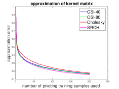
Figure 4: Approximation comparison.

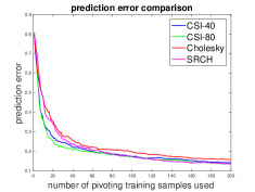
Figure 5: Prediction error comparison.

The more impressive improvement is in run time. Fig. 6 shows the run time comparison on the kernel matrix $K\in{}\mathbb{R}^{3000\times{}3000}$ for different approximate ranks $k$. SRCH is significantly faster than the other three methods.

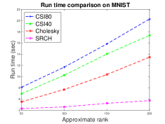
Figure 6: Run time comparison.

IV-E Gaussian process

Supervised learning is to learn input-output mappings using data. We assume the training data is $X\in\mathbb{R}^{n\times d}$, the target values of $X$ is $y\in\mathbb{R}^{n\times 1}$, the new data is $X^{*}\in\mathbb{R}^{n^{*}\times d}$ and the target values of $X^{*}$ is $y^{*}\in\mathbb{R}^{n^{*}\times 1}$. The goal is to predict $y^{*}$ given $X,y$ and $X^{*}$ [15]. In the Gaussian process, the prediction of $y^{*}$ involves a covariance function $\kappa(x,x^{\prime})$ where $x,x^{\prime}\in\mathbb{R}^{d}$. The covariance function can be used to construct the $n\times{}n$ covariance matrix $A$ with entries $A_{ij}=\kappa(x_{i},x_{j})$ where $x_{i}$ and $x_{j}$ are rows of $X$ and also the $n^{*}\times{}n$ cross covariance matrix $A^{*}$ where $A^{*}_{ij}=\kappa(x^{*}_{i},x_{j})$ where $x^{*}_{i}$ is the $i$th row of $X^{*}$. The prediction $\hat{y}^{*}$ for $y$ is given by the Gaussian process equation [16]

$$\hat{y}^{*}=A^{*}(\lambda I+A)^{-1}y$$ (13)

where $\lambda{}$ is a regularization parameter. It is not practical to solve equation (13) with large $n$ since the number of flops required is $O(n^{3})$. Therefore for large $n$ it is useful to develop approximate solutions to equation (13). We use the approximation formulas in [15] in this experiment.

We compute the Gaussian process on CCPP dataset with DPSTRF.f and SRCH. The training data matrix is of size $5000\times{}4$ and the testing data matrix is of size $4568\times{}4$. The covariance function is $\kappa(x_{i},x_{j})=\exp{}(-||x_{i}-x_{j}||_{2}^{2}/2\sigma^{2})$. We set $\lambda=5e-5$ and $\sigma=2.0$. In SRCH, we set $b=20$ and $p=25$. We compare the run time and mean squared prediction error in Fig. 8 and Fig. 8, respectively.

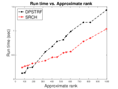
Figure 7: Run time comparison.

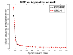
Figure 8: Prediction error comparison.

In Fig. 8, the run times of DPSTRF.f and SRCH intersect at around $250$. SRCH out-performs DPSTRF.f for larger approximate ranks. Fig. 8 demonstrates that while DPSTRF.f makes better predictions than SRCH for smaller approximate ranks $k$, they are not the range in which the best predictions are made. For larger $k$, SRCH provides slightly smaller prediction error than DPSTRF.f, as suggested in Fig. 8.

V Conclusion

In this work, we introduced spectrum-revealing Cholesky factorization (SRCH), a variant of the classical Cholesky factorization, for reliable low-rank matrix approximations of kernel matrices. We developed approximation error bounds as well as singular value approximation lower bounds for SRCH. We also developed an efficient and effective randomized algorithm for computing SRCH and demonstrated its efficiency and reliability against other Cholesky factorization based kernel methods on machine learning problems.

References

- [1] S. Fine and K. Scheinberg, “Efficient svm training using low-rank kernel representations,” The Journal of Machine Learning Research, vol. 2, pp. 243–264, 2002.
- [2] F. R. Bach and M. I. Jordan, “Kernel independent component analysis,” The Journal of Machine Learning Research, vol. 3, pp. 1–48, 2003.
- [3] C.-C. Chang and C.-J. Lin, “Libsvm: a library for support vector machines,” ACM Transactions on Intelligent Systems and Technology (TIST), vol. 2, no. 3, p. 27, 2011.
- [4] F. Pedregosa, G. Varoquaux, A. Gramfort, V. Michel, B. Thirion, O. Grisel, M. Blondel, P. Prettenhofer, R. Weiss, V. Dubourg et al., “Scikit-learn: Machine learning in python,” The Journal of Machine Learning Research, vol. 12, pp. 2825–2830, 2011.
- [5] E. Anderson, Z. Bai, C. Bischof, S. Blackford, J. Demmel, J. Dongarra, J. Du Croz, A. Greenbaum, S. Hammerling, A. McKenney et al., LAPACK Users’ guide. Siam, 1999, vol. 9.
- [6] F. R. Bach and M. I. Jordan, “Predictive low-rank decomposition for kernel methods,” in Proceedings of the 22nd international conference on Machine learning. ACM, 2005, pp. 33–40.
- [7] M. Gu, “Subspace iteration randomization and singular value problems,” SIAM Journal on Scientific Computing, vol. 37, no. 3, pp. A1139–A1173, 2015.
- [8] J. W. Demmel, L. Grigori, M. Gu, and H. Xiang, “Communication avoiding rank revealing qr factorization with column pivoting,” SIAM Journal on Matrix Analysis and Applications, vol. 36, no. 1, pp. 55–89, 2015.
- [9] P. Drineas, M. W. Mahoney, S. Muthukrishnan, and T. Sarlós, “Faster least squares approximation,” Numerische Mathematik, vol. 117, no. 2, pp. 219–249, 2011.
- [10] S. Wold, A. Ruhe, H. Wold, and W. Dunn, III, “The collinearity problem in linear regression. the partial least squares (pls) approach to generalized inverses,” SIAM Journal on Scientific and Statistical Computing, vol. 5, no. 3, pp. 735–743, 1984.
- [11] C. Lucas, “Lapack-style codes for level 2 and 3 pivoted cholesky factorizations,” LAPACK Working, 2004.
- [12] N. J. Higham, Accuracy and stability of numerical algorithms. Siam, 2002.
- [13] M. Gu and L. Miranian, “Strong rank revealing cholesky factorization,” Electronic Transactions on Numerical Analysis, vol. 17, pp. 76–92, 2004.
- [14] W. Kahan, “Numerical linear algebra,” Canadian Math. Bull, vol. 9, no. 6, pp. 757–801, 1966.
- [15] L. Foster, A. Waagen, N. Aijaz, M. Hurley, A. Luis, J. Rinsky, C. Satyavolu, M. J. Way, P. Gazis, and A. Srivastava, “Stable and efficient gaussian process calculations,” The Journal of Machine Learning Research, vol. 10, pp. 857–882, 2009.
- [16] C. K. Williams and C. E. Rasmussen, “Gaussian processes for machine learning,” the MIT Press, vol. 2, no. 3, p. 4, 2006.