Interplay of Wave Localization and Turbulence in Spin Seebeck Effect

Abstract

One of the most important discoveries in spintronics is the spin Seebeck effect (SSE) recently observed in both insulating and (semi-)conducting magnets. However, the very existence of the effect in transverse configuration is still a subject of current debates, due to conflicting results reported in different experiments. Present understanding of the SSE is mainly based on a particle-like picture with the local equilibrium approximation (LEA), i.e., spatially resolved temperature-field assumed to describe the system. In this work, we abandon the LEA to some extent and develop a wave theory to explain the SSE, by highlighting the interplay between wave localization and turbulence. We show that the emerging SSE with a sign change in the high/low-temperature regions is closely related to the extendedness of the spin wave that senses an average temperature of the system. On the one hand, ubiquitous disorders (or magnetic field gradients) can strongly suppress the transverse spin Seebeck effect (TSSE) due to Anderson (or Wannier-Zeeman) spin-wave localization. On the other hand, the competing wave turbulence of interacting magnons tends to delocalize the wave, and thus remarkably revives the TSSE before the magnon self-trapping. Our theory provides a promising route to resolve the heated debate on TSSE with a clear experiment scheme to test it in future spin caloritronic devices.

I Introduction

Spin Seebeck effect (SSE) refers to the generation of a spin voltage by temperature gradient in magnetic materials Uchida . There are two typical experimental configurations to measure the SSE: One is the transverse SSE (TSSE) Uchida ; Jaworski2 ; Uchida1 ; McLaughlin1 ; Huang1 ; Schmid1 ; Meier1 ; Bui1 ; Soldatov1 ; Meier in which a nonmagnetic metal bar is vertically placed on top of the magnetic strip. The other is the longitudinal SSE (LSSE) LSSE1 ; LSSE2 ; LSSE3 where the corresponding metal bar is connected to one end of the magnetic strip, and the thermal gradient is perpendicular to the magnetic$|$nonmagnetic interface. While the LSSE is less questionable, the existence of the TSSE is a subject of recent debates (see Table 1 for summary)

The present interpretation of SSE is mainly based on a “particle-like” theory Xiao ; Adachi2 ; Hiroto ; Jaworski1 pioneered by Sanders and Walton Sanders , assuming that both the magnon-magnon and phonon-phonon interactions are much stronger than the magnon-phonon coupling so that magnons and phonons form two coupled Boson gasses with different local temperatures Xiao ; Adachi2 . The local energy exchange rate between the two gasses is proportional to their temperature difference. However, the measured temperature difference between magnon and phonon is too small Agrawal to explain the TSSE. An alternative view relies on the phonon-drag mechanism Hiroto ; Jaworski1 that aims to explain the enhancement of the TSSE signal at low temperature. This mechanism should be important for a strong magnon-phonon interaction, which is not consistent with experimental evidences of relatively weak magnon-phonon coupling in large-scale transports in magnetic insulator Agrawal ; Guo1 .

Table 1: The table summarizes experimental results of the TSSE in ferro-(or ferri-)magnetic metals (FMs), semiconductors (FSCs), and insulators (FIs), as well as the length of the sample used in corresponding measurements. In these experiments, the length of the thin films $L$ ranges from 5 mm to 8 mm. Conventionally, the TSSE is detected through the inverse spin Hall effect in the adjacent heavy metal bar. Thus, in early experiments, the electric detections are inevitably mixed with the thermoelectric and magnetoelectric effects. A recent experiment McLaughlin1 reports the TSSE via a novel optical method.

Reports of TSSE	Length $L$ (mm)	Reports of no TSSE	Length $L$ (mm)
Uchida, K. et al Uchida (FM)	8	Huang, S. Y. et al Huang1 (FM)	5
Jaworski, C. M. et al Jaworski2 (FSC)	8	Schmid, M. et al Schmid1 (FM)	5
Uchida, K. et al Uchida1 (FI)	5	Meier, D. et al Meier1 (FM)	5
McLaughlin R. et al McLaughlin1 (FM)	5	Bui, C. T. et al Bui1 (FM)	5
		Soldatov, I. V. et al Soldatov1 (FSC)	5
		Meier, D. et al Meier (FI)	5

Two assumptions are often adopted in the particle-like theory: First, spin waves in ferromagnets are assumed to be extended although a typical “propagation length” of thermal magnons is also introduced phenomenologically in clean systems. However, inevitable material imperfections introduce disorders Sun1 ; Wesenberg1 , which may lead to the spin-wave Anderson localization Nowak . Meanwhile, the applied temperature gradient can generate a spatial dependence of the magnetic anisotropy Antropov ; Garad ; Hannes1 , so that local magnetic moments experience an inhomogeneous magnetic field which can result in a spin-wave Wannier-Zeeman localization Yan1 . Second, magnons are assumed to be in thermal equilibrium with the local surroundings such that a position-dependent magnon temperature is introduced, while the global system is still out of equilibrium. Nonetheless, this local equilibrium approximation (LEA) often leads to contradictions, e.g., the local temperature obtained by the kinetic method is different from that by the entropic approach Narayanan1 . Furthermore, the SSE should not require phonons for existence, just like its counterpart of normal Seebeck effect where phonon usually plays a bad role, and one tries to eliminate its effect. Thus, it is highly interesting and important to see whether one can understand the spin transport in the TSSE with neither the LEA nor the magnon-phonon coupling (at least not explicitly), which motivates us to revisit this outstanding issue and to propose a more general wave theory.

In this article, we use the stochastic Landau-Lifshitz-Gilbert (LLG) equation to describe the magnetization dynamics and to formulate the interplay between spin-wave localization and turbulence Nazarenko which captures the statistical property of large numbers of incoherent interacting magnons. The effects of phonons and other possible degrees of freedom such as electromagnetic radiations are to provide a stochastic magnetic field Andreas ; Photon and to establish a local temperature for electrons in the heavy-metal detecting bar. We consider the Y₃Fe₅O${}_{12}|$Pt (YIG$|$Pt) bilayer as the model system [see Fig. 1(a)]. We show that the TSSE is a consequence of the extendedness of spin waves and the temperature of nonequilibrium magnons is mode dependent. Three relevant length scales are identified: the localization length of spin waves $\xi$, the length of YIG film $L$, and the width of Pt contact $w$. Spread spin waves ($\xi\sim L$) can sense an average temperature of the system, and are therefore not in thermal equilibrium with electrons in the Pt contact. The TSSE is thus generated with a sign change in the high-/low-temperature regions, detected by the inverse spin Hall voltage. On the contrary, highly-localized spin waves ($\xi\sim w$) sense only the local bath temperature and are in thermal equilibrium with the itinerant electrons, leading to a strong suppression of the TSSE. Our idea is schematically shown in Fig. 2. Interestingly, we find that magnon-magnon interactions play remarkable roles in the spin transport: (i) At elevated temperature, spin-wave turbulence competes with the localization to make magnons more extended, and therefore revive the TSSE, and (ii) Magnon with a renormalized dispersion relation serves as the spin and heat carrier.

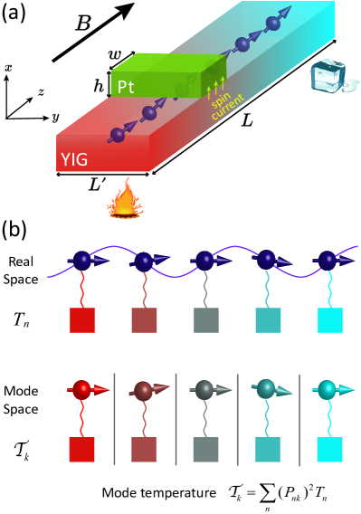
Figure 1: (a) Schematic plot of the YIG$|$Pt system, which includes a rectangle-shaped YIG with a Pt detect bar attached on its surface. A temperature gradient $\nabla T$ is applied in the quasi 1D system along $z-$direction. The net spin current is injected along the perpendicular direction with spatial distributions $j^{z}_{s,n}$, which is converted into an electric voltage by the inverse spin Hall effect. For arbitrary temperature profile $T_{n}$, $j^{z}_{s,n}\propto\left(\sum_{k}(P_{nk})^{2}\mathcal{T}_{k}-T_{n}\right)$, with $\mathcal{T}_{k}$ the mode temperature of magnons and $P_{nk}$ the spin wave function. (b) Temperature in both the real and the mode spaces. According to the principle of energy repartition at nonequilibrium steady states Yan1 , magnon at a given mode $k$ carries an energy $E_{k}=k_{B}\mathcal{T}_{k}$ with $\mathcal{T}_{k}=\sum_{n}(P_{nk})^{2}T_{n}$. Thus, the nonequilibrium system can be decomposed into “equilibrium” subsystems with well-defined spectrum temperature $\mathcal{T}_{k}$ in the normal-mode space.

Figure 2: The TSSE incorporates three physical situations: (i) For highly localized spin waves, $P_{nk}\simeq\delta_{nk}$, local magnons and electrons reach thermal equilibrium. In this case, $\mathcal{T}_{k}=T_{n}$, and no TSSE. (ii) For spread spin waves, magnons act globally such that the temperature for all modes is equal to the average temperature of the YIG, $\mathcal{T}_{k}=\bar{T}$. In this case, $j^{z}_{s,n}\propto\bar{T}-T_{n}$, and one should be able to observe the TSSE. (iii) Although the presence of disorders and field-gradients in disordered and/or anisotropic YIG tends to localize the spin wave, the intrinsic nonlinear nature of spin waves competes with the localizations. At moderate magnon-magnon interactions, spin waves can be delocalized, and thus revive the TSSE.

II Wave theory of TSSE

We model the YIG film by a two-dimensional (2D) Heisenberg ferromagnet of length $L$ and width $L^{\prime}$ with $N=LL^{\prime}/a^{2}$ local magnetic moments $\vec{S}_{\bm{n}}=S\vec{s}_{\bm{n}}$ where $S$ and $\vec{s}_{\bm{n}}$ are respectively the magnitude and the unit vector of the magnetic moment at site $\bm{n}=(n_{1},n_{2})$ (both $n_{1}$ and $n_{2}$ are integers, and $1\leq n_{1}\leq L^{\prime}/a$, $1\leq n_{2}\leq L/a$). Here $a=1.24~{}\hbox{nm}$ is the lattice constant. We start from the following Hamiltonian

$$\begin{gathered}\mathcal{H}=-\sum_{\langle\bm{n},\bm{n^{\prime}}\rangle}J\vec{s}_{\bm{n}}\cdot\vec{s}_{\bm{n^{\prime}}}+\sum_{\bm{n}}[D_{\bm{n}}(s^{z}_{\bm{n}})^{2}-BSs^{z}_{\bm{n}}],\end{gathered}$$ (1)

where $J>0$ is the nearest-neighbour exchange coupling constant and $D_{\bm{n}}$ is the local anisotropy constant. An external magnetic field $B\textbf{e}_{z}$ is applied to align the spin along $z-$direction [see Fig. 1 (a)]. Each spin is connected with a local Langevin thermal bath with temperature $T_{\bm{n}}$. To generate the spin current pumped from the YIG to Pt contact, we consider a linear temperature profile $T_{\bm{n}}=T_{0}+\Delta T(n_{2}a/L)$ in YIG with $T_{0}=300~{}\hbox{K}$ and $\Delta T=20~{}\hbox{K}$, without loss of generality.

The spin dynamics is then governed by the stochastic LLG equation Hoffman . For small spin fluctuations $\vec{s}_{\bm{n}}=(s^{x}_{\bm{n}},s^{y}_{\bm{n}},1)$ with $|s^{x,y}_{\bm{n}}|\ll 1$, the stochastic LLG equation reduces to the following stochastic dissipative discrete nonlinear Schrödinger equation for $\psi_{\bm{n}}\equiv s^{x}_{\bm{n}}+is^{y}_{\bm{n}}$

$$\begin{gathered}(i+\alpha)\dot{\psi}_{\bm{n}}=\dfrac{\gamma}{S}\left[J(\psi_{n_{1},n_{2}+1}+\psi_{n_{1},n_{2}-1})\right.\\ +J(\psi_{n_{1}+1,n_{2}}+\psi_{n_{1}-1,n_{2}})\left.-K_{\bm{n}}\psi_{\bm{n}}-\nu_{\bm{n}}|\psi_{\bm{n}}|^{2}\psi_{\bm{n}}\right]+\Theta_{\bm{n}},\end{gathered}$$ (2)

where $\alpha$ is the dimensionless Gilbert damping constant, $\gamma$ is the gyromagnetic ratio, and $K_{\bm{n}}=4J+BS-2D_{\bm{n}}$. An anisotropy-induced nonlinear four-magnon term, i.e., $-\nu_{\bm{n}}|\psi_{\bm{n}}|^{2}\psi_{\bm{n}}$ with $\nu_{\bm{n}}=D_{\bm{n}}$, is considered Kosevich . To model disorders and field gradients, we assume that the “on-site energy” $K_{\bm{n}}$ is random and uniformly distributed in the range of $[H_{0}+\epsilon n_{2}-W/2,H_{0}+\epsilon n_{2}+W/2]$ on top of a constant field $H_{0}$, with $\nu_{\bm{n}}=\nu=D$. Here $W$ and $\epsilon$ measure the strength of the disorder and the field gradient, respectively. In the following discussions, both $K_{\bm{n}}$ and $\nu$ are measured in the unit of $J$. Finite temperature effect is modeled by stochastic fields $\Theta_{\bm{n}}$ satisfying the fluctuation-dissipation theorem Brown1 , $\langle\Theta_{\bm{n}}(t)\Theta^{\ast}_{\bm{n}^{\prime}}(t^{\prime})\rangle=(4\alpha k_{B}T_{\bm{n}}\gamma/S)\delta_{n_{1}n^{\prime}_{1}}\delta_{n_{2}n^{\prime}_{2}}\delta(t-t^{\prime})$, where $k_{B}$ is the Boltzmann constant. We set $k_{B}=1$ such that the energy has the same unit with the temperature.

Disorders and inhomogeneous magnetic fields lead to the Anderson and Wannier-Zeeman localizations of spin waves, respectively. For $\nu=\epsilon=0$ and $W\neq 0$ (disorder only), the effective spin-wave Hamiltonian described by Eq. (2) belongs to the Gaussian orthogonal ensemble, and all spin waves are exponentially localized (Anderson localizations) Wang123 . While for $\nu=W=0$ and $\epsilon\neq 0$ (field gradient only), magnon states are periodic along $y-$direction and Wannier-Zeeman localized along $z-$direction with a localization length $\xi\simeq-a/[(\epsilon/J)\ln(\epsilon/J)]$ for $\epsilon\rightarrow 0$ Yan1 ; Kolovsky .

In the presence of a temperature gradient, the spin current is pumped into the Pt contact from the locally fluctuating spins in YIG, and its DC component at site $\bm{n}$ is given by Jiao1 ; Chen1

$$\begin{gathered}j^{z}_{s,\bm{n}}=-\dfrac{g^{\uparrow\downarrow}_{\text{eff}}\hbar}{4\pi}\Bigg{\langle}\text{Im}[\psi_{\bm{n}}\dot{\psi}_{\bm{n}}]\Bigg{\rangle},\end{gathered}$$ (3)

where $g^{\uparrow\downarrow}_{\text{eff}}$ is the effective spin mixing conductance at the interface, and $\langle\cdots\rangle$ denotes time average. Note that an accompanied spin current from the Pt contact back into YIG, which is proportional to the electron temperature $T_{e}$ at the Pt contact Foros , must be taken into account to obtain the net spin current. Disregarding the Kapitza interfacial heat resistance, the electrons at the Pt contact are in thermal equilibrium with the local heat bath, i.e., $T_{e}=T_{\bm{n}}$.

We first focus on the limit of (quasi) 1D spin chain ($n_{1}=1,n_{2}=n$) since analytical solutions of the problem are likely to obtain. We are then able to get the expression of the net interfacial spin current

$$\begin{gathered}j^{z}_{s,n}=\dfrac{g^{\uparrow\downarrow}_{\text{eff}}\hbar\gamma}{2\pi S}\left(\sum_{k}(P_{nk})^{2}\mathcal{T}_{k}-T_{n}\right),\end{gathered}$$ (4)

where $P_{nk}$ is the amplitude of wave function of the $k$th magnon mode at site $n$, and $\mathcal{T}_{k}\equiv\sum_{n}(P_{nk})^{2}T_{n}$ is the corresponding mode temperature under the bath temperature field $T_{n}=T_{0}+\Delta T(na/L)$. Detailed derivations are presented in the Appendix A. It reveals one of the main differences between the present wave theory and the popular particle-like one Xiao ; Adachi2 ; Hiroto ; Jaworski1 ; Sanders : Instead of introducing a position-dependent magnon temperature $T^{\text{Magnon}}_{n}$ using the LEA, we show that the temperature of non-equilibrium magnons is genuinely spectrum resolved as $\mathcal{T}_{k}$. The origin of TSSE then can be understood as follows: For extended spin waves with $\xi\simeq\infty$, they sense an average temperature of the whole system $\mathcal{T}_{k}=\bar{T}=\sum_{n}T_{n}a/L$, such that the magnon temperature in the high- (low-)$T$ region is lower (higher) than the bath temperature. The sign of TSSE is, therefore, opposite at the two ends. We emphasize that extended spin waves generally do not exist in disordered 1D spin chain since all spin waves are localized with a localization length $\xi\simeq(96J^{2}/W^{2})a$ kramer1 . However, as we illustrate later, as far as spin waves with long enough localized length ($\xi\sim L$ for spread spin waves), the magnons can still sense a mean temperature of the YIG. In the opposite limit, however, highly-localized magnons ($P_{nk}\sim\delta_{nk}$) inherit the same local temperature as the itinerant electrons in the Pt contact, and therefore cannot generate a net spin current, consistent with the second law of thermodynamics yuhua . Our arguments are qualitatively applicable to 2D, although the corresponding localization length is longer by a factor from 1 to 3 than 1D (see below).

III Anderson and Wannier-Zeeman localizations

To verify our analytical result, we numerically calculate the inverse spin Hall voltage $V_{H}(z)$ detected in the Pt contact of the YIG$|$Pt systems (See Methods VII.1 and Supplemental Material Sec. I supp ). In TSSE experiments, the typical width of the Pt contact $w=0.1~{}\hbox{mm}$, and the length of the YIG $L=5~{}\hbox{mm}$ (see Tables 1 and 2). In our simulations, we choose a fixed ratio $L/w=32$ close to the value in real measurements. A large-scale atomistic simulation of the YIG$|$Pt system for real TSSE experiments ($w\sim 10^{5}a$) is computationally too expensive. Instead, we perform the calculation by systematically increasing $w$ from $2a$ to $16a$ but fixing both the ratio of $\xi/w$ and the temperature difference $\Delta T$. Through this approach, we are able to quantitatively compare our simulations with the experimental results.

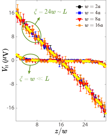
Figure 3: Inverse spin Hall voltage $V_{H}(z)$ for $w=2a,4a,8a,16a$ in 1D model. There are two bundles of curves, corresponding to the spread spin waves ($\xi=24w\sim L$) and the highly-localized spin waves ($\xi=w\ll L$). The localization length is tuned by the disorder strength through $\xi=(96J^{2}/W^{2})a$. Yellow dash curves are the theoretical formula Eq. (4).

We first calculate the quasi 1D case. Figure 3 displays the spatial distribution of $V_{H}(z)$ for $\xi=24w$ $(\sim L)$ and $\xi=w$ $(\ll L)$ with different Pt contact widths $w=2a,4a,8a,16a$, where symbols are numerical results. The localization lengths $\xi$ are tuned by the disorder strength $W$ via the formula $\xi=96J^{2}a/W^{2}$ kramer1 . It shows that the voltage solely depends on the ratio $\xi/w$, rather than the absolute value of the width of the Pt contact. Note that it is difficult to estimate or measure $\xi$ in real experiments, we consider the case $\xi=24w=2.4~{}\hbox{mm}$ (corresponding to $W/J=7\times 10^{-3}$, or $W=0.14~{}\hbox{K}$ in real unit) in the analytical calculation, and find that $V_{H}$ varies almost linearly with $z$ (see the upper yellow dashed curve in Fig. 3). The slope of $V_{H}(z)$ obtained both numerically and analytically is $6.4~{}\mu\hbox{V/mm}$, one order of magnitude larger than the experimental result ($0.5~{}\mu\hbox{V/mm}$) Uchida1 . Clearly, for the spread spin waves with localization lengths approaching the system size, we observe the sign change of the inverse spin Hall voltage at high-/low-temperature regimes, namely the TSSE. However, a shut down of the TSSE sets in when the spin wave localization length is of the same order of the width of the Pt contact, e.g., $\xi=w$, consistent with the theoretical analysis above. Numerical data compare well with the theoretical prediction (4) [see the lower bundle of curves in Fig. 3].

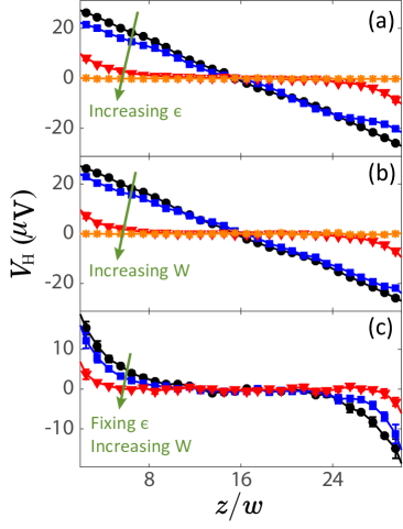
Figure 4: $V_{H}(z)$ for (a) $\epsilon=0,0.01,0.1,1$, and $W=0$ (Wannier-Zeeman localizations); (b) $\epsilon=0$, and $W=0,1,3,10$ (Anderson localizations); (c) $\epsilon=0.01$, and $W=0,1,3$ (both Wannier-Zeeman and Anderson localizations). The width of Pt contact is $w=4a$.

For tunable Wannier-Zeeman localization (zero disorder, finite field gradient) and Anderson localization (finite disorder, zero field gradient), the spatial dependence of the inverse spin Hall voltage $V_{H}(z)$ is shown in Figs. 4(a) and 4(b), respectively. In the calculations, we choose $w=4a$, without loss of generality, since it has been shown that TSSE only depends on the ratio $\xi/w$. In both cases, the TSSE is shown to be significantly suppressed by decreasing the localization length, and almost vanishes if $\xi<w$ [see the orange lines in Figs. 4(a) and 4(b)]. In real YIG$|$Pt systems under the temperature gradient, disorders and field gradients coexist, which should further suppress the TSSE. It is indeed the case as shown in Fig. 4(c).

Next, we proceed with the 2D case. In Fig. 5(a), we plot the $V_{H}$ versus the position $z$. It again shows that the magnitude of inverse spin Hall voltage is strongly suppressed by increasing the disorder, similar to what we observed in 1D system above. By comparing the results of 1D and 2D, cf. Fig. 4(b) and Fig. 5(a), we find that the magnitude of the TSSE in 2D is relatively larger than that in 1D (but still in the same order). This can be explained by the fact that the localization length in high dimension is usually larger than that in the low dimension, which indeed can be seen in Fig. 5(b) by evaluating the average participation numbers of both 1D and 2D systems [see Methods VII.2 for more details]. Moreover, we expect that the spin waves can be cooperatively localized in 2D system with even weaker disorders assisted by the field gradient (See Supplemental Material Sec. II supp ), just as the 1D results shown in Fig. 4(c). Our study thus quantitatively validates the role of spin-wave Anderson (Wannier-Zeeman) localization in TSSE, regardless of the system dimension.

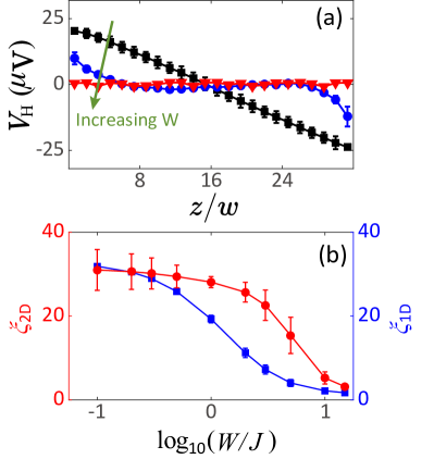
Figure 5: (a) Inverse spin Hall voltage $V_{H}(z)$ for $W=1$ (black squares), 10 (blue circles), and 15 (red triangles) in 2D model. The length and width of the 2D lattice are $L=64a$ and $L^{\prime}=24a$ (the ratio $L/L^{\prime}$ is close to the experiment value Uchida1 ). The width of the Pt contact is $w=2a$. (b) Average participation number (square root of participation number) $\xi_{1D}$ ($\xi_{2D}$) as a function of $W$ for 1D (2D) system. The system sizes are chosen as $L^{d}$ for $L=48a$ and $d=1,2$.

IV Wave turbulence

Remarkably, the spin-wave turbulence due to many-body interactions enriches the above picture because a large enough nonlinearity tends to delocalize magnons after a long run (reaching a steady state). There are three relevant energy scales: the average energy spacing $\overline{\delta\omega}$, the spectrum band-width $\Delta$, and the energy shift due to the magnon-magnon interaction $g\sim\nu|\psi_{n}|^{2}$. One expects three different regimes: (i) $g<\overline{\delta\omega}$ where the nonlinearity is not strong enough to cause the wave turbulence, and spin waves are localized; (ii) $\overline{\delta\omega}<g<\Delta$ where all spin waves are in turbulent states and delocalized; (iii) $\Delta<g$ where the nonlinearity is so strong that spin waves fall into the self-trapping region. To confirm this criterion, we study the spin wave spreading at $T=0~{}\hbox{K}$ in 1D system by numerically calculating the time evolution of the second-moment $\sigma_{2}(t)\equiv\langle\sum_{n}(n-\langle n\rangle)^{2}|\psi_{n}(t)|^{2}\rangle$ of an initial single-site excitation for different nonlinearities, shown in Fig. 6(a). Indeed, the spin waves undergo a sub-diffusive motion $\sigma_{2}\propto t^{\beta}$ for a strong nonlinearity $\nu=1$ while the Anderson localization occurs for $\nu=0$ and $0.001$. Our numerical data indicates $\beta=0.306\pm 0.002$, which is consistent with Ref. Pikovsky . For a very large nonlinearity $\nu=10$, spin waves are self-trapped.

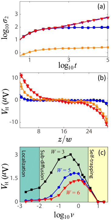
Figure 6: (a) Wave-packet second-moment $\log_{10}\sigma_{2}$ v.s. $\log_{10}t$ for $\nu=0$ (black squares), 0.01 (blue circles), 1 (red triangles), and 10 (orange stars) at $\epsilon=0$ and $W=3$. Values of $\log_{10}\sigma_{2}$ are averaged over time interval $\Delta(\log_{10}t)\simeq 0.1$. Purple dashed line is the linear fit of $\log_{10}\sigma_{2}=\beta\log_{10}t+\gamma$ with $\beta=0.306\pm 0.002$ and $\gamma=1.22\pm 0.01$. (b) Spatial distribution of $V_{H}$ for $\epsilon=0,W=3$, $\nu=0$ (black squares), 0.001 (blue circles), 0.1 (red triangles), and 1 (orange stars). (c) $V_{H}(z=4w)$ v.s. $\log_{10}\nu$ for $\epsilon=0$ under different disorder strengths. $w=4a$ is used in (b) and (c).

The TSSE then is expected to follow the predictions in the three different regions. Figure 6(b) shows the spatial dependence of inverse spin Hall voltage for a fixed disorder $W=3$ under different nonlinearities $\nu=0,0.001,0.1$ and $1$ in 1D. Clearly, strong nonlinearities ($\nu=0.1$ and 1) can significantly enhance the TSSE due to the delocalization of magnons, compared to the results of $\nu=0$ and $0.001$. Typically, the nonlinearity is about $\nu=0.001$ for pure YIG (see Table 2 in Appendix C). Thus, the YIG$|$Pt systems in most TSSE experiments belong to the Anderson localization phase, where the TSSE signals are too small to be observed. However, for the doped YIG (YBi)₃(FeGa)₅O₁₂ with high anisotropies novoselov , $\nu=0.84$ (or 16.8 K in real unit), one may expect a transition from the Anderson localization to the sub-diffusion, thus a giant enhancement of the TSSE. However, the TSSE is suppressed again by an ultrastrong nonlinearity due to the magnon self-trapping. Figure 6(c) shows the predicted three phases of TSSE.

Finally, we would like to point out that, at elevated temperature, the spin wave dispersion relation is shifted due to the nonlinearity. For extended spin waves, we are able to analytically calculate the dispersion of the renormalized mode due to the magnon-magnon interaction (See Appendix B for the derivation),

$$\begin{gathered}\tilde{\omega}_{k}=\omega_{k}+\dfrac{2\nu\gamma}{S}\sum^{N}_{p=1}\bar{n}_{p}/N,\end{gathered}$$ (5)

where $\bar{n}_{p}$ is the number of the $p$th normal magnon mode at steady states. Numerical results excellently agree with the analytical formula (5) (See Supplemental Material Sec. III supp ). For YIG at room temperature ($300~{}\hbox{K}$), we estimate the energy shift due to the renormalization as $0.536~{}\hbox{K}$, which can not be neglected since it is comparable to the temperature difference applied at the two ends of YIG in the TSSE experiment Uchida1 . Naturally, the renormalized spin wave should act as the carrier for both the heat and the spin currents in TSSE, which is numerically demonstrated in Supplemental Material Sec. III supp .

V Discussion

We would like to make a few more remarks before concluding this article. (i) In principle, our theory should hold for the SSE in both transverse and longitudinal configurations. (ii) The electric signal observed in TSSE experiments comes not only from SSE but inevitably also from other sources such as the anomalous Nernst effect Chien1 and the conventional Seebeck effect driven by thermal Hall current in ferromagnets, as well as the longitudinal SSE due to the local temperature differences between YIG and Pt bar. Although the TSSE signal is sensitive to spin-wave localization, other sources do not require delocalization of spin waves. Thus, one can experimentally separate a TSSE signal from other signals by applying (or not applying) a large field gradient along $z-$direction to switch off (on) TSSE signal through the Wannier-Zeeman localization. For the YIG$|$Pt system with $w=0.1~{}\hbox{mm}$, a magnetic field gradient $\epsilon=0.21~{}\hbox{T/mm}$ is able to switch off the TSSE response (see Methods VII.3). Taking into account the effect of both spin-wave Anderson and Wannier-Zeeman localizations, a much smaller field-gradient should be enough for that purpose. (iii) Interestingly, we note a long-range spin transport in disordered magnets recently reported in the amorphous YIG Wesenberg1 . The model studied here is microscopically relevant to such experiments. (iv) How to generalize the present study to 3D and antiferromagnets should be interesting subjects, and also poses both theoretical and numerical challenges.

VI Conclusion

In this work, we reveal the relationship between the spin-wave localization and the TSSE. By carefully tuning the localization length $\xi$ through either the Anderson or the Wannier-Zeeman mechanism, we are able to identify that spread spin waves ($\xi\sim L$) in a ferromagnetic insulator (YIG) and electrons in a non-magnetic heavy metal (Pt) generally are not at thermal equilibrium (except at one single point where there is no spin pumping), while highly localized spin waves ($\xi\sim w$) and electrons are always at thermal equilibrium. This naturally explains why spin current pumped from ferromagnetic insulator to the detecting bar reverses its direction at the high-/low-temperature side, and gives a route to understand why different experiments can show contradictory results. Furthermore, we show that the nonlinearity tends to delocalize spin waves in the weakly turbulent region and thus enhances the TSSE, but leads to spin wave self-trapping in the strongly turbulent region so that the TSSE is significantly suppressed again. Our theory provides a novel framework to understand the tantalizing spin Seebeck effect and to resolve the lingering debate on the very existence of the TSSE, with clear experiment scheme proposed to test it.

VII Methods

VII.1 Atomistic simulation of spin dynamics

We adopt the modified SBAB₂ method to numerically calculate the spin wave functions $\psi_{\bm{n}}(t)$ governed by Eq. (2). The SBAB₂ method is an effective scheme to simulate the time evolution of the discrete nonlinear Schrödinger equation. Conventionally, the dissipations and thermal fluctuations are not included in the SBAB₂ method (see Ref. Pikovsky and references therein). We generalize this method to include the thermal effect by using the Itô stochastic calculus, and numerically calculate the inverse spin Hall voltage by Eq. (3) (see Supplemental Material Sec. I supp ). The accuracy of the modified SBAB₂ method has been tested: We numerically reproduce the well-known energy equipartition for equilibrium systems ($\Delta T=0$), as well as the energy repartition Yan1 for systems at nonequilibrium steady states in Supplemental Material Sec. III supp .

VII.2 Participation numbers

To quantify the degree of localization of spin waves in finite-size disordered YIG, we numerically compute the participation number, defined as Wang123

$$\begin{gathered}PN(\omega)=\dfrac{1}{\sum_{\bm{n}}|\psi_{\bm{n}}(\omega)|^{4}},\end{gathered}$$ (6)

by exactly calculating the $\psi_{\bm{n}}(\omega)$ corresponding to an eigenfrequency $\omega$ at $T=0~{}\hbox{K}$. For a maximal spread (uniform) state, we have $\psi_{\bm{n}}=1/\sqrt{N}$ $\forall\bm{n}$ and $PN=N$; while for a maximal localized state (single site excitation), we have $PN=1$. Thus, a larger $PN$ indicates a less localized spin wave. We use the average participation number, $\xi_{1D}=(1/N)\sum_{\omega}PN(\omega)$ to measure the extendedness of spin waves in 1D systems; while for 2D systems, we use the square root of the average participation number, $\xi_{2D}=\sqrt{(1/N)\sum_{\omega}PN(\omega)}$.

VII.3 Estimation of the magnetic field gradient to switch off TSSE

For Wannier-Zeeman localization, the magnon eigenfunction is the Bessel function of the first kind with asymptotic localization length $\xi\simeq-a/[(\epsilon/J)\ln(\epsilon/J)]$ for $\epsilon\rightarrow 0$ in a quasi-1D spin chain Yan1 . When $\xi<w$, the TSSE signal is switched off. Typically, the width of the detecting metal contact is $0.1~{}\hbox{mm}$. To localize spin waves in such length scale through the Wannier-Zeeman mechanism, one needs the on-site energy $K=1.44~{}\hbox{K}$ at one end and $0$ at the other end, for instance. For a system of length $L=5~{}\hbox{mm}$, the required magnetic field gradient is $0.21~{}\hbox{T/mm}$.

Appendix A Analytical expression for magnon-induced spin injection in disordered YIG$|$Pt systems

By modelling the disordered YIG as a 1D spin chain, we are able to analytically derive the net spin current pumped from YIG into Pt contact. In the absence of the dissipation, thermal fluctuation, and nonlinearity, Eq. (2) reduces to

$$\begin{gathered}i\dot{\psi}_{n}=\mathcal{H}_{0}\psi_{n}=\dfrac{\gamma}{S}[J(\psi_{n+1}+\psi_{n-1})-K_{n}\psi_{n}]\\ =-\omega_{k}\psi_{n},\end{gathered}$$ (7)

where $\omega_{k}$ is the frequency of the linear Hamiltonian $\mathcal{H}_{0}$, and $k$ labels the mode index. $\mathcal{H}_{0}$ can be diagonalized by an orthogonal matrix $P$, i.e., an expansion of $\psi_{n}$ into its mode space $\psi_{n}=\sum_{k}P_{nk}\phi_{k}$. When taking the thermal noise $\Theta_{n}$ into account, we have

$$\begin{gathered}(i+\alpha)\dot{\phi}_{k}=-\omega_{k}\phi_{k}+\Lambda_{k},\end{gathered}$$ (8)

where $\Lambda_{k}=\sum_{n}P_{nk}\Theta_{n}$. The DC component of spin current pumped from YIG to Pt can be calculated by Eq. (3)

$$\begin{gathered}j^{z}_{s,n}=-\dfrac{g^{\uparrow\downarrow}_{\text{eff}}\hbar}{4\pi}\text{Im}\left[\sum_{kk^{\prime}}P_{nk}P_{nk^{\prime}}\Bigg{\langle}\phi_{k}\dot{\phi}_{k^{\prime}}\Bigg{\rangle}\right],\end{gathered}$$ (9)

where $\langle\cdots\rangle$ represents the time averaging. $\langle\phi_{k}\dot{\phi}_{k^{\prime}}\rangle$ can be obtained by Eq. (8)

$$\begin{gathered}\langle\phi_{k}\dot{\phi}^{\ast}_{k^{\prime}}\rangle=\dfrac{i+\alpha}{1+\alpha^{2}}\left(-\omega_{k^{\prime}}\langle\phi_{k}\phi^{\ast}_{k^{\prime}}\rangle+\langle\Lambda^{\ast}_{k^{\prime}}\phi_{k}\rangle\right).\end{gathered}$$ (10)

For most TSSE experiments, the time scale of the dynamics of magnetizations $\tau_{m}$ is much longer than the time scale of the noisy environment $\tau_{n}$ such that $\Lambda^{\ast}_{k^{\prime}}$ and $\phi_{k}$ can be treated as independent variables. Thus, the second term in the right-hand side of Eq. (10) vanishes,

$$\begin{gathered}\langle\Lambda^{\ast}_{k^{\prime}}\phi_{k}\rangle=\langle\Lambda^{\ast}_{k^{\prime}}\rangle\langle\phi_{k}\rangle=0.\end{gathered}$$ (11)

To evaluate the first term of Eq. (10), we integrate Eq. (8) from $t$ to $t+\tau$ with $\tau_{n}\ll\tau\ll\tau_{m}$,

$$\begin{gathered}\phi_{k}(t+\tau)=\phi_{k}(t)+(i-\alpha)\omega_{k}\phi_{k}(t)\tau\\ -(i-\alpha)\int^{t+\tau}_{t}\Lambda_{k}(t_{1})dt_{1}.\end{gathered}$$ (12)

Thus, we have

$$\begin{gathered}\dfrac{d\langle\phi_{k}\phi^{\ast}_{k^{\prime}}\rangle}{dt}=-\dfrac{1}{1+\alpha^{2}}\left[(\alpha(\omega_{k}+\omega_{k^{\prime}})\right.\\ \left.+i(\omega_{k}-\omega_{k^{\prime}}))\langle\phi_{k}\phi^{\ast}_{k^{\prime}}\rangle+4\alpha k_{B}\gamma\mathcal{T}_{kk^{\prime}}/(S)\right],\end{gathered}$$ (13)

where $\mathcal{T}_{kk^{\prime}}=\sum_{n}P_{nk}P_{nk^{\prime}}T_{n}$. At steady state $d\langle\phi_{k}\phi^{\ast}_{k^{\prime}}\rangle/dt=0$,

$$\begin{gathered}\langle\phi_{k}\phi^{\ast}_{k^{\prime}}\rangle=\dfrac{4\alpha k_{B}\mathcal{T}_{kk^{\prime}}\gamma}{[\alpha(\omega_{k}+\omega_{k^{\prime}})+i(\omega_{k}-\omega_{k^{\prime}})]S}.\end{gathered}$$ (14)

Substituting Eq. (14) into Eq. (9), we obtain the expression of the net spin current,

$$\begin{gathered}j^{z}_{s,n}=\dfrac{2\alpha^{2}g^{\uparrow\downarrow}_{\text{eff}}\hbar\gamma}{\pi(1+\alpha^{2})S}\sum_{kk^{\prime}}P_{nk}P_{nk^{\prime}}\\ \times\dfrac{k_{B}(\mathcal{T}_{kk^{\prime}}-T_{n})\omega_{k}\omega_{k^{\prime}}}{\alpha^{2}(\omega_{k}+\omega_{k^{\prime}})^{2}+(\omega_{k}-\omega_{k^{\prime}})^{2}},\end{gathered}$$ (15)

where we include the Johnson-Nyquist noise generated in the Pt contact that is proportional to the electron temperature $T_{e}$, equal to the local temperature of the thermal bath. Disregarding the Kapitza interface heat resistance, the temperature of YIG is continuous over the interface, and $T_{e}=T_{n}$. For YIG with a small Gilbert damping $\alpha=10^{-4}$, only the diagonal terms in Eq. (15) contribute to the net spin current,

$$\begin{gathered}j^{z}_{s,n}=\dfrac{g^{\uparrow\downarrow}_{\text{eff}}\hbar\gamma}{2\pi S}k_{B}\left(\sum_{k}(P_{nk})^{2}\mathcal{T}_{k}-T_{n}\right),\end{gathered}$$ (16)

where $\mathcal{T}_{k}=\sum_{n}(P_{nk})^{2}T_{n}$ can be regarded as the temperature of the $k$th mode. Eq. (16) is Eq. (4) in the main text.

The net spin current $j^{z}_{s,n}$ pumped from the YIG into the Pt contact can be detected by the inverse spin Hall effect. The net spin current at site $n$ gives rise to a DC Hall current $j^{y}_{n}$,

$$\begin{gathered}j^{y}_{n}=\theta_{H}\dfrac{2e}{\hbar}j^{z}_{s,n},\end{gathered}$$ (17)

where $\theta_{H}$ is the inverse Hall angle. The length and width of the Pt contact are $L^{\prime}$ and $w$, respectively. The electric voltage over the two transverse ends of the Pt contact with position $z$ can be calculated by

$$\begin{gathered}V_{H}(z/w)=\dfrac{2\rho eL^{\prime}\theta_{H}}{A\hbar}\overline{j}^{z}_{s}(z/w).\end{gathered}$$ (18)

Here $\rho$ is the resistivity of the Pt contact, and $A$ is the contact area. $\overline{j}^{z}_{s}(z/w)$ is the mean net spin current pumped into the Pt contact.

Appendix B Renormalized dispersion relation

In the mode space of 1D model, Eq. (2) reads

$$\begin{gathered}(i+\alpha)\dot{\phi}_{k}=-\omega_{k}\phi_{k}\\ -\dfrac{\nu\gamma}{S}\sum_{k_{1}k_{2}k_{3}}I_{kk_{1}k_{2}k_{3}}\phi_{k_{1}}\phi^{\ast}_{k_{2}}\phi_{k_{3}}+\Lambda_{k},\end{gathered}$$ (19)

where $I_{kk_{1}k_{2}k_{3}}=\sum_{n}P_{nk}P_{nk_{1}}P_{nk_{2}}P_{nk_{3}}$ represents the coupling between different spin-wave modes due to the nonlinearity. To investigate the nonlinear effect, we integrate Eq. (19) from $t$ to $t+\tau$ with $\tau_{n}\ll\tau\ll\tau_{m}$

$$\begin{gathered}\phi_{k}(t+\tau)=\phi_{k}(t)+(i-\alpha)\omega_{k}\phi_{k}(t)\tau\\ +(i-\alpha)\dfrac{\nu\gamma}{S}\sum_{k_{1}k_{2}k_{3}}I_{kk_{1}k_{2}k_{3}}\phi_{k_{1}}\phi^{\ast}_{k_{2}}\phi_{k_{3}}\\ -(i-\alpha)\int^{t+\tau}_{t}\Lambda_{k}(t_{1})dt_{1}.\end{gathered}$$ (20)

Then, we are able to find the time evolution equation of the mean number of the $k$th mode, $n_{k}=\langle\phi_{k}\phi^{\ast}_{k}\rangle$,

$$\begin{gathered}\dot{n}_{k}=-2\alpha\omega_{k}n_{k}+4\alpha k_{B}\mathcal{T}_{k}\gamma/S\\ -2(\nu\gamma/S)\sum_{k_{1}k_{2}k_{3}}I_{kk_{1}k_{2}k_{3}}\text{Re}\left[(\alpha-i)\langle\phi^{\ast}_{k}\phi_{k_{1}}\phi^{\ast}_{k_{2}}\phi_{k_{3}}\rangle\right].\end{gathered}$$ (21)

We apply the fixed boundary conditions at two ends such that the number of spins reduces to $N-1$ effectively. The eigenvalues of the linear Hamiltonian $\mathcal{H}_{0}$ are

$$\begin{gathered}\omega_{k}=2(J\gamma/S)[1-\cos(k\pi/N)],\end{gathered}$$ (22)

and the eigenfunctions are

$$\begin{gathered}P_{nk}=\sqrt{2/N}\sin(nk\pi/N),n=1,2,\cdots,N-1.\end{gathered}$$ (23)

Under the resonant condition, say $k=k_{1}$ and $k_{2}=k_{3}$, the coupling integral reads

$$\begin{gathered}I_{kk_{1}k_{2}k_{3}}=\left\{\begin{array}[]{c}1/N\text{, for }k\neq k_{2}\text{ or }N-k_{2}\\ \\ 3/(2N)\text{, for }k=k_{2}\text{ or }N-k_{2}\\ \end{array}\right..\end{gathered}$$ (24)

For a moderate nonlinearity, the number of magnons approximately follows the Gaussian distribution. By using Wick’s theorem, we have

$$\begin{gathered}\langle\phi_{k}\phi^{\ast}_{k}\phi_{k}\phi^{\ast}_{k}\rangle=\langle\phi_{k}\phi^{\ast}_{k}\rangle\langle\phi_{k}\phi^{\ast}_{k}\rangle+\langle\phi^{\ast}_{k}\phi_{k}\rangle\langle\phi^{\ast}_{k}\phi_{k}\rangle.\end{gathered}$$ (25)

Thus, the nonlinear term in Eq. (21) reads

$$\begin{gathered}\text{Re}\left[\dfrac{4\nu\tau}{i+\alpha}\sum_{p}I_{kkpp}\langle\phi^{\ast}_{k}\phi_{k}\phi_{p}\phi_{p}\rangle\right]\\ =\dfrac{4\nu\tau\alpha}{N}\left(\sum_{p}n_{p}+2n_{k}+\dfrac{1}{2}n_{N-k}\right)n_{k}.\end{gathered}$$ (26)

In the thermodynamic limit, i.e., $N\rightarrow\infty$,

$$\begin{gathered}\dot{n}_{k}=-2\alpha\omega_{k}n_{k}+\dfrac{\gamma}{S}\left[4\alpha k_{B}\mathcal{T}_{k}-4\nu\alpha\left(\sum^{N}_{p=1}n_{p}/N\right)n_{k}\right].\end{gathered}$$ (27)

Equation (27) demonstrates three important features: (i) For extended spin waves, every mode interacts with all the other modes. (ii) The energy repartition for nonequilibrium steady states, i.e., $E_{k}=\bar{n}_{k}\tilde{\omega}_{k}S/(2\gamma)=k_{B}\mathcal{T}_{k}$ with $\bar{n}_{k}\equiv n_{k}(t\rightarrow\infty)$, is exactly satisfied by the renormalized mode Eq. (5). Thus, the nonlinearity makes a mode-independent frequency shift $\Delta\omega=\tilde{\omega}_{k}-\omega_{k}$. The renormalized dispersion shifts upward (downward) for a positive (negative) $\nu$; (iii) The steady distribution $\bar{n}_{k}$ may go to infinite for a strong enough attractive magnon-magnon interaction ($\nu<0$), and leads to an instability.

Appendix C Parameters for the YIG$|$Pt system

Table 2: Materials parameters.

YIG
Quantity	Values	References
Gyromagnetic ratio $\gamma$	$1.76\times 10^{11}~{}\hbox{rad}/\hbox{Ts}$
Gilbert damping $\alpha$	$10^{-4}$	Kajiwara1
Saturation magnetization $4\pi S/a^{3}$	$1.4\times 10^{5}~{}\hbox{A/m}$	Kajiwara1
Exchange energy $J$	$20~{}\hbox{K}$	Shinozaki1 ; Xie1
Nonlinearity $\nu$	$0.02~{}\hbox{K}$	Hannes1
Mixing conductance $g^{\uparrow\downarrow}_{\text{eff}}/A$ ($A$ the contact area)	$1\times 10^{11}\hbox{cm}^{-2}$	Uchida1
External magnetic field $B$	$0.32~{}\hbox{T}$	Uchida1
Pt contact
Quantity	Values	References
Hall angle $\theta_{H}$	0.00037	Kimura1
Resistance $\rho$	$1\times 10^{-6}~{}\Omega\hbox{m}$	Uchida1
Geometry $L^{\prime}\times w\times h$	$4~{}\hbox{mm}\times 0.1~{}\hbox{mm}\times 15~{}\hbox{nm}$	Uchida1

References

- (1) K. Uchida, S. Takahashi, K. Harii, J. Ieda, W. Koshibae, K. Ando, S. Maekawa, and E. Saitoh, Observation of the Spin Seebeck Effect, Nature (London) 455, 778 (2008).
- (2) C. M. Jaworski, J. Yang, S. Mack, D.D. Awschalom, J.P. Heremans, and R.C. Myers, Observation of the Spin Seebeck Effect in a Ferromagnetic Semiconductor, Nat. Mater. 9, 898 (2010).
- (3) K. Uchida, J. Xiao, H. Adachi, J. Ohe, S. Takahashi, J. Ieda, T. Ota, Y. Kajiwara, H. Umezawa, H. Kawai, G.E.W. Bauer, S. Maekawa, and E. Saitoh, Spin Seebeck Insulator, Nat. Mater. 9, 894 (2010).
- (4) R. McLaughlin, D. Sun, C. Zhang, M. Groesbeck, and Z.V. Vardeny, Optical detection of transverse spin-Seebeck effect in permalloy film using Sagnac interferometer microscopy, Phys. Rev. B 95, 180401(R) (2017).
- (5) S.Y. Huang, W.G. Wang, S.F. Lee, J. Kwo, and C.L. Chien, Intrinsic Spin-Dependent Thermal Transport, Phys. Rev. Lett. 107, 216604 (2011).
- (6) M. Schmid, S. Srichandan, D. Meier, T. Kuschel, J.-M. Schmalhorst, M. Vogel, G. Reiss, C. Strunk, and C.H. Back, Transverse Spin Seebeck Effect versus Anomalous and Planar Nernst Effects in Permalloy Thin Films, Phys. Rev. Lett. 111, 187201 (2013).
- (7) D. Meier, D. Reinhardt, M. Schmid, C.H. Back, J.-M. Schmalhorst, T. Kuschel, and G. Reiss, Influence of heat flow directions on Nernst effects in Py/Pt bilayers, Phys. Rev. B 88, 184425 (2013).
- (8) C.T. Bui and F. Rivadulla, Anomalous and planar Nernst effects in thin films of the half-metallic ferromagnet La2/3Sr1/3MnO3, Phys. Rev. B 90, 100403(R) (2014).
- (9) I.V. Soldatov, N. Panarina, C. Hess, L. Schultz, and R. Schäfer, Thermoelectric effects and magnetic anisotropy of Ga1-xMnxAs thin films, Phys. Rev. B 90, 104423 (2014).
- (10) D. Meier, D. Reinhardt, M. van Straaten, C. Klewe, M. Althammer, M. Schreier, S.T.B. Goennenwein, A. Gupta, M. Schmid, C.H. Back, J.-M. Schmalhorst, T. Kuschel, and G. Reiss, Longitudinal spin Seebeck effect contribution in transverse spin Seebeck effect experiments in Pt/YIG and Pt/NFO, Nat. Commun. 6, 8211 (2015).
- (11) K. Uchida, H. Adachi, T. Ota, H. Nakayama, S. Maekawa, and E. Saitoh, Observation of longitudinal spin-Seebeck effect in magnetic insulators, Appl. Phys. Lett. 97, 172505 (2010).
- (12) M. Weiler, M. Althammer, F.D. Czeschka, H. Huebl, M.S. Wagner, M. Opel, I.-M. Imort, G. Reiss, A. Thomas, R. Gross, and S.T.B. Goennenwein, Local Charge and Spin Currents in Magnetothermal Landscapes, Phys. Rev. Lett. 108, 106602 (2012).
- (13) K. Uchida, T. Kikkawa, A. Miura, J. Shiomi, and E. Saitoh, Quantitative Temperature Dependence of Longitudinal Spin Seebeck Effect at High Temperatures, Phys. Rev. X 4, 041023 (2014).
- (14) J. Xiao, G.E.W. Bauer, K. Uchida, E. Saitoh, and S. Maekawa, Theory of magnon-driven spin Seebeck effect, Phys. Rev. B 81, 214418 (2010).
- (15) H. Adachi, J. Ohe, S. Takahashi, and S. Maekawa, Linear-response theory of spin Seebeck effect in ferromagnetic insulators, Phys. Rev. B 83, 094410 (2011).
- (16) H. Adachi, K. Uchida, E. Saitoh, J. Ohe, S. Takahashi, and S. Maekawa, Gigantic enhancement of spin Seebeck effect by phonon drag, Appl. Phys. Lett. 97, 172505 (2010).
- (17) C.M. Jaworski, J. Yang, S. Mack, D.D. Awschalom, R.C. Myers, and J.P. Heremans, Spin-Seebeck Effect: A Phonon Driven Spin Distribution, Phys. Rev. Lett. 106, 186601 (2011).
- (18) D.J. Sanders and D. Walton, Effect of magnon-phonon thermal relaxation on heat transport by magnons, Phys. Rev. B 15, 1489 (1977).
- (19) M. Agrawal, V.I. Vasyuchka, A.A. Serga, A.D. Karenowska, G.A. Melkov, and B. Hillebrands, Direct Measurement of Magnon Temperature: New Insight into Magnon-Phonon Coupling in Magnetic Insulators, Phys. Rev. Lett. 111, 107204 (2013).
- (20) E. Guo, J. Cramer, A. Kehlberger, C.A. Ferguson, D.A. MacLaren, G. Jakob, and M. Kläui, Influence of Thickness and Interface on the Low-Temperature Enhancement of the Spin Seebeck Effect in YIG Films, Phys. Rev. X 6, 031012 (2016).
- (21) Y. Sun, H. Chang, M. Kabatek, Y.-Y. Song, Z. Wang, M. Jantz, W. Schneider, M. Wu, E. Montoya, B. Kardasz, B. Heinrich, S.G.E. te Velthuis, H. Schultheiss, and A. Hoffmann, Damping in Yttrium Iron Garnet Nanoscale Films Capped by Platinum, Phys. Rev. Lett. 111, 106601 (2013).
- (22) D. Wesenberg, T. Liu, D. Balzar, M. Wu, and B.L. Zink, Long-distance spin transport in a disordered magnetic insulator, Nat. Phys. 13, 987 (2017).
- (23) M. Evers, C.A. Müller, and U. Nowak, Spin-wave localization in disordered magnets, Phys. Rev. B 92, 014411 (2015).
- (24) V.P. Antropov, V.N. Antonov, L.V. Bekenov, A. Kutepov, and G. Kotliar, Magnetic anisotropic effects and electronic correlations in MnBi ferromagnet, Phys. Rev. B 90, 054404 (2014).
- (25) H. Garad, F. Fettar, F. Gay, Y. Joly, S. Auffret, B. Rodmacq, B. Dieny, and L. Ortega, Temperature Variation of Magnetic Anisotropy in Pt/Co/AlOx Trilayers, Phys. Rev. Applied 7, 034023 (2017).
- (26) H. Maier-Flaig, S. Klingler, C. Dubs, O. Surzhenko, R. Gross, M. Weiler, H. Huebl, and S.T.B. Goennenwein, Temperature-dependent magnetic damping of yttrium iron garnet spheres, Phys. Rev. B 95, 214423 (2017).
- (27) P. Yan, G.E.W. Bauer, and H. Zhang, Energy repartition in the nonequilibrium steady state, Phys. Rev. B 95, 024417 (2017).
- (28) K.R. Narayanan and A.R. Srinivasa, Shannon-entropy-based nonequilibrium “entropic” temperature of a general distribution, Phys. Rev. E 85, 031151 (2012).
- (29) Advances in Wave Turbulence, edited by V. Shrira and S. Nazarenko (World Scientific Publishing Company, Singapore, 2013).
- (30) A. Rückriegel and P. Kopietz, Rayleigh-Jeans Condensation of Pumped Magnons in Thin-Film Ferromagnets, Phys. Rev. Lett. 115, 157203 (2015).
- (31) M.C. Hickey and J.S. Moodera, Origin of Intrinsic Gilbert Damping, Phys. Rev. Lett. 102, 137601 (2009).
- (32) S. Hoffman, K. Sato, and Y. Tserkovnyak, Landau-Lifshitz theory of the longitudinal spin Seebeck effect, Phys. Rev. B 88, 064408 (2013).
- (33) A.M. Kosevich, B.A. Ivanov, and A.S. Kovalev, Magnetic Solitons, Physics Reports 194, 117 (1990).
- (34) W.F. Brown, Jr., Thermal Fluctuations of a Single-Domain Particle, Phys. Rev. 130, 1677 (1963).
- (35) C. Wang, Y. Su, Y. Avishai, Y. Meir, and X.R. Wang, Band of Critical States in Anderson Localization in a Strong Magnetic Field with Random Spin-Orbit Scattering, Phys. Rev. Lett. 114, 096803 (2015).
- (36) A.R. Kolovsky, Interplay between Anderson and Stark Localization in 2D Lattices, Phys. Rev. Lett. 101, 190602 (2008).
- (37) H. Jiao and G.E.W. Bauer, Spin Backflow and ac Voltage Generation by Spin Pumping and the Inverse Spin Hall Effect, Phys. Rev. Lett. 110, 217602 (2013).
- (38) K. Chen and S. Zhang, Spin Pumping in the Presence of Spin-Orbit Coupling, Phys. Rev. Lett. 114, 126602 (2015).
- (39) Jørn Foros, Arne Brataas, Yaroslav Tserkovnyak, and Gerrit E. W. Bauer, Magnetization Noise in Magnetoelectronic Nanostructures, Phys. Rev. Lett. 95, 016601 (2005).
- (40) B. Kramer and A. MacKinnon, Localization: theory and experiment, Reports on Progress in Physics 56, 1469 (1993).
- (41) Y.H. Shen, X.S. Wang, and X.R. Wang, Thermal spin current and spin accumulation at ferromagnetic insulator/nonmagnetic metal interface, Phys. Rev. B 94, 014403 (2016).
- (42) See Supplemental Material at http://link.aps.org/supplemental.
- (43) Y. Kajiwara, K. Harii, S. Takahashi, J. Ohe, K. Uchida, M. Mizuguchi, H. Umezawa, H. Kawai, K. Ando, K. Takanashi, S. Maekawa, and E. Saitoh, Transmission of electrical signals by spin-wave interconversion in a magnetic insulator, Nature (London) 464, 262 (2010).
- (44) S.S. Shinozaki, Specific Heat of Yttrium Iron Garnet from 1.5∘ to 4.2∘K, Phys. Rev. 122, 388 (1961).
- (45) L.-S. Xie, G.-X. Jin, L. He, G.E.W. Bauer, J. Barker, and K. Xia, First-principles study of exchange interactions of yttrium iron garnet, Phys. Rev. B 95, 014423 (2017).
- (46) T. Kimura, Y. Otani, T. Sato, S. Takahashi, and S. Maekawa, Room-Temperature Reversible Spin Hall Effect, Phys. Rev. Lett. 98, 156601 (2007).
- (47) A.S. Pikovsky and D.L. Shepelyansky, Destruction of Anderson Localization by a Weak Nonlinearity, Phys. Rev. Lett. 100, 094101 (2008).
- (48) K.S. Novoselov, A.K. Geim, S.V. Dubonos, E.W. Hill, and I.V. Grigorieva, Subatomic movements of a domain wall in the Peierls potential, Nature (London) 426, 812 (2003).
- (49) S.Y. Huang, X. Fan, D. Qu, Y.P. Chen, W.G. Wang, J. Wu, T.Y. Chen, J.Q. Xiao, and C.L. Chien, Transport Magnetic Proximity Effects in Platinum, Phys. Rev. Lett. 109, 107204 (2012).