Prospects of reaching the quantum regime in Li-Yb⁺ mixtures

Abstract

We perform numerical simulations of trapped ¹⁷¹Yb⁺ ions that are buffer gas cooled by a cold cloud of ⁶Li atoms. This species combination has been suggested to be the most promising for reaching the quantum regime of interacting atoms and ions in a Paul trap. Treating the atoms and ions classically, we compute that the collision energy indeed reaches below the quantum limit for a perfect linear Paul trap. We analyze the effect of imperfections in the ion trap that cause excess micromotion. We find that the suppression of excess micromotion required to reach the quantum limit should be within experimental reach. Indeed, although the requirements are strong, they are not excessive and lie within reported values in the literature. We analyze the detection and suppression of excess micromotion in our experimental setup. Using the obtained experimental parameters in our simulation, we calculate collision energies that are a factor 2-11 larger than the quantum limit, indicating that improvements in micromotion detection and compensation are needed there. We also analyze the buffer-gas cooling of linear and two-dimensional ion crystals. We find that the energy stored in the eigenmodes of ion motion may reach 10-100 $\mu$K after buffer-gas cooling under realistic experimental circumstances. Interestingly, not all eigenmodes are buffer-gas cooled to the same energy. Our results show that with modest improvements of our experiment, studying atom-ion mixtures in the quantum regime is in reach, allowing for buffer-gas cooling of the trapped ion quantum platform and to study the occurrence of atom-ion Feshbach resonances.

1 Introduction

In recent years, a novel field in atomic physics has developed in which ultracold atomic clouds are mixed with trapped ions [1, 2, 3, 4, 5, 6, 7, 8, 9, 10, 11, 12, 13, 14, 15, 16, 17, 18]. These efforts aim at sympathetic cooling [19, 20, 16] of ions by atoms, and have potential applications in probing quantum many-body systems [21], quantum computation [22, 23] and quantum simulation [24]. Furthermore, Feshbach resonances are predicted to exist in atom-ion mixtures [25, 26, 27, 28, 29]. Such resonances play a pivotal role in neutral atom systems for the purpose of tuning the interactions between the atoms [30] and find applications in studies of quantum many-body physics [31]. However, up until now no atom-ion Feshbach resonances have been observed which is likely because the required ultracold temperatures have not been reached in these systems.

A crucial step towards realising the applications described above is to reach the quantum (or $s$-wave) regime for atom-ion mixtures. It turned out that the Paul or radio-frequency (rf) trap commonly employed for trapping the ions limits the attainable temperatures in atom-ion mixtures, and the $s$-wave regime has so far not been reached in this system. This limitation stems from the oscillating electric fields employed in the rf trap, which causes the ion to perform a rapid micromotion. During an atom-ion collision energy may be transferred from the time-dependent trapping field into the atom-ion system [32, 33, 34, 35, 36, 37, 38, 39, 16, 40, 41]. In fact, runaway heating may occur when the atom is heavier than the ion. Cetina et al. [35] calculated that the lowest temperatures may be achieved for atom-ion combinations with large ion to atom mass ratios. They theorize that Yb⁺-Li, which has the largest mass ratio of any atom-ion combination allowing straightforward laser cooling, may enter the quantum regime after improving control over the trapping voltages to slightly beyond state-of-the-art to compensate excess micromotion.

In this article, we calculate that the $s$-wave regime of Yb⁺-Li should be in reach with current technology and considering all known sources of excess micromotion in the ion. We perform classical simulations of ¹⁷¹Yb⁺ ions in a Paul trap that are buffer-gas cooled by cold ⁶Li atoms using realistic experimental parameters that we obtain from our experimental setup and from parameters reported in the literature. We further investigate the prospects of collisional cooling of single ions and crystals of ions into the motional ground state using a cloud of ultracold Li, taking into account experimental imperfections. We give a limit on the remaining number of motional quanta that can be expected and compute the cooling rate. Motivated by the prospects of a ultracold atom-ion system to form a solid-state emulator [24] we study the classical cooling dynamics for multiple trapped ions forming a Coulomb-crystal within the cloud of atoms and show that the cooling dynamics is very similar to that of a single trapped ion.

This article is organized as follows: First, we give the theoretical background of ion trapping and micromotion as well as the model for simulating buffer-gas cooling in section 2. In section 3, we describe the experimental parameters and limitations in our experimental setup. We use these parameters in the calculations of section 4, where we study the thermalization of a single trapped ion experiencing each type of micromotion. In sections 5 and 6 we describe the buffer-gas cooling of linear ion crystals, while section 7 describes the results for two-dimensional ion crystals. Finally, we draw conclusions in section 8.

2 Simulating buffer-gas cooled ions

2.1 Ion trapping in a linear quadrupole trap

The potential of a Paul trap as a function of ion position $\vec{r}$ can be written as:

$$\Phi(\vec{r},t)=\frac{u_{\rm{dc}}}{2}\sum_{i=1}^{3}\alpha_{i}r_{i}^{2}+\frac{u_{\rm{rf}}}{2}\cos\left(\Omega_{\rm{rf}}t\right)\sum_{i=1}^{3}\alpha_{i}^{\prime}r_{i}^{2}$$ (1)

with the positive, geometry- and voltage-dependent prefactors $u_{\rm{dc}}$ and $u_{\rm{rf}}$ and trap drive frequency $\Omega_{\rm{rf}}$. To describe a linear Paul trap as it is used in our experiment we have [42]

$$\alpha_{1}=\alpha_{2}=-\frac{1}{2}=-\frac{\alpha_{3}}{2}\quad{\rm{and}}\quad\alpha_{1}^{\prime}=-\alpha_{2}^{\prime}=1\,,\quad\alpha_{3}^{\prime}=0\,.$$ (2)

For this choice, the confinement along the $3$-axis is supplied by a time-independent harmonic trapping potential $\propto u_{\rm{dc}}$, whereas the radial confinement is supplied by the oscillating field $\propto u_{\rm{rf}}$. Note that in reality the $\alpha_{1,2}$ coefficients are chosen to slightly differ from each other to lift the degeneracy in the resulting radial trap frequencies. The electric field is given by

$$\vec{E}\left(\vec{r},t\right) =-\vec{\nabla}\Phi\left(\vec{r},t\right)$$ (3)

$$=-u_{\rm{dc}}\left(r_{3}\hat{e}_{3}-\frac{1}{2}\left(r_{1}\hat{e}_{1}+r_{2}\hat{e}_{2}\right)\right)-u_{\rm{rf}}\cos\left(\Omega_{\rm{rf}}t\right)\left(r_{1}\hat{e}_{1}-r_{2}\hat{e}_{2}\right)\,,$$

with the unit vectors $\hat{e}_{i}$ in the $i$-th direction. With that, the equation of motion for a single ion with mass $m_{\rm{ion}}$ and positive charge $+e$ can be written as the Mathieu equation [43]

$$\ddot{r}_{i}+\left(a_{i}+2q_{i}\cos\left(\Omega_{\rm{rf}}t\right)\right)\frac{\Omega_{\rm{rf}}}{4}r_{i}=0\,,\quad i\in\{1,2,3\}\equiv\{x,y,x\}\,,$$ (4)

with the parameters

$$a_{1}=a_{2}=-\frac{1}{2}a_{3}=-\frac{2eu_{\rm{dc}}}{m_{\rm{ion}}\Omega_{\rm{rf}}^{2}}\,,\quad q_{1}=-q_{2}=\frac{2eu_{\rm{rf}}}{m_{\rm{ion}}\Omega_{\rm{rf}}^{2}}\,,\quad q_{3}=0\,,$$ (5)

which are the stability parameters of the Paul trap [42]. Usually, Paul traps are operated at a region where $|a_{i}|$, $q_{i}^{2}\ll 1$, which can be achieved by properly choosing a suitable combination of $\Omega_{\rm{rf}}$ and the static and rf electrode voltages $\propto u_{\rm{rf}},u_{\rm{dc}}$. An approximate solution in first order in $q_{i}$ can then be obtained by

$$r_{i}(t)\approx r_{i}^{(1)}\cos\left(\omega_{i}t+\phi_{i}\right)\left(1+\frac{q_{i}}{2}\cos\left(\Omega_{\rm{rf}}t\right)\right)\,,$$ (6)

where the phase $\phi_{i}$ and amplitude $r_{i}^{\left(1\right)}$ are determined by the initial condition at $t=0$. The motion consists of a low frequency part, oscillating with the secular frequency $\omega_{i}\approx\frac{1}{2}\Omega_{\rm{rf}}\sqrt{a_{i}+\frac{1}{2}q_{i}^{2}}$, thus requiring $a_{i}+\frac{1}{2}q_{i}^{2}>0$ for a stable solution. In the two radial directions, the rf field drives the so-called micromotion that oscillates in phase with the rf drive and whose amplitude depends on the secular motion amplitude and $q_{i}$-parameters. Note that in a real ion trap imperfections in the electrode alignment can lead to a small rf field component also in the axial direction, effectively setting $q_{z}\neq 0$. By averaging over the secular oscillation period $T_{i}=\frac{2\pi}{\omega_{i}}$, one can obtain the average kinetic energy in each coordinate,

$$\bar{E}_{\rm{kin},i}=\frac{1}{2}m_{\rm{ion}}\langle\dot{r}_{i}\left(t\right)^{2}\rangle_{T_{i}}\approx\frac{1}{4}m_{i}r_{i}^{\left(1\right)\,2}\left(\omega_{i}^{2}+\frac{1}{8}q_{i}^{2}\Omega_{\rm{rf}}^{2}\right)\,,$$ (7)

where the assumption $\Omega_{\rm{rf}}\gg\omega_{i}$ was used.

2.2 Excess micromotion

Besides the intrinsic micromotion of the ion caused by the radiofrequency drive, stray charges on the trap electrodes, imperfections of the trap assembly and electrical connection as well as finite-size effects can lead to various types of so-called excess micromotion [43] that affects the average kinetic energy of the ion and prevents reaching ultracold temperatures. Below, we will briefly describe the three different kinds of excess micromotion that occur in a linear Paul-trap, and in section 3 we will describe how these can be detected and compensated in our experiment.

Stray electric fields $E_{\rm{rad}}$ in the radial direction may push the ions away from the rf null, where they experience the presence of the radiofrequency field even without any secular energy. This type of excess micromotion we will call radial micromotion. The modified Mathieu-equation of the system including $\vec{E}_{\rm{rad}}$ reads [43]

$$\ddot{r_{i}}+\left(a_{i}+2q_{i}\cos\left(\Omega_{\rm{rf}}\right)\right)\frac{\Omega_{\rm{rf}}}{4}r_{i}=\frac{eE_{\rm{rad},i}}{m_{\rm{ion}}}\,,$$ (8)

with $i\in\{x,y\}\equiv\{1,2\}$. To lowest order in $q_{i}$, the solution is given by

$$r_{i}(t)\approx\left(r_{i}^{(0)}+r_{i}^{(1)}\cos\left(\omega_{i}t+\phi_{i}\right)\right)\left(1+\frac{q_{i}}{2}\cos\left(\Omega_{\rm{rf}}t\right)\right)\,,$$ (9)

with the equilibrium position of the secular motion being shifted by $r_{i}^{(0)}\approx eE_{\rm{rad},i}/(m_{\rm{ion}}\omega_{i}^{2})$. For both radial directions this additional shift leads to an energy

$$E_{\rm{emm},i}=\frac{1}{16}m_{\rm{ion}}\left(q_{i}r_{i}^{(0)}\Omega_{\rm{rf}}\right)^{2}=\frac{4}{m_{\rm{ion}}}\left(\frac{q_{i}eE_{\rm{rad},i}\Omega_{\rm{rf}}}{8\omega_{i}^{2}}\right)^{2}\,,$$ (10)

in first order. Typically this micromotion can be compensated by applying an external static electric field to cancel the stray field at the position of the ion. Note that a stray field component in axial direction only changes the ion’s axial equilibrium position, not the kinetic energy of the system.

Axial excess micromotion is mainly caused by the finite size of the trap leading to a radiofrequency pickup on the dc end caps. This pickup leads to an additional, position-independent, oscillating field with amplitude $E_{\rm{ax}}$ in axial direction that modifies the axial Mathieu-equation to

$$\ddot{r}_{z}+a_{z}r_{z}=\frac{eE_{\rm{ax}}\cos\left(\Omega_{\rm{rf}}t\right)}{m_{\rm{ion}}}\,,$$ (11)

leading to the analytic solution of a driven harmonic oscillator,

$$r_{z}(t)=\frac{eE_{\rm{ax}}\cos\left(\Omega_{\rm{rf}}t\right)}{m_{\rm{ion}}\omega_{z}^{2}-\Omega_{\rm{rf}}^{2}}+r_{z}^{(1)}\cos\left(\omega_{z}t+\phi_{z}\right)\,,$$ (12)

thus increasing the average kinetic energy by the term

$$E_{\rm{emm},z}=\frac{\left(eE_{\rm{ax}}\Omega_{\rm{rf}}\right)^{2}}{4m_{\rm{ion}}\left(\Omega_{\rm{rf}}^{2}-\omega_{z}^{2}\right)^{2}}\,.$$ (13)

While it is hard to minimize this pickup by trap design, it can be reduced by appropriate low-pass filters connected to the end cap electrodes or injecting an rf field with opposite phase at one of the end cap electrodes [44].

Phase- or quadrature micromotion [45] is caused by a phase difference $\delta\phi_{\rm{rf}}$ between the radiofrequency voltages on the opposing rf-electrodes, e.g. in $x$-direction. The phase micromotion can be approximately described by an additional homogeneous oscillating field in the direction of the electrodes [43], $\vec{E}_{\rm{ph}}\approx\frac{1}{4e}q_{x}m_{\rm{ion}}\delta\phi_{\rm{rf}}\Omega_{\rm{rf}}^{2}R_{\rm{trap}}\sin\left(\Omega_{\rm{rf}}t\right)\hat{e}_{x}$, where $R_{\rm{trap}}$ is half the distance between the two rf-electrodes. The field leads to the modified Mathieu-equation

$$\ddot{r}_{x}+\left(a_{x}+2q_{x}\cos\left(\Omega_{\rm{rf}}t\right)\right)=\frac{1}{4}q_{x}R_{\rm{trap}}\delta\phi_{\rm{rf}}\Omega_{\rm{rf}}^{2}\sin\left(\Omega_{\rm{rf}}\right)\,.$$ (14)

The solution in first order approximation then reads

$$r_{x}(t) =r_{x}^{\left(1\right)}\cos\left(\omega_{x}t+\phi_{x}\right)\left(1+\frac{1}{2}q_{x}\cos\left(\Omega_{\rm{rf}}\right)\right)$$

$$-\frac{1}{4}q_{x}R_{\rm{trap}}\delta\phi_{\rm{rf}}\sin\left(\Omega_{\rm{rf}}t\right)\,,$$

leading to an additional term in the average kinetic energy in the x-direction of

$$E_{\rm{phmm}}=\frac{1}{64}m_{\rm{ion}}\left(q_{x}R_{\rm{trap}}\delta\phi_{\rm{rf}}\Omega_{\rm{rf}}\right)^{2}\,.$$ (16)

Compensation of the quadrature micromotion is possible but technically challenging, for example by using two coherent rf drives with an adjustable phase difference between their respective outputs.

2.3 Modeling atom-ion collisions

We model the atom-ion interaction by the long range attractive $r^{-4}$ induced dipole-monopole potential [46] and an additional repulsive $r^{-6}$ term at short ranges to simulate a hard core potential,

$$V_{\rm{a-i}}(r)=C_{4}\left(-\frac{1}{2r_{\rm{a-i}}^{4}}+\frac{C_{6}}{r_{\rm{a-i}}^{6}}\right)\,,\quad r_{\rm{a-i}}=||\vec{r}_{\rm{a}}-\vec{r}_{\rm{i}}||\,,$$ (17)

where $C_{6}$ is given as a fraction of $C_{4}$, leading to a zero crossing of the potential at a distance of $r_{\rm{hc}}=\sqrt{2C_{6}}$. The attractive $r^{-4}$ potential leads either to glancing collisions where mainly the momentum direction of the partners slightly change, or to Langevin collisions where atom and ion are spiraling into each other, enabling for a large energy and momentum transfer. Langevin collisions occur when the impact parameter $b$ is less than the Langevin range $b_{c}=(2C_{4}/E_{\rm{col}})^{1/4}$ [46]. Notably, the Langevin collision rate $\Gamma_{\rm{L}}=2\pi\rho_{\rm{a}}\sqrt{C_{4}/\mu}$ is only dependent on the atomic density $\rho_{\rm{a}}$ and the $C_{4}$ potential as well as the reduced mass $\mu$ of the two body system but not the collision energy $E_{\rm{col}}$.

To numerically simulate the classical dynamics, a single atom is introduced on a sphere with constant diameter $r_{\rm{0}}$ centered at the equilibrium position of the ion before each collision. The diameter of the sphere has to be large enough to prevent sudden changes in the potential energy of the ion as well as leaving enough room for the ion orbit due to micromotion and secular motion. On the other hand, the radius should not be too large to prevent unnecessary long propagation times. To fairly sample the flow of atoms, the atom launching coordinates are sampled from a uniform distribution on the sphere surface at the beginning of each collision event. To obtain a starting position, two points $p$ and $q$ are randomly picked from the interval $[0,1]$. The azimuthal angle $\phi$ is then given by $\phi=2\pi\cdot p$ and the polar angle $\theta=\arccos\left(2q-1\right)$ [47], from which the Cartesian coordinates are derived,

$$r_{\rm{a,1}}=r_{\rm{0}}\cos\left(\phi\right)\sin\left(\theta\right)\,\\ r_{\rm{a,2}}=r_{\rm{0}}\sin\left(\phi\right)\sin\left(\theta\right)\,\\ r_{\rm{a,3}}=r_{\rm{0}}\cos\left(\theta\right)\,.$$ (18)

The initial velocity $\vec{v}_{\rm{a}}$ of the atoms is then sampled from the probability distribution $P_{\Phi}(\vec{v}_{\rm{a}},T_{\rm{a}})$ of the flux of thermal atoms

$$\Phi(\vec{v}_{\rm{a}})=\rho_{\rm{a}}4\pi r_{0}^{2}\hat{e}_{r}\cdot\vec{v}_{\rm{a}}\,,$$ (19)

at a given temperature $T_{\rm{a}}$ and density $\rho_{\rm{a}}$ through the sphere,

$$P_{\Phi}(\vec{v}_{\rm{a}},T_{\rm{a}})\mathrm{d}^{3}v_{\rm{a}} =\frac{\Phi(\vec{v}_{\rm{a}})}{\rho_{\rm{a}}4\pi r_{0}^{2}}\frac{m_{\rm{a}}^{2}}{2\pi\left(k_{\rm{B}}T_{\rm{a}}\right)^{2}}e^{-\frac{m_{\rm{a}}\vec{v}_{\rm{a}}^{2}}{2k_{\rm{B}}T_{\rm{a}}}}\mathrm{d}^{3}v_{\rm{a}}$$ (20)

$$=\frac{m_{\rm{a}}^{2}}{2\pi\left(k_{\rm{B}}T_{\rm{a}}\right)^{2}}v_{{\rm{a}},r}e^{-\frac{m_{\rm{a}}v_{{\rm{a}},r}^{2}}{2k_{\rm{B}}T_{\rm{a}}}}\mathrm{d}v_{{\rm{a}},r}e^{-\frac{m_{\rm{a}}v_{\rm{a},\phi}^{2}}{2k_{\rm{B}}T_{\rm{a}}}}\mathrm{d}v_{\rm{a},\phi}e^{-\frac{m_{\rm{a}}v_{\rm{a},\theta}^{2}}{2k_{\rm{B}}T_{\rm{a}}}}\mathrm{d}v_{\rm{a},\theta}\,,$$ (21)

meaning that the velocity components $v_{\rm{a},\phi}$ and $v_{\rm{a},\theta}$ tangential to the sphere surface are picked from one-dimensional Gaussian distributions with a standard deviation of $\sigma=\sqrt{k_{\rm{B}}T_{\rm{a}}/m_{\rm{a}}}$ each, whereas the perpendicular velocity $v_{{\rm{a}},r}$ is picked from a Weibull-distribution with shape parameter $k=2$ and scale parameter $\lambda=\sqrt{2k_{\rm{B}}T_{\rm{a}}/m_{\rm{a}}}$. Only atoms flying towards the center of the sphere will have a chance to collide with the ions, therefore it is enforced that $v_{{\rm{a}},r}<0$. The Cartesian components of the velocity are then obtained by a coordinate transformation of the spherical components.

After the atom is introduced, the atom-ion system is propagated forward in time by an adaptive step-size Runge-Kutta algorithm of fourth order [48] maintaining a desired relative accuracy in each coordinate $p_{\rm{tol}}$ in each coordinate as explained in A. This allows for a fast propagation when atom and ion are far away from each other and an accurate propagation when the interaction is strong. To define the end of a collision event, a second sphere of radius $r_{1}$, slightly bigger than $r_{0}$ is introduced. Once the atom leaves this second sphere, all ion’s coordinates at this time are intermediately stored and the energy of the ion is determined. For this, the ion motion is propagated further for a fixed amount of time $t_{\rm{kin}}\gg 2\pi/\omega_{i}$ using $N_{\rm{kin}}$ fixed time steps of duration $\Delta t_{\rm{kin}}$, sufficiently small to resolve micromotion. During this additional propagation all ion trajectories are stored. From the velocities $\vec{v}_{{\rm{i}},n}$ at each point in time the average kinetic energy

$$\bar{E}_{\rm{kin}}=\frac{1}{N_{\rm{kin}}}\frac{1}{2}m_{\rm{ion}}\sum_{k=1}^{N_{\rm{kin}}}\sum_{n=1}^{N_{\rm{ions}}}\vec{v}_{{\rm{i}},n}\left(t_{k}\right)^{2}=\frac{3N_{\rm{ions}}}{2}k_{\rm{B}}T_{\rm{kin}},$$ (22)

is computed, which can be used to determine the collision energy but does not contain any information about how much secular energy is stored in the vibrational modes of the ion. The decomposition of the kinetic energy into micromotion and vibrational energy will be discussed in section 5. Note that within this article we will often mention the kinetic temperature $T_{\rm{kin}}$, although due to the included micromotion energy, technically it is not a temperature but the average kinetic energy in units of $3N_{\rm{ions}}k_{\rm{B}}/2$.

Parameter	Value	Comment	Section
$f_{z}$	42.426 kHz	axial trap frequency	–
$f_{\rm{rf}}$	2 MHz	rf-drive frequency	–
$q_{x}$	0.219	rad. $q$-parameter	–
$q_{y}$	$-q_{x}+q_{z}$	rad. $q$-parameter
$q_{z}$	$0$	ax. $q$-parameter	6.3
$T_{\rm{sec}}^{\left(0\right)}$	$0\,\mu$K	initial ion temp.	–
$T_{\rm{a}}$	$2\,\mu$K	atomic bath temp.	4.1
$r_{0}$	$0.6\,\mu$m	atom launch sphere rad.	A
$r_{1}$	$1.005\cdot r_{0}$	atom escape sphere rad.	A
$p_{\rm{tol}}$	$10^{-10}$	relative num. tolerance	A
$N_{\rm{fft}}$	$2^{14}$	Fourier grid size	A
$\Delta t_{\rm{fft}}$	$50\,$ns	Fourier time resolution	A
$\Delta t_{\rm{kin}}$	$5\,$ns	time grid for $\bar{E}_{\rm{kin}}$	–
$C_{4}$	$5.607\cdot 10^{-57}\,{\rm{J}}\cdot{\rm{m}}^{4}$	attr. int. coeff.	–
$C_{6}$	$5\cdot 10^{-19}\,{\rm{m}}^{2}\cdot C_{4}$	rep. int. coeff.	A
$\vec{E}_{\rm{rad}}$	$\{0,0,0\}\,$V/m	dc offset field	4.2 & 6.2
$E_{\rm{ax}}$	$0$ V/m	axial rf pickup ampl.	4.3 & 6.2
$\delta\phi_{\rm{rf}}$	$0$ mrad	rf phase mismatch	4.4 & 6.2

Table 1: Parameters used for the numerical simulation of the atom-ion collisions, unless given otherwise in the text. If varied, the last column refers to the respective section where it is investigated.

2.4 Collision energy and $s$-wave limit

The $s$-wave limit of ¹⁷¹Yb⁺/⁶Li is reached at a collision energy of:

$$T_{\rm{s}}=\frac{\hbar^{4}}{2k_{\rm{B}}\mu^{2}C_{4}}=8.6\,\mu{\rm{K}}\,.$$ (23)

The collision energy is given by the energy in the relative atom-ion coordinate. In the experimentally relevant situation in which the ion has a much larger kinetic energy than the atoms $T_{\rm{kin}}\gg T_{\rm{a}}$, the collision energy is given by:

$$E_{\rm{col}}/k_{\rm{B}}=T_{\rm{col}}\approx\frac{3}{2}\frac{\mu}{m_{\rm{ion}}}T_{\rm{kin}}\,.$$ (24)

Therefore, to reach the quantum regime in the limit where $T_{\rm{a}}\rightarrow 0$, the requirement for the ion is $T_{\rm{kin}}<168\,\mu$K [17]. In this work, we use $T_{\rm{a}}=2\,\mu{\rm{K}}\ll T_{\rm{s}}$ such that $T_{\rm{kin}}\gg T_{\rm{a}}$ is fulfilled in most circumstances. At the same time, this choice still allows for a classical treatment of the atomic bath [20].

3 Micromotion detection and compensation

The experimental setup is described in detail in Ref. [49]. The linear Paul trap is made out of four blade electrodes with a distance of $R_{\rm{trap}}=1.5$ mm to the trap center. End caps with a spacing of 10 mm are used to confine the ion along the axial direction. Two sets of additional electrodes can be used for compensation of stray electric fields. Oscillating voltages at a frequency of $\Omega_{\rm{rf}}=2\pi\times 2$ MHz and an amplitude of $V_{0}=75$ V are applied to the blades and dc voltages of V${}_{\rm{dc}}\approx 15$ V to the end caps. This results in radial and axial trap frequencies of $\omega_{\rm{rad}}\approx 2\pi\times 150\,$kHz and $\omega_{\rm{ax}}\approx 2\pi\times 42\,$kHz. Below, we describe how we detect and compensate micromotion in our setup and give limits on the attainable experimental parameters. More details on the micromotion detection and compensation can be found in Ref. [49].

A radial stray field component $E_{\rm{rad},i}$ leads not only to excess micromotion but also to a shift in equilibrium position. Within the horizontal direction, this can be detected by tracking the ions position for different radial trap frequencies, shifting the ions position by $r_{\rm{h}}^{(0)}\approx\frac{eE_{\rm{rad,h}}}{m_{\rm{ion}}\omega_{\rm{h}}^{2}}$, for $\omega_{x}\approx\omega_{y}=\omega_{\rm{h}}$. We measure the shift on the ion by imaging from the top. We extract the ion’s horizontal position from averaging over five camera images at each radial trap frequency setting and fitting a Gaussian function. From these measurements we conclude that $E_{\rm{emm,h}}\,<\,0.5\,$V/m under optimal circumstances.

The ion’s vertical position cannot be obtained with the camera as the imaging system and vacuum system was designed to only image the ions from the top. Instead, we use the magnetic field dependence of the (${}^{2}S_{1/2},F=0,m_{F}=0)\leftrightarrow(^{2}S_{1/2},F=1,m_{F}=1$) hyperfine splitting in ¹⁷¹Yb⁺ [50] for a determination of position shifts as a function of trap frequency. To do so, we apply a vertical magnetic field gradient of $g_{z}=0.15$ T/m which leads to a frequency shift of 2.1 kHz$/\mu$m. By comparing the frequency shift at radial confinements of $\omega_{\rm{rad}}=2\pi\times 80\,$kHz and $\omega_{\rm{rad}}=2\pi\times 230\,$kHz using microwave Ramsey spectroscopy, we measure a dc electric field of $E_{\rm dc}=0.29(2)\,$V$\cdot$m^-1 for 1 V applied to the compensation electrodes. From these measurements we conclude that $E_{\rm{emm,v}}\,<\,0.3\,$V/m at optimal compensation.

The axial micromotion is obtained by measuring the line broadening of the 4.2 MHz wide ${}^{2}D_{3/2}\rightarrow\,^{3}D[3/2]_{1/2}$ transition at 935 nm wavelength in Yb⁺ [50]. For this, we use a laser beam aligned along the trap axis [43, 49]. We obtain an upper bound to the amplitude of the oscillating electric field in the trap center of $E_{\rm{ax}}\leq 15\,$V$\cdot$m^-1, limited by the observed linewidth of the ${}^{2}D_{3/2}\rightarrow\,^{3}D[3/2]_{1/2}$ transition at optimal compensation. By measuring the axial micromotion at various ion positions along the trap axis, we obtain $q_{z}=0.0023$.

Aligning the beam under 45^∘ with respect to the trap axis allows us to also check for quadrature micromotion, but none was detected. The observed transition linewidth results in the limit $\delta\phi_{\rm{rf}}\,<\,0.65$ mrad. Using a transition with a narrower linewidth, e.g. the 22 Hz wide ${}^{2}S_{1/2}\rightarrow\,^{2}D_{5/2}$ clock transition at 411 nm in Yb⁺ [51], could improve these limits significantly.

4 A single ion in the cold buffer gas

In this section, we present the simulation results for collisions between a single trapped ion in a Paul trap using parameters that can be achieved with the ion trap used in our experiment. We investigate the influence of atomic bath temperature as well as the different kinds of micromotion on the ion’s average kinetic energy for realistic parameters. For simplicity, we start our calculations with an ion that has no energy and observe how this ion thermalizes with the atomic bath in a similar way as described in Refs. [35, 16]. Although chosen for convenience, this situation is also of experimental relevance, as the ion may be laser-cooled close to its ground state of motion before the atoms are introduced [16].

4.1 Influence of the atomic bath temperature

We simulated collisions for $T_{\rm{a}}$ between $0-50\,\mu$K. The ion’s averaged kinetic energy after equilibration in units of $T_{\rm{kin}}$ and typical $1/e$ number of collisions to equilibrate $N_{\rm{col}}$ were determined by fitting an exponential function of the form

$$T(n_{\rm{col}})=\left(T_{\rm{kin}}-T_{0}\right)\left(1-e^{-\frac{n_{\rm{col}}}{N_{\rm{col}}}}\right)+T_{0}\,,$$ (25)

to the results obtained by averaging at least 300 individual runs. The results are shown in Fig. 1. The errors given in the plot correspond to the standard errors of the fit parameters.

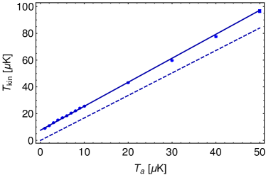
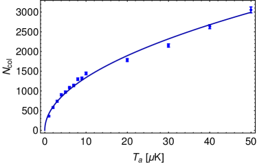
Figure 1: Equilibrium average kinetic energy in units of $T_{\rm{kin}}$ of a single ion colliding with atoms (left) and number of collisions required to equilibrate (right) versus temperature of the atoms. The results were fit with a linear function (solid line, left) or a square root function (solid line, right) respectively. The dashed line corresponds to a hypothetical case without micromotion-induced heating as explained in the text.

The average kinetic energy of the ion (left) in units of $T_{\rm{kin}}$ shows a strictly linear dependence with a slope of 1.79(2) and offset of $7.60(14)\,\mu$K. The dashed line shows the hypothetical case in which each secular mode of the ion equilibrates with the temperature of the atom, according to the approximate prediction of Eq. 7. Its slope reads 1.68 using the trap parameters of the simulation. In particular, the deviation from unity slope is given by the extra energy stored in the micromotion amplitude, which is approximately $\frac{1}{2}k_{\rm{B}}T_{\rm{a}}$ extra per radial direction [43], such that the energy of the atomic bath excites five kinetic degrees of freedom instead of three, explaining the slope of approximately $5/3$. The deviation in slope of the simulated points with respect to the prediction is expected to be caused by the approximations made to obtain the prediction (i.e. $|a_{i}|$ and $q_{i}^{2}\ll 1$, see Sec. 2.1). The offset can be seen as the direct influence of micromotion-induced heating, transferring energy from the trap drive rf field into the secular motion of the ions, mediated by the atoms. The number of collisions required to equilibrate (right) follows a square root function, which is to be expected, since the thermalization rate $\Gamma_{\rm{eq}}=1/N_{\rm{col}}$ should be directly proportional to the fraction of events that lead to thermalization, namely Langevin collisions, divided by the number of total events, $\Gamma_{\rm{eq}}\propto\frac{\Gamma_{\rm{L}}}{\Phi(\vec{v}_{\rm{a}})}$, with $\Gamma_{\rm{L}}$ the Langevin rate and $\Phi(\vec{v}_{\rm{a}})$ the flux into the sphere on which the atoms start as defined in Eq. 19. Thus, $N_{\rm{col}}\propto\Phi(\vec{v}_{\rm{a}})\propto\sqrt{T_{\rm{a}}}$ . From the fit, we obtain a proportionality factor of $412(8)/\sqrt{\mu{\rm{K}}}$

4.2 Influence of radial excess micromotion

In this paragraph, we investigate the influence of radial excess micromotion caused by a stray electric field $\vec{E}_{\rm{rad}}$ on the average kinetic energy of a single ion when immersed in a cold atomic bath of $2\,\mu$K. We scanned $E_{\rm{rad}}$ over a range of 0.0 to 0.6 V/m and determined the ion’s average kinetic equilibrium energy in units of $T_{\rm{kin}}$ and the typical number of collisions required to equilibrate $N_{\rm{col}}$ according to Eq. 25 by averaging over at least 300 individual runs for each point. We additionally checked the influence of the radial direction of $E_{\rm{rad}}$. The results are shown in Fig. 2.

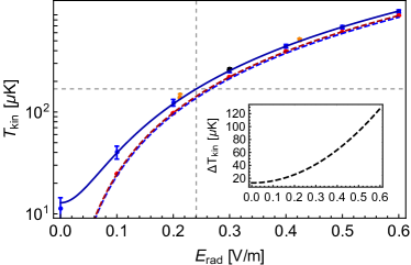
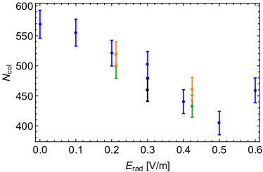
Figure 2: Equilibrium temperature of a single ion colliding with atoms at $2\,\mu$K (left) and number of collisions required to equilibrate (right) versus radial electric offset field. The results (blue points) were fit with a quadratic function (solid blue curve). The red points correspond to the average kinetic energy of an ion initialized at zero secular temperature without an atomic bath, along with a quadratic fit (red dashed curve) and the approximate theoretical amount of micromotion energy (blue dashed curve). The dashed gray lines indicate the $s$-wave temperature limit for $T_{\rm{a}}\rightarrow 0$. The inset shows the difference between the solid and dashed blue curve, resembling the micromotion induced heating. Other colors are explained in the text.

The temperatures (blue) were calculated using a radial electric field in $x$-direction only. The results were fit with a quadratic function (solid blue line),

$$T_{\rm{kin}}=T_{1}+\theta_{E_{\rm{rad}}}E_{\rm{rad}}^{2}\,,$$ (26)

leading to a quadratic rise factor of $\theta_{E_{\rm{rad}}}=2680(15)\,\mu{\rm{K}}\cdot\left(\rm{V/m}\right)^{-2}$. The dashed blue curve represents the approximate theoretical amount of kinetic energy due to the presence of excess micromotion, according to Eq. 10, with a quadratic rise factor of $2360\,\mu{\rm{K}}\cdot\left(\rm{V/m}\right)^{-2}$. Also shown is the average kinetic energy for an ion without an atomic bath present, initialized at zero temperature (red points) along with a quadratic fit (red dashed line). The difference between the solid blue curve and the dashed red curve corresponds approximately to the amount of energy stored in the intrinsic micromotion and the secular motion. The point at $E_{\rm{rad}}=0.3\,$V/m was simulated once with a factor 10 smaller tolerance parameter $p_{\rm{tol}}$ in the propagator to check for numerical errors. The values in orange were taken using a dc field with equal components $E_{\rm{rad},x}=E_{\rm{rad},y}$ in both radial directions, the values in green (behind the orange points) with a dc field with opposite components, $E_{\rm{rad},x}=-E_{\rm{rad},y}$, to check the influence of the direction of $E_{\rm{rad}}$, showing no deviation from the fitted curve. The number of collisions required to equilibrate (right) seems to slightly decrease with increasing field amplitude.

4.3 Influence of axial micromotion

In this paragraph, we investigate the influence of a homogeneous oscillating electric field along the axial direction of the trap on the average kinetic energy of a single ion when immersed in a cold atomic cloud at $2\,\mu$K. We scanned the field amplitude $E_{\rm{ax}}$ from $0-15\,$V/m and determined the ion’s average kinetic equilibrium energy in units of $T_{\rm{kin}}$ and the typical number of collisions required to equilibrate $N_{\rm{col}}$ according to Eq. 25 by taking the average over at least 300 idividual runs for each point. The results are shown in Fig. 3.

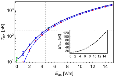
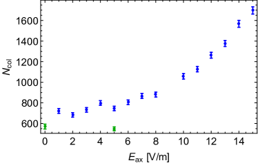
Figure 3: Equilibrium temperature of a single ion colliding with atoms at $2\,\mu$K (left) and number of collisions required to equilibrate (right) versus axial rf-field amplitude. The temperatures (blue) were fit with a quadratic function (solid blue curve). The red points correspond to an ion initialized at zero secular temperature without the presence of an atomic bath, in agreement with the approximate theoretical amount of micromotion energy (dashed blue curve). The dashed gray lines indicate the $s$-wave temperature limit. The inset shows the difference between the solid and dashed blue curve, resembling the micromotion induced heating. Colors are explained in the text.

The temperatures (blue) were fit with a quadratic function (solid blue curve),

$$T_{\rm{kin}}=T_{1}+\theta_{E_{\rm{ax}}}E_{\rm{ax}}^{2}\,,$$ (27)

leading to a quadratic rise factor of $\theta_{E_{\rm{ax}}}=7.44(3)\,\mu{\rm{K}}\cdot\left(\rm{V/m}\right)^{-2}$. The dashed blue curve represents the approximate theoretical amount of kinetic energy due to the axial oscillating electric field, according to Eq. 13, with a quadratic dependence of $6.92\,\mu{\rm{K}}\cdot\left({\rm{V/m}}\right)^{-2}$, in agreement with the points in red, showing the average kinetic energy of a crystal at zero secular energy without atoms present.

Due to the large axial oscillation amplitudes at high values of $E_{\rm{ax}}$, a fixed starting sphere causes the atoms to occasionally launch very close to the ion, thus introducing unrealistic jumps in the potential energy that can lead to unstable behavior. Therefore, the blue points were not obtained using a starting sphere with fixed origin at the ion’s equilibrium position, but a comoving sphere around the ion’s immediate position. As a consequence, there are events where the ion is moving away from the introduced atom such that the atom is immediately registered as having escaped, leading to an increased number of required collisions, (Fig. 3 right, blue points) as compared to the non-comoving case (green points). This effect seems to increase with field amplitude. A comoving starting sphere means that especially very slow atoms that would usually cause a Langevin collision are overseen. Therefore, the average contribution of the atom to the collision energy increases. Since the ion temperature in this regime is dominated by the micromotion energy anyways, this effect can be ignored.

4.4 Influence of quadrature micromotion

The effect of phase micromotion on the equilibrium average kinetic energy of a single ion in an atomic gas of $2\,\mu$K is investigated. We scanned the phase difference $\delta\phi_{\rm{rf}}$ from 0-0.65 mrad, corresponding to the expected experimental upper limit from the linewidth broadening measurement as discussed in 3. We determined the resulting equilibrium average kinetic energy in units of $T_{\rm{kin}}$ as well as $N_{\rm{col}}$ according to Eq. 25 by averaging over at least 300 individual runs per point. The results are shown in Fig. 4.

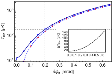
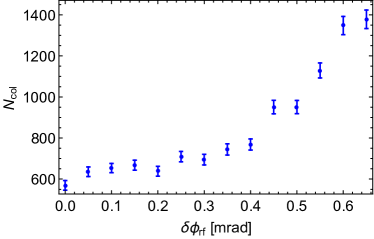
Figure 4: Equilibrium temperature of a single ion colliding with atoms at $2\,\mu$K (left) and number of collisions required to equilibrate (right) versus phase mismatch of the two radial rf-components of the potential. The temperatures (blue) were fit with a quadratic function (solid blue curve). The red points correspond to an ion initialized at zero secular temperature without the presence of an atomic bath, in agreement with the approximate theoretical amount of micromotion energy (dashed blue curve). The dashed gray lines indicate the $s$-wave temperature limit. The inset shows the difference between the solid and dashed blue curve, resembling the micromotion induced heating.

The temperatures (blue) were fit with a quadratic function (solid blue line),

$$T_{\rm{kin}}=T_{1}+\theta_{\delta\phi_{\rm{rf}}}\delta\phi_{\rm{rf}}^{2}\,,$$ (28)

leading to a quadratic rise factor of $\theta_{\delta\phi_{\rm{rf}}}=3980(15)\,\mu{\rm{K}}\cdot{\rm{mrad}}^{-2}$. Also shown is the approximate theoretical amount of kinetic energy stored in the phase micromotion (dashed blue), according to Eq. 16, with a quadratic increase of $3651.2\,\mu{\rm{K}}\cdot{\rm{mrad}}^{-2}$ for the parameters used in the simulation. As in the case for axial micromotion, the red points show the average kinetic energy of an ion without an atomic bath present, in agreement with the dashed blue line. All points of the plot were simulated using a comoving start and escape sphere for the atoms to prevent numerical instabilities, thus leading to an increasing number of collisions required to equilibrate (right).

5 Ion crystals

In this section, we briefly introduce the theoretical and numerical framework to describe the normal modes of oscillations in an ion crystal. We present and test a numerical method to extract the energy stored in the secular motion of each individual mode.

By treating the mutual Coulomb interaction of the ions as well as the trapping itself in harmonic approximation, the ion crystal can be described as a system of coupled harmonic oscillators. This system can be decomposed into normal mode coordinates and frequencies. This procedure is described in detail in e.g. [52] for a linear ion crystal. For a given set of secular trap frequencies and number of ions, the equation of motion reads

$$m_{\rm{ion}}\ddot{\vec{r}}_{n}=\vec{F}_{n}=-m_{\rm{ion}}\hat{\omega}^{2}\vec{r}_{n}+\frac{e^{2}}{4\pi\epsilon_{0}}\sum_{m\neq n}\frac{\vec{r}_{n}-\vec{r}_{m}}{\left\|\vec{r}_{n}-\vec{r}_{m}\right\|^{3}}\,,$$ (29)

where the first term describes the three-dimensional trapping of each ion with the trap frequency matrix $\hat{\omega}={\rm{diag}}\left(\omega_{x},\omega_{y},\omega_{z}\right)$ and the second term is the mutual Coulomb interaction of the $N$-ion system. To obtain the transformation matrix to transform the system into normal mode coordinates, one first has to find the equilibrium positions $\vec{r}_{n}^{\,(0)}$ of the ions within the trap, defined as $\vec{F}_{n}(\vec{r}_{n}^{\,(0)})=0\,$. We do this in a two-step process: First, we numerically simulate the cooling of an $N$-ion system in our trap until it crystallizes by introducing an additional velocity-dependent force in the equation of motion,

$$m_{\rm{ion}}\ddot{\vec{r}}_{n}=\vec{F}_{n}-\kappa\dot{\vec{r}}_{n}\,,\quad\kappa>0\,.$$ (30)

As a second step, we use the numerically obtained equilibrium positions as a guess for numerically finding the positions where the force on the ions disappears. This procedure was found to be more stable than immediate minimization of force on the ions, especially for higher dimensional crystals.

Treating the coordinates of the ions as small deviations from their equilibrium positions, $\vec{r}_{n}(t)\approx\vec{r}_{n}^{\,(0)}+\vec{\rho}_{n}(t)$, the potential energy of the system can be expanded to second order in $\vec{\rho}_{n}$ to

$$U =\sum_{n=0}^{N_{\rm{ions}}}\frac{1}{2}m_{\rm{ion}}\bar{\omega}^{2}\vec{r}_{n}^{\,2}+\frac{1}{2}\frac{e^{2}}{4\pi\epsilon_{0}}\sum_{n\neq m}\frac{1}{\left\|\vec{r}_{n}-\vec{r}_{m}\right\|}$$ (31)

$$\approx\frac{1}{2}m_{\rm{ion}}\omega_{z}^{2}\sum_{i,j=1}^{3}\sum_{m,n=1}^{N_{\rm{ions}}}A_{3(m-1)+i,3(n-1)+j}\rho_{m,i}\rho_{n,j}\,.$$ (32)

With the $3N_{\rm{ions}}\times 3N_{\rm{ions}}$ Hessian matrix $A_{3(m-1)+i,3(n-1)+j}=\left.\frac{\partial^{2}U}{\partial r_{m,i}\partial r_{n,j}}\right|_{0}$, where $r_{m,i}$ is the coordinate of ion $m$ in the $i$-th direction and the 0 denotes its evaluation at equilibrium positions. For clarity we rename the indices of A to $u=3(m-1)+i$, $v=3(n-1)+j$, $u,v\in\{1,\dots,3N_{\rm{ions}}\}$. Diagonalization of the symmetric Hessian matrix leads to the diagonal form $D_{u,v}$ that can be obtained from the transformation $D=S^{T}AS$, where S is the matrix of eigenvectors of $A$. The $3N_{\rm{ions}}$ eigenmode frequencies $f_{q_{u}}$ are then given by $2\pi f_{q_{u}}=\omega_{q_{u}}=\omega_{z}\sqrt{D_{u,u}}$ and the potential energy in secular approximation reads

$$U_{\rm{sec}}=\frac{1}{2}m_{\rm{ion}}\sum_{u=1}^{3N_{\rm{ions}}}\omega_{q_{u}}^{2}q_{u}^{2}\,,$$ (33)

with $q_{u}=\sum_{n=1}^{N_{\rm{ions}}}\sum_{j=1}^{3}S_{u,3(n-1)+j}\rho_{n,j}$ the normal mode coordinates.

Once transformed to these coordinates, the trajectories stored in each kinetic energy determination are Fourier transformed numerically using a standard Cooley-Tukey fast Fourier transform (FFT) algorithm [53]. The Fourier spectra of the normal coordinates then contain only a peak at the respective mode frequency along with peaks at the micromotion sidebands. To obtain the energy stored in each mode, we compute the average kinetic energy of each normal coordinate $q_{m}$,

$$\bar{E}_{m,{\rm{tot}}}=\frac{1}{2}m_{\rm{ion}}\frac{1}{N_{\rm{fft}}}\sum_{k=1}^{N_{\rm{fft}}}\dot{q}_{m}(t_{k})^{2}\,,$$ (34)

where $m$ is the mode index and $k$ the time index of the Fourier time grid of spacing $\Delta t_{\rm{fft}}$. Since this energy still contains micromotion, we make use of the Fourier relation for time derivatives,

$$(\mathcal{F}\dot{q}_{m})(f)=-i2\pi f\tilde{q}_{m}(f)\,,$$ (35)

where $\tilde{q}_{m}(f)=(\mathcal{F}q_{m})(f)$ is the Fourier transform of the normal coordinate $q_{m}(t)$, and Parseval’s theorem for the discrete Fourier transformation,

$$\sum_{k=1}^{N_{\rm{fft}}}||\dot{q}_{m}(t_{k})||^{2}\Delta t_{\rm{fft}} =\sum_{k=1}^{N_{\rm{fft}}}||-i2\pi f_{k}\tilde{q}_{m}(f_{k})||^{2}\Delta f_{\rm{fft}}$$ (36)

$$=(2\pi)^{2}\Delta f_{\rm{fft}}\sum_{k=1}^{N_{\rm{fft}}}f_{k}^{2}\tilde{q}_{m}(f_{k})\tilde{q}_{m}^{*}(f_{k})\,,$$ (37)

with which we can replace the expectation value of the squared normal mode velocity $\dot{q}_{m}(t)$ and obtain

$$\bar{E}_{m,{\rm{tot}}}=\frac{1}{2}m_{\rm{ion}}(2\pi)^{2}\Delta f_{\rm{fft}}^{2}\sum_{k=1}^{N_{\rm{fft}}}f_{k}^{2}\tilde{q}_{m}(f_{k})\tilde{q}_{m}^{*}(f_{k})=\frac{1}{2}k_{B}T_{m}\,,$$ (38)

using the identity for the Fourier frequency grid spacing $\Delta f_{\rm{fft}}=(N_{\rm{fft}}\Delta t_{\rm{fft}})^{-1}$. To test the validity of this method, the total kinetic energy of all modes

$$\bar{E}_{\rm{tot,fft}}=\sum_{m=1}^{3N_{\rm{ions}}}\bar{E}_{m,{\rm{tot}}}=\frac{3N_{\rm{ions}}}{2}k_{\rm{B}}T_{\rm{fft}}\,,$$ (39)

can be compared with the average kinetic energy defined in Eq. 22, which is presented in section B. Since typically all secular frequencies are separated far from the micromotion frequency, the high frequency parts of the spectrum can be cut off easily by reducing the limit of the sum in Eq. 38 to a value $N_{\rm{c}}=f_{\rm{c}}/\Delta f_{\rm{fft}}$, where $f_{\rm{c}}$ is the desired cut-off frequency. To obtain only the secular energy part for each of the modes $\bar{E}_{m,{\rm{sec}}}$, the cut-off frequency should be chosen centered between the highest normal mode frequency and the lowest micromotion sideband. We define the temperature of each mode by $T_{m,{\rm{sec}}}$ and the total secular temperature as $T_{\rm{sec}}$ as

$$\bar{E}_{\rm{sec}} =\sum_{m=1}^{3N_{\rm{ions}}}\bar{E}_{m,{\rm{sec}}}=\sum_{m=1}^{3N_{\rm{ions}}}\frac{1}{2}k_{\rm{B}}T_{\rm{m,sec}}=\frac{3N_{\rm{ions}}}{2}k_{\rm{B}}T_{\rm{sec}}\,.$$ (40)

The approximate eigenmode frequencies $f_{q_{m}}$ can be found by searching the peak position of the Fourier spectrum for the respective mode within an accuracy of the Fourier frequency grid size $\Delta f_{\rm{fft}}=1/(N_{\rm{fft}}\Delta t_{\rm{fft}})$ leading to a relative error typically on the order of $\frac{1}{2}\Delta f_{\rm{fft}}/f_{q_{m}}$.

A typical spectrum of the Fourier amplitudes for a linear four-ion crystal is shown in Fig. 5. The Fourier spectra of all spatial coordinates (left) show each multiple peaks at the twelve different mode frequencies. The spectrum also contains the micromotion sidebands around the trap drive frequency of $f_{\rm{rf}}=2\,$MHz and a possible cutoff value (gray bar) for the secular energy determination. While some of the peaks at around 130 kHz are too close to be distinguished, the Fourier spectra of the normal mode coordinates (right) show only one peak each, allowing for the numerical frequency and energy determination within each mode. Note that the plots are cut off at the relevant eigenmode frequency scale, not showing the micromotion sidebands around the trap drive frequency $f_{\rm{rf}}=2\,$MHz.

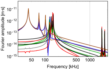
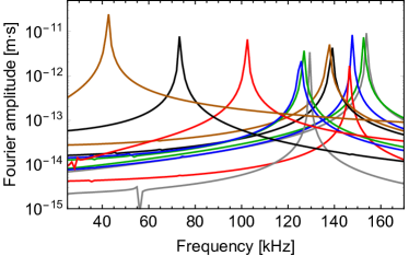
Figure 5: Fourier amplitudes for the twelve spatial coordinates (left) and for the twelve normal coordinates (right) for a simulated linear four-ion crystal at an average kinetic energy of around $5\,\mu$K. Each spatial coordinate shows contributions of multiple frequencies, whereas the normal modes are clearly decoupled and show only a single peak at the respective mode frequency. For the spatial coordinates, the micromotion sidebands around $f_{\rm{rf}}=2$ MHz and the cutoff frequency (gray bar) for the secular energy determination are shown as well. The Fourier spectra were obtained using $N_{\rm{fft}}=16384$ steps of $\Delta t_{\rm{fft}}=50\,$ns.

The twelve normal modes of the four-ion crystal are visualized in Fig. 21 in Appendix B, along with their respective frequencies obtained from the diagonalization of the secular case as presented in this section and the frequency peak positions of the fourier spectra. Typically, these modes are assigned with the names given in the right column [54].

6 Ion crystals in the cold buffer gas

In this section, we investigate the influence of the number of ions as well as that of all types of micromotion in an ion crystal. We further analyze the case where an additional oscillating electric quadrupole field in axial direction is present, leading to a non-vanishing $q_{z}$-parameter, which is typically the case under realistic experimental conditions. In this section, we assume that the entire crystal is immersed in the atomic cloud, and each ion is equally likely to collide with an atom. In particular, we dice the ion at which the atom is introduced before calculating each collision event.

6.1 Influence of the number of ions

First, the influence on the achievable temperature of the crystal $T_{\rm{kin}}$ (see Eq. 22) and typical number of collisions required to equilibrate $N_{\rm{col}}$ as defined in Eq. 25 was investigated. The results for one to six ions trapped using no axial or excess radial micromotion is shown in Fig. 6. For one and two ions at least 300 runs were averaged, whereas due to the computational effort for three to six ions, only 40 runs each were simulated, thus leading to worse statistics and thus larger errors.

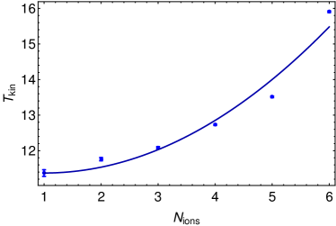
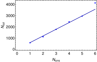
Figure 6: Final temperature $T_{\rm{kin}}$ (left) and the number of collisions required to equilibrate (right) versus number of ions in a linear crystal colliding with atoms at $2\,\mu$K. The kinetic energy shows a weak dependence on number of ions, whereas $N_{\rm{col}}$ is strictly linear.

For the final temperature of the crystal (left) a weak dependence on number of ions can be observed. The results were fit with a heuristic fit function (blue line),

$$T_{\rm{kin}}=T_{1}+\theta_{\rm{i}}\left(N_{\rm{ions}}-1\right)^{2}\,,$$ (41)

leading to $T_{1}=11.4(2)\,\mu$K and a quadratic rise factor of $\theta_{\rm{i}}=0.17(2)\,\mu{\rm{K}}$. The number of collisions required for thermalization (right) is strictly linear in number of ions. The linear fit (solid line) leads to an increase of 626(20) collisions per additional ion. The behavior is to be expected since the number of modes of the crystal that need to be cooled increases linearly as well. While in the simulation only one atom is introduced at a time, in the experiment the density of atoms ideally is the same all along the ion crystal, thus increasing the actual collision rate by the factor $N_{\rm{ions}}$. Consequently, the thermalization time for an $N_{\rm{ions}}$-crystal is expected to be the same as for one ion.

6.2 Influence of excess micromotion

Similar to the single ion case, the effect of radial excess micromotion as well as axial micromotion and quadrature micromotion was investigated. Additionally, the dependence of the secular energy was studied. The obtained results can be found in C. The behavior of the final average kinetic energy versus the scanned micromotion parameter is in perfect agreement with the single ion case.

6.3 Influence of a non-vanishing axial rf-gradient ($q_{z}\neq 0$)

To study the effect of a non-vanishing $q_{z}$, the parameter was scanned from 0 to 0.005. The value in our ion trap is around $q_{z}^{\rm{exp}}=0.0023$ for similar trapping parameters as used in the simulation. The resulting equilibrium Temperatures $T_{\rm{kin}}$ and $T_{\rm{sec}}$ are shown in Fig. 7 (blue). The points were obtained by averaging over at least 30 individual runs for each value of $q_{z}$ and fitting the averages according to Eq. 25.

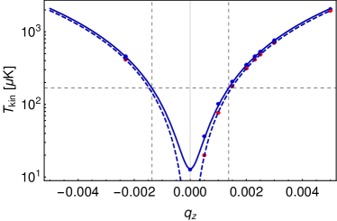
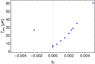
Figure 7: Equilibrium temperature of a linear four-ion crystal colliding with atoms at $2\,\mu$K (left) and secular temperature (right) versus $q_{z}$ parameter. The left points (blue) were fit with a quadratic function and an offset (solid curve). The dashed curve shows the approximate theoretical behavior as explained in the text. The dashed gray lines indicate the $s$-wave temperature limit for $T_{\rm{a}}\rightarrow 0$. The red dots were obtained from a simulation with zero secular energy and no atoms present.

The results for the average kinetic energy (left) were fit using a quadratic function with offset (solid line), $T_{\rm{kin}}(q_{z})=T_{1}+\theta_{q_{z}}q_{z}^{2}$, leading to a quadratic rise factor of $\theta_{q_{z}}=8.29(6)\cdot 10^{7}\,\mu{\rm{K}}$ with offset $T_{\rm{1}}=13.0(6)\,\mu{\rm{K}}$. The approximate theoretical dependence of the average kinetic energy according to Eqs. 9-10 is shown as a dashed line. The quadratic rise of the theoretical curve is given by $\theta_{q_{z}}^{\rm{theo}}=7.80\cdot 10^{7}\,\mu$K. The points in red show the average kinetic energies due to the influence of $q_{z}$ in the non-interacting case where the ions were initialized without secular energy. A quadratic fit of the red points lead to a rise factor of $\theta_{q_{z}}^{(0)}=7.81(1)\cdot 10^{7}\,\mu{\rm{K}}$, in good agreement with the prediction from the approximate solution, which is to be expected as the approximation holds for $q_{z}^{2}\ll 1$. The secular temperature (right) shows an almost linear dependence on $q_{z}$ and resembles the actual influence of the additional micromotion-induced heating due to a non-vanishing $q_{z}$.

6.4 Micromotion-induced heating on the individual modes

In this section, we analyze the effect of each type of micromotion on the individual modes of a four-ion crystal. The secular temperature of each mode was obtained as described in section 5 from the simulations of the linear four-ion crystal in section 6.2 and 6.3. The resulting temperatures for the twelve individual modes as presented in Fig. 21 are shown in Fig. 8 for radial excess micromotion (left top) axial micromotion (right top) and quadrature micromotion (left bottom).

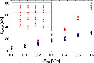
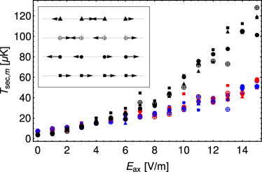
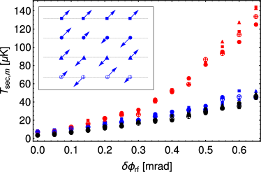
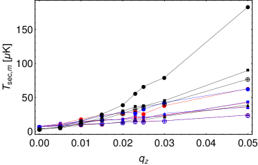
Figure 8: Individual secular temperatures $T_{\rm{sec},m}$ of each normal mode of a linear four-ion crystal colliding with atoms at $T_{\rm{a}}=2\,\mu$K in the case of a radial dc electric field $E_{\rm{rad}}$ in $x$-direction (left top), a homogeneous axial oscillating field (right) with amplitude $E_{\rm{ax}}$ (right top) or in the presence of a rf phase shift $\delta\phi_{\rm{rf}}$ between the rf electrodes (left bottom). The results depicted in red and blue were obtained from the four modes oscillating in $x$- or $y$-direction respectively, whereas the results in black were obtained from the four axial modes. The plot on the down right shows the behavior of the twelve secular mode temperatures for a non-vanishing $q_{z}$ parameter. The insets illustrate the respective modes, in which the arrows indicate the direction and relative amplitude of motion.

In each of the three cases the radial modes equilibrate to a slightly higher temperature than the axial modes, when the scanned excess micromotion parameter is low. For high values the temperature of the modes with excess micromotion dominate, which is the $x$-direction (red) for both radial and quadrature micromotion and the $z$-direction (black) in the case of axial micromotion. A further sub-separation of the radial and axial modes is not resolved.

Interestingly, for a non-vanishing axial gradient, expressed by $q_{z}$, the situation is quite different, as it is shown in Fig. 8. In this case, the modes separate for high $q_{z}$ into different groups, starting with the $x$ and $y$ zigzag modes (red and blue crossed circles) at the lowest temperature for $q_{z}=0.05$. The next group is formed by the $x$ and $y$ center-of-mass modes (red and blue squares) along with the drum modes (red and blue triangles) and the $z$ anti-stretch mode (black triangles). Approximately located at mode average temperature the two tilt modes (red and blue circles) are found. At higher temperature, the three remaining axial modes Egyptian (black crossed circles), center-of-mass (black squares) and stretch (black circles) are located. This behavior is mainly reasoned by the participation of the outer ions to these modes, since these can exchange the largest amount of energy during a collision due to their large micromotion amplitudes. While the contribution of the outer ion’s motion to the zigzag modes is lowest and the mode is moving perpendicular to the micromotion direction, the radial center-of-mass and drum modes show larger and equal coupling as indicated by the arrow length in the mode visualization insets and in table 21. The anti-stretch mode shows less coupling strength for the outer ions but moves in the direction of micromotion, thus enhancing the probability for a high energy exchange within a collision. The strongest radial contribution of the outer ion’s motion is to the two tilt modes, leading to the highest radial mode temperatures. As in the case of an homogeneous oscillating axial field, the highest temperatures are found within axial modes, dominated by the one with the largest contribution of the outer ion’s motion, the stretch mode.

7 Two-dimensional ion crystals

By adjusting the axial and radial trapping fields, it is possible to change the shape and dimensionality to form two dimensional ion crystals [55, 56, 57, 58]. Even with perfect micromotion compensation, there are always ions within any nonlinear crystal that have their quasi-equilibrium position outside the radiofrequency node axis, thus experiencing a non-vanishing oscillating electric field, leading to additional, unavoidable micromotion. Therefore, immersing the complete ion crystal in a cloud of ultracold atoms will always lead to micromotion-induced heating of the normal modes. To avoid this effect, one can utilize the large spacing between the ions, enabling the experimental possibility to overlap a dense and small atomic cloud only with a single ion sitting at the axial radiofrequency node within a larger ion crystal.

To simulate a stable 7-ion hexagonal ion crystal, we change the trap parameters to $f_{z}=95.459\,$kHz, $q_{x}=q_{y}=0.261$, and $\alpha_{x}=1.0$, $\alpha_{y}=-2.0$ to achieve $f_{x}=211.002\,$kHz and $f_{y}=127.229\,$kHz as radial secular trap frequencies, all within experimental reach with the ion trap used in our experiment. Due to the stronger confinement in the $x$-direction, the crystal forms in the $y-z$ plane. Its geometry along with its approximate (secular) mode structure is depicted in Fig. 9. Notably, in contrast to a linear crystal, the mode with the highest frequencies are not center-of-mass modes, but the two planar blink modes, where the ion density oscillates in $y$ and $z$ direction respectively. Also the mode with the lowest frequency is not a center-of-mass mode but the x rotate mode, where all six ions defining the hexagon oscillate in phase clockwise/counterclockwise around the central ion within the crystal plane.

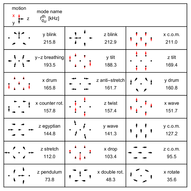
Figure 9: Visualization of the normal mode movement for a trapped planar seven-ion crystal. The arrows indicate the direction and amplitude of the respective mode within the plane (black) and perpendicular to the plane (red). For each mode the respective eigenfrequency $f_{q_{u}}^{\rm{th}}$ obtained from diagonalization of the secular approximation is shown.

To simulate the thermalization of the secular modes, we initialize the ion crystal with negligible secular energy by first switching on a strong velocity-dependent damping force as defined in Eq. 30 that is adiabatically turned to zero. To give the ion crystal an initial secular energy, we add to each ion’s velocity components a velocity sampled from a Maxwell-Boltzmann distribution at a given temperature before the first collision occurs. We only let the central ion collide with atoms at $T_{\rm{a}}=2\,\mu$K. We obtain the secular temperatures for each mode as in the case for the linear ion crystal by integrating over the Fourier spectra of the normal mode coordinates. Due to the orders of magnitude larger micromotion sidebands around the trap frequency of $2\,$MHz, it is necessary to increase the frequency resolution by a factor of four and only take a narrow range around the respective peaks for the integrals into account. Otherwise, the integrals suffer from a non-neglegible micromotion floor of the Fourier spectra even around the secular frequencies that can only be suppressed by further increasing the Fourier resolution towards unfeasible computational effort. To compensate for the already large increase in computation time due to the large micromotion amplitudes and increased number of particles compared to the four-ion linear crystal, the atom start sphere size was chosen to be fixed and only $r_{0}=0.3\,\mu$m around the central ion, thus increasing the likelihood of Langevin collisions but also cutting down the propagation times during a collision. The results for all 21 modes of a planar seven-ion crystal initialized at $25\,\mu$K are shown in Fig. 10. The values were averaged over 120 individual runs.

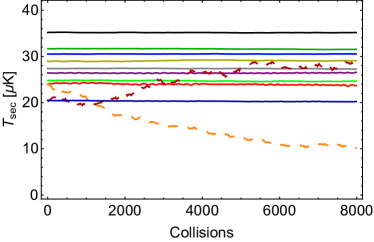
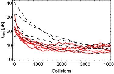
Figure 10: Thermalization of the secular modes of a hexagonal planar seven-ion crystal initialized at a secular temperature of $25\,\mu$K when only the central ion is colliding with atoms at $2\,\mu$K. The modes without motional components of the central ion (left) show almost no dynamic, whereas all other modes (right) thermalize to temperatures below $20\,\mu$K.

The thermalization of the modes can be classified into three different groups.

• The modes where the central ion’s motion is not participating at all do not show significant cooling dynamics (left), besides the y drum (orange dashed) and y wave (dark red dashed) mode, showing a relatively slow cooling and heating, possibly due to enhanced nonlinear Coulomb interactions between the ions in these two modes.

• The modes where the central ion participates rather weakly (right, black dashed), as indicated by the length of the vectors in Fig. 10, show a slow cooling dynamic over the observed number of collisions.

• The modes where the central ion participates most (right, solid red), x/z blink, x drop, z pendulum and x double rotation, thermalize the fastest.

The different initial temperatures of each mode are caused by the different coupling strength and number of modes each ion is involved in and could in principle be corrected for, but this is not necessary for the qualitative analysis of the behavior. Remarkably, the achieved minimum temperatures of the modes that thermalize are all found to be between $5\,\mu$K, and $15\,\mu$K, comparable to the secular temperatures achieved using the linear four-ion crystal at perfect micromotion compensation, although the average kinetic energy of the planar crystal $T_{\rm{kin}}=700\,$mK is five orders of magnitude larger due to the large micromotion amplitudes of the outer ions.

8 Conclusions

In this article we have presented numerical simulations of classical Yb⁺-Li collisions for ions trapped in a Paul trap. We presented and tested a numerical framework to simulate and analyze the collisions using parameters that can be achieved in our experiment, including all types of micromotion that are observable in real ion traps. We analyzed the effect of the micromotion on the achievable average kinetic energy of a single ion. For an ion in an ideal Paul trap and in the limit where $T_{\rm{a}}\rightarrow 0$, this energy is found to be at $T_{\rm{kin}}=7.60(14)\,\mu$K. Owing to the large mass ratio, this leads to a collision energy of $T_{\rm{col}}=$ 0.4 $\mu$K which lies well below the $s$-wave temperature limit. In this situation, the ion is cooled close to its ground state of motion with $\bar{n}=1.2$ motional quanta remaining in the secular motion on average.

For the limits for all types of excess micromotion found in our experiment, the determined collision energies are a factor of 2-11 higher than the $s$-wave temperature limit, as it is shown in Table 2. This indicates that better micromotion detection and compensation is required there. In particular, using a narrow linewidth laser would allow to put better limits on the axial and quadrature micromotion amplitudes. Another option may be to use the atoms themselves for accurate micromotion detection as described in Ref. [13].

The limits for each experimental parameter that lead to $s$-wave collisions energies are also given in Table 2. Although all lie beyond the limits of our current setup, they are not excessive, as e.g. Härter et al. [13] report a field of $E_{\rm{rad}}\leq 0.02\,$V/m and $E_{\rm{ax}}\leq 0.06\,$V/m in a similar system. For the quadrature micromotion, we expect the given experimental limit of $\delta\phi_{\rm{rf}}=0.65\,$mrad to be overestimated by at least an order of magnitude due to the limitations of our detection techniques, as we show in section 3. The rf phase shift mainly results from unequal length of the connectors, which is approximately less than $\Delta x_{\rm{rf}}\approx 0.5\,$mm. Thus, we expect a phase mismatch on the order of $\delta\phi_{\rm{rf}}\leq\frac{\delta x_{\rm{rf}}}{v_{\rm{rf}}\Omega_{\rm{rf}}}\approx 0.04\,$mrad for an assumed signal propagation velocity of $v_{\rm{rf}}\approx c_{\rm{light}}/2$ half the speed of light. Similarly, we expect that the true axial micromotion amplitude lies significantly below the experimental limit stated. We conclude that Yb⁺/Li may reach the quantum regime with state-of-the-art micromotion compensation. We do note however that our present analysis is based on classical theory. For excellent micromotion compensation, a quantum description such as the one developed in [20] should be generalized to include excess mircomotion and used to predict thermalization in the ultracold regime.

We found that a buffer-gas cooled linear ion crystal behaves similar as a single ion and the presence of more than three modes of ion motion does not significantly influence the achievable collision energies and thermalization rates. A non-vanishing axial gradient expressed as a $q_{z}$-parameter leads to a collision energy of $T_{\rm{col}}=26.3\,\mu$K for a four-ion crystal and the experimental value of $q_{z}^{\rm{exp}}=0.0023$. Also shown in the table are the mean secular energies of the single ion and four ion case along with the mean thermal occupation numbers for the mode with the lowest frequency (center-of-mass).

Within all simulations, we do not observe runaway heating, as expected, since the mass of the ion is much larger than the mass of the atom. In the simulations it takes around $N_{\rm{col}}\approx 550-600$ collisions for a single ion to equilibrate within an atomic cloud with a density of $\rho_{\rm{a}}=\frac{1}{4/3\pi r_{0}^{3}}\approx 1.1\cdot 10^{18}\,{\rm{m}}^{-3}$ (i.e. one atom within the interaction sphere at a time). Within a simulation run using a non-comoving sphere we observe an average flux $\Phi_{\rm{a}}$ of 10000 collisions within 120 ms propagation time, which translates into

$$\Gamma_{\rm L}t_{\rm{col}}=2\pi\rho_{\rm{a}}\sqrt{\frac{C_{4}}{\mu}}\frac{N_{\rm{col}}}{\Phi_{\rm{a}}}\approx 35-38$$ (42)

Langevin collisions that are required for reaching the equilibrium temperature. Luckily, the chance for an inelastic collision happening during the interaction time, leading to charge transfer or molecule formation is less than 0.76 % as we recently measured [49]. The cooling rate for a linear ion crystal is comparable to the single ion case, under the assumption of a homogeneous atomic density all along the ion crystal. Interestingly, the secular modes of a linear ion crystal equilibrate to slightly higher temperatures than average when moving in a micromotion direction.

We have shown that collisional cooling of a planar seven-ion crystal by a localized atomic cloud interacting with only the central ion should be possible. The technique enables cooling of all the ten modes where the colliding ion participates in. The achieved temperatures of these modes are all below $12\,\mu$K, corresponding to mode occupation numbers of $\bar{n}_{m}=\frac{k_{\rm{B}}T_{m,{\rm{sec}}}}{\hbar\omega_{m}}=2-11$ phonons. Shuttling the ion crystal to overlap one of the outer ions with a small atomic cloud at the position of optimal micromotion compensation should in principle increase the number of cooled modes up to 18 out of the 21 total modes. Such localized micro-clouds could be implemented by using a dimple trap as it is described in Ref. [59]. There, the atomic cloud is trapped by a strongly focused laser beam with a waist of $\leq 1.8\,\mu$m, thus trapped in a volume much smaller than the interionic distance, e.g. 14.6 $\mu$m for the ion crystal investigated in this article.

Our results show that with modest improvements in micromotion compensation and detection, reaching the quantum regime of atom-ion collisions can be achieved in our experiment, enabling buffer-gas cooling of the trapped ion quantum platform close to the motional ground state and the observation of atom-ion Feshbach resonances.

	Param.	Value	$T_{\rm{kin}}[\mu{\rm{K}}]$	$T_{\rm{col}}[\mu{\rm{K}}]$	$T_{\rm{sec}}[\mu{\rm{K}}]$	$\bar{n}_{\rm{min}}$	$\bar{n}_{\rm{max}}$
single ion	$E_{\rm{rad}}$	0.3 V/m	257(2)	16(3)	20.9(2)	2.6(1)	8.1(1)
	$E_{\rm{ax}}$	15 V/m	1686(8)	89(4)	86.5(5)	7.0(1)	76.5(1)
	$\delta\phi_{\rm{rf}}$	0.65 mrad	1694(7)	89(4)	75.7(7)	6.4(1)	21.7(1)
four ions	$E_{\rm{rad}}$	0.3 V/m	247(2)	16(3)	20.9(2)	2.5(1)	8.0(1)
	$E_{\rm{ax}}$	15 V/m	1685(7)	89(4)	86.5(5)	7.3(1)	57.7(1)
	$\delta\phi_{\rm{rf}}$	0.65 mrad	1706(6)	90(4)	75.7(7)	6.3(1)	22.0(2)
	$q_{z}$	0.0023	452(4)	26(4)	26.9(1)	2.5(1)	18.0(1)
desired	$E_{\rm{rad}}$	$<$ 0.24 V/m	168.4	8.6	-	-	-
	$E_{\rm{ax}}$	$<$ 4.58 V/m	168.4	8.6	-	-	-
	$\delta\phi_{\rm{rf}}$	$<$ 0.20 mrad	168.4	8.6	-	-	-
	$q_{z}$	$<$ 0.0014	168.4	8.6	-	-	-

Table 2: Simulation results for the different types of micromotion for the single and four-ion case. The collision energies $k_{\rm{B}}T_{\rm{col}}$ are all well above the $s$-wave energy of $E_{s}=k_{\rm{B}}8.6\,\mu$K for the given experimental limits. Also shown are the corresponding minimum and maximum normal mode occupation numbers $\bar{n}_{\rm{min/max}}$ and the desired values to reach collision energies below $E_{s}$ for each micromotion case.

Appendix A Reality checks of the simulation

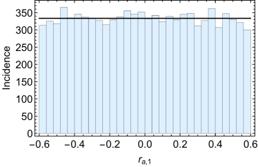
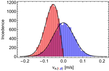
Figure 11: Spatial (left) and velocity (right) distributions of atoms picked on a sphere with radius $0.6\,\mu$m and a temperature of $2\,\mu$K along with the expected probability densities (black).

In this section, we check the accuracy of the simulation algorithm in detail using realistic trapping fields that can be achieved in our experiment. A summary of the parameters used in the simulations unless noted otherwise can be found in table 1.

The functionality of the random number generation was checked by analysis of the distributions of initial atom coordinates for 10000 events sampled at $T_{\rm{a}}=2\,\mu$K on a sphere of $r_{\rm{0}}=0.6\,\mu$m. By definition, the spatial coordinates automatically lie on the sphere. It is therefore sufficient to check that each coordinate is uniformly distributed in the interval $[-r_{0},r_{0}]$. For the velocities, the distributions of Eq. 21 must be obtained. As an example, distributions for $r_{a,1}$, $v_{{\rm{a}},r}$ and $v_{{\rm{a}},\phi}$ are shown in Fig. 11.

Having a method for the energy determination at hand, it is of importance to check the negligible influence of the start- and escape sphere sizes for the atoms. If the sphere radii are picked at the same order as the range of the atom-ion interaction, the immediate change in potential energy after the insertion and extraction of an atom leads to unrealistic kicks in the force on the ion. To check the influence of the sphere radii on the ion temperature, the inner sphere radius $r_{0}$ was scanned between 0.2 and 1.8 $\mu$m. The thermalization of a single trapped ion initially at rest with a thermal cloud of atoms at $2\,\mu$K was simulated. The outer sphere radius $r_{1}$ was chosen to be 0.5 % bigger than $r_{0}$. An example for a thermalization curve (blue points) is shown in Fig. 12 (left). The curve was obtained by averaging over 656 individual runs and fitted with an exponential (see Eq. 25) (black line) leading to an equilibrium temperature of $T_{\rm{kin}}=11.4(1)\,\mu$K on the characteristic time scale of $N_{\rm{col}}=607(2)$ collisions, using $T_{0}=0$ as the initial ion’s temperature. The ion’s energy distribution after thermalization is shown in Fig. 12 (right). The blue points were obtained from all ion energies of the 656 runs between collision 5000 and 10000 and fitted with a thermal distribution (red, dashed) leading to a temperature of $9.4(2)\,\mu$K and a thermal distribution with fixed temperature (purple) obtained from the exponential fit (left). The ion’s energies deviates quite a bit from the thermal distributions, showing a longer tail towards high energies, which is a well known behavior [36, 38, 16, 40], caused by the additional kinetic energy due to the micromotion of the ion.

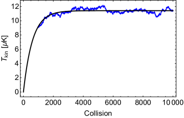
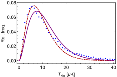
Figure 12: Average kinetic energy of an ion colliding with atoms at $2\,\mu$K averaged over 656 runs to obtain the ion’s temperature (left) from an exponential fit (black) and distribution of the ion’s energies in units of $T_{\rm{kin}}$ as defined in Eq. 22 after thermalization (right) along with a fitted thermal distribution (red, dashed) and a distribution where the temperature was fixed to the value obtained from the exponential fit (purple).

The final temperatures and characteristic number of collisions $N_{\rm{col}}$ required for equilibration for the different starting radii are shown in Fig. 13 and were obtained using the exponential fit model given by Eq. 25. For each point, at least 300 runs were averaged.

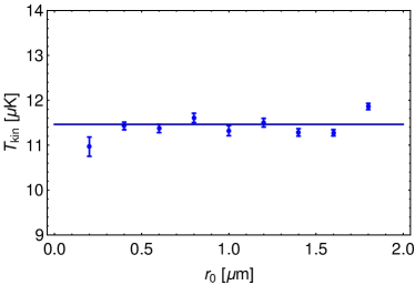
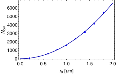
Figure 13: Equilibrium temperature $T_{\rm{kin}}$ as defined in Eq. 22 (left) and characteristic number of collisions $N_{\rm{col}}$ (right) for an ion colliding with atoms at $2\,\mu$K versus the starting distance $r_{0}$ between atom and ion. While the equilibrium temperature does not depend on $r_{0}$ in the scanned regime, the characteristic number of collisions increases quadratically. The lines show a constant (left) and quadratic fit (right).

The equilibrium temperature $T_{\rm{kin}}$ of the ion shows no dependence on the starting sphere size $r_{0}$, whereas $N_{\rm{col}}$ shows a quadratic behavior over the scanned range. This behavior can be qualitatively explained by the nature of Langevin collisions. For a given collision energy $E_{\rm{col}}$, every atom with an impact parameter smaller than $b_{c}=(2C_{4}/E_{\rm{col}})^{1/4}$ undergoes a Langevin collision and can therefore cause a large energy and momentum transfer that contributes to the thermalization process. The fraction of atoms that undergo a Langevin collision $P_{\rm{L}}$ and therefore fly into the solid angle element defined by $b_{c}$ is then given by $P_{\rm{L}}=(1-\cos\left(b_{c}/r_{0}\right))\approx 1/2(b_{c}/r_{0})^{2}$. For an increasing $r_{0}$ this automatically demands for a quadratic increase in the required number of total collisions to equilibrate. Unless noted otherwise, $r_{0}=0.6\,\mu$m is used in all further simulations as a trade-off between simulation time and realistic atomic densities (see e.g. [60]). Demanding only one atom at a time inside the sphere around one of the ions results in a density of $\rho_{\rm{a}}=\frac{1}{4/3\pi r_{0}^{3}N_{\rm{ions}}}<1.1\cdot 10^{18}\,{\rm{m}}^{-3}$.

To realistically model the atom-ion interaction, one needs to check as well that the temperature of the ion does not strongly depend on the choice of the hard-core radius parameter $C_{6}$ as introduced in Eq. 17. In reality, a repulsive barrier is expected to be at a distance, where the electronic wavefunctions of the atom and ion begin to significantly overlap, typically in the range of hundreds of picometers to a few nanometers. The parameter $C_{6}$ was therefore scanned in a range between $5\cdot 10^{-14}\,{\rm{m}}^{2}$ to $5\cdot 10^{-21}\,{\rm{m}}^{2}$, effectively varying the position of the classical turning point $r_{\rm{hc}}=\sqrt{2C_{6}}$ between $0.1\,$nm and $316\,$nm. The results for both final ion temperature $T_{\rm{kin}}$ and collisions required for equilibration $N_{\rm{col}}$ are shown in Fig. 14. The points were obtained by averaging the ion’s average kinetic energy over at least 300 runs and fitting it according to Eq. 25.

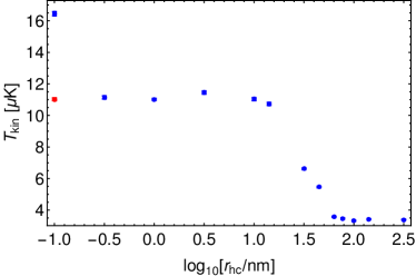
Figure 14: Equilibrium temperature $T_{\rm{kin}}$ as defined in Eq. 22 (left) and characteristic number of collisions $N_{\rm{col}}$ (right) for an ion colliding with atoms at $2\,\mu$K versus the repulsive barrier radius $r_{\rm{hc}}$. The red points were obtained using a higher numerical precision as explained in the text.

For a broad range of barrier radii the final temperature of the ion remains at the same level. For values bigger than $r_{\rm{hc}}=10\,$nm the potential is more and more dominated by the repulsive term proportional to $C_{6}$, preventing Langevin collisions and therefore the ion from micromotion-induced heating as we describe it in our work Ref. [41], where a repulsive barrier is utilized to prevent exactly this heating mechanism. For the smallest value of $r_{\rm{hc}}=0.1\,$nm, the ion temperature seems to be a factor of 1.5 higher than in the regime between 0.3 to 10 nm, which can be explained by numerical errors due to the increasing steepness of the hard core barrier for low values of $r_{\rm{hc}}$ leading to large changes in acceleration in a hard core collision. Therefore, this point was simulated again with a five times smaller tolerance in the adaptive step-size Runge-Kutta propagator, leading to the red points, in agreement with the values for larger $r_{\rm{hc}}$. The number of collisions required for thermalization $N_{\rm{col}}$ seems to first slightly decrease for higher values of $r_{\rm{hc}}$ but shows a dramatic increase by around a factor of two at $r_{\rm{hc}}=77\,$nm. Note that at this point the potential energy minimum caused by the attractive $C_{4}$-term of the potential becomes comparable to the collision energy, dominated by the atom temperature of $2\,\mu$K. Therefore, the intermediately released kinetic energy during a Langevin collision becomes negligible. For even higher values of $r_{\rm{hc}}$ the thermalization process speeds up again due to the quadratically increasing geometric cross section for repulsive collisions. For all further simulations, $r_{\rm{hc}}=1\,$nm is used, which is around three times larger than the classical turning point of the Li-Yb⁺ system [49, 29] but still produces similar results with less numerical effort due to the weaker forces involved.

During propagation, the Runge-Kutta propagator adjusts the size of the time steps in order to stay below a given relative accuracy parameter $p_{\rm{tol}}$. It therefore propagates the system once by a full time step and once by two half time steps and compares the relative difference in propagated coordinates between both methods. If the maximum relative difference between one of the coordinates (including velocity) is bigger than the desired tolerance, the propagation step is repeated using an adjusted time step. To ensure a sufficiently small tolerance $p_{\rm{tol}}$, further tests were performed. Firstly, the allowed tolerance was scanned from $p_{\rm{tol}}=10^{-5}$ to $10^{-15}$ as a parameter for the propagation of a single ion starting at a randomly chosen kinetic energy sampled from a thermal Distribution at $T_{\rm{kin}}=13\,\mu$K, leading to $E_{\rm{kin}}/k_{\rm{B}}=20.5\,\mu$K in the presented case. The trajectories including the velocities for the individual runs were stored to compute the relative deviation in kinetic energy for each tolerance with the one from the smallest value, $p_{\rm{tol}}=10^{-15}$ ,

$$\delta E_{\rm{kin}}(p_{\rm{tol}})=\left|\frac{E_{\rm{kin}}(p_{\rm{tol}})-E_{\rm{kin}}(10^{-15})}{E_{\rm{kin}}(10^{-15})}\right|\,.$$ (43)

Because collisions with atoms can cause a dramatically different change in trajectory for each tolerance, no atoms were introduced in this test. The ions were propagated for $120\,$ms, a timescale that typically corresponds to 10000 collisions in the simulation. Due to the large amount of data, the trajectories were stored only during the last millisecond of propagation. The resulting relative deviations $\delta E_{\rm{kin}}(p_{\rm{tol}})$ are shown in Fig. 15 (left).

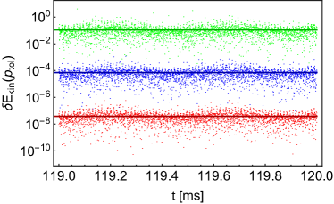
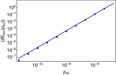
Figure 15: Relative deviations in kinetic energy for a single trapped ion for different values of the adaptive step-size algorithm tolerance $p_{\rm{tol}}$ versus propagation time (left). For clarity only the values for $p_{\rm{tol}}=10^{-6}$ (green), $10^{-10}$ (blue) and $10^{-14}$ is shown in the left plot, along with the time averages (lines). The time averages for the other scanned tolerances are shown on the right, along with an exponential fit.

Due to the adaptive step-size algorithm, it is not possible to have the trajectories for each tolerance stored at the exact same time steps each, therefore the kinetic energy $\delta E_{\rm{kin}}(10^{-15})$ was interpolated using cubic polynomials to match the time grid of the other tolerances, possibly leading to a small amount of interpolation noise. For clarity, only the values for $p_{\rm{tol}}=10^{-6}$ (green), $10^{-10}$ (blue) and $10^{-14}$ (red) are shown along with their time averages (straight lines). In Fig. 15 (right) the time averaged deviations for the other values of $p_{\rm{tol}}$ are shown, approximately following an exponential behavior (solid line) with exponent $n\approx 0.78$ . While for a tolerance of $p_{\rm{tol}}=10^{-6}$ the time averaged relative deviation is $<11\,\%$, $p_{\rm{tol}}=10^{-8}$ delivers acceptable values of $\langle\delta E_{\rm{kin}}(p_{\rm{tol}})\rangle\leq 0.2\,\%$ already.

Similar to the tests for $C_{6}$ and $r_{0}$, also the influence of the tolerance parameter $p_{\rm{tol}}$ on the final ion temperature $T_{\rm{kin}}$ and required collisions $N_{\rm{col}}$ to equilibrate was investigated. The results are shown in Fig. 16. Each point was obtained from taking the average of $\bar{E}_{\rm{kin}}$ over at least 300 individual runs and fitting the curves according to Eq. 25.

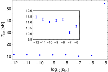
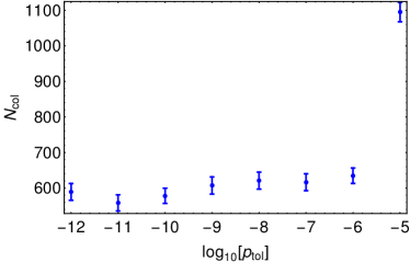
Figure 16: Final ion temperature $T_{\rm{kin}}$ (left) and characteristic number of collisions required to equilibrate $N_{\rm{col}}$ (right) for an ion colliding with atoms at $2\,\mu$K versus tolerance parameter $p_{\rm{tol}}$ used in the adaptive step-size propagator. The inset shows a magnified version of the plot from $p_{\rm{tol}}=10^{-12}$ to $10^{-6}$.

Both observables do not change significantly from $p_{\rm{tol}}=10^{-12}$ to $10^{-6}$, only the point at $p_{\rm{tol}}=10^{-5}$ shows a dramatic increase in both $T_{\rm{kin}}$ and $N_{\rm{col}}$ due to increasing numerical errors. For all further simulations $p_{\rm{tol}}=10^{-10}$ is used (unless noted otherwise) as a trade-off between precision and computational effort.

A final check for both energy conservation of the propagator during collisions as well as physical behavior of the system is to investigate the secular case, where the time-dependent trapping potential of the Paul trap is replaced by a 3D harmonic oscillator potential with the secular trap frequencies of the Paul trap. From a thermodynamic point of view, the ion should then thermalize to the same temperature as the atomic bath and the total energy during each collision should be conserved since no micromotion energy can be transferred to the secular oscillation. The resulting thermalization curve, averaged over 608 individual runs along with a histogram of the energy distribution is shown in Fig. 17.

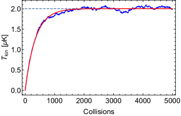
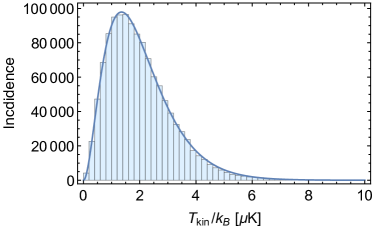
Figure 17: Thermalization curve of a single ion trapped in harmonic oscillator potential colliding with atoms at $2\,\mu$K, using the secular trap frequencies of the employed Paul trap potential (left). The distribution of average kinetic energies according to Eq. 22 in units of $T_{\rm{kin}}$ (right) shows a perfect thermal behavior. The exponential fit (left) as well as the fitted thermal distribution lead to a final temperature of $T_{\rm{ion}}=2\,\mu$K.

The histogram was taken from all points between collision 3000 and 5000 and is in perfect agreement with a thermal distribution (solid line) at $2\,\mu$K, the same temperature as the atomic bath. Also the exponential fit of the thermalization curve (left) leads to the same value, thus indicating a correct physical behavior of the numerical model.

To finally investigate the energy conservation of the collisions, the energy transfer between atom and ion in each collision was investigated by comparing the atom and ion energies before and after a collision, at the points in time $t_{0}$ when an atom is introduced on the sphere with radius $r_{0}$ with the point in time $t_{\rm{1}}$ when that atom escapes the sphere defined by $r_{1}$. The energy transfer on an ion trapped in the harmonic oscillator potential is shown in Fig. 18 (right), taken from one of the 608 individual runs from the simulation used for Fig. 17 (left). The plot shows the ion’s energy transfer $\Delta{E}_{\rm{ion}}={E}_{\rm{ion}}(t_{1})-{E}_{\rm{ion}}(t_{0})$ for each collision and ranges on scales limited by the atom energies. For the atom, a corresponding curve can be obtained. In Fig. 18 (right) the level of energy conservation $\left|\Delta E_{\rm{ion}}+\Delta E_{\rm{atom}}\right|$ is shown.

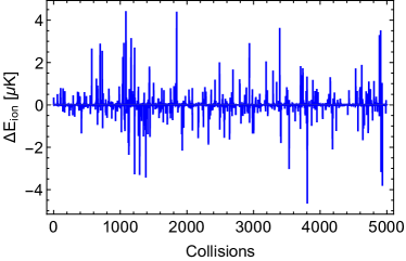
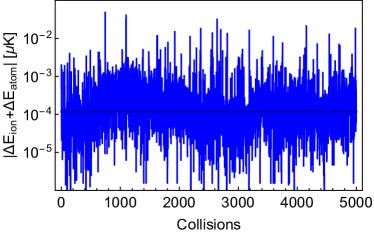
Figure 18: Change in energy of a harmonically trapped ion within each collision with atoms at $2\,\mu$K (left) and total change in energy of the atom-ion system for each collision (right). The solid line shows the averaged energy gain of the system per collision.

The averaged error in total energy in each step is less than 0.12 nK (dark blue line) and therefore negligible on the typical energy scales of the simulations. Note that this error is mainly caused by the sudden but tiny jump in potential energy when the atom is introduced and extracted. With reasonable effort this could be corrected in the energy determination and atom injection scheme, but is only of interest for much higher densities and lower temperatures that may anyways require a quantum mechanical treatment. We therefore conclude that the employed propagator produces physical results with reasonable precision.

Appendix B Reality checks of the Fourier method

In this section, we check the accuracy of the presented Fourier method for determining the average kinetic energy of an ion crystal. Unless stated otherwise, we use a linear chain of four ions at around $100\,\mu$K and let them thermalize by collisions with a cloud of atoms at $2\,\mu$K.

To test the Fourier analysis method for obtaining the temperature of an ion crystal, we compare the temperature $T_{\rm{fft}}$ of Eq. 39 with the temperature obtained from the average kinetic energy $T_{\rm{kin}}$ (Eq. 22) as shown in Fig. 19. For a step-size of $\Delta t_{\rm{fft}}=50\,$ns, sufficient to resolve frequency components of up to $f_{\rm{max}}=20\,$MHz, there is no significant improvement when increasing the number of steps from 16384 (red) to 32768 (black), the relative deviation from $T_{\rm{fft}}$ to $T_{\rm{kin}}$ is at around $2.5\,\%$ on average over a broad range of temperatures. This leads to the conclusion that a frequency resolution of $\Delta f_{\rm{fft}}=1/(N_{\rm{fft}}\Delta t_{\rm{fft}})\approx 1.2\,$kHz is a good choice.

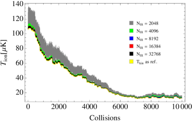
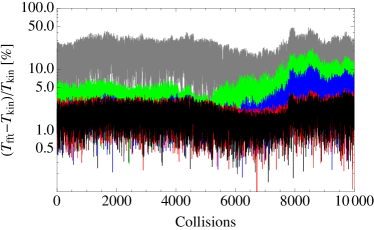
Figure 19: Average kinetic energy of a four-ion crystal colliding with thermal atoms at $2\,\mu$K (left) obtained by the Fourier method (see Eq. 38,39) The ions start at an initial temperature of around $100\,\mu$K. The Fourier spectra were obtained at different $N_{\rm{fft}}$ and a constant $\Delta t_{\rm{fft}}=50\,$ns, thus effectively varying the frequency spacing. As a reference, the temperature obtained from $\bar{E}_{\rm{kin}}$ (see Eq. 22) is shown (yellow), averaging over $8\,$ms in steps of $5\,$ns. The curves for $N_{\rm{fft}}=16384$ (red) and 32768 (black) steps are almost on top of each other, as it can be also seen in the relative deviation from $T_{\rm{kin}}$ (right).

To find a sufficient number of grid points while leaving the frequency resolution constant, we vary $\Delta t_{\rm{fft}}$ inversely with $N_{\rm{fft}}$, as shown in Fig. 20. For all combinations with $\Delta t_{\rm{fft}}\leq 200\,$ns, the relative deviation from $T_{\rm{kin}}$ is approximately the same. At $\Delta t_{\rm{fft}}=400\,$ns (gray) the maximum resolvable frequency is $f_{\rm{max}}=2.5\,$MHz, being too close to the micromotion sidebands at around $f_{\rm{rf}}=2.0\,$MHz and therefore leading to a much lower energy, dominated by only the low frequency parts. To be on the safe side, we chose the combination $\Delta t_{\rm{fft}}=50\,$ns and $N_{\rm{fft}}=16384$ for our system.

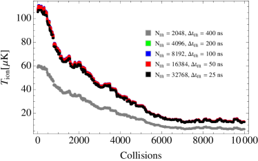
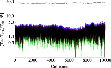
Figure 20: Average kinetic energy of a four-ion crystal colliding with atoms at $2\,\mu$K (left) obtained by the fourier method for several combinations of fourier grid sizes $N_{\rm{fft}}$ and grid spacings $\Delta t_{\rm{fft}}$, resembling a variation of the maximally resolvable frequency $f_{\rm{max}}$. All curves besides for $N_{\rm{fft}}=2048$ (gray) lie on top of each other, deviating from the average kinetic energy $T_{\rm{kin}}$ by less than 5 % (right).

While during the collision processes very fast dynamics demanding for an adaptive step size algorithm may occur, the fastest timescale during the temperature determination is set by the micromotion oscillation at $f_{\rm{rf}}=2\,$MHz in the case for $q_{z}^{2}\ll 1$. Therefore, a fixed step-size propagator with $\Delta t_{\rm{kin}}\ll 1/f_{\rm{rf}}$ is sufficient. In order to save computation time, we use the same fixed step-size propagator for the Fourier transformation energy determination as for obtaining the average kinetic energy. We therefore choose the time grid to be integer subdivisions of the Fourier grid, $\Delta t_{\rm{kin}}=\Delta t_{\rm{fft}}/n,n\in\mathbb{N}$. To find a sufficiently small $\Delta t_{\rm{kin}}$ to resolve the micromotion oscillations at $f_{\rm{rf}}=2\,$MHz, we compare the kinetic temperature as defined in Eq. 22 for different propagation time steps $\Delta t_{\rm{kin}}$ with the temperature obtained using the smallest time step $2.5\,$ns as a reference. For time steps up to $40\,$ns we obtain relative deviations of less than $0.05\,\%$ from the kinetic energy derived using time steps of $2.5\,$ns when averaged over $8\,$ms propagation time over the whole temperature range. To be on the safe side, we chose $\Delta t_{\rm{kin}}=\Delta t_{\rm{fft}}/10=5\,$ns.

Figure 21: Visualization of the normal mode movement for a trapped linear four-ion crystal in descending order with respect to the eigenmode frequency. The arrows indicate the direction and amplitude of the respective mode. The modes are shown along with their respective eigenfrequencies $f_{q_{u}}^{\rm{th}}$ obtained from the diagonalization of the secular approximation and the values $f_{q_{u}}^{\rm{fft}}$ obtained numerically from Fourier analysis of the mode spectra. Typical names of the modes are shown on the right column. The center-of-mass (c.o.m.) modes represent the upper and lower limit of the frequencies.

Appendix C Excess micromotion in a linear four-ion crystal

The obtained results for average kinetic energy and secular energy are shown in Fig. 22.

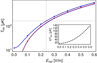
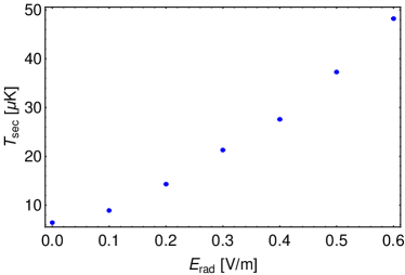
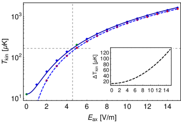
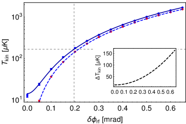
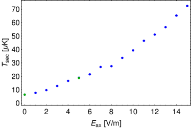
Figure 22: Average kinetic energy of a linear four-ion crystal colliding with atoms at $2\,\mu$K (left, blue) expressed as $T_{\rm{kin}}$ and temperature of the secular motion (right) versus micromotion causing parameters. The results for the kinetic energy were fit with quadratic function (solid blue curves). The dashed blue curves show the approximate theoretical amount of energy stored in the excess micromotion according to Eqs. 10, 13 and 16 respectively. The red points correspond to simulated values for the non-interacting case, in approximate agreement with the theoretical behavior. The dashed gray lines indicate the $s$-wave temperature limit. The secular part of the average kinetic energy is shown on the right. The insets show the difference between the solid and dashed blue curves, resembling the micromotion induced heating. Green points were obtained using a fixed starting/escape sphere, blue with a comoving sphere.

Each point was fit by averaging over at least 30 individual runs. The resulting average kinetic energies expressed as $T_{\rm{kin}}$ (left) follow approximately the same quadratic behavior as in the case of a single ion, indicating that the main part of the kinetic energy is stored in the micromotion. The quadratic fits (solid blue lines) lead to the increase parameters $\theta_{E_{\rm{rad}}}=7.45(3)\,\mu{\rm{K}}\cdot\left({\rm{V/m}}\right)^{-2}$, $\theta_{E_{\rm{ax}}}=2705(15)\,\mu{\rm{K}}\cdot\left({\rm{V/m}}\right)^{-2}$ and $\theta_{\delta\phi_{\rm{rf}}}=4005(16)\,\mu{\rm{K}}\cdot{\rm{mrad}}^{-2}$, in almost perfect agreement with the single ion case. For all three cases the theoretical approximate energies due to the micromotion is shown as dashed blue lines. To verify the validity of these curves, the average kinetic energy for a crystal without atoms, initialized at zero secular temperature was simulated as well (red points). Only for the case of radial excess micromotion the theoretical prediction (dashed blue) deviates significantly from the red points, indicating the approximate nature of the prediction at high radial micromotion amplitudes.

To quantify the micromotion-induced heating effect on the secular motion, the secular temperature was extracted as described in section 5. In all three cases the dependence on the scanned parameter seems to be a bit weaker than quadratic. The temperature dependence of the individual modes is discussed in section 6.4.

In all three cases, the number of collisions required to equilibrate (not shown in the figures) show a similar behavior as in the single ion case, besides the fact that they are $N_{\rm{ions}}=4$ times higher because of the reduced effective density of atoms.

References

References

- [1] Smith W W, Makarov O P and Lin J 2005 J. Mod. Opt. 52 2253–2260 URL https://doi.org/10.1080/09500340500275850
- [2] Grier A T, Cetina M, Oručević F and Vuletić V 2009 Phys. Rev. Lett. 102(22) 223201 URL https://link.aps.org/doi/10.1103/PhysRevLett.102.223201
- [3] Zipkes C, Palzer S, Sias C and Köhl M 2010 Nature 464 388 EP – URL http://dx.doi.org/10.1038/nature08865
- [4] Schmid S, Härter A and Denschlag J H 2010 Phys. Rev. Lett. 105(13) 133202 URL https://link.aps.org/doi/10.1103/PhysRevLett.105.133202
- [5] Zipkes C, Palzer S, Ratschbacher L, Sias C and Köhl M 2010 Phys. Rev. Lett. 105(13) 133201 URL https://link.aps.org/doi/10.1103/PhysRevLett.105.133201
- [6] Hall F H J, Aymar M, Bouloufa-Maafa N, Dulieu O and Willitsch S 2011 Phys. Rev. Lett. 107(24) 243202 URL https://link.aps.org/doi/10.1103/PhysRevLett.107.243202
- [7] Hall F H J and Willitsch S 2012 Phys. Rev. Lett. 109(23) 233202 URL https://link.aps.org/doi/10.1103/PhysRevLett.109.233202
- [8] Rellergert W G, Sullivan S T, Kotochigova S, Petrov A, Chen K, Schowalter S J and Hudson E R 2011 Phys. Rev. Lett. 107(24) 243201 URL https://link.aps.org/doi/10.1103/PhysRevLett.107.243201
- [9] Sullivan S T, Rellergert W G, Kotochigova S and Hudson E R 2012 Phys. Rev. Lett. 109(22) 223002 URL https://link.aps.org/doi/10.1103/PhysRevLett.109.223002
- [10] Ratschbacher L, Zipkes C, Sias C and Köhl M 2012 Nature Physics 8 649 EP – URL http://dx.doi.org/10.1038/nphys2373
- [11] Ravi K, Lee S, Sharma A, Werth G and Rangwala S A 2012 Nature Communications 3 1126 EP – URL http://dx.doi.org/10.1038/ncomms2131
- [12] Ratschbacher L, Sias C, Carcagni L, Silver J M, Zipkes C and Köhl M 2013 Phys. Rev. Lett. 110(16) 160402 URL https://link.aps.org/doi/10.1103/PhysRevLett.110.160402
- [13] Härter A and Denschlag J H 2014 Contemporary Physics 55 33–45 URL https://doi.org/10.1080/00107514.2013.854618
- [14] Hall F H, Eberle P, Hegi G, Raoult M, Aymar M, Dulieu O and Willitsch S 2013 Molecular Physics 111 2020–2032 URL https://doi.org/10.1080/00268976.2013.780107
- [15] Haze S, Saito R, Fujinaga M and Mukaiyama T 2015 Phys. Rev. A 91(3) 032709 URL https://link.aps.org/doi/10.1103/PhysRevA.91.032709
- [16] Meir Z, Sikorsky T, Ben-shlomi R, Akerman N, Dallal Y and Ozeri R 2016 Phys. Rev. Lett. 117(24) 243401 URL https://link.aps.org/doi/10.1103/PhysRevLett.117.243401
- [17] Saito R, Haze S, Sasakawa M, Nakai R, Raoult M, Da Silva H, Dulieu O and Mukaiyama T 2017 Phys. Rev. A 95(3) 032709 URL https://link.aps.org/doi/10.1103/PhysRevA.95.032709
- [18] Tomza M, Jachymski K, Gerritsma R, Negretti A, Calarco T, Idziaszek Z and Julienne P S 2017 ArXiv e-prints (Preprint 1708.07832)
- [19] Krych M, Skomorowski W, Pawłowski F, Moszynski R and Idziaszek Z 2011 Phys. Rev. A 83(3) 032723 URL https://link.aps.org/doi/10.1103/PhysRevA.83.032723
- [20] Krych M and Idziaszek Z 2015 Phys. Rev. A 91 023430
- [21] Kollath C, Köhl M and Giamarchi T 2007 Phys. Rev. A 76(6) 063602 URL https://link.aps.org/doi/10.1103/PhysRevA.76.063602
- [22] Doerk H, Idziaszek Z and Calarco T 2010 Phys. Rev. A 81(1) 012708 URL https://link.aps.org/doi/10.1103/PhysRevA.81.012708
- [23] Secker T, Gerritsma R, Glaetzle A W and Negretti A 2016 Phys. Rev. A 94(1) 013420 URL https://link.aps.org/doi/10.1103/PhysRevA.94.013420
- [24] Bissbort U, Cocks D, Negretti A, Idziaszek Z, Calarco T, Schmidt-Kaler F, Hofstetter W and Gerritsma R 2013 Phys. Rev. Lett. 111(8) 080501 URL https://link.aps.org/doi/10.1103/PhysRevLett.111.080501
- [25] Idziaszek Z, Calarco T, Julienne P S and Simoni A 2009 Phys. Rev. A 79(1) 010702 URL https://link.aps.org/doi/10.1103/PhysRevA.79.010702
- [26] Idziaszek Z, Simoni A, Calarco T and Julienne P S 2011 New Journal of Physics 13 083005 URL http://stacks.iop.org/1367-2630/13/i=8/a=083005
- [27] Tomza M, Koch C P and Moszynski R 2015 Phys. Rev. A 91(4) 042706 URL https://link.aps.org/doi/10.1103/PhysRevA.91.042706
- [28] Gacesa M and Côté R 2017 Phys. Rev. A 95(6) 062704 URL https://link.aps.org/doi/10.1103/PhysRevA.95.062704
- [29] Fürst H, Feldker T, Vincenz Ewald N, Joger J, Tomza M and Gerritsma R 2017 ArXiv e-prints (Preprint 1712.07873)
- [30] Chin C, Grimm R, Julienne P and Tiesinga E 2010 Rev. Mod. Phys. 82(2) 1225–1286 URL https://link.aps.org/doi/10.1103/RevModPhys.82.1225
- [31] Bloch I, Dalibard J and Nascimbène S 2012 Nature Physics 8 267 EP – URL http://dx.doi.org/10.1038/nphys2259
- [32] Major F G and Dehmelt H G 1968 Phys. Rev. 170(1) 91–107 URL https://link.aps.org/doi/10.1103/PhysRev.170.91
- [33] DeVoe R G 2009 Phys. Rev. Lett. 102(6) 063001 URL https://link.aps.org/doi/10.1103/PhysRevLett.102.063001
- [34] Zipkes C, Ratschbacher L, Sias C and Köhl M 2011 New Journal of Physics 13 053020 URL http://stacks.iop.org/1367-2630/13/i=5/a=053020
- [35] Cetina M, Grier A T and Vuletić V 2012 Phys. Rev. Lett. 109(25) 253201 URL https://link.aps.org/doi/10.1103/PhysRevLett.109.253201
- [36] Chen K, Sullivan S T and Hudson E R 2014 Phys. Rev. Lett. 112(14) 143009 URL https://link.aps.org/doi/10.1103/PhysRevLett.112.143009
- [37] Ewald N V 2015 Quest for an Ultracold Hybrid Atom-Ion Experiment Master’s thesis Johannes Gutenberg-Universität Mainz
- [38] Höltkemeier B, Weckesser P, López-Carrera H and Weidemüller M 2016 Phys. Rev. Lett. 116(23) 233003 URL https://link.aps.org/doi/10.1103/PhysRevLett.116.233003
- [39] Höltkemeier B, Weckesser P, López-Carrera H and Weidemüller M 2016 Phys. Rev. A 94(6) 062703 URL https://link.aps.org/doi/10.1103/PhysRevA.94.062703
- [40] Rouse I and Willitsch S 2017 Phys. Rev. Lett. 118(14) 143401 URL https://link.aps.org/doi/10.1103/PhysRevLett.118.143401
- [41] Secker T, Ewald N, Joger J, Fürst H, Feldker T and Gerritsma R 2017 Phys. Rev. Lett. 118(26) 263201 URL https://link.aps.org/doi/10.1103/PhysRevLett.118.263201
- [42] Leibfried D, Blatt R, Monroe C and Wineland D 2003 Rev. Mod. Phys. 75(1) 281–324 URL https://link.aps.org/doi/10.1103/RevModPhys.75.281
- [43] Berkeland D J, Miller J D, Bergquist J C, Itano W M and Wineland D J 1998 Journal of Applied Physics 83 5025–5033 URL https://doi.org/10.1063/1.367318
- [44] Meir Z 2016 Dynamics of a single, ground-state cooled and trapped ion colliding with ultracold atoms: A micromotion tale. Ph.D. thesis Weizmann Institute of Science
- [45] Meir Z, Sikorsky T, Ben-shlomi R, Akerman N, Pinkas M, Dallal Y and Ozeri R 2018 Journal of Modern Optics 65 501–519 URL https://doi.org/10.1080/09500340.2017.1397217
- [46] Langevin M P 1905 Annales de Chimie et de Physique, series 5 245–288 URL https://ci.nii.ac.jp/naid/10004043377/en/
- [47] Weisstein E W 2002 Sphere point picking URL http://mathworld.wolfram.com/SpherePointPicking.html
- [48] Press W H 2007 Numerical recipes 3rd edition: The art of scientific computing (Cambridge university press)
- [49] Joger J, Fürst H, Ewald N, Feldker T, Tomza M and Gerritsma R 2017 Phys. Rev. A 96(3) 030703(R) URL https://link.aps.org/doi/10.1103/PhysRevA.96.030703
- [50] Olmschenk S, Younge K C, Moehring D L, Matsukevich D N, Maunz P and Monroe C 2007 Phys. Rev. A 76(5) 052314 URL https://link.aps.org/doi/10.1103/PhysRevA.76.052314
- [51] Taylor P, Roberts M, Gateva-Kostova S V, Clarke R B M, Barwood G P, Rowley W R C and Gill P 1997 Phys. Rev. A 56(4) 2699 URL https://link.aps.org/doi/10.1103/PhysRevA.56.2699
- [52] James D 1998 Applied Physics B 66 181–190 ISSN 1432-0649 URL https://doi.org/10.1007/s003400050373
- [53] Cooley J W and Tukey J W 1965 Mathematics of Computation 19 297–301 ISSN 00255718, 10886842 URL http://www.jstor.org/stable/2003354
- [54] Lemmer A, Cormick C, Schmiegelow C T, Schmidt-Kaler F and Plenio M B 2015 Phys. Rev. Lett. 114(7) 073001 URL https://link.aps.org/doi/10.1103/PhysRevLett.114.073001
- [55] Kaufmann H, Ulm S, Jacob G, Poschinger U, Landa H, Retzker A, Plenio M B and Schmidt-Kaler F 2012 Phys. Rev. Lett. 109(26) 263003 URL https://link.aps.org/doi/10.1103/PhysRevLett.109.263003
- [56] Landa H, Drewsen M, Reznik B and Retzker A 2012 New Journal of Physics 14 093023 URL http://stacks.iop.org/1367-2630/14/i=9/a=093023
- [57] Shen C and Duan L M 2014 Phys. Rev. A 90(2) 022332 URL https://link.aps.org/doi/10.1103/PhysRevA.90.022332
- [58] Richerme P 2016 Phys. Rev. A 94(3) 032320 URL https://link.aps.org/doi/10.1103/PhysRevA.94.032320
- [59] Serwane F, Zürn G, Lompe T, Ottenstein T B, Wenz A N and Jochim S 2011 Science 332 336–338 ISSN 0036-8075 URL http://science.sciencemag.org/content/332/6027/336
- [60] Gross C, Gan H C J and Dieckmann K 2016 Phys. Rev. A 93(5) 053424 URL https://link.aps.org/doi/10.1103/PhysRevA.93.053424