The acceleration relation in galaxies and scale invariant dynamics: another challenge for dark matter

Abstract

We examine the radial acceleration relation (RAR) between the centripetal acceleration $g_{\mathrm{obs}}$ and the gravity due to the baryons $g_{\mathrm{bar}}$ in galaxies (McGaugh et al., 2016; Lelli et al., 2017). Below about $10^{-10}$ m s^-2, the RAR deviates from the 1:1 line, $g_{\mathrm{obs}}$ being much larger than $g_{\mathrm{bar}}$. The RAR is followed by late and early type galaxies, and also by the dwarf spheroidals where the deviations from the 1:1 line are the largest ones. These deviations are currently attributed to dark matter.

We show that the scale invariant theory, with the assumption of the scale invariance of the empty space, correctly predicts the observed deviations in the acceleration relation. The large deviations (up to a factor 400) and the flattening of the acceleration relation observed for the dwarf spheroidal galaxies are also well described. The presence of dark matter is no longer necessary in the scale invariant context, which also accounts why dark matter usually appears to dominate in regions of late type galaxies with low baryonic gravities.

1 Introduction: the context

The relation between the dynamics of galaxies and the distributions of their visible matter opened a large variety of studies on the dark matter and gravitation (Sofue and Rubin, 2001). The radial acceleration relation (RAR) compares the radial acceleration traced by the rotation curves of galaxies and the acceleration expected from the observed distribution of baryons (McGaugh, 2004). It is also often expressed in terms of a mass discrepancy acceleration relation (MDAR). Recent extensions of this relation to different types of galaxies have been performed by McGaugh et al. (2016) and Lelli et al. (2017). Their conclusion is that the dark matter (DM) distribution is fully determined by that of the baryons or vice-versa. A number of authors have interpreted this relation in the context of the $\Lambda$CDM models of galaxy formation, in terms of different mass-dependent density profiles of DM haloes (Di Cintio and Lelli, 2016), of simulations of galaxy formation matching the velocities and the scaling relations (Santos-Santos, 2016), in particular if stellar masses and sizes are closely related to the masses and sizes of their DM haloes (Navarro et al., 2017). Keller and Wadsley (2017) show that the account for the hot outflows from supernovae at high $z$ improves the comparisons by producing a baryon depletion, while the effects of the AGN feedback is considered by Ludlow et al. (2017). The role of the galaxy-halo connexion is also emphasized by Desmond (2017). Attempts to explain the observed relation in the context of modified gravity (MOND) have been made by Milgrom (2016) and Li et al. (2018).

New cosmological models have recently been proposed, which include the specific hypothesis that the macroscopic empty space is invariant to a scale transformation, a property absent from general relativity (GR) with a cosmological constant, but present in the Maxwell equations (Maeder, 2017a). These models are based on the general field equation in Weyl’s geometry obtained by Dirac (1973) and Canuto et al. (1977), which includes also the possibility of scale invariance in addition to the general covariance of GR. These models predict an accelerated cosmic expansion without advocating the existence of some unknown form of dark energy. Several comparisons between models and observations have been performed: on the distance vs. redshifts, the $m-z$ diagram, the $\Omega_{\Lambda}$ vs. $\Omega_{\mathrm{m}}$ plot, the age vs. $H_{0}$, the expansion rate $H(z)$ vs. redshifts $z$ and on the redshift of the transition from braking to the present acceleration of the cosmic expansion. A critical analysis of the CMB temperatures as function of $z$ from CO molecules in DLA is also supporting these cosmological models (Maeder, 2017b).

The scale invariant models also have consequences for weak gravitational fields. A geodesic equation in the scale invariant framework was obtained by Bouvier and Maeder (1978). Applied to a weak field, the relation corresponding to Newton’s law was derived. It contains an additional small acceleration term proportional to the velocity, particularly significant in low gravity and low density regions (Maeder and Bouvier, 1979; Maeder, 2017c). This leads to an energy relation, which for clusters of galaxies provides mass determinations much smaller than usual, letting little or no room for dark matter. A detailed study of the two-body problem has also been made in the scale invariant framework. This allows, alike the MOND theory (Milgrom, 1983), but in a more general context, to account for the flat rotation curve of the Milky Way and galaxies (Sofue and Rubin, 2001; Sohn et al., 2017), and also why no dark matter is suggested in forming galaxies at redshifts around z =2 (Wuyts et al., 2016; Genzel et al., 2017; Lang et al., 2017).

Here, we want to check whether the RAR or MDAR can be interpreted within the scale invariant framework. In Section 2, after an additional demonstration of the gauging condition, the acceleration relation is studied in the scale invariant context. In Section 3, the observations and predictions of the scale invariant theory are compared. Section 4 presents a discussion about dark matter and on some possibilities to distinguish between the $\Lambda$CDM and the scale invariant theories. Conclusions are given in Section 5.

2 The radial acceleration relation in the scale invariant theory

2.1 The models and the gauging conditions

The models studied here are based on the theoretical developments made by Weyl (1923); Eddington (1923); Dirac (1973); Canuto et al. (1977) and Bouvier and Maeder (1978) for a gravitation theory including scale invariance in addition to the general covariance. A scale transformation of the line element $ds^{\prime}$ of GR is expressed by

$$ds^{\prime}=\lambda(x^{\mu})ds\,$$ (1)

where $ds$ is a new line element. Weyl’s Geometry, instead of Riemann Geometry, offers the consistent framework, in which scale invariance can be expressed in addition to the general covariance of GR. Dirac and later Canuto et al. have expressed in the scale invariant framework an action principle, which includes a matter Lagrangian as a coscalar of power -4. In the integrable Weyl’s space, Dirac and Canuto et al. have shown that the scale factor remains undetermined without any other constraints. Later, they were fixing the scale factor by some external considerations based on the large number hypothesis (instead of that we fix it by an assumption on the vacuum property). From the differential of the action, a generalization of the Einstein field equation satisfying both general covariance and scale invariance was obtained. This is Equation (7) used in the paper by Maeder (2017a). This field equation can also be derived in the step by step developments of the so-called cotensor calculus, which is the basic mathematical tool of Weyl’s geometry, like tensor calculus in Riemann Geometry. Scale covariant derivatives, modified Christoffel symbols, the Riemann-Christoffel tensor also have their scale covariant counterparts. A short summary on cotensors has been given by Canuto et al. (1977).

The contribution by Bouvier and Maeder was to obtain the geodesic equation, expressing the motion of a free particle from a minimum action expressing the shortest distance between two points in the integrable Weyl’s space. A derivation of the geodesic equation from the Equivalence Principle was further given by Maeder and Bouvier (1979). They also showed that this geodesic equation leads to a slightly modified Newton’s equation, see below Equation (10) (Maeder, 2017c). Thus, both the general field equation and the geodesic equation in the scale invariant context used in the previous papers have been thoroughly studied and analyzed in the cotensor framwork and from an action principle.

In Equation (1), $\lambda$ is the scale factor, which for reasons of homogeneity and isotropy only depends on time. The ”new” general field and geodesic equations contain terms depending on the coefficient of metrical connection $\kappa_{\nu}$,

$$\kappa_{\mu}\,=\,-\frac{\partial}{\partial x^{\mu}}\,\ln\lambda\,.$$ (2)

and its derivatives. The geodesic equation writes,

$$\frac{du^{\rho}}{ds}+\Gamma^{\rho}_{\mu\nu}u^{\mu}u^{\nu}-\kappa_{\mu}u^{\mu}u^{\rho}+\kappa^{\rho}=0\,,$$ (3)

with the velocity $u^{\mu}\,=\,dx^{\mu}/ds$. It contains two additional terms depending on $\kappa_{\mu}$. Interestingly enough, for $\kappa_{\mu}$ given by Equation (2), any vector undergoing a parallel displacement along a closed curve has its length unchanged in Weyl’s space, alike in Riemann space, while this would not be the case for other forms of $\kappa_{\mu}$. Other properties of Weyl’s geometry define a consistent framework for gravitation (Bouvier and Maeder, 1978).

It is often not realized that Einstein’s field equation in GR is scale invariant, when the cosmological constant $\Lambda_{\mathrm{E}}$ is equal to zero. However, the point is that the property of scale invariance is no longer verified, when the cosmological constant is different from zero (Bond, 1990). The specific hypothesis we have made to the fix the gauge $\lambda$ (Maeder, 2017a) is that the macroscopic empty space should be invariant to a scale transformation even if the cosmological constant is different from zero. In this respect, we recall that the Maxwell equations are also scale invariant in the empty space. When this hypothesis is expressed in the general scale invariant field equation, it leads to two differential equations between the scale factor $\lambda(t)$, its derivatives and the cosmological constant $\Lambda_{\mathrm{E}}$ (Maeder and Bouvier, 1979; Maeder, 2017a),

$$\ 3\,\frac{\dot{\lambda}^{2}}{\lambda^{2}}\,=\,\lambda^{2}\,\Lambda_{\mathrm{E}}\,,$$ (4)

$$\frac{\ddot{\lambda}}{\lambda}\,=\,2\,\frac{\dot{\lambda}^{2}}{\lambda^{2}}\,,$$ (5)

or some combination of the two. The solution of these equations gives $\lambda$ varying like $1/t$. Thanks to these relations $\Lambda_{\mathrm{E}}$ can be eliminated from the cosmological equations and a fully determined system of equations is obtained for the chosen metric. Interestingly enough, the above relations bring major simplifications in the cosmological equations by Canuto et al. (1977).

Now, let us examine more closely the meaning of the above relations between the cosmological constant and the scale factor $\lambda$. The cosmological constant is related by some constant factor to the energy density $\varrho_{v}$ of the empty space, see for example Carroll et al. (1992),

$$\Lambda_{\mathrm{E}}\,=\,8\pi\,G\,\varrho_{v}\,,$$ (6)

with $c=1$. Let $\ell^{\prime}$ be a constant line element in the space of GR. In the scale invariant space, the line element becomes $\ell\,=\frac{\ell^{\prime}}{\lambda(t)}$, where $\lambda$ is only a function of the cosmic time $t$, as said above. The possible variations of the scale factor $\lambda$ may contribute to the energy density present in the empty space. Thus, if $\lambda(t)$ varies, the energy density present in the empty space will depend on $\dot{\ell}^{2}\,=\,\ell^{\prime 2}\,\frac{\dot{\lambda}^{2}}{\lambda^{4}}.$ If there is no other source of energy in the macroscopic empty space, the cosmological constant is thus proportional to $\dot{\ell}^{2}$,

$$\Lambda_{\mathrm{E}}\,=\,const.\frac{\dot{\lambda}^{2}}{\lambda^{4}}\,,$$ (7)

which compares with Equation (4). The cosmological constant $\Lambda_{\mathrm{E}}$ is a true constant and this implies,

$$\frac{d\Lambda_{\mathrm{E}}}{dt}\,=\,0\,\quad\Longrightarrow\quad\frac{d\dot{\ell}^{2}}{dt^{2}}=2\dot{\ell}\,\ddot{\ell}\,=\,\ell^{\prime 2}\left(\frac{\dot{\lambda}\ddot{\lambda}}{\lambda^{4}}-2\,\frac{\dot{\lambda}^{3}}{\lambda^{5}}\right)\,=\,0\,.$$ (8)

Expressing $\ddot{\ell}$, we get $\ddot{\ell}\,=\,\frac{\ell^{\prime}}{\lambda}\left(\frac{\ddot{\lambda}}{\lambda}-2\,\frac{\dot{\lambda}^{2}}{\lambda^{2}}\right)$. The second derivative of $\ell$ should be zero in order to satisfy Equation (8) for $\dot{\ell}\neq\,0$, thus

$$\ddot{\ell}\,=\,0,\quad\Longrightarrow\quad\frac{\ddot{\lambda}}{\lambda}\,=\,2\,\frac{\dot{\lambda}^{2}}{\lambda^{2}}\,,$$ (9)

in agreement with Equation (5). We see that the gauging conditions, independently obtained 1) from the hypothesis of scale invariance of the empty space and 2) from the constancy of the energy density of the empty space are both giving identical results. This confirms the consistency of the adopted gauging condition. In GR, the cosmological constant, and thus the density of the empty space, is independent of the material content of the Universe. This also applies to the conditions (4) and (5) expressing the energy–density of the empty space in terms of the scale factor. In this framework, the only significant energy in the large scale empty space is that resulting from the gauge variations. Indeed, we consider this applies to large scales, even if this is not necessarily true at the quantum level, in the same way as we may use Einstein theory at large scales, even if we cannot do it at the quantum level.

With the Robertson-Walker metric, the above gauging conditions (4) and (5) enabled us to express the cosmological equations (29) - (31) in Maeder (2017a). The resulting models predict an acceleration of the cosmic expansion and satisfy various cosmological tests.

2.2 Some basic useful relations in the scale invariant context

The above scale invariant equation of the geodesics applied in the weak field approximation is leading to a modified form of the Newton equation (Maeder and Bouvier, 1979; Maeder, 2017c),

$$\frac{d^{2}\mathbb{r}}{dt^{2}}\,=\,-\frac{G\,M}{r^{2}}\,\frac{\mathbb{r}}{r}+\,\kappa(t)\,\frac{d\mathbb{r}}{dt}\,,$$ (10)

where $\kappa(t)\,=\,1/t$ with $t$ being the cosmic time. In addition to the usual gravitational attraction it contains a small acceleration term proportional the velocity, particularly significant in low gravity and low density media (Section 2.4). The additional term results from the cosmological constant, which is related to the scale factor $\lambda$ and its first derivative by Equation (4). For a constant scale factor $\lambda$, there is no acceleration term. The law of conservation of angular momentum $L$ is different from the usual one,

$$\kappa(t)\,r^{2}\,\dot{\vartheta}\,=\,L\,=\,\mathrm{const.}$$ (11)

It is a scale invariant quantity. The equation of motion (10) has been applied to the two-body problem and an equivalent form to Binet equation has been found. The orbits $r(\vartheta)$ belong to the usual family of conics, with in addition a slight outward expansion motion,

$$r\,=\,\frac{r_{0}}{1+e\cos(\vartheta)},\quad\mathrm{with}\quad r_{0}\,=\,\frac{L^{2}}{G\,M\,\kappa^{2}(t)}\,,$$ (12)

where $r_{0}$ is the radius of the circular orbit. The eccentricity $e$ is scale invariant, while $r_{0}$ varies like $t$. The circular velocity in the case of the two-body problem is according to Equation (11) $v_{\mathrm{c}}\,=\,r_{0}\,\dot{\vartheta}\,=\,\frac{L}{\kappa(t)\,r_{0}}$, which is also a scale invariant quantity. Now, with the expression (12) for $r_{0}$, one obtains

$$v^{2}_{\mathrm{c}}\,=\frac{G\,M}{r_{0}}\,.$$ (13)

The expression relating the circular velocity and the gravitational potential is valid. Consistently, the gravitational potential is also a scale invariant quantity, since we have both $r^{\prime}=\lambda r$ and $M^{\prime}=\lambda M$, as already seen in Maeder (2017a). For an elliptical motion, the semi-major axis $a$ and the period $P$ also behave like $\dot{a}/a=\dot{P}/P=1/t$. These relations illustrate the main properties of the motions. The additional outward acceleration term in Equation (10) does not produce a change of the circular velocity, but just an extension of the orbit and a corresponding reduction of the angular velocity.

2.3 Energy relation in the scale invariant context

A gravitational system governed by Equation (10) does not reach a state of perfect equilibrium in the long term, since the additional term produces secular variations of the orbits. The additional term in this equation does not derive from a potential, thus the conditions are different from those of the usual virial theorem. Since the variations of the orbits due to the additional term are currently slow, a gravitational system may find a state of quasi-equilibrium. Thus, we may find an expression which relates the different forms of energy present. Let us consider the ensemble of $N$ stars moving in a galaxy. According to Eq.(10), the acceleration of a star $i$ interacting with another one of mass $m_{j}$ is

$$\frac{dv_{ij}}{dt}\,=\,-\frac{G\,m_{j}}{r^{2}_{ij}}+\kappa(t)\,v_{ij}\,\,,$$ (14)

where $r_{ij}$ is the distance between objects $i$ and $j$ and $v_{ij}=\frac{dr_{ij}}{dt}$. First, we multiply this equation by $v_{ij}$ and get

$$\frac{1}{2}d(v^{2}_{ij})\,=\,-\frac{G\,m_{j}}{r^{2}_{ij}}\,dr_{ij}+\kappa(t)\,v^{2}_{ij}dt\,,$$ (15)

Summing on all the interactions of the $j\neq i$ stars with the one noted $i$, then summing on all the $i$ stars, we get

$$\frac{1}{2}\sum_{i}\sum_{j\neq i}d(v^{2}_{ij})\,=\,-\sum_{i}\sum_{j\neq i}\frac{G\,m_{j}}{r^{2}_{ij}}\,dr_{ij}+\sum_{i}\sum_{j\neq i}\kappa(t)\,v^{2}_{ij}dt\,,$$ (16)

The square of the velocity of the $i$ star due to its interactions with all the $j$ ones is $\frac{1}{N}\sum_{j\neq i}v^{2}_{ij}$. In the double summations, each of the $N(N-1)/2$ interactions is counted twice. To get the mean values, we divide the double summations by $N(N-1)$, ($N$ being very large, $N(N-1)\approx N^{2}$) and obtain

$$d(\overline{v^{2}})\,\approx\,-q^{\prime}\frac{GM}{R^{2}}dR+2\,\kappa(t)\overline{v^{2}}dt\,,$$ (17)

where $M$ and $R$ are the mass and radius of the configuration and $q^{\prime}$ is a structural factor of the order of unity, as discussed below. The terms $\frac{G\,m_{j}}{r^{2}_{ij}}\,dr_{ij}$ is scale invariant since the effects of a change of scale act the same way on masses and radii. The above expression is then integrated between time $t_{\mathrm{in}}$, the time of the galaxy formation and the present time $t_{0}$. (As the analyzed galaxies have small redshifts, it is like if they are observed at present.)

At some stage in the process of galaxy formation, the infall of matter was locally stopped by the centrifugal or pressure forces. Let us call $t_{\mathrm{in}}$ the time when this state of quasi-equilibrium occured. At this time, since the infall velocity vanishes, the effects of the slow secular term (which depends on the velocity) become negligible in the balance between the centrifugal force and Newtonian attraction. (We may however notice that this stage of quasi-equilibrium with a vanishing infall velocity does likely not occur at the same time for all galactocentric radii. However, in the present estimate we do not account for this fact, considering that the spread in the formation times at different radii is small with respect to the age of the galaxies. Moreover, as the present derivation is only applied to the dwarf spheroidals (Section 3.2), the approximation appears rather justified.) With account of these remarks, after integration we get the following energy equation,

$$\overline{v^{2}}\,\approx\,q^{\prime}\frac{G\,M}{R}+2\,\int^{t_{0}}_{t_{\mathrm{in}}}\kappa(t)\,\overline{v^{2}(t)}\,dt\,.$$ (18)

The value of $\overline{v^{2}}$ is the average of the present velocities, $M$ and $R$ are the present values. We see that the non-Newtonian term on the right side leads to cumulative contributions over the ages. This effect is not present in the models of cold dark matter ($\Lambda$CDM model) and this may thus give some tests of the different theories (Section 4.2).

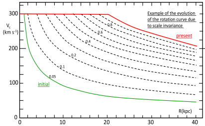
Figure 1: Example of the evolution of the rotation curve of a galaxy in the scale invariant theory. The initial curve in green corresponds to to a time $t=0.05\,t_{0}$, the present curve in red is that for $t_{0}=1$. At a given value of the radius $R$ in kpc, the square of the circular velocity is defined by Equation (13).

Let us try to express the above equation as a function of the gravities used by Lelli et al. (2017). The approximation is made,

$$2\,F\,\equiv\,2\,\int^{t_{0}}_{t_{\mathrm{in}}}\kappa(t)\,\overline{v^{2}(t)}\,dt\,\approx\,2\,f\,\frac{\overline{v^{2}(t_{0})}}{t_{0}}\,\Delta t\,.$$ (19)

The factor $f$ is a numerical factor of the order of unity, discussed below. The interval of time $\Delta t$ is equal to the total distance $\Delta r$ covered by a typical star during its circular motions at a constant circular velocity $\overline{v_{\mathrm{circ}}}$, thus $\Delta t\approx\Delta r/\overline{v_{\mathrm{circ}}}$. The total distance $\Delta r$ is given by the number $n$ of circular orbits that a representative star has described during its lifetime, thus $\Delta r\approx n\times 2\,\pi\,\overline{R}$, where $\overline{R}$ is a time average of the typical radius. The values of $n$ may be of the order of a few tens. The present circular velocity is $v_{\mathrm{circ}}\,=\,(g_{\mathrm{obs}}\,R)^{1/2}$. According to Equation (13), it is an invariant. The approximation $\overline{R}\approx(1/2)R$ is taken. This leads to

$$2\,F\,\approx\,2f\,\frac{\overline{v^{2}}}{t_{0}}\,\frac{2\pi n\overline{R}}{(g_{\mathrm{obs}}\,R)^{1/2}}\,\approx\,2f\,\frac{\overline{v^{2}}}{t_{0}}\,n\pi\left(\frac{R}{g_{\mathrm{obs}}}\right)^{\frac{1}{2}}\,.$$ (20)

The energy equation (18) then becomes

$$g_{\mathrm{obs}}\,\left[1-\frac{2fn\pi}{t_{0}}\left(\frac{R}{g_{\mathrm{obs}}}\right)^{\frac{1}{2}}\right]\,\approx\ q^{\prime}\,g_{\mathrm{bar}}\,.$$ (21)

The mean gravitational acceleration $\frac{G\,M}{R^{2}}$ at some galactocentric distance $R$ encompassing a mass $M$ gives $g_{\mathrm{bar}}$. The estimate of $g_{\mathrm{obs}}$ is based on $\overline{v^{2}}/R$, the observed velocity being obtained by the projection of the total velocity.

This relation contains several approximations. 1.- The first is the structural factor $q^{\prime}$. The value of $q^{\prime}$ is $q^{\prime}=6/5$ for a constant spherical distribution and $q^{\prime}=4/3$ for a disk of constant density. For an almost linearly regularly decreasing density with a polytropic index $n=1$, $q^{\prime}=3/2$. Uncertainties on $q^{\prime}$ may affect the values of $\log g_{\mathrm{bar}}$, however they are at most of the order of one or two tenths of dex. In fact, this uncertainty disappears in the plot, since an appropriate mass-luminosity ratio is applied so that the observed $\log g_{\mathrm{bar}}$ and $\log g_{\mathrm{obs}}$ are equal for the highest gravities in the galaxy sample by Lelli et al. (2017).

2.- Another uncertainty concerns the factor $f$, expressing the mean of $\frac{v^{2}}{t}$ over the galaxy lifetime $\Delta t$. The main effect of scale invariance is the progressive radial expansion of a rotating galaxy keeping a constant circular velocity $v_{\mathrm{circ}}$. Fig. 1 gives an example of a dynamical evolution consistent with the above equations, (see Fig. 2 in Maeder (2017c)). At a given radius $r$, the circular velocity at time $t$ is given by

$$v_{\mathrm{circ}}(t)\,=\,v_{0}\left(\frac{r_{\mathrm{flat}}(t_{\mathrm{in}})}{r}\,\frac{t}{t_{\mathrm{in}}}\right)^{1/2}\,,$$ (22)

where $r_{\mathrm{flat}}(t_{\mathrm{in}})$ is the radius up to which the velocity is about constant ($v_{0}$) at the initial time $t_{\mathrm{in}}$. The velocity $v_{\mathrm{circ}}(t)$ cannot be larger than $v_{0}$. At a given $r$, the value of $v^{2}_{\mathrm{circ}}$ grows linearly with time until it reaches $v^{2}_{0}$. The integral $\int^{t_{0}}_{t_{\mathrm{in}}}\kappa(t)\,\overline{v^{2}(t)}\,dt=v^{2}_{0}\left(\frac{t_{-}t_{\mathrm{in}}}{t_{0}}\right)$ and thus is smaller than 1. If $t_{0}>\frac{r}{r_{\mathrm{flat}}}t_{\mathrm{in}}$ the velocity is constant and the integral becomes slightly larger than 1. On the whole, $f\approx 1$ appears an acceptable approximation.

3.- The mean radius $\overline{R}$ of an orbit during the galactic lifetime has also been approximated. As the radius of an orbit grows linearly in time, the mean radius over the time $(t_{0}-t_{\mathrm{in}})$ is $\overline{R}=0.55\;R$ or $0.525$, if the initial time is equal to 10% or 5% of the present time respectively. Thus, the approximations made appear acceptable in this analytical approach of a complex problem to be further studied by detailed numerical computations.

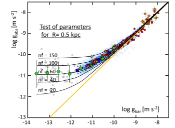
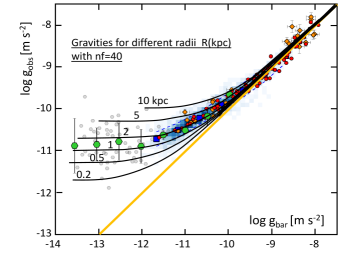
Figure 2: Left:The acceleration relation for all galaxies studied from Fig. 12 left by Lelli et al. (2017), with continuous black lines derived from Equation (21) for different values of the product $nf$. A reference value of $R=0.5$ kpc is taken. The blue squares represent the binned data for 153 LTGs, the thin blue broken lines indicate the standard deviation around their average. The rotating ETGs are represented by red circles, and the X-ray ETGs by orange diamonds. The small grey hexagons show the dwarf spheroidals, while the large green hexagons give their mean values. Vertical and horizontal bars show standard deviations. The yellow line shows the relation where the two gravities are equal. Right: the same for $nf=40$ and different radii.

Fig. 2 (left) shows the results for a radius $R=0.5$ kpc with different values of $nf$. For the high gravities, all the curves are close to the 1:1 yellow line and thus the main constraints come from the low gravity objects which show the largest deviations, in particular the spheroidal galaxies. Fig. 2 right shows the curves for $nf=60$ and different radii. The general distribution and the flattening for low gravities are well reproduced. The flattening results from the fact that for lower values of $g_{\mathrm{obs}}$ the parenthesis in Equation (21) becomes very small. The predicted curves tend toward a horizontal asymptotic line, in agreement with the general trend discovered by Lelli et al. (2017).

In the plot of the RAR of the LTGs and ETGs, there is a full mixture of values of $R$ and velocities along the sequence of observations, since a given value of $g_{\mathrm{obs}}$ can be realized by a wide combination of velocities and radii. This prevents the application of the above developments to this sample. However, in the case of the spheroidals, the situation is more favorable since at a given mean $g_{\mathrm{obs}}$ we have a defined mean radius, as seen in Section (3.2).

2.4 Relation between gravities and densities

For the LTGs and ETGs, we need a relation between $g_{\mathrm{obs}}$ and $g_{\mathrm{bar}}$ which does not depend on the radius or velocity of the observations. The second term in brackets in Equation (21), which is responsible for the deviations from the 1:1 line in the gravity plot, results from the additional dynamical term in the equation of motion (10) integrated over the time. The ratio $x$ at a given time $t$ of the additional term in Equation (10) to the classical Newtonian term behaves like

$$x\,=\,\frac{v\,r^{2}}{GM\,t}\,\approx\,\sqrt{2}\,\left(\frac{\varrho_{\mathrm{c}}}{\overline{\varrho}}\right)^{1/2}\,,$$ (23)

as shown by Maeder (2017c). There $\overline{\varrho}$ is the mean density of the considered configuration and $\varrho_{\mathrm{c}}$ the classical critical density of the Universe at time $t$. The ratio $x$ is a scale invariant term. For a disk galaxy of thickness $h$, the average density is

$$\overline{\varrho}\,=\,\frac{M}{4\pi R^{2}h}\,=\,\frac{g_{\mathrm{bar}}}{4\pi Gh}\,,$$ (24)

where $M$ is the mass inside radius $R$ and $g_{\mathrm{bar}}$ the local baryonic gravity. For LTGs of a given thickness as considered by Lelli et al. (2017), the gravities and mean densities are proportional to each other. Thus, the expression of $x$ shows that for LTGs the dynamical effects resulting from the non-Newtonian term are proportional to $g_{\mathrm{bar}}^{-(1/2)}$.

In the plot $\log g_{\mathrm{obs}}$ vs. $\log g_{\mathrm{bar}}$, the deviations of $\log g_{\mathrm{obs}}$ from the 1:1 line result from these effects integrated over the ages. Thus, at two different baryonic gravities $g_{\mathrm{bar,1}}$ and $g_{\mathrm{bar,2}}$ for galaxies assumed to be of similar ages, the relative differences $\left(\frac{g_{\mathrm{obs}}-g_{\mathrm{bar}}}{g_{\mathrm{bar}}}\right)$ should behave like,

$$\frac{\left(\frac{g_{\mathrm{obs}}-g_{\mathrm{bar}}}{g_{\mathrm{bar}}}\right)_{2}}{\left(\frac{g_{\mathrm{obs}}-g_{\mathrm{bar}}}{g_{\mathrm{bar}}}\right)_{1}}\,=\,\left(\frac{g_{\mathrm{bar,1}}}{g_{\mathrm{bar,2}}}\right)^{1/2}\,.$$ (25)

Globally the deviations from the 1:1 line in the gravity plot grow like the inverse of the baryonic gravities with a power 1/2. This expression can also be written,

$$\left(\frac{g_{\mathrm{obs}}}{g_{\mathrm{bar}}}\right)_{2}\,=\,1+\left[\left(\frac{g_{\mathrm{obs}}}{g_{\mathrm{bar}}}\right)_{1}-1\right]\left(\frac{g_{\mathrm{bar,1}}}{g_{\mathrm{bar,2}}}\right)^{1/2}\,.$$ (26)

It expresses the changes of the ratio $\frac{g_{\mathrm{obs}}}{g_{\mathrm{bar}}}$ according to the changes of $g_{\mathrm{bar}}$. It does not require the values of radius or velocity and thus it appears of interest for the analysis of LTG’s galaxies, since they show a mixture of radii and velocities along the RAR.

3 Comparisons between models and observations

3.1 Basic calibrations

The distances of LTGs in the SPARC sample (Lelli et al., 2016) are within the range of a few tens of Mpc. The spheroidals, except one, are closer than 1 Mpc (Lelli et al., 2017). Thus, one may consider that all these galaxies are observed at the present time $t_{0}$. The effective radii $R_{\mathrm{eff}}$ encompass the half of the luminosities, for LTGs they range from about 0.5 kpc to 15 kpc. Data for ETGs confirm those for LTGS, while the dSphs extend the curve to the left with a distinct flattening for the lowest gravities, in particular for the ultrafaint spheroidals. The spheroidal galaxies have radii around 1 kpc for the richest ones, with values of about 0.2 kpc for the smallest ones. The complete sample of 240 galaxies has been represented by Lelli et al. (2017) in their Fig. 12 left, this figure is used as the basis for observational comparisons.

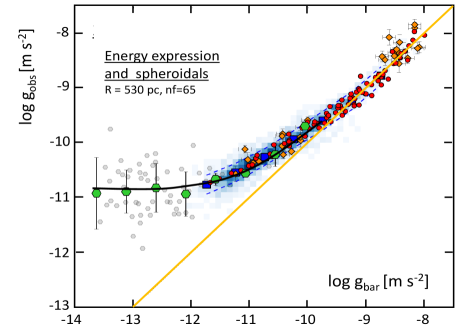
Figure 3: The same as Figs. 2, where the black curve represents the expression (21) for the spheroidals for their mean radius of 530 pcs, with $nf=65$. The binned observations for dSphs are the big green hexagons.

3.2 The case of the dwarf spheroidal galaxies

The dSphs are the objects where the mass fraction of dark matter is found to be the highest (Sancisi, 2004). The average effective radius of dwarf spheroidals is 530 pcs. Their mean representation in the $\log g_{\mathrm{obs}}$ vs. $\log g_{\mathrm{bar}}$ plot defines an horizontal asymptotic line, as suggested by Lelli et al. (2017). This asymptotic line is located at $\log g_{\mathrm{obs}}$ between -10.9 and -10.8. There are only 6 dSphs with $\log g_{\mathrm{bar}}>-11.50$. Their mean effective radius is 539 pcs, about the same as the global average and thus they may be described by the same parameters.

Let us now apply expression (21) to the sample of dSphs. We find that for the mean observed radius $R=530$ pcs, a value $nf=65$ well reproduces the observed mean distribution of the dwarf spheroidal galaxies. This distribution corresponds to a predicted asymptotic line at $\log g_{\mathrm{obs}}=-10.84$ for the lowest baryonic gravities, as illustrated by the black line in Fig. 3. The above value of $n$ should correspond to the number of equivalent tours made by a galaxy at the corresponding $g_{\mathrm{obs}}$ during its lifetime $\tau$. This number should be of the order of $n\,=\,\frac{\tau}{2\pi}\,\left(\frac{g_{\mathrm{obs}}}{R}\right)^{1/2}.$ For an age $\tau$ equal to the age of the Universe of 13.8 Gyr (Frieman et al., 2008), we get $n=65.2$. The real age may be 5 or 10% smaller, if we account for the formation time. On the whole, we see that these values are consistent.

Equation (21) describes why the dark matter, supposed to be responsible for the deviations in the plot, is found to be relatively more abundant in low gravity regions and in particular in the dwarf spheroidals. The deviations from the 1:1 line negatively depend on the ratio $(\frac{R}{g_{\mathrm{obs}}})^{\frac{1}{2}}$. Over the whole sample, the mean $g_{\mathrm{obs}}$ varies by a factor $10^{3}$, while the mean half light radii cover a smaller range from 0.5 kpc to about 15 kpc. Thus, the variations of gravities largely dominate over the variations of radii in Equation (21). Thus, despite their small radii, the dwarf spheroidals have the largest term $(\frac{R}{g_{\mathrm{obs}}})^{\frac{1}{2}}$.

The scale invariant developments well account for the fact that the dynamical gravities of the dSphs are much higher than the baryonic gravities without calling for some unknown matter component. In addition, the convergence of the distribution of the dSphs and of ultra-faint spheroidals towards an horizontal asymptotic line in the plot $\log g_{\mathrm{obs}}$ vs. $\log g_{\mathrm{bar}}$ is well reproduced. The segment of curve corresponding to the slightly higher radii and gravities for dSphs with $\log g_{\mathrm{bar}}>-11.50$ is also in agreement with observations.

3.3 The late type-galaxies (LTGs)

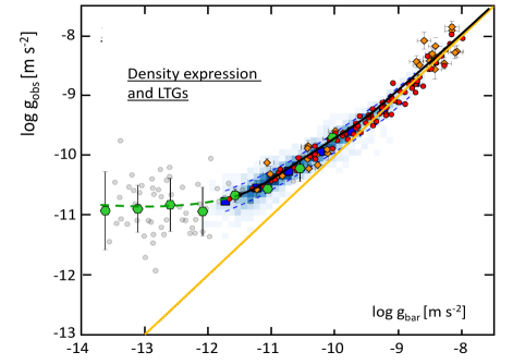
Figure 4: The same as Figs. 2 with the results of the scale invariant models. The black curve corresponds to Equation (26) applied to LTGs, with an adjustment made by continuity with the spheroidals at $\log g_{\mathrm{bar}}=-11.50$. The green broken line represents the extension for spheroidals as shown in Fig. 3.

As mentioned above, along the sequence of LTGs in the plot $\log g_{\mathrm{obs}}$ vs. $\log g_{\mathrm{bar}}$, there is a very large variety of velocities and radii. As an example, an observation for a velocity of 240 km/s at a galactocentric distance $R=60$ kpc has the same value of $g_{\mathrm{obs}}$ as for a velocity of 31 km/s at a distance of 1 kpc. One cannot associate a given radius to some value of $g_{\mathrm{obs}}$ in the plot for LTGs, contrarily to the case of dSphs. The consequence is that expression (21) is not appropriate to analyse the RAR plot of LTGs.

For these, we rather apply the expression of the deviations from the 1:1 line given by Equation (26). As a reference point to perform the adjustment of Equations (21) and (26), we consider the value $\log g_{\mathrm{bar}}=-11.5$, where the transition from LTGs to spheroidal galaxies occurs. There, Equation (21) gives a value $\log g_{\mathrm{obs}}=-10.695$ (Fig. 3). For a radius of 530 pcs, this corresponds to a velocity of 18.7 km/s. This fix the reference for the application of expression (26). (A few spiral galaxies show observations with about these values of $R$ and velocity, in particular NGC 3741, also DD0168, NGC 2455, NCG04278, UGC07524). The above value of $\log g_{\mathrm{obs}}$ implies a ratio $\left(\frac{g_{\mathrm{obs}}}{g_{\mathrm{bar}}}\right)=6.412$ at $\log g_{\mathrm{bar}}=-11.50$. Now, for other values of $\log g_{\mathrm{bar}}$ (say point 2 in Equation (26)), the ratios $g_{\mathrm{obs}}/g_{\mathrm{bar}}$ can be determined. For $\log g_{\mathrm{bar}}=-11,-10,-9,-8,-7$, one obtains $\log g_{\mathrm{obs}}=-10.29,-9.64,-8.85,-7.95,-6.98$ respectively.

Fig. 4 compares these predicted values with the observations of the radial acceleration relation for LTGs and ETGs. The agreement appears satisfactory, with a continuous evolution of the slope obtained for spheroidal galaxies. On the whole, we conclude that Equations (21) and (26), in their respective domains of application, reproduce the main features of the acceleration relation.

4 Discussion

Several observed properties of galaxies are direct consequences of the acceleration relation and are thus also consistent with the predictions of the scale invariant theory. However, this is also the case for other theories, as discussed in the introduction. Here, we briefly discuss these points and examine some way to distinguish between the various theories.

4.1 The Tully-Fisher, Faber-Jackson relations and other properties

The original Tully-Fisher relation (Tully and Fisher, 1977) relates the luminosity of spiral galaxies to the velocity in the flat part of the rotation curve. Further works by McGaugh et al. (2000) demonstrate that there is also a well defined relation between the rotation velocity $V$ in the flat part of the rotation curve and the baryonic mass $M_{\mathrm{bar}}$ of the form $M_{\mathrm{bar}}\sim V^{4}$, this relation is the so-called BTFR. As pointed out by Lelli et al. (2017), the BTFR directly results from the fact that over a part the observed acceleration relation does not follow the 1:1 line, but rather behaves more or less like $g_{\mathrm{obs}}\sim g^{1/2}_{\mathrm{bar}}$. This implies that $V^{2}\sim M^{1/2}_{\mathrm{bar}}$, which gives a behavior of the baryonic mass with about $V^{4}$. From Fig. 4, we see that the observed points of LTGs, as well as the scale-invariant relation, follow a relation $g_{\mathrm{obs}}\sim g^{\alpha}_{\mathrm{bar}}$ with $\alpha\approx 1/2$ for LTGs below $\log g_{\mathrm{bar}}<-10$. For this limited range, the above scaling of the velocity with mass is reproduced. For higher gravities, $\alpha$ increases to finally reach a value of 1 at about $\log g_{\mathrm{bar}}=-8$, leading to different slopes of the BTFR relation. These different regimes of the BTFR specifically depend on the mass–radius relation of galaxies and their detailed study is beyond the scope of the present work.

The same kind of remarks applies to the Faber-Jackson relation (Faber and Jackson, 1976), which relates the luminosity (or the stellar mass) of the elliptical galaxies to their velocity dispersion $\sigma$. As shown by Lelli et al. (2017), the facts that 1) the velocity dispersion and the rotation velocities of rotating ellipticals are linearly related, and 2) that the rotating ETGs follow the same $M_{\mathrm{bar}}\sim V^{4}$ relation as the LTGs (den Heijer et al., 2015) lead to a relation of the form $M_{\mathrm{bar}}\sim\sigma^{4}$. Also, there is a close correspondence between features in the luminosity profiles and in the rotation curves of galaxies. As quoted by Lelli et al. (2017), this property is known as ”the Renzo rule” following Sancisi (2004), who emphasizes that ”for any feature in the luminosity profile there is a corresponding feature in the rotation curve, and vice versa”. These various properties are related to the acceleration relation and consequently to its possible explanation, whatever it is.

4.2 The various interpretations of the RAR and the possibility to distinguish them

In Figs. 1 to 4, the vertical distance of the observed points above the yellow 1:1 line expresses the ratio of the dynamical (or total) masses $M_{\mathrm{dyn}}$ to the baryonic masses $M_{\mathrm{bar}}$. One has thus the correspondence $M_{\mathrm{dyn}}/M_{\mathrm{bar}}\approx g_{\mathrm{obs}}/g_{\mathrm{bar}}$ (Lelli et al., 2017). Interpreting the deviations as due to dark matter with mass $M_{\mathrm{DM}}=M_{\mathrm{dyn}}-M_{\mathrm{bar}}$, one has

$$M_{\mathrm{DM}}\,\approx\,\left(\frac{g_{\mathrm{obs}}}{g_{\mathrm{bar}}}-1\right)\,M_{\mathrm{bar}}\,.$$ (27)

For LTGs and ETGs, the ratio of dark to baryonic matter may reach a factor of 10, while for dwarf spheroidals it ranges from ten to about 400, with extreme values up to 1000. A large variety of particles, known and unknown, has been proposed since more than 30 years to account for the dark matter, see recent reviews by Bertone and Hooper (2017); de Swart et al. (2017). Several authors have proposed explanations in the framework of the $\Lambda$CDM model of galaxy formation, e.g. Navarro et al. (2017). Li et al. (2018) have also found an agreement of the RAR with the MOND theory (Milgrom, 1983, 2009). Indeed, this is not surprising since the MOND theory has been initially tailored for explaining the flat rotation curve of galaxies. Li et al. (2018) also point out that the properties of the RAR remain an open issue for $\Lambda$CDM models of galaxy formation. As seen above, the scale invariant theory gives one more interpretation of the RAR, including for the dSphs, often ignored in other interpretations.

Now, we have to see whether some predictions of the theories could permit the identification of the right one, since among the three different kinds, at least two must not apply. A signature of the scale invariant theory resides in the cumulative effects in time. This is well illustrated in the integration over the time of the modified Newton’s equation (10) performed in Section 2.3. In this respect, we note that this cumulative effect is able to account for the increase with age of the the ”vertical” velocity dispersion of stars in the Milky Way. If it is further confirmed that high redshift galaxies do not have flat rotation curves (Wuyts et al., 2016; Genzel et al., 2017; Lang et al., 2017), this may indicate that both the vertical and horizontal supports are growing with time. At present, there is no proof of that and further studies are needed.

5 Conclusions

The study of the gauging condition in Sect. 2.1 confirms the relation found earlier between the cosmological constant $\Lambda_{\mathrm{E}}$ and the scale factor $\lambda(t)$. An energy relation is obtained which well described the RAR of the dwarf spheroidal galaxies, for mean values of their radius and $\log g_{\mathrm{obs}}$. The asymptotic limit found by Lelli et al. (2017) is also confirmed. For spiral galaxies (LTGs), the relation between between the local gravity and internal density leads to an expression of the deviation of the 1:1 line in the $\log g_{\mathrm{obs}}$ vs. $\log g_{\mathrm{bar}}$ plot which agrees with the observations.

The scale invariant theory allows one to understand why the supposed dark matter is found concentrated, with large excesses, in regions of lower gravities. In this context, there is no need of dark matter to account for the observed acceleration relation. This is in agreement with previous results (Maeder, 2017c) on the missing masses of clusters of galaxies, on the rotation velocities of galaxies and on the ”vertical” velocity dispersion of stars in the Milky way. These positive results encourage further exploration.

I express my best thanks to D. Gachet for his support and to V. Gueorguiev for his support and useful comments.

References

- Bertone and Hooper (2017) Bertone, G., Hooper, D. 2017, Dark-matter history, CERN Courier, 57, vol. 4, 27
- Bond (1990) Bondi, H. 1990, in Modern Cosmology in Retrospect, Eds. Bertotti, B., Balbinot, R., & Bergia, S., Cambridge Univ. Press., 426 pp.
- Bouvier and Maeder (1978) Bouvier, P., Maeder, A. 1978, Astrophys. Space Science, 54, 497
- Canuto et al. (1977) Canuto, V., Adams, P. J., Hsieh, S.-H., & Tsiang, E. 1977, Phys. Rev. D, 16, 1643
- Carroll et al. (1992) Carroll, S. M., Press, W. H., & Turner, E. L. 1992, ARA&A, 30, 499
- den Heijer et al. (2015) den Heijer, M., Oosterloo, T.A., Serra, P. et al. 205, Astron. Astrophys. 581, A98
- Desmond (2017) Desmond, H. 2017, MNRAS, 464, 4160
- de Swart et al. (2017) de Swart, J.G., Bertone, G., Hooper, D. 2017, Nature Astronomy, 1,
- Dirac (1973) Dirac, P. A. M. 1973, Proceedings of the Royal Society of London Series A, 333, 403
- Di Cintio and Lelli (2016) Di Cintio, A., Lelli, F. 2017, MNRAS, 456, L127
- Eddington (1923) Eddington, A. S. 1923, The mathematical theory of relativity, Chelsea Publ. Co. New York, 270 p.
- Faber and Jackson (1976) Faber, S. M. and Jackson, R. E. 1976, ApJ, 204, 668
- Frieman et al. (2008) Frieman, J. A., Turner, M. S., & Huterer, D. 2008, ARA&A, 46, 38
- Genzel et al. (2017) Genzel, R., Schreiber, N.M., Forster Schreiber, N.M., Ubler, H. 2017, Nature, 543, 397
- Keller and Wadsley (2017) Keller, B.W., Wadsley, J.W. 2017, ApJ, 835, L17
- Lang et al. (2017) Lang, P., Forster Schreiber, N.M., Genzel, R. 2017, ApJ, 840, 92L
- Lelli et al. (2016) Lelli, F., McGaugh, S.S., Schombert, J.M., 2016, AJ, 152, 157
- Lelli et al. (2017) Lelli, F., McGaugh, S.S., Schombert, J.M., Pawlowski, M.S., 2017, ApJ, 836, 152
- Li et al. (2018) Li, P., Lelli, F., McGaugh, S. et al. 2018, arXiv:1803.00022
- Ludlow et al. (2017) Ludlow, A.D., Benitez-Lambay, A. Schaller, M. e al. 2017, PhRvL. 118p1103
- Maeder (2017a) Maeder, A. 2017a, ApJ, 834, 194
- Maeder (2017b) Maeder, A. 2017b, ApJ, 847, 65
- Maeder (2017c) Maeder, A. 2017c, ApJ, 849, 158
- Maeder and Bouvier (1979) Maeder, A., Bouvier, P. 1979, Astron. Astrophys., 73, 82
- McGaugh (2004) McGaugh, S.S. 2004, ApJ, 609, 652
- McGaugh et al. (2000) McGaugh, S.S., Schombert, J.M., Bothun, G.D. and de Blok, W. J. G. 2000, ApJ, 533, L99
- McGaugh et al. (2016) McGaugh, S.S., Lelli, F., Schombert, J.M. 2017, Phys. Rev. Letters, 117, 201101
- Milgrom (1983) Milgrom, M. 1983, ApJ, 270, 365
- Milgrom (2009) Milgrom, M. 2009, ApJ, 698, 1630
- Milgrom (2016) Milgrom, M. 2016, arXiv:1609.06642
- Navarro et al. (2017) Navarro, J.F., Benitez-Llambay, A., Fattahi, A. et al. 2017, MNRAS, 471, 1841
- Sancisi (2004) Sancisi, R. 2004, IAU Symp. 220, Dark Matter in Gakaxies, ed. S. Ryder et al., p. 233
- Santos-Santos (2016) Santos-Santos, I.M., Brook, C.B., Stinson, G. et al. 2016, MNRAS, 455, 476
- Sofue and Rubin (2001) Sofue, Y., Rubin, V. 2001, ARA&A, 39, 137
- Sohn et al. (2017) Sohn, J., Geller , M. J., Zahid, H. J. et al. 2016, ApJS, 229, 20
- Strigari et al. (2008) Strigari, L. E., Koushiappas, S. M., Bullock, J. S. 2008, ApJ, 678, 614
- Tully and Fisher (1977) Tully, R. B., Fisher, J.R. 1977, Astron. Astrophys., 54, 661
- Weyl (1923) Weyl, H. 1923, Raum, Zeit, Materie. Vorlesungen über allgemeine Relativitätstheorie. Re-edited by Springer Verlag, Berlin, 1970
- Wuyts et al. (2016) Wuyts, S., Forster Schreiber, N.M., Wisnioski, E. 2016, ApJ, 831, 149