Photon echo using imperfect X-ray pulse with phase fluctuation

Abstract

We study the impact of inter-pulse phase fluctuation in free-electron X-ray laser on the signal in the photon echo spectroscopy, which is one of the simplest non-linear spectroscopic methods. A two-pulse echo model is considered with two-level atoms as the sample. The effect of both fluctuation amplitude and correlation strength of the random phase fluctuation is studied both numerically and analytically. We show that the random phase effect only affects the amplitude of the photon echo, yet not change the recovering time. Such random phase induces the fluctuation of recovering amplitude in the photon echo signals among different measurements. We show the normal method of measuring coherence time retains by averaging across the signals in different repeats in current paper.

I Introduction

The recent development of x-ray source, especially the large facility x-ray free-electron laser(XFEL), has attracted vast amount of attentions (Ullrich et al., 2012; Geloni, 2017; Bostedt et al., 2016) towards detecting properties beyond the scope of traditional instruments. The unique features of the high brightness, short pulse duration, and frequency range of XFEL light source open new era in the scientific investigations in atomic, molecular physics and biology (Lindau, 1997; Prat et al., 2015; Bostedt et al., 2016). One potential application is the implementation of nonlinear spectroscopy (Mukamel, 2005; Schweigert and Mukamel, 2007, 2008; Mukamel et al., 2013; Healion et al., 2013; Bennett et al., 2016) to investigate the dynamics of matter in extreme conditions. The non-linear spectroscopy typically requires high degree of temporal coherence (Mukamel, 1995; Schlau-Cohen et al., 2011), i.e. inter-pulse phase stability as well as intra-pulse stability (Schlau-Cohen et al., 2011). However, pulses generated from many current facilities, may not fulfill such requirement due to its inter-pulse phase fluctuation (Yu, 1991; Wang and Yu, 1986; Bostedt et al., 2016; Lee et al., 2012; Yu et al., 2000). A direct question is how such phase fluctuation affects on the actually signal, especially on methods of extracting key parameters, e.g coherence time.

We will investigate the impact of inter-pulse phase fluctuation of x-ray pulses on photon echo, which is one of the simplest nonlinear spectroscopy methods, yet fundamental to many advanced spectroscopic methods, e.g. two-dimensional electronic spectroscopy and two-dimensional vibrational spectroscopy (Schlau-Cohen et al., 2011; Mukamel, 1995). Photon echo (Abella et al., 1966; Shvyd’ko, 2016; Scully et al., 1968) is an optical analogy to spin echo, and is designed to remove ensemble average for measuring properties of individual spins while maintaining signal amplitude by avoiding measuring individuals directly (Mukamel, 1995). Taking a simple two-level system as an example, an excitation pulse creates an initial state $\left|\psi\left(0\right)\right\rangle=\alpha\left|g\right\rangle+\beta\left|e\right\rangle$, where $\left|g\right\rangle$ and $\left|e\right\rangle$ are the ground and excited state with energies 0 and $\epsilon_{e}$ respectively. The free evolution brings the system to the state $\left|\psi\left(t\right)\right\rangle=\alpha\left|g\right\rangle+\beta\exp(-i\epsilon_{e}t)\left|e\right\rangle$. A subsequent $\pi/2$ pulse reverses the population $\left|\psi^{\prime}\left(t\right)\right\rangle=\alpha\left|e\right\rangle+\beta\exp(-i\epsilon_{e}t)\left|g\right\rangle$. The later evolution compensates the phase accumulated during the evolution of ensemble between the two pulses, namely, $\left|\psi\left(T,t\right)\right\rangle=\alpha\exp(-i\epsilon_{e}T)\left|e\right\rangle+\beta\exp(-i\epsilon_{e}t)\left|g\right\rangle.$ At a revival time $T=t$ , the impact of disorder (inhomogenerity) over the signal is essentially removed. However, it is usually not easy to achieve the $\pi/2$ pulse due to the weak pulse intensity in the optical region. One solution is to use non-colinear incident pulses in order to separate the echo signal from other signal via phase matching method, which is frequently adopted in non-linear spectroscopy studies (Mukamel, 1995).

This paper is organized as follows. In Sec. II, we show the general model of measuring the signal of two-pulse photon echo on the ensemble of two-level atoms with imperfect x-ray pulse. In Sec. III, we show the analytical result of photon echo under the influence of phase instability along with exact numerical results.

II Photon echo with imperfect X-ray pulse

In the current paper, we consider an ensemble of two-level atoms with the ground state $\left|g\right\rangle$ and the excited state $\left|e\right\rangle$. The free Hamiltonian for the two-level atom is

$$H_{0}=\epsilon_{e}\left|e\right\rangle\left\langle e\right|,$$ (1)

where we have set the energy of the ground state as $\epsilon_{g}=0$. The energy levels here are inner-shell electronic states (Mukamel et al., 2013), accessible with the frequency of XFEL. The interaction Hamiltonian between pulses and the atom is given by the dipole interaction $H_{I}=-\vec{\mu}\cdot\vec{E}\left(t\right),$ where $\vec{\mu}$ is the transition dipole and $\vec{E}\left(t\right)$ is the electric field of the incident X-ray pulse. Under the rotation wave approximation, the interaction Hamiltonian for a pulse with central frequency $\text{$\nu$}_{0}$ and wave vector $\vec{k}$ is simplified as

$$H_{I}=-\Omega\left(t\right)e^{-i\nu_{0}t-i\phi\left(t\right)+i\vec{k}\cdot\vec{r}}\left|e\right\rangle\left\langle g\right|+h.c.,$$ (2)

where $\phi\left(t\right)$ characterizes the random phase of the X-ray pulse, $\vec{r}$ is the spatial location of the atom, and $\Omega(t)$ is the Rabi frequency. We simplify the model with the square pulse approximation: the strength of the pulse is a constant $\Omega$ in the duration for the pulse and diminishes when the pulse ends.

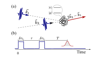
Figure 1: The model and pulse sequence. (a) The two incident pulses are directed to the sample in a non-colinear geometry along two directions $\vec{k}_{1}$ and $\vec{k}_{2}$. The emission of the two-pulse photon echo is along the direction $2\vec{k}_{2}-\vec{k}_{1}$. The sample is an ensemble of two-level atoms with the ground state $\left|g\right\rangle$ and excited state $\left|e\right\rangle$. (b) The blue line shows the two pulses, and the red line show the signal. The duration of the two pulse are $\delta\tau_{1}$ and $\delta\tau_{2}$, and the delay time is $\tau$. And the measurement of the echo signal acts at $T$ time after the end of the second pulse.

Here, we consider the two-pulse photon echo, and the two pulses are set to be resonated to the atom $\nu_{0}=\epsilon_{e}.$ The first pulse interacts with the atoms with the duration $\delta\tau_{1}$, while the second pulse interacts with the atoms with the duration time $\delta\tau_{2}$ after delay time $\tau$ of the end of the first pulse. The evolution matrices for each pulse are $U_{i}(\vec{k}_{i},\delta\tau_{i})\,(i=1,2)$, and the free evolution of the atom is $U_{0}(t_{f},t_{i})=U_{0}(t_{f}-t_{i})=\exp[-iH_{0}(t_{f}-t_{i})]$, where $t_{i}(t_{f})$ is the initial (final) time of the free evolution. The final wave function of the atom at delay time $T$ is obtained as

$$\left|\psi\left(T,\tau\right)\right\rangle=U_{0}\left(T\right)U_{2}(\vec{k}_{2},\delta\tau_{2})U_{0}\left(\tau\right)U_{1}(\vec{k}_{1},\delta\tau_{1})\left|\psi_{0}\right\rangle,$$ (3)

where the initial state $\left|\psi_{0}\right\rangle$ is usually considered as the ground state $\left|\psi_{0}\right\rangle=\left|g\right\rangle$. To derive the evolution matrices $U_{i}(k_{i},\delta\tau_{i})$ for each pulse, we rewrite the Hamiltonian in the interacting picture as

$$\hat{H}_{I}(t)=-\left(\begin{array}[]{cc}0&\hbar\Omega_{a}e^{i\phi(t)-i\vec{k}\cdot\vec{r}}\\ \hbar\Omega_{a}e^{-i\phi(t)+i\vec{k}\cdot\vec{r}}&0\end{array}\right).$$ (4)

The time dependence of Eq. (4) only comes from the random phase factor $\phi\left(t\right)$. With the following definitions

$$H_{1}\left(\vec{k}\right)=\left(\begin{array}[]{cc}0&\hbar\Omega e^{-i\vec{k}\cdot\vec{r}}\\ \hbar\Omega e^{i\vec{k}\cdot\vec{r}}&0\end{array}\right),$$ (5)

$$H_{2}\left(\vec{k}\right)=\left(\begin{array}[]{cc}0&-i\hbar\Omega e^{-i\vec{k}\cdot\vec{r}}\\ i\hbar\Omega e^{i\vec{k}\cdot\vec{r}}&0\end{array}\right),$$ (6)

$$H_{3}\left(\vec{k}\right)=\left(\begin{array}[]{cc}\hbar\Omega&0\\ 0&-\hbar\Omega\end{array}\right),$$ (7)

$\hat{H}_{I}(t)$ is rewritten in a compact form

$$\hat{H}_{I}(t)=-\cos\left[\phi(t)\right]H_{1}+\sin\left[\phi(t)\right]H_{2}.$$ (8)

The three operators $H_{l}\,(l=1,2,3)$ satisfy the commutation relation of angular momentum operators $[H_{i}(\vec{k}),H_{j}(\vec{k})]=2i\hbar\sum_{l=1}^{3}\Omega H_{l}(\vec{k})\epsilon_{ijl}.$ Following the Wei-Norman algebra method (Wei and Norman, 1963; Sun and Xiao, 1991), the evolution matrix for a pulse is written as

$$\hat{U}_{\vec{k},\phi}\left(t,0\right)=e^{-i\chi_{3}(t)H_{3}}e^{-i\chi_{2}(t)H_{2}}e^{-i\chi_{1}(t)H_{1}},$$ (9)

where $\vec{k}$ is the wave vector and $\phi$ is a certain realization of the random phase. With the commutation relation of $H_{l}\,(l=1,2,3)$, we have derived the differential equations for the time-dependent parameters $\{\chi_{l}\left(t\right)\},\,(l=1,2,3)$ in Appendix A

$$\left\{\begin{array}[]{l}\dot{\chi}_{3}=-\cos(\phi+2\chi_{3}\Omega)\tan 2\chi_{2}\Omega\\ \dot{\chi}_{2}=\sin(\phi+2\chi_{3}\Omega)\\ \dot{\chi}_{1}=-\cos(\phi+2\chi_{3}\Omega)\sec 2\chi_{2}\Omega.\end{array}\right.$$ (10)

The initial condition is $\chi_{l}\left(0\right)=0,\;l=1,2,3$. The non-linear time-dependent differential equations (10) are accessible to be solved numerically with a given $\phi(t)$.

Next, we change the evolution matrices derived by Eq.(9) from the interacting picture to Schrodinger picture, which is linked by a free evolution $U_{1}(\vec{k}_{1},\delta\tau_{1})=U_{0}\left(\delta\tau_{1}\right)\hat{U}_{\vec{k}_{1},\phi_{1}}\left(\delta\tau_{1},0\right)$ and $U_{2}(\vec{k}_{2},\delta\tau_{2})=U_{0}\left(\delta\tau_{2}\right)\hat{U}_{\vec{k_{2}},\phi_{2}}\left(\delta\tau_{2},0\right).$ $U_{0}(\delta\tau_{i})$ is absorbed to the free evolution part or neglected when $\delta\tau_{i}$ is small compared to the interval time $\tau$ and the measurement time $T$. Combined with Eq. (3), the echo term is derived by sorting terms with the phase factor matching $\exp[i(2\vec{k}_{2}-\vec{k}_{1})\cdot\vec{r}]$ as follows,

$$\begin{array}[]{l}\left\langle\psi\left(T,\tau\right)\right|\mu_{t}\left|\psi\left(T,\tau\right)\right\rangle\\ \sim i\mu^{*}e^{-i\left(T-\tau\right)\epsilon_{e}}e^{i(2\vec{k}_{2}-\vec{k}_{1})\cdot\vec{r}}\\ \times\frac{e^{2i\Omega\left(\zeta_{3}-\chi_{3}\right)}}{8}\left[\sin((\zeta_{2}+\zeta_{1})\Omega)+i\sin((\zeta_{2}-\zeta_{1})\Omega)\right]{}^{2}\\ \times\left[\sin(2(\chi_{2}-\chi_{1})\Omega)+2i\sin(2\chi_{1}\Omega)+\sin(2(\chi_{2}+\chi_{1})\Omega)\right].\end{array}$$ (11)

For the ensemble of atoms, their energy $\epsilon_{e}$ between the ground state and the excited state has fluctuations, assumed as Gaussian distribution with mean value $\epsilon_{0}$ and variance $\sigma_{0}^{2}$ with the following form,

$$p\left(\epsilon_{e}\right)=\frac{1}{\sqrt{2\pi}\sigma_{0}}\exp\left[-\frac{(\epsilon_{e}-\epsilon_{0})^{2}}{2\sigma_{0}^{2}}\right].$$ (12)

The summation over transition energies of different molecules contributes a Gaussian decay with $(T-\tau)$, namely,

$$\sum_{\epsilon_{e}}e^{-i\left(T-\tau\right)\epsilon_{e}}\rightarrow e^{-\frac{1}{2}\sigma_{0}^{2}(T-\tau)^{2}-i\left(T-\tau\right)\epsilon_{0}}.$$ (13)

At the revival time $T=\tau$, the average over different molecules vanishes so that decoherence time can be directly detected. The amplitude $\mathcal{A}$ of the photon echo signal is the square of the absolute value of Eq. (11)

$$\begin{array}[]{l}\mathcal{A}=\frac{\left|\mu\right|^{2}e^{-\sigma_{0}^{2}(T-\tau)^{2}}}{64}\left[\sin^{2}((\zeta_{2}+\zeta_{1})\Omega)+\sin^{2}(\zeta_{2}-\zeta_{1})\Omega\right]^{2}\\ \left[\left(\sin(2(\chi_{2}-\chi_{1})\Omega)+\sin(2(\chi_{2}+\chi_{1})\Omega)\right)^{2}+4\sin^{2}(2\chi_{1}\Omega)\right]\end{array}$$ (14)

For the ideal case with no random phase ($\phi\left(t\right)=\mathrm{constant}$), we obtain the amplitude

$$\mathcal{A}_{\mathrm{ideal}}=\frac{\left|\mu\right|^{2}e^{-\sigma_{0}^{2}(T-\tau)^{2}}}{4}\sin^{4}(\Omega\delta\tau_{2})\sin^{2}(2\Omega\delta\tau_{1}).$$ (15)

with $\chi_{2}^{(0)}=\chi_{3}^{(0)}=\zeta_{2}^{(0)}=\zeta_{3}^{(0)}=0,\chi_{1}^{(0)}=-\delta\tau_{1},\zeta_{1}^{(0)}=-\delta\tau_{2}$. It is clear that the random phase only affects the amplitude of the photon echo. A factor $\mathcal{F}$ is defined to represent the value of the amplitude

$$\mathcal{F} =\{\sin^{2}[(\zeta_{2}+\zeta_{1})\Omega]+\sin^{2}[(\zeta_{2}-\zeta_{1})\Omega]\}^{2}$$

$$\times\left[[\sin[2(\chi_{2}-\chi_{1})\Omega]+\sin[2(\chi_{2}+\chi_{1})\Omega]]^{2}+4\sin(2\chi_{1}\Omega)^{2}\right].$$ (16)

In the following discussion, we consider the two pulses is the same except different direction, namely, $\delta\tau_{1}=\delta\tau_{2}=\delta\tau$, and $\chi_{i}=\zeta_{i}$ $\left(i=1,2,3\right).$ For the case without phase fluctuation ($\phi\left(t\right)=\mathrm{constant}$), the factor $\mathcal{F}$ is simply

$$\mathcal{F}_{\mathrm{ideal}}=16\sin^{4}(\Omega\delta\tau)\sin^{2}\left(2\Omega\delta\tau\right).$$ (17)

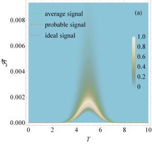
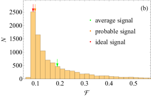
Figure 2: The photon echo signal and the distribution of strength factor $\mathcal{F}$. The parameters are chosen as $\tau=5$, $\sigma_{0}=1$,$\Omega=1$, $\delta\tau=4.75$ ,$\gamma=1/4.587$, $\Phi=0.08$. (a) the distribution of the signal at time $T$. The color shows the probability at given time $T$ with the amplitude $\mathcal{A}$. The green curve and the orange curve shows the average signal and the most probable signal respectively, while the red curve shows the ideal echo signal without any phase randomness. (b) the distribution of the strength factor $\mathcal{F}$ with 10000 repeats for echo signal at $T=\tau$. The arrows show the average, most probable, and ideal signal with the same color scheme as in subfigure (a).

In Fig 2(a), we show the distribution of the signal intensity $\mathcal{A}$ as a function of $T$. The random phase elicits fluctuation to the signal and enlarges the average value. In the simulation, we generate the random function $\phi(t)$ with the Ornstein-Uhlenbeck process. The average of $\phi(t)$ is zero $\left\langle\phi\left(t\right)\right\rangle=0$, and its two-point correlation function satisfies

$$\left\langle\phi\left(t_{1}\right)\phi\left(t_{2}\right)\right\rangle=\Phi^{2}e^{-\gamma\left|t_{1}-t_{2}\right|},$$ (18)

where $\Phi$ is the fluctuation amplitude of the random phase and $\gamma$ is the correlation strength. The amplitude of signal is evaluated via Eq. (11) with $\chi_{i}$ and $\zeta_{i}$, which is numerically solved the differential equation (10). The statistics is calculated with 10000 repeats of the current process by generating different random function $\phi(t)$. In the simulation, we have chosen parameters as follows, $\tau=5,\>\sigma=1,\>\Omega=1,\>\delta\tau=4.75,\>\gamma=1/4.587,$ and $\Phi=0.08$. In Fig. 2(a), we show the average signal with green dashed line, the most probable signal with orange dashed line, and the signal without random phase with red dotted line. We further show the randomness of the factor $\mathcal{F}$ in Fig 2(b), whose distribution $p(\mathcal{F})$ is not Gaussian. The mean value of $\mathcal{F}$ is larger than the most probable case and the ideal case (the case without random phase). It is clear that the random phase induces fluctuation on the strength of the signal of the photon echo.

With the observation of the randomness of the echo amplitude, it is meaningful to calculate the average signal with different repeats. Here, we try to derive perturbation results for the average amplitude $\langle\mathcal{A}\rangle$ with random phase. We consider the random phase is small and apply the approximation $\cos\phi(t)\approx 1,\>\sin\phi(t)\approx\phi(t)$ to obtain the linear differential equation of Eq.(10) for $\chi_{2}$ and $\chi_{3}$ as follows. The differential equation for $\chi_{1}$ is kept for second order to obtain the signal amplitude to the second order

$$\left\{\begin{array}[]{l}\dot{\chi}_{3}=-2\Omega\chi_{2}\\ \dot{\chi}_{2}=\phi+2\Omega\chi_{3}\\ \dot{\chi}_{1}=-1+\frac{1}{2}\left(\phi+2\chi_{3}\Omega\right)^{2}-\frac{1}{2}\left(2\chi_{2}\Omega\right)^{2}.\end{array}\right.$$ (19)

Now, the current equation (19) has an integral solution

$$\begin{array}[]{c}\chi_{3}\left(t\right)=-\int_{0}^{t}\sin 2\Omega\left(t-t_{1}\right)\phi\left(t_{1}\right)dt_{1}\\ \chi_{2}\left(t\right)=\int_{0}^{t}\cos 2\Omega\left(t-t_{1}\right)\phi\left(t_{1}\right)dt_{1}\\ \chi_{1}\left(t\right)=-t+\int_{0}^{t}\frac{1}{2}\phi^{2}+2\Omega\chi_{3}\phi+2\Omega^{2}\chi_{3}^{2}-2\Omega^{2}\chi_{2}^{2}dt_{1}.\end{array}$$ (20)

For small random phase $\phi(t)$, we expand the factors $\chi_{i},\>i=1,2,3$ to their first order $\chi_{i}=\chi_{i}^{(0)}+\chi_{i}^{(1)}$ , where $\chi_{i}^{(0)}$ is the average value, i.e., $\chi_{1}^{(0)}=0,\>\chi_{2}^{(0)}=0,\,\chi_{3}^{(0)}=-\delta\tau$ and $\chi_{i}^{(1)}$ gives the fluctuation due to the random phase. We obtain the explicit form of the factor $\mathcal{F}$ under the perturbation formalism

$$\begin{array}[]{l}\begin{array}[]{l}\mathcal{F}=\mathcal{F}_{\mathrm{ideal}}-128\chi_{1}^{(1)}\Omega\sin^{5}(\delta\tau\Omega)(2\cos(\delta\tau\Omega)+\cos(3\delta\tau\Omega))\end{array}\\ +64\left(\chi_{2}^{(1)}\right)^{2}\Omega^{2}\sin^{4}(\delta\tau\Omega)\cos(2\delta\tau\Omega)(2\cos(2\delta\tau\Omega)+1).\end{array}$$ (21)

Eq. (21) contains $\chi_{2}^{(1)}$ to the second order and $\chi_{1}^{(1)}$ to the first order. It is verified numerically that $\chi_{1}^{(1)}$ is as the same order as $(\chi_{2}^{(1)})^{2}$ in Appendix B. And they are both the lowest order contributing to $\mathcal{F}$.

The factor $\mathcal{F}$ is a random variable due to the random phase $\phi(t)$. We derive the average value $\left\langle(\chi_{2}^{(1)})^{2}\right\rangle$ and $\left\langle\chi_{1}^{(1)}\right\rangle$ by the two-point correlation function. The detailed calculation is attached in the Appendix B. The analytical result for the mean value of $\mathcal{F}$ becomes

$$\begin{array}[]{l}\mathcal{\left\langle\mathcal{F}\right\rangle}=\mathcal{F}_{\mathrm{ideal}}\\ +64\Omega^{2}\sin^{4}(\delta\tau\Omega)\cos(2\delta\tau\Omega)(2\cos(2\delta\tau\Omega)+1)\left\langle(\chi_{2}^{(1)})^{2}\right\rangle\\ -128\Omega\sin^{5}(\delta\tau\Omega)(2\cos(\delta\tau\Omega)+\cos(3\delta\tau\Omega))\left\langle\chi_{1}^{(1)}\right\rangle.\end{array}$$ (22)

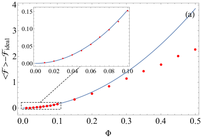
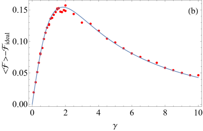
Figure 3: The relation between $\left\langle\mathcal{F}\right\rangle-\mathcal{F}_{\mathrm{ideal}}$ and the fluctuation amplitude $\Phi$ and the correlation strength $\gamma$ . The parameters are chosen as $\Omega=1$, $\delta\tau=4.75$ ,$\gamma=1/4.587$ for the figure 3 (a), (c), $\Phi=0.05$ for figure 3 (b). The red points shows the numerical calculation and the solid curve shows the analytical result.

In Fig 3 (a), we plot the average signal $\left\langle\mathcal{F}\right\rangle-\mathcal{F}_{\mathrm{ideal}}$ as a function of the fluctuation amplitude $\Phi$ with the correlation strength $\gamma$ fixed. In the figure, red dots show the exact result by numerical calculation, and lines represent the analytical result in Eq. (22). For small fluctuation amplitude $\Phi$, the analytical result matches numerical calculation well, as illustrated in subset of Fig 3 (a). However, the analytical result deviates from exact numerical result for large $\Phi$, e.g. $\Phi>0.3$. In Fig 3 (b), we plot the average signal $\left\langle\mathcal{F}\right\rangle-\mathcal{F}_{\mathrm{ideal}}$ as a function of the correlation strength $\gamma$ with the fluctuation amplitude $\Phi$ fixed. The analytical result matches numerical calculation well whether for large or small $\gamma$.

In above discussion, we have shown the random phase effect on the signal amplitude of an ensemble of two-level atoms without any decoherence. The key function of photon echo is to measure the decoherence time $\tau_{c}$. In open systems, the environment induces a decoherence to the atoms, which contributes to the decreasing of the non-diagonal term $\rho_{eg}(t)=\exp[-i\epsilon_{e}t-t/\tau_{c}]$. With the decoherence effect, the signal derived in Eq. (16) becomes

$$\begin{array}[]{l}\mathcal{A}_{\mathrm{open}}=\frac{\left|\mu\right|^{2}e^{-\sigma_{0}^{2}(T-\tau)^{2}-\left(T+\tau\right)/\tau_{c}}}{64}\mathcal{F}.\end{array}$$ (23)

At the revival time $T=\tau$, the average signal is

$$\langle\mathcal{A}_{\mathrm{open}}\rangle=\left|\mu\right|^{2}\exp(-2\tau/\tau_{c})\langle\mathcal{F}\rangle.$$ (24)

With fixed $\delta\tau$ and given random phase, the average for the factor $\mathcal{F}$ is invariant. To measure the coherence time $\tau_{c}$, we still follow the normal way of changing the delay time $\tau$ and obtain the signal amplitude at $T=\tau$. By taking average over different repeats, the coherence time is recovered via Eq. (24).

Currently, the experimental setup of x-ray photon echo is achievable with the split-delay approach (Gutt et al., 2008; Roseker et al., 2011), where the x-ray pulse is split by a silicon beam splitter(Roseker et al., 2011). The change to the setup in Ref (Gutt et al., 2008) is to direct the splitted two pulses to the sample along two directions. With the split-delay approach, the phase difference between pulses is fixed with delay time. And the phase fluctuation of each pulses is theoretically considered in the current paper.

III Conclussion

We have theoretically calculated the impact of phase randomness on the photon echo experiment, which is fundamental to many other non-linear spectroscopy, such as two-dimensional spectroscopy. We found that the phase randomness will induce fluctuation in the photon echo signal, yet not affect the rephasing time. By averaging the signal from different repeats, the normal way of photon echo is still effective for measuring the decoherence time.

Appendix A Wei Norman Method

In this appendix, we show the detailed derivation of the differential equation (10). The derivation is based on the Wei-Norman algebra method(Sun and Xiao, 1991; Wei and Norman, 1963). The differential of Eq. (9) is calculated

$$\begin{array}[]{l}\frac{d}{dt}U_{p,\phi}(t,0)=-i\dot{\chi}_{3}H_{3}U_{p,\phi}(t,0)\\ \qquad-i\dot{\chi}_{2}e^{-i\chi_{3}H_{3}}H_{2}e^{-i\chi_{2}H_{2}}e^{-i\chi_{1}H_{1}}\\ \qquad-i\dot{\chi}_{1}U_{p,\phi}(t,0)H_{1}\end{array}$$ (25)

With the commutations

$$e^{-i\chi_{3}H_{3}}H_{2}e^{i\chi_{3}H_{3}}=H_{2}\cos 2\Omega\chi_{3}-H_{1}\sin 2\Omega\chi_{3},$$ (26)

$$\begin{array}[]{l}e^{-i\chi_{3}H_{3}}e^{-i\chi_{2}H_{2}}H_{1}e^{i\chi_{2}H_{2}}e^{i\chi_{3}H_{3}}=-H_{3}\sin 2\Omega\chi_{2}\\ \qquad+H_{2}\sin 2\Omega\chi_{3}\cos 2\Omega\chi_{2}\\ \qquad+H_{1}\cos 2\hbar\Omega\chi_{3}\cos 2\Omega\chi_{2}\end{array},$$ (27)

Eq. (25) is rewritten as

$$\begin{array}[]{l}i\frac{\partial}{\partial t}U_{p,\phi}\left(t,0\right)=[\left(\dot{\chi}_{3}-\dot{\chi}_{1}\sin 2\Omega\chi_{2}\right)H_{3}\\ +\left(\dot{\chi}_{1}\sin 2\Omega\chi_{3}\cos 2\Omega\chi_{2}+\dot{\chi}_{2}\cos 2\Omega\chi_{3}\right)H_{2}\\ +\left(\dot{\chi}_{1}\cos 2\Omega\chi_{3}\cos 2\Omega\chi_{2}-\dot{\chi}_{2}\sin 2\Omega\chi_{3}\right)H_{1}]U_{p,\phi}\left(t,0\right).\end{array}$$ (28)

The coefficients must match the Schrodinger equation (8)

$$\left(\begin{array}[]{ccc}0&-\sin 2\Omega\chi_{3}&\cos 2\Omega\chi_{3}\cos 2\Omega\chi_{2}\\ 0&\cos 2\Omega\chi_{3}&\sin 2\Omega\chi_{3}\cos 2\Omega\chi_{2}\\ 1&0&-\sin 2\Omega\chi_{2}\end{array}\right)\left(\begin{array}[]{c}\dot{\chi}_{3}\\ \dot{\chi}_{2}\\ \dot{\chi}_{1}\end{array}\right)=\left(\begin{array}[]{c}-\cos\phi\\ \sin\phi\\ 0\end{array}\right).$$ (29)

The differential equations are obtained by taking the inverse matrix

$$\left\{\begin{array}[]{l}\dot{\chi}_{3}=-\cos\phi\cos 2\chi_{3}\Omega\tan 2\chi_{2}\Omega+\sin\phi\sin 2\chi_{3}\Omega\tan 2\chi_{2}\Omega\\ \dot{\chi}_{2}=\cos 2\chi_{3}\Omega\sin\phi+\cos\phi\sin 2\chi_{3}\Omega\\ \dot{\chi}_{1}=-\cos\phi\cos 2\chi_{3}\Omega\sec 2\chi_{2}\Omega+\sin\phi\sec 2\chi_{2}\Omega\sin 2\chi_{3}\Omega\end{array}\right.$$ (30)

With further simplification we obtain Eq. (10).

Appendix B The Calculation of $\left\langle\left(\chi_{2}^{(1)}\right)^{2}\right\rangle$ and $\left\langle\chi_{1}^{(1)}\right\rangle$

Here, we give the detailed calculation for$\left\langle(\chi_{2}^{(1)})^{2}\right\rangle$ and $\left\langle\chi_{1}^{(1)}\right\rangle$. With Eq. (20), we can calculate the average value of $(\chi_{2}^{(1)})^{2}$

$$\left\langle(\chi_{2}^{(1)})^{2}\right\rangle=\int_{0}^{\delta\tau}\int_{0}^{\delta\tau}\cos 2\Omega\left(t-t_{1}\right)\cos 2\Omega\left(t-t_{2}\right)\left\langle\phi\left(t_{1}\right)\phi\left(t_{2}\right)\right\rangle dt_{2}dt_{1}.$$ (31)

The result of the integral gives

$$\left\langle(\chi_{2}^{(1)})^{2}\right\rangle=\Phi^{2}\left(\frac{\gamma\delta\tau}{\gamma^{2}+4\Omega^{2}}+\frac{2\gamma e^{-\gamma\delta\tau}\left(\gamma\cos\left(2\delta\tau\Omega\right)-2\Omega\sin\left(2\delta\tau\Omega\right)\right)}{\left(\gamma^{2}+4\Omega^{2}\right)^{2}}+\frac{\gamma\sin\left(4\delta\tau\Omega\right)-2\Omega\cos\left(4\delta\tau\Omega\right)}{4\Omega\left(\gamma^{2}+4\Omega^{2}\right)}+\frac{8\Omega^{2}-6\gamma^{2}}{4\left(\gamma^{2}+4\Omega^{2}\right)^{2}}\right).$$ (32)

It is similar to calculate the average value of $\chi_{1}^{(1)}$

$$\left\langle\chi_{1}^{(1)}\right\rangle=\left\langle\int_{0}^{\delta\tau}\left(\frac{1}{2}\phi^{2}+2\Omega\chi_{3}\phi+2\Omega^{2}\chi_{3}^{2}-2\Omega^{2}\chi_{2}^{2}\right)dt_{1}\right\rangle.$$ (33)

The result is

$$\left\langle\chi_{1}^{(1)}\right\rangle=\Phi^{2}\left(\frac{\gamma^{2}\delta\tau}{2\gamma^{2}+8\Omega^{2}}-\frac{2\gamma\Omega e^{-\gamma\delta\tau}(\gamma\sin(2\delta\tau\Omega)+2\Omega\cos(2\delta\tau\Omega))}{\left(\gamma^{2}+4\Omega^{2}\right)^{2}}+\frac{\Omega\sin(4\delta\tau\Omega)-\gamma\sin^{2}(2\delta\tau\Omega)}{2\left(\gamma^{2}+4\Omega^{2}\right)}+\frac{4\gamma\Omega^{2}}{\left(\gamma^{2}+4\Omega^{2}\right)^{2}}\right).$$ (34)

And we show the numerical calculation matches the analytical result in Figure 5, which shows that $\left\langle(\chi_{2}^{(1)})^{2}\right\rangle$ and $\left\langle\chi_{1}^{(1)}\right\rangle$ are the same order and should be kept for the perturbation.

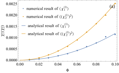
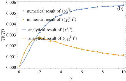
Figure 4: The numerical and analytical result of $\left\langle\chi_{1}^{(1)}\right\rangle$ and $\left\langle(\chi_{2}^{(1)})^{2}\right\rangle$ , the point shows the numerical calculation of the average value, and the line shows the analytical result.