Topologically nontrivial black holes in Lovelock-Born-Infeld gravity

Abstract

We present the black hole solutions possessing horizon with nonconstant-curvature and additional scalar restrictions on the base manifold in Lovelock gravity coupled to Born-Infeld (BI) nonlinear electrodynamics. The asymptotic and near origin behavior of the metric is presented and we analyze different behaviors of the singularity. We find that, in contrast to the case of black hole solutions of BI-Lovelock gravity with constant curvature horizon and Maxwell-Lovelock gravity with nonconstant horizon which have only timelike singularities, spacelike, and timelike singularities may exist for BI-Lovelock black holes with nonconstant curvature horizon. By calculating the thermodynamic quantities, we study the effects of nonlinear electrodynamics via the Born-Infeld action. Stability analysis shows that black holes with positive sectional curvature, $\kappa$, possess an intermediate unstable phase and large and small black holes are stable. We see that while Ricci flat Lovelock-Born-Infeld black holes having exotic horizons are stable in the presence of Maxwell field or either Born Infeld field with large born Infeld parameter $\beta$, unstable phase appears for smaller values of $\beta$, and therefore nonlinearity brings in the instability.

I Introduction

The best-known theory of gravity in four dimensions is Einstein’s general relativity which is the most successful theory of gravity in describing our universe at middle and large scale. A century after the fundamental predictions of Einstein, the recent detection of gravitational waves is a confirmation of this theory. However, we do not expect Einstein’s theory to remain valid at very high energies close to the Planck scale and therefore the modification of general relativity is unavoidable. As we know, string theory String1 and brane cosmology Brane makes strong predictions about the existence of extra dimensions and therefore among the large variety of possible gravitational modifications, generalizing the field equations in higher dimensions seems to be worthwhile. Lovelock introduced a theory that modifies the Einstein’s theory with terms keeping the order of the field equations down to second order in derivatives in higher dimensions Lovelock . The resulting terms are free of ghost and keep the generality of general relativity in four dimensions. It is worth to mention that the second order Lovelock term which is known as the Gauss-Bonnet term appears in the low energy effective action of string theory String2 .

If one drops the necessity of the constancy of curvature of the horizon in higher dimensions, there are many more possibilities for black hole solutions in Lovelock gravity. This is due to the fact that Riemann tensor appears in the field equation of Lovelock gravity. But, in Einstein gravity, if one replaces the general $(n-2)$-dimensional space of positive constant curvature with an $(n-2)$-dimensional space with positive curvature, it does not alter the black hole potential. As an example of nonconstant curvaure metric, one may use the infinite family of inhomogeneous metrics with positive scalar curvature on products of spheres constructed by Bohm Bohm or Einstein metric Einmetric . The physical applications of Bohm and Einstein metrics are studied in Hartnoll . In Canfora the metric with nontrivial behavior that represents black hole of Lovelock-BI gravity is found in even dimensions by allowing the base manifold to be non-Einstein. Using the nonconstant curvature spaces as the horizon of black holes in Lovelock gravity, the presence of the higher-order gravity terms restricts the geometry of the boundary by imposing constraints on its Weyl tensor Dotti . These constraints bring new parameters in the metric function and modify the properties of the black holes. After Dotti and Gleiser who obtained an exact vacuum black hole solution in Einstein-Gauss-Bonnet gravity Dotti , the properties of such solutions have been investigated in Tronc ; Maeda ; Bogdanos ; Dadh . The spacetimes with Einstein manifold are investigated in third order Lovelock gravity and it is shown that Weyl curvature must obey two kinds of algebraic conditions Farhang1 . For black holes with nonconstant curvature base manifolds, general tensorial conditions imposing on the horizons by Lovelock field equations of an arbitrary order is obtained in Ray . Furthermore, it is found in Ray , that these conditions are equivalent to the ones in terms of tensors involving the conformal Weyl tensors. Also, Birkhoff’s theorem is extended for such base manifolds using an elementary method. The properties of such black holes in vacuum are investigated in Ohashi .

Our aim in this paper is to construct solutions of third order Lovelock gravity with nonconstant curvature horizon in the presence of a nonlinear electromagnetic field and investigate their properties. As we mentioned, the nonlinearity of gravitational field equation with respect to Riemann tensor has some effects on the properties of black holes with nonconstant curvature. So, it is worth to investigate the effects of nonlinearity of electromagnetic field on the properties of these kinds of black holes. The properties of black holes with nonconstant curvature horizon in the presence of Maxwell field have been investigated in Farhang2 . Here, we want to investigate the effects of nonlinearity of electromagnetic field on the properties of these solutions. Indeed, the existence of some limitations in the Maxwell theory and the fact that the nonlinear electrodynamics is richer than the linear Maxwell theory motivate one to consider nonlinear electrodynamics. The kind of nonlinear electromagnetic field which we consider is Born-Infeld (BI) electromagnetic field. Born and Infeld proposed a specific model of nonlinear electrodynamics with the aim of well behavior of the self-energy of a pointlike charge and avoiding physical quantities to become infinite BI1 . The BI model was inspired mainly to remedy the fact that the standard picture of a point particle possesses an infinite self-energy, by placing an upper limit on the electric field strength and considering a finite electron radius. The coupling of nonlinear electrodynamics to gravity became of interest soon after that, and the first solution of the Einstein equations for a pointlike BI charge was obtained in Hoffmann . After that Einstein-BI black holes were revisited in EBI1 ; EBI2 ; EBI3 ; EBI4 ; EBI5 ; EBI6 ; EBI7 . Also, the effects of nonlinearity of Born-Infeld (BI) electromagnetic field have been investigated on the black hole solutions of Gauss-Bonnet GBBI and Lovelock gravities LovBI . All of these black hole solutions in the presence of the BI field have maximally symmetric horizons. Also, the thermodynamics of these black holes with constant curvature horizons have been studied so far LTherm ; LTherm1 ; LTherm2 ; LTherm3 ; LTherm4 . In this paper, we are supposed to consider a more general class of Einstein spaces as the horizon, calculate the thermodynamic quantities and perform stability analysis for such solutions.

The plan of the paper is organized as follows. In Sec. II we briefly review the field equations of BI nonlinear electrodynamics coupled to Lovelock gravity. Also, the structure of nonconstant curvature spaces with constant Ricci scalar will be reviewed. In Sec. III higher dimensional BI black holes in Lovelock gravity with special constraints on their horizons are derived and main the properties of these solutions are discussed. Section IV dedicates to thermodynamics of the solutions and stability is discussed by calculating the respective quantities. Finally, we close the paper with a concluding section summarizing the results.

II The Theory

Born-Infeld Lagrangian leads to field equations whose spherically symmetric static solution gives a finite value $\beta$ for the electrostatic field at the origin. The constant $\beta$ appears in the BI Lagrangian as a new universal constant. We begin with the action of Lovelock gravity in the presence of nonlinear BI electromagnetic field in $D$ dimensions, which is written as

$$I=\int_{\mathcal{M}}d^{D}x\sqrt{-g}\left(-2\Lambda+\sum_{p=1}^{\bar{p}}\alpha_{p}\mathcal{L}^{(p)}+\mathcal{L}(F)\right),\text{ \ \ \ \ }\mathcal{L}^{(p)}=\frac{1}{2^{p}}\delta_{\rho_{1}...\rho_{p}\sigma_{1}...\sigma_{p}}^{\mu_{1}...\mu_{p}\nu_{1}...\nu_{p}}R_{\mu_{1}\nu_{1}}^{\text{ \ \ }\rho_{1}\sigma_{1}}...R_{\mu_{p}\nu_{p}}^{\text{ \ \ }\rho_{p}\sigma_{p}}\text{\ \ \ \ \ \ \ \ \ \ \ }$$ (1)

where $\Lambda$ is the cosmological constant, $\alpha_{p}$’s are the Lovelock coupling constants with the choose of $\alpha_{1}=1$, and delta symbol is a totally antisymmetrized product of Kronecker delta functions. In this relation $\mathcal{L}(F)$ is the BI Lagrangian defined as

$$\mathcal{L}(F)=4\beta^{2}(1-\sqrt{1+\frac{F^{\mu\nu}F_{\mu\nu}}{2\beta^{2}}}),$$ (2)

where $\beta$ is the BI parameter and $F_{\mu\nu}:=\partial_{\mu}A_{\nu}-\partial_{\nu}A_{\mu}$, with $A_{\mu}$ being the vector potential. The relation (2) reduces to the standard Maxwell form $\mathcal{L}(F)=-F^{2}$, in the limit $\beta\rightarrow\infty$   while $\mathcal{L}(F)\rightarrow 0$ as $\beta\rightarrow 0$.

The gravitational and electromagnetic field equations derived from the action (1) read

$$\mathcal{G}_{\nu}^{\mu} : =\sqrt{g}\overset{\overline{p}}{\underset{p=0}{\sum}}\alpha_{p}\mathcal{G}_{\nu}^{(p)\mu}=\text{ }\frac{1}{2}g_{\mu\nu}\mathcal{L}(F)+\frac{2F_{\mu\lambda}F_{\nu}^{\lambda}}{\sqrt{1+\frac{F^{2}}{2\beta^{2}}}},\text{ }$$

$$\text{\ }\mathcal{G}_{\nu}^{(p)\mu} = -\frac{1}{2^{p+1}}\delta_{\rho\rho_{1}\sigma_{1}...\rho_{p}\sigma_{p}}^{\mu\mu_{1}\nu_{1}...\mu_{p}\nu_{p}}R_{\mu_{1}\nu_{1}}^{\text{ \ \ }\rho_{1}\sigma_{1}}...R_{\mu_{p}\nu_{p}}^{\text{ \ \ }\rho_{p}\sigma_{p}}\text{\ \ \ }$$ (3)

and

$$\nabla_{\nu}(\frac{\sqrt{-g}F^{\mu\nu}}{\sqrt{1+\frac{F^{2}}{2\beta^{2}}}})=0.\text{\ \ }$$ (4)

The kinds of spacetime we are interested in, have metrics of the form

$$ds^{2}=-f(r)dt^{2}+\frac{1}{f(r)}dr^{2}+r^{2}\gamma_{ij}(z)dz^{i}dz^{j},$$ (5)

that is a warped product of a $2$-dimensional Lorentzian submanifold $\mathcal{M}^{2}$ and a $(D-2)$-dimensional submanifold $\mathcal{K}^{(D-2)}$. We shall use alphabets , $i,$ $j,$ $m,.$.. to denote space indices on the $(D-2)$-dimensional base manifold. Here we assume the submanifold $\mathcal{K}^{(D-2)}$ with the unit metric $\gamma_{ij}$ to be an Einstein manifold with nonconstant curvature but having a constant Ricci scalar being

$$\widetilde{R}=\kappa(D-2)(D-3),\text{ \ }$$ (6)

with $\kappa$ being the sectional curvature. Hereafter we use tilde for the tensor components of the submanifold $\mathcal{K}^{(D-2)}.$ The Ricci and Riemann tensors of the Einstein manifold are

$$\text{\ \ \ \ \ \ \ }\widetilde{R}_{ij} = \kappa(D-3)\gamma_{ij},$$ (7)

$$\widetilde{{R}}{{}_{ij}}^{kl} = \widetilde{{C}}{{}_{ij}}^{kl}+\kappa({\delta_{i}}^{k}{\delta_{j}}^{l}-{\delta_{i}}^{l}{\delta_{j}}^{k})\text{\ },$$ (8)

where $\widetilde{{C}}{{}_{ij}}^{kl}$ is the Weyl tensor of $\mathcal{K}^{(D-2)}$. In four dimensions, the Weyl tensor is zero, and Eq. (8) is satisfied for constant curvature manifolds. However, for dimensions more than four, constant curvature manifolds are just special cases of Einstein manifolds.

In Ray the author shows that for an Einstein base manifold satisfying Eq. (8) the following constraints are imposed on the Weyl tensor of the base manifold

$$\frac{1}{2^{n+1}}\delta_{jp_{1}q_{1}...p_{n}l_{n}}^{il_{1}m_{1}...l_{n}m_{n}}\widehat{C}_{l_{1}m_{1}}^{p_{1}q_{1}}...\widehat{C}_{l_{n}m_{n}}^{p_{n}q_{n}}=\frac{(D-3)!\delta_{j}^{i}}{2(D-2p-3)!}\overset{p}{\underset{n=0}{\sum}}\binom{p}{n}(-\zeta_{1})^{n}\zeta_{p-n},$$ (9)

where the constants $\zeta_{p}$’s generally depend on the geometry of the base manifold.

III Black Hole Solutions

In this section, we want to introduce black hole solutions of third order Lovelock gravity in the presence of BI field. For $p=2$ and $p=3$, Eq. (9) may be written as

$${\tilde{C}_{ki}}^{nl}{\tilde{C}_{nl}}^{kj}=\frac{1}{D}{\delta_{i}}^{j}{\tilde{C}_{km}}^{pq}{\tilde{C}_{pq}}^{km}\equiv\eta_{2}{\delta_{i}}^{j},$$ (10)

$$2(4{\tilde{C}^{nm}}_{pk}{\tilde{C}^{kl}}_{ni}{\tilde{C}^{pj}}_{ml}+{\tilde{C}^{pm}}_{in}\tilde{C}^{jnkl}\tilde{C}_{klpm})$$ (11)

$$= \frac{2}{D}{\delta_{i}}^{j}\left(4{\tilde{C}^{qm}}_{pk}{\tilde{C}^{kl}}_{qr}{\tilde{C}^{pr}}_{ml}+{\tilde{C}^{pm}}_{qr}\tilde{C}^{qrkl}\tilde{C}_{klpm}\right)$$

$$\equiv \eta_{3}{\delta_{i}}^{j}.$$

These two conditions are first introduced in Dotti and Farhang1 respectively. Choosing $\bar{p}=3$ in the field equation (3), making use of Eqs. (10) and (11), and the expressions in warped geometry, the $\mathcal{G}_{t}^{t}$ component of the field equation could be written as

$$0 = n\widehat{\alpha}_{0}r^{n-1}+\{[\widehat{\alpha}_{3}\psi^{3}+\widehat{\alpha}_{2}\psi^{2}+\left(1+\frac{3\widehat{\alpha}_{3}\widehat{\eta}_{2}}{r^{4}}\right)\psi]r^{n}\}{\acute{}}+(n-4)\widehat{\alpha}_{2}\widehat{\eta}_{2}r^{n-5}+(n-6)\widehat{\alpha}_{3}\widehat{\eta}_{3}r^{n-7}$$ (12)

$$+\frac{4\beta^{2}r^{n-1}}{(n-1)}(1-\frac{1}{\sqrt{1+\frac{F^{2}}{2\beta^{2}}}}).$$

where $n=D-1$, $\widehat{\alpha}_{p}$ and $\widehat{\eta}_{p}$ are defined as $\widehat{\alpha}_{0}\equiv-2\Lambda/n(n-1)$, $\widehat{\alpha}_{p}\equiv(n-2)!\alpha_{p}/(n-2p)!$ and $\widehat{\eta}_{p}\equiv(n-2p-1)!\eta_{p}/(n-1)!$ for simplicity. In Eq. (12), the function $\psi(r)$ is defined as

$$\psi(r)\equiv\frac{\kappa-f(r)}{r^{2}}.$$ (13)

We consider $\widehat{\alpha}_{2}$ and $\widehat{\alpha}_{3}$ as positive parameters. It is also notable to mention that $\widehat{\eta}_{2}$ is always positive, but $\widehat{\eta}_{3}$ can be positive or negative relating to the metric of the spacetime. For the static spacetime (5), Eq. (4) can be satisfied by setting

$$F^{rt}=\frac{\sqrt{(n-1)(n-2)}\beta q}{\sqrt{2\beta^{2}r^{2(n-1)}+(n-1)(n-2)q^{2}}},$$ (14)

as the only nonvanishing component of $F^{\mu\nu}.$ A suitable vector potential satisfying Eq. (4) is

$$A_{\mu} = -\sqrt{\frac{(n-1)}{2(n-2)}}\frac{q}{r^{(n-2)}}\digamma(z)\delta_{\mu}^{0},$$ (15)

$$\digamma(z) = {}_{2}F_{1}\left(\left[\frac{1}{2},\frac{(n-2)}{2n-2}\right],\left[\frac{3n-4}{2n-2}\right],-z\right),\text{ \ \ \ \ \ \ }z=\frac{(n-1)(n-2)q^{2}}{2\beta^{2}r^{2n-2}}.$$ (16)

Here $\digamma(z)$ is a hypergeometric function and appears in the integration equation

$${}_{2}F_{1}\left(\left[\frac{1}{2},b\right],\left[b+1\right],-z\right)=b\int\frac{t^{b-1}dt}{\sqrt{1+zt}}.$$ (17)

In the limit $\beta\rightarrow\infty$ $(z\rightarrow 0),$ the hypergeometric function $\digamma(z)\rightarrow 1,$ thus $A_{\mu}$ will be the gauge potential of the Maxwell field. Now by substituting Eq. (14) in gravitational Eq. (12), after integrating one obtains

$$0 = \widehat{\alpha}_{3}\psi^{3}+\widehat{\alpha}_{2}\psi^{2}+\left(1+\frac{3\widehat{\alpha}_{3}\widehat{\eta}_{2}}{r^{4}}\right)\psi+\widehat{\alpha}_{0}+\frac{\widehat{\alpha}_{2}\widehat{\eta}_{2}}{r^{4}}+\frac{\widehat{\alpha}_{3}\widehat{\eta}_{3}}{r^{6}}-\frac{m}{r^{n}}$$ (18)

$$+\frac{4\beta^{2}}{n(n-1)}\left[1-\sqrt{1+z}+\frac{(n-1)z}{(n-2)}\digamma(z)\right].$$

In this relation, $m$ is the integration constant which is known as the geometric mass and related to the ADM mass of the black hole. One of the real solutions to this cubic equation may be written as

$$\psi(r) = -\frac{\alpha_{2}r^{2}}{3\widehat{\alpha}_{3}}\left\{1-\left(j(r)\pm\sqrt{\gamma+j^{2}(r)}\right)^{1/3}+\gamma^{1/3}\left(j(r)\pm\sqrt{\gamma+j^{2}(r)}\right)^{-1/3}\right\},$$

$$j(r) = -1+\frac{9\widehat{\alpha}_{3}}{2\widehat{\alpha}_{2}^{2}}-\frac{27\widehat{\alpha}_{3}^{2}}{2\alpha_{2}^{3}}\left(\widehat{\alpha}_{0}-\frac{m}{r^{n}}+\frac{\widehat{\alpha}_{3}\widehat{\eta}_{3}}{r^{6}}+\frac{4\beta^{2}}{n(n-1)}\left[1-\sqrt{1+z}+\frac{(n-1)z}{(n-2)}\digamma(z)\right]\right),\text{ \ }$$

$$\text{\ \ \ \ }\gamma = \left(-1+\frac{3\widehat{\alpha}_{3}}{\widehat{\alpha}_{2}^{2}}+\frac{9\widehat{\alpha}_{3}^{2}\widehat{\eta}_{2}}{\widehat{\alpha}_{2}^{2}r^{4}}\right)^{3}.$$ (19)

One may note that constants $\widehat{\eta}_{2}$ and $\widehat{\eta}_{3}$ are evaluating on the $(n-1)$-dimensional boundary. In order to have the effects of nonconstancy of the curvature of the horizon in the solutions, we consider spacetimes with the dimension more than seven. As we expect when $\widehat{\eta}_{2}=\widehat{\eta}_{3}=0$, the solution (19) reduces to the solution of third order Lovelock gravity with constant curvature horizon, in the presence of BI electromagnetic field LovBI .

We can find the behavior of the metric for large $r$, using the fact that ${}_{2}F_{1}\left([a,b];[c],-z\right)\rightarrow 1-\frac{ab}{c}z,$ and has a convergent series expansion for $|z|<1$. Using definition (13) in Eq. (18), one obtains

$$0 = \hat{\alpha}_{0}r^{6}+(\kappa-f_{Lr})r^{4}+\hat{\alpha}_{2}[(\kappa-f_{Lr})^{2}+\hat{\eta}_{2}]r^{2}+\hat{\alpha}_{3}[(\kappa-f_{Lr})^{3}+3\hat{\eta}_{2}(k-f_{Lr})+\hat{\eta}_{3}]$$ (20)

$$-\frac{m}{r^{n-6}}+\frac{q^{2}}{r^{2n-2}}-\frac{(n-1)^{2}(n-2)^{2}}{n(3n-4)\beta^{2}}\frac{q^{4}}{r^{4n-4}},$$

where $f_{Lr}$ is the value of $f(r)$ at large values of $r$. The last term in (20) is the leading BI correction to the electric charged black hole in the large values of $r$ or $\beta$. One can see that the terms including $q$ and $\beta$ vanish for very large values of $r$, and thus the behavior of metric function is the same as that of third order Lovelock gravity in vacuum and the asymptotic AdS solution may exist if Eq. (20) has positive real roots Farhang1 ; Myers .

The Kretschmann scalar $R_{\mu\nu\rho\sigma}R^{\mu\nu\rho\sigma}$ diverges at $r=0$. Hence, there is an essential singularity located at $r=0$. More interesting is the behavior of the metric function close to origin which reveals the variety of singular structures of the black hole solutions. Using definition (13) and the expansion of ${}_{2}F_{1}\left(\left[a,b\right],\left[c\right],-z\right)$ for large $z$, we can write Eq. (18) as

$$0 = \hat{\alpha}_{3}(\kappa-f_{Sr})^{3}+\hat{\alpha}_{2}r^{2}(\kappa-f_{Sr})^{2}+[3\hat{\alpha}_{3}\hat{\eta}_{2}+r^{4}](\kappa-f_{Sr})+(\hat{\alpha}_{0}+\frac{4\beta^{2}}{n(n-1)})r^{6}$$ (21)

$$+\hat{\alpha}_{2}r^{2}\hat{\eta}_{2}+\hat{\alpha}_{3}\hat{\eta}_{3}-Cr^{n+5}-\frac{m-A}{r^{n-6}}-\frac{B}{r^{n-7}},$$

where $f_{Sr}$ is the value of $f$ for small values of $r$ with $A,$ $B$ and $C$ being the constants defined as

$$A = \frac{2(n-1)q^{2}}{n\sqrt{\pi}}\{\frac{2\beta^{2}}{(n-1)(n-2)q^{2}}\}^{\frac{n-2}{2n-2}}\Gamma[\frac{3n-4}{2n-2}]\Gamma[\frac{1}{2n-2}],$$ (22)

$$B = \frac{2\beta q}{n}\sqrt{\frac{2(n-2)}{(n-1)}}\{1-\frac{(n-1)}{(n-2)}\frac{\Gamma[\frac{3n-4}{2n-2}]\Gamma[\frac{-1}{2n-2}]}{\Gamma[\frac{n-2}{2n-2}]\Gamma[\frac{2n-3}{2n-2}]}\},$$ (23)

$$C = \frac{2\beta^{3}}{n(n-1)(n-2)}\sqrt{\frac{2(n-2)}{(n-1)}}\{1+\frac{(n-1)}{(n-2)(2n-1)q}\frac{\Gamma[\frac{3n-4}{2n-2}]\Gamma[\frac{-1}{2n-2}]}{\Gamma[\frac{n-2}{2n-2}]\Gamma[\frac{2n-3}{2n-2}]}\}.$$ (24)

To find the behavior of the metric function $f$ near the origin $r=0,$ we should find the solutions of the cubic equation below

$$(\kappa-f_{Sr})^{3}+3\hat{\eta}_{2}(\kappa-f_{Sr})+\hat{\eta}_{3}-\frac{m-A}{\hat{\alpha}_{3}r^{n-6}}-\frac{B}{\hat{\alpha}_{3}r^{n-7}} = 0.$$ (25)

For the solutions with nonconstant curvature horizon, the nature of singularity depends on the term including $(m-A)$. For $m>A$, the metric function approaches $-\infty$ as $r$ goes to zero and therefore the singularity is spacelike. In this case the behavior of the solution resembles that of the uncharged solution of third order Lovelock theory. While for $m<A$ the solution resembles the charged solution in the presence of Maxwell field having a timelike singularity. As it is seen for $n=7$ and $m=A$, the metric function has a finite value at the origin which can be positive, negative or zero depending on the parameters of the solution.

We could write the mass parameter $m$ in terms of horizon radius $r_{+}$ as

$$m = \widehat{\alpha}_{0}r_{+}^{n}+\kappa r_{+}^{n-2}+\widehat{\alpha}_{2}[\kappa^{2}+\widehat{\eta}_{2}]r_{+}^{n-4}+\widehat{\alpha}_{3}[\kappa^{3}+3\widehat{\eta}_{2}\kappa+\widehat{\eta}_{3}]r_{+}^{n-6}$$ (26)

$$+\frac{4\beta^{2}r_{+}^{n}}{n(n-1)}\left[1-\sqrt{1+z_{+}}+\frac{(n-1)z_{+}}{(n-2)}\digamma(z_{+})\right],$$

where $z_{+}$ is the value of $z$ at $r=r_{+}$. To see how the value of mass parameter characterize the nature of the horizon, we plot the mass parameter as a function of the horizon radius for different values of $\beta$ which are presented with solid, dotted, and dashed lines in Fig. 1. As it is seen, two horizons exist for the dotted and dashed lines for certain choice of $m$. If $m$ decreases, two horizons meet and black hole is extreme. We call the value of mass parameter $m_{ext}$ in this case. This condition happens when $r_{+}$ satisfies the following equation

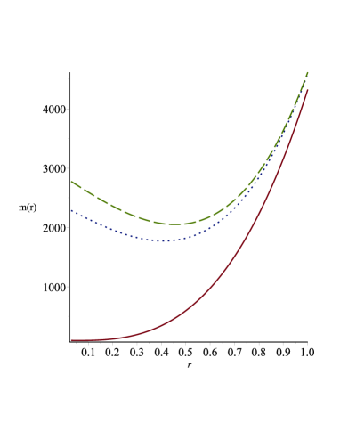
Figure 1: $m(r)$ versus $r$ for $n=9$, $\hat{\alpha}_{0}=0.5$, $\hat{\alpha}_{2}=2$, $\hat{\alpha}_{3}=5$, $\hat{\eta}_{2}=0.5$, $\hat{\eta}_{3}=0.006$, $q=20$, and $\beta=1$ (solid line), $\beta=20$ (dotted line) and $\beta=60$ (dashed line).

$$0 = n\widehat{\alpha}_{0}r_{+}^{n-1}+(n-2)\kappa r_{+}^{n-3}+(n-4)\widehat{\alpha}_{2}(\widehat{\eta}_{2}+\kappa^{2})r_{+}^{n-5}+(n-6)\widehat{\alpha}_{3}(\widehat{\eta}_{3}+3\widehat{\eta}_{2}\kappa+\kappa^{3})r_{+}^{n-7}$$ (27)

$$+\frac{4\beta^{2}r_{+}^{n-1}}{(n-1)}(1-\sqrt{1+z_{+}}).$$

This equation could not be solved analytically, but we just notice that the black hole has two horizons for $m>m_{ext},$ and possesses a naked singularity for $m<m_{ext}.$ For the solid line, one horizon exists for any value of $m$. This means that in this case Eq. (27) has no solution.

IV Black hole Thermodynamics

The Hawking temperature of the black hole could be calculated from the relation $T=(1/4\pi)(df/dr)_{r=r_{+}}$ where $r_{+}$ is the radius of the outer horizon. Substituting in this relation we obtain the temperature to be

$$T = \frac{1}{4\pi r_{+}[r_{+}^{4}+2\kappa\widehat{\alpha}_{2}r_{+}^{2}+3\widehat{\alpha}_{3}(\widehat{\eta}_{2}+\kappa^{2})]}\{nr_{+}^{6}\widehat{\alpha}_{0}+(n-2)\kappa r_{+}^{4}+(n-4)\widehat{\alpha}_{2}(\widehat{\eta}_{2}+\kappa^{2})r_{+}^{2}$$ (28)

$$+(n-6)\widehat{\alpha}_{3}(\widehat{\eta}_{3}+3\kappa\widehat{\eta}_{2}+\kappa^{3})+\frac{4\beta^{2}}{(n-1)}r_{+}^{6}(1-\sqrt{1+z_{+}})\},$$

where $r_{+}$ is the radius of the outer horizon.

In higher curvature gravity the area law of entropy, which states that the black hole entropy equals one-quarter of the horizon area is not satisfied. To calculate the entropy on the Killing horizon, we make use of Wald prescription which is applicable for any black hole solution of which the event horizon is a killing horizon Wald . This is given by the following integral on $(n-1)$-dimensional spacelike bifurcation surface

$$S=-2\pi\oint d^{n-1}x\sqrt{h}Y,\text{ \ \ \ \ \ }Y=Y^{abcd}\widehat{\varepsilon}_{ab}\widehat{\varepsilon}_{cd},\text{\ \ \ \ \ \ }Y^{abcd}=\frac{\partial\mathcal{L}}{\partial R_{abcd}}$$ (29)

in which $\mathcal{L}$ is the Lagrangian and $\widehat{\varepsilon}_{ab}$ is the binormal to the horizon. Straightforward calculations lead to the following expression for the entropy on the horizon as

$$S=\frac{\Sigma_{\kappa}(n-1)r_{+}^{n-1}}{4}\left\{\frac{1}{(n-1)}+\frac{2\kappa\widehat{\alpha}_{2}}{r_{+}^{2}(n-3)}+\frac{3\widehat{\alpha}_{3}(\kappa^{2}+\widehat{\eta}_{2})}{r_{+}^{4}(n-5)}\right\}.$$ (30)

where $\Sigma_{\kappa}$ represents the volume of nonconstant-curvature hypersurface. The first term in this expression is proportional to the area of the horizon. It is seen that topological invariants also contribute to the whole entropy of Lovelock black holes. The terms including $\widehat{\alpha}_{2}$ and $\widehat{\alpha}_{3}$ are present for the maximally symmetric horizons, while the term including $\widehat{\eta}_{2}$ represents contribution coming from the Einstein horizon.

Comparing the field equation at large values of $r$ (20) with the equation of motion of third order Lovelock equation for constant curvature horizon, one can find that the ADM mass of the black hole is

$$M = \frac{\Sigma_{\kappa}(n-1)m}{16\pi}=\frac{(n-1)\Sigma_{\kappa}}{16\pi}\{\widehat{\alpha}_{0}r_{+}^{n}+\kappa r_{+}^{n-2}+\widehat{\alpha}_{2}[\kappa^{2}+\widehat{\eta}_{2}]r_{+}^{n-4}+\widehat{\alpha}_{3}[\kappa^{3}+3\widehat{\eta}_{2}\kappa+\widehat{\eta}_{3}]r_{+}^{n-6}$$ (31)

$$+\frac{4\beta^{2}r_{+}^{n}}{n(n-1)}\left[1-\sqrt{1+z_{+}}+\frac{(n-1)z_{+}}{(n-2)}\digamma(z_{+})\right]\}.$$

Note that from the Hawking temperature (28), entropy (30) or the mass parameter (31), one can see that the case of $\beta=0$ or $q=0$ reduces to the case of uncharged Lovelock black hole with nonconstant curvature horizon as expected Farhang1 . While in the case of $\beta\rightarrow\infty$ the expressions reduce to those of charged solution in the presence of Maxwell field. The electric field $E(r)$ is defined by the relation $E(r)=-\Phi^{{}^{\prime}}(r),$ in which $\Phi(r)$ is the electric potential and is derived by integrating the electric field. For BI electromanetics the electric field is calculated to be

$$E(r)=\frac{q}{\sqrt{\frac{q^{2}}{\beta^{2}}+r^{2n-2}}},$$ (32)

from which we calculate electric potential measured at infinity with respect to the horizon is

$$\Phi=\sqrt{\frac{n-1}{2n-4}}\frac{q}{r_{+}^{n-2}}\digamma(z_{+}).$$ (33)

Also $Q$ which is called thermodynamic electric charge is related to the charge via

$$Q=\frac{q\Sigma_{\kappa}}{4\pi}\sqrt{\frac{(n-1)(n-2)}{2}}.$$ (34)

To show that the solutions we obtained above, follow the first law of thermodynamics, with the help of the following relation

$$\frac{d}{dr}(\frac{{}_{2}F_{1}\left(\left[\frac{1}{2},b\right],\left[b+1\right],-z\right)}{(n-3)r^{n-3}})=\frac{-1}{\sqrt{\frac{q^{2}}{\beta^{2}}+r^{2n-4}}},$$ (35)

and making use of thermodynamic quantities that we derived, the equation

$$dM=T\partial{S+\Phi\partial Q,}$$

is easily satisfied.

Now we are ready to study the influence of the nonlinearity of the electromagnetic field on the existence of the thermal stability of the black hole solutions. The method of performing stability of black holes of Einstein gravity may be found in Hawking ; Kastor . As we are investigating the stability in the canonical ensemble, the charge is fixed and the heat capacity is defined by the relation

$$C_{Q}=(\frac{\partial M}{\partial T})_{Q}=T(\frac{\partial S}{\partial T})_{Q}$$ (36)

An increase in temperature for fixed charge will result in an increase in the entropy leading local stability. Thus, positive heat capacity implies that the black hole is locally stable. The relation for $C_{Q}$ is complicated and we do not write it here. Instead we follow a numerical analysis. We display $C_{Q}-r_{+}$ and $T-r_{+}$ diagrams. To see the effect of the BI term on the thermodynamic of the system, first we plot temperature versus the black hole horizon $r_{+}$ in Fig. 2 for uncharged, electric charged and BI black holes. For a range of values of $q$ and $\beta$, the temperature of BI black holes has a maximum and a local minimum values at $r_{+}=r_{1}$ and $r_{+}=r_{2}$ respectively for which $\frac{dT}{dr_{+}}=0$. It is zero at $r_{+}=r_{0}$ for which extreme black hole can exist, where the value of $r_{0\text{ }}$ is getting closer to zero for BI black holes.

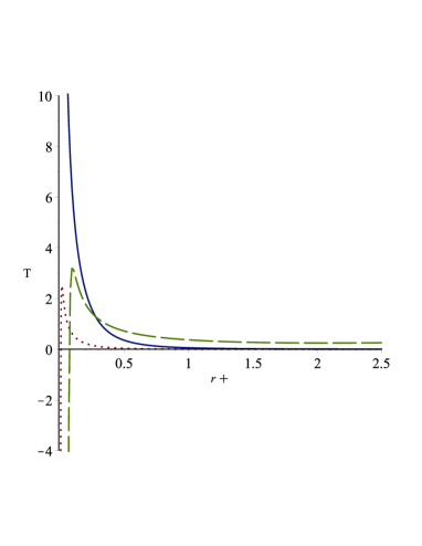
Figure 2: $T$ versus $r_{+}$ for $n=9$, $\hat{\alpha}_{0}=0.1$, $\hat{\alpha}_{2}=2$, $\hat{\alpha}_{3}=5$, $\hat{\eta}_{2}=1$ and $\hat{\eta}_{3}=5$, for uncharged solution (solid line), charged solution with $q=1$ (dashed line) and BI solution with $q=1$ and $\beta=0.5$ (dotted line).

Due to the existence of the term including $\beta,$ and $\widehat{\eta}_{3}$ that could be negative, the Hawking temperature given by the relation (28), could be negative which is unphysical. So we depict capacity as a function of $r_{+}$ in the region that temperature is positive. Considering relation (36), one can see that the heat capacity is zero at $r_{+}=r_{0}$ and blows up at $r_{+}=r_{1}$ and $r_{2}$, so the black hole has a phase transition at these points. The graphs of $T$ and $C_{Q}$ vs. $r_{+}$ are shown for positive $\kappa$ in Fig. 3. It is seen that for positive $\kappa$ small black holes ($r_{0}<$ $r_{+}<r_{1}$) and large ones ($r_{+}>r_{2}$) are stable while there exists an intermediate unstable phase with horizon area $\ r_{1}<r_{+}<r_{2}$. This case is similar to Einstein-BI and Lovelock-BI black hole with constant-curvature horizon EBI1 ; LovBI .

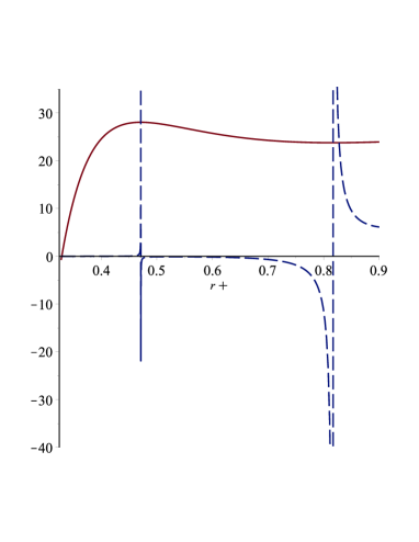
Figure 3: $T$ (solid line) and $C_{Q}$ (dashed line) versus $r_{+}$ for $n=8$, $\kappa=1$, $\hat{\alpha}_{0}=0.1$, $\hat{\alpha}_{2}=1$, $\hat{\alpha}_{3}=1/3$, $\hat{\eta}_{2}=1$, $\hat{\eta}_{3}=5$, $q=2$, and $\beta=5$.

But the case is different for $\kappa=0$. It is known that for Lovelock black holes with constant curvature horizon and $\kappa=0$, the Lovelock parameters do not appear in relation of temperature, entropy and heat capacity. Thus Lovelock correction has no contribution in the heat capacity and therefore Lovelock-BI black hole are locally stable in the whole range of $r_{+}$ EBI5 . But for our new solution, with nontrivial boundary, the existence of Lovelock coefficients in addition to the parameters that appear due to the nonconstancy of the horizon makes drastic changes to the relations. The entropy is no longer proportional to the area. For $\kappa=0$ black holes with nonconstant-curvature horizon, an unstable phase exists similar to what we explained for solutions with positive $\kappa$. To see the effect of the nonlinearity of the BI field on the stability of the black hole, first we display $C_{Q}$ versus $r_{+}$ for charged Lovelock Black hole with nonconstant-curvature horizon in the presence of the Maxwell field in Fig. 4. We see that for a chosen value of $q$ the black hole is stable in the whole range of $r_{+}.$ In Fig. 5 the heat capacity is depicted for the BI solution with the same fixed value of $q$ but for different values of $\beta$. The interesting result is that the unstable phase appears when $\beta$ is decreased. This means that nonlinearity of the field creates instability of the black hole.

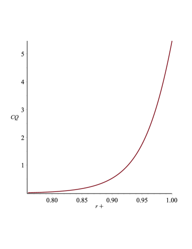
Figure 4: $C_{Q}$ versus $r_{+}$ for $n=9$, $\hat{\alpha}_{0}=0.1$, $\hat{\alpha}_{2}=1$, $\hat{\alpha}_{3}=1/3$, $\hat{\eta}_{2}=1$, $\hat{\eta}_{3}=5$, and $q=0.1$.

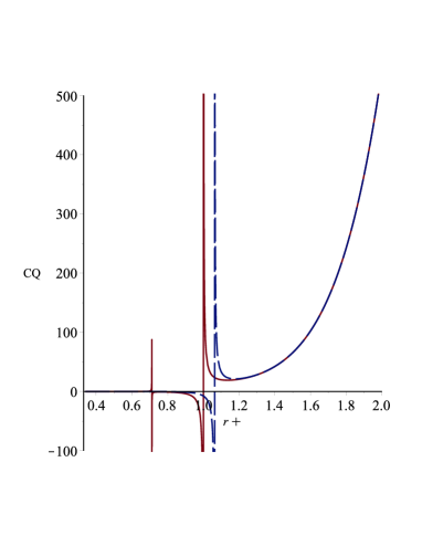
Figure 5: $C_{Q}$ versus $r_{+}$ for $n=9$, $\hat{\alpha}_{0}=0.1$, $\hat{\alpha}_{2}=1$, $\hat{\alpha}_{3}=1/3$, $\hat{\eta}_{2}=1$, $\hat{\eta}_{3}=5$, $q=0.1$, and $\beta=0.3$ (solid line), $\beta=0.1$ (dashed line) .

V Concluding Remarks

New solutions of Lovelock theory in the presence of BI field have been investigated. The horizon space consumed is nonmaximally symmetric Einstein space which has nonzero Weyl curvature. The supplementary conditions on the Weyl tensor, have a nontrivial contribution in the solution in terms of chargelike parameters. The behavior of the solutions has been presented at infinity which shows that asymptotic behavior of the solution is the same as that of uncharged solution and charged solution in the presence of Maxwell field. Thus, the matter field has no contribution in the metric function at infinity. Near the origin, the behavior of the solution is more interesting and more variety exists for the nature of the singularity of the black holes. For the special value of $m$ in eight dimensions ($n=7$) the metric function has a finite value at the origin which can be positive, negative or zero. For dimensions higher than seven ($n>6$) depending on the values of the parameters of the solution, the singularity could be spacelike resembling the solution without a matter field, or timelike which is the behaviour of singularity of the electric charged solution in the presence of the Maxwell field. We also showed that these kinds of black holes could have one or two horizons or possess naked singularity depending on the parameters of the solution. Next, we calculated thermodynamical quantities in order to investigate the stability of the black holes. Plotting temperature versus horizon radius for solutions in vacuum and in the presence of the Maxwell and BI field separately, we found that as $\beta$ increases, one may have smaller extreme black holes. By calculating the heat capacity and applying numerical analysis for positive $\kappa$, we found that small and large black hole are locally stable, while there exists an intermediate unstable phase. This is similar to the BI black holes with constant curvature horizon. Lovelock parameters do not appear in the relation of temperature, entropy and heat capacity of Lovelock black holes with flat horizon, and therefore Lovelock correction has no contribution in these variables. Thus, these kind of Lovelock-BI black hole are locally stable in the whole range of $r_{+}$ for any value of $\beta$. But, for our solutions with nonconstant curvature with $\kappa=0$, the appearance of the parameters in the thermodynamic quantities makes drastic changes in the properties of black holes in such a way that one may have unstable phase. To check the effect of the nonlinearity of the BI field, we compared the plot of heat capacity verses horizon for charged solution in the presence of Maxwell field for a fixed $q$, and then in the presence of a BI field for that fixed value of $q$ but for different values of $\beta$. The result indicates that while the black hole is stable in the whole range of $r_{+}$ in the presence of Maxwell field, or either BI field with large $\beta$, instability appears for smaller values of $\beta$, and therefore nonlinearity brings in instability.

References

- (1) B. A. Campbell, M. J. Duncan, N. Kaloper, and K. A. Olive, Nucl. Phys. B351, 778 (1991); I. Antoniadis, J. Rizos, and K. Tamvakis, Nucl. Phys. B415, 497 (1994).
- (2) L. Randall, R. Sundrum, Phys. Rev. Lett. 83, 3370 (1999); 83, 4960 (1999); G. Dvali, G. Gabadadze, and M. Porrati, Phys. Lett. B 485, 208 (2000); G. Dvali and G. Gabadadze, Phys. Rev. D 63, 065007 (2001).
- (3) D. Lovelock, J. Math. Phys. 12, 498 (1971).
- (4) B. Zwiebach, Phys. Lett. B 156, 315 (1985); D. J. Gross and J. H. Sloan, Nucl. Phys. B291, 41 (1987).
- (5) C. Bohm, Invent. Math. 134, 145 (1998).
- (6) H. Lu, D. N. Page, and C. N. Pope, Phys. Lett. B 593, 218 (2004); J. P. Gauntlett, D. Martelli, J. F. Sparks, and D. Waldram, Adv. Theor. Math. Phys. 8, 987 (2004).
- (7) G.W. Gibbons, S.A. Hartnoll, and C.N. Pope, Phys. Rev. D 67, 084024 (2003).
- (8) F. Canfora and A. Giacomini, Phys. Rev. D 82, 024022 (2010).
- (9) G. Dotti and R.J. Gleiser, Phys. Lett. B 627, 174 (2005).
- (10) G. Dotti, J. Oliva, and R. Troncoso, Phys. Rev. D 75, 024002 (2007); G. Dotti, J. Oliva, and R. Troncoso, Int. J. Mod. Phys. A 24, 1690 (2009); G. Dotti, J. Oliva, and R. Troncoso, Phys. Rev. D 82, 024002 (2010).
- (11) H. Maeda, Phys. Rev. D 81, 124007 (2010); H. Maeda, M. Hassaine, and C. Martinez, J. High Energy Phys. 08 (2010) 123.
- (12) C. Bogdanos, C. Charmousis, B. Gouteraux, and R. Zegers, J. High Energy Phys. 10 (2009) 037.
- (13) J. M. Pons and N. Dadhich, Eur. Phys. J. C 75, 280 (2015).
- (14) N. Farhangkhah and M. H. Dehghani, Phys. Rev. D 90, 044014 (2014).
- (15) S. Ray, Classical Quantum Gravity 32, 195022 (2015).
- (16) S. Ohashi and M. Nozawa, Phys. Rev. D 92, 064020 (2015).
- (17) N. Farhangkhah, Int. J. Mod. Phys. D 25, 1650030 (2016).
- (18) M. Born and L. Infeld , Nature (London) 132, 1004 (1933).
- (19) B. Hoffmann, Phys. Rev. D 47, 877 (1935).
- (20) A. Garcia, H. Salazar, and J.F. Plebanski, Nuovo. Cimento. Soc. Ital. Fis. A 84, 65 (1984); G. W. Gibbons and D. A. Rasheed, Nucl. Phys. B454, 185 (1995).
- (21) H.P. de Oliveira, Classical Quantum Gravity 11, 1469 (1994); E. Ayon-Beato and A. Garcia, Phys. Rev. Lett. 80, 5056 (1998).
- (22) Sh. Fernando, Phys.Rev. D 74, 104032 (2006).
- (23) T. Tamaki and T. Torii, Phys. Rev. D 62, 061501 (2000); G. Clement and D. Gal’tsov, Phys. Rev. D 62, 124013 (2000).
- (24) R. G. Cai, D. W. Pang, and A. Wang, Phys. Rev. D 70, 124034 (2004).
- (25) M. Aiello, R. Ferraro, and G. Giribet, Phys. Rev. D 70, 104014 (2004).
- (26) T. K. Dey, Phys. Lett. B 595, 484 (2004).
- (27) M. H. Dehghani and S. H. Hendi, Int. J. Mod. Phys. D 16, 1829 (2007); D. Zou, Z. Yang, R. Yue, and P. Li, Mod. Phys. Lett. A 26, 515 (2011).
- (28) M. Aiello, R. Ferraro, and G. Giribet, Phys. Rev. D 70, 104014 (2004); M. H. Dehghani, S. H. Hendi, A. Sheykhi, and H. Rastegar Sedehi, J. Cosmol. Astropart Phys. 02 (2007) 020; M. H. Dehghani, N. Alinejadi, and S. H. Hendi, Phys. Rev. D 77, 104025 (2008).
- (29) R. Banerjee and D. Roychowdhury, Phys. Rev. D 85, 044040 (2012).
- (30) J. X. Mo and W. B. Liu, Eur. Phys. J. C 74, 2836 (2014).
- (31) Y. S. Myung, Y. W. Kim, and Y. J. Park, Phys. Rev. D 78, 084002 (2008).
- (32) O. Miskovic and R. Olea, Phys. Rev. D 77, 124048 (2008); O. Miskovic and R. Olea, Phys. Rev. D 83, 064017 (2011); D. C. Zou, Z. Y. Yang, R. H. Yue, and P. Li, Mod. Phys. Lett. A 26, 515 (2011).
- (33) P. Li, R. H. Yue, and D. C. Zou, Commun. Theor. Phys. 56, 845 (2011).
- (34) R. C. Myers and B. Robinson, J. High Energy Phys. 08 (2010) 067.
- (35) S.W. Hawking and D. N. Page, Commun. Math. Phys. 87, 577 (1983).
- (36) R. M. Wald, Phys. Rev. D 48, R3427 (1993); V. Iyer and R. M. Wald, Phys. Rev. D 50, 846 (1994); T. Jacobson, G. Kang, and R. C. Myers, Phys. Rev. D 49, 6587 (1994).
- (37) D. Kastor, S. Ray, and J. Traschen, Classical Quantum Gravity 26, 195011 (2009).