Quantum Lattice Contraction Induced by Transient Raman Process

Abstract

The lattice contraction that occurs in time resolved x-ray diffraction and electron diffraction experiments is generally considered to be caused by photogenerated carriers. However, quantum calculations with finite-time boundary conditions indicate that a transient Raman process directly connects optical transitions and lattice displacements. Lattice contraction and coherent phonons are well explained by the Raman process.

Raman scattering is a basic quantum process that directly connects optical transitions and lattice vibrations. Since its discovery Raman and Krishnan (1928), it has been observed in various material systems and now forms the basis of a standard method to evaluate the physical properties of materials. Theoretically, Raman scattering is well explained by Fermi’s golden rule (FGR) Dirac (1927).

Advances in ultrafast laser technology enable the generation and detection of lattice vibrations (so-called ”coherent phonons”) in the time domain. Following the observation of the oscillation in acoustic waves Salcedo et al. (1978), intramolecular oscillations were also observed Silvestri et al. (1985). The latter are explained by impulsive stimulated Raman scattering (ISRS) in analogy with quantum beats Harde et al. (1981), which involve the interference of two optical transitions, where each transition is explained by the FGR. However, for ISRS, coherent phonons are represented as a coherent state that is introduced as the quantum counterpart of a classical oscillatory wave state Glauber (1963a, b). This coherent state is a highly superposed state of energy eigenstates and cannot be excited in the context of the FGR, as shown in Fig. 1(a).

Figure 1: Fermi’s golden rule applied to the generation of coherent phonons. (a) Spontaneous Raman scattering from phonon of energy $\hbar\Omega$ cannot excite the coherent phonon state centered at the $n$th phonon state. (b) Other theoretical approaches consider Newtonian forces generated by electronic excitation.

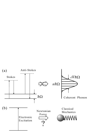
Other theoretical approaches to the generation of coherent phonons consider the Newtonian forces generated by optical transitions, as depicted in Fig. 1(b). To generate coherent phonons, previous works have proposed the impulsive force derived from the dielectric energy Merlin (1997) and the step-like force generated by a change in the equilibrium position of the lattice potential Zeiger et al. (1992). The latter process is called displacive excitation of coherent phonons (DECP). These forces seem to explain qualitatively the generation of coherent phonon oscillations described by sine and cosine functions, respectively. Conversely, the discovery of lattice contraction by time-resolved electron and x-ray diffraction experiments under high-density photoexcitation of electrons Carbone et al. (2008); Raman et al. (2008); Li et al. (2017) has given rise to even greater problems. To explain this phenomenon, we consider the strong force caused by high-density photoexcited electrons. However, to the best of our knowledge, no clear explanation is available for the photogenerated lattice displacement.

To address this issue, we introduce herein a quantum process to explain both coherent phonons and lattice contraction. We show that the deep discontinuity between the Raman scattering and the generation of coherent phonons is actually due to the temporal boundary condition in the quantum calculation.

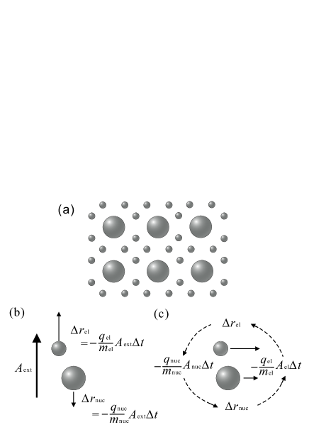
To begin, we consider the electromagnetic interaction of a crystal lattice with a laser field. Figure 2(a) shows a schematic view of the crystal composed of nuclei and electrons. The Hamiltonian of charged particle $i$ is

$${\cal H}^{(i)}=\frac{1}{2m_{i}}\left\{\vec{p}_{i}-q_{i}\left(\vec{A}_{\rm ext}(t)+\vec{A}_{i}(\vec{r}_{i})\right)\right\}^{2}+q_{i}{\phi}_{i}(\vec{r}_{i}),$$ (1)

where $m_{i}$, $q_{i}$, $\vec{r}_{i}$, and $\vec{p}_{i}$ are the mass, charge, position and conjugate momentum of particle $i$, respectively. $\vec{A}_{\rm ext}(t)$ describes the uniform long-wavelength laser field. $\phi_{i}(\vec{r}_{i})$ and $\vec{A}_{i}(\vec{r}_{i})$ are the scalar and vector electromagnetic potentials at the particle position caused by the other charged particles, respectively, and are given by

$${\phi}_{i}(\vec{r}_{i}) = \frac{1}{4\pi\varepsilon_{0}}\sum_{j\neq i}\frac{q_{j}}{|\vec{r}_{i}-\vec{r}_{j}|},$$ (2)

$$\vec{A}_{i}(\vec{r}_{i}) = \frac{1}{4\pi\varepsilon_{0}c^{2}}\sum_{j\neq i}\frac{q_{j}}{|\vec{r}_{i}-\vec{r}_{j}|}\frac{{\rm d}\vec{r}_{j}}{{\rm d}t},$$ (3)

where $\varepsilon_{0}$ and $c$ are the dielectric constant and the speed of light in vacuum, respectively.

Figure 2: Electromagnetic interaction of a crystal lattice with a laser field. (a) Schematic drawing of lattice composed of nuclei and electrons. (b) Antiphase motion of a nucleus and electron caused by direct interaction with external vector potential. (c) Additional interaction enhances the lattice displacement.

The Hamiltonian (1) may be rewritten as

$${\cal H}^{(i)}={\cal H}^{(i)}_{0}+{\cal H}^{(i)}_{\rm d}+{\cal H}^{(i)}_{\rm a},\\$$ (4)

$${\cal H}^{(i)}_{0} = \frac{1}{2m_{i}}\vec{p}_{i}^{2}+\sum_{j\neq i}\frac{1}{4\pi\varepsilon_{0}}\frac{q_{i}q_{j}}{|\vec{r}_{i}-\vec{r}_{j}|},$$ (5)

$${\cal H}^{(i)}_{{\rm d}} = -\frac{q_{i}}{m_{i}}\vec{p}_{i}\cdot\vec{A}_{{\rm ext}}(t)+\frac{q_{i}^{2}}{2m_{i}}\vec{A}^{2}_{\rm ext}(t),$$ (6)

$${\cal H}^{(i)}_{\rm a}=-\frac{q_{i}}{m_{i}}\left(\vec{p}_{i}-q_{i}\vec{A}_{\rm ext}(t)\right)\cdot\vec{A}_{i}(\vec{r}_{i})+\frac{q_{i}^{2}}{2m_{i}}\vec{A}^{2}_{i}(\vec{r}_{i}).$$ (7)

Equations (5)-(7) correspond to the free, the direct interaction, and the additional interaction Hamiltonians, respectively. The equations of motion involving $\vec{r}_{i}$ and $\vec{p}_{i}$ for each charged particles are

$$\frac{{\rm d}\vec{r}_{i}}{{\rm d}t}=\frac{\vec{p}_{i}}{m_{i}}-\frac{q_{i}}{m_{i}}\vec{A}_{\rm ext}(t)-\frac{1}{m_{i}c^{2}}\sum_{j\neq i}\frac{q_{i}q_{j}}{4\pi\varepsilon_{0}|\vec{r}_{i}-\vec{r}_{j}|}\frac{{\rm d}\vec{r}_{j}}{{\rm d}t},$$ (8)

$$\frac{{\rm d}\vec{p}_{i}}{{\rm d}t}=-\sum_{j\neq i}\left(1-\frac{1}{c^{2}}\frac{{\rm d}\vec{r}_{i}}{{\rm d}t}\cdot\frac{{\rm d}\vec{r}_{j}}{{\rm d}t}\right)\frac{\partial}{\partial\vec{r}_{i}}\frac{q_{i}q_{j}}{4\pi\varepsilon_{0}|\vec{r}_{i}-\vec{r}_{j}|}.$$ (9)

The second term on the right-hand side of Eq. (8) comes from the direct interaction Hamiltonian (6) and causes the antiphase motion of electrons and nuclei at the optical frequency, as shown in Fig. 2(b). Conversely, the third term on the right-hand side of Eq. (8) comes from Eq. (7) and is responsible for the positive feedback between the electron and the nucleus, as shown in Fig. 2(c). This term enhances the lattice displacement. The third term gives the 1/r long-range interaction network between the many charged particles, including the core electrons and the nuclei. The problem is how to quantize this many-body interaction.

In quantum mechanics, ”divergence” occurs because of the uncertainty relation. The FGR approximation Dirac (1927) is the simplest and strongest way to exclude various processes not involved in actual observations by isolating only resonant transitions between eigenstates over infinite time. However, the rule threatens to exclude processes that can actually be observed. Given the boundary conditions of finite time and space, ”divergence” causes different types of processes Stueckelberg (1950); Ishikawa and Tobita (2013); Ishikawa et al. (2015). The quantization of the electromagnetic Hamiltonian with the boundary condition of finite space leads to the Aharonov-Bohm effect Aharonov and Bohm (1959). The optical transition is also described by the vector potential, as in Eq. (6). By using the commutator relation between the coordinates and the free Hamiltonian, the amplitude of the optical transition between two energy eigenstates $|E_{\rm i}>$ and $|E_{\rm f}>$ may be rewritten as

$$\Braket{E_{\rm f}}{\frac{q}{m}\vec{p}\cdot\vec{A}_{\rm ext}}{E_{\rm i}}=\frac{\omega_{\text{fi}}}{\omega}\Braket{E_{\rm f}}{q\vec{r}\cdot\vec{E}_{\rm ext}}{E_{\rm i}},$$ (10)

where $\omega_{\rm fi}$ and $\omega$ are the transition and optical frequencies, respectively, and $\vec{E}_{\rm ext}=-\partial\vec{A}_{\rm ext}/\partial t$ is the corresponding electric field. In the FGR approximation, the momentum interaction is replaced with the electric-dipole interaction because the amplitudes are identical in resonance conditions. However, this assumption does not hold for many nonresonant transitions, which occur when time is finite Maeda et al. (2017). The vector potential causes the quantum motion of the nuclei through the momentum operators without changing the total momentum, as shown in Fig. 2(c).

Next we derive the effective Hamiltonian for the generation of coherent phonons. The lattice Hamiltonian derived from Eq. (5) determines the energy eigenstates of the lattice system, including the ground state, the electronic excited states, and the number of phonon states. The free Hamiltonian for the phonon mode is

$${\hat{\cal H}}_{0}=\frac{\hat{P}^{2}}{2M}+\frac{M\Omega^{2}}{2}\hat{R}^{2},$$ (11)

where $\hat{R}$, $\hat{P}$, $M$, and $\Omega$ are the coordinate operator, conjugate-momentum operator, mass, and phonon energy, respectively. $\hat{R}$ is the linear combination of the displacements of nuclei from their equilibrium positions. The interaction Hamiltonian derived from Eqs. (6) and (7) gives the dielectric energy of the lattice system. After averaging over an optical cycle, the corresponding complex polarizability $\hat{\chi}$ expressed in terms of phonon operators is

$$\hat{\chi}(\hat{R},\hat{P})={\chi}_{0}+\frac{\partial\tilde{\chi}}{\partial R}\hat{R}+\frac{\partial\tilde{\chi}}{\partial P}\hat{P}.$$ (12)

$\hat{\chi}$ is also a function of the laser frequency $\omega$ and contains the effects of all optical transitions. The operator $\chi_{0}$ is responsible for the generating photoexcited charge carriers. The interaction Hamiltonian for the phonon mode is

$$\hat{V}(t)=-\left(\frac{\partial\tilde{\chi}_{\rm{Re}}}{\partial R}\hat{R}+\frac{\partial\tilde{\chi}_{\rm{Re}}}{\partial P}\hat{P}\right)\overline{E_{\rm ext}^{2}(t)}.$$ (13)

If we define the phonon-annihilation operator

$$\hat{a}=\sqrt{\frac{M\Omega}{2\hbar}}\hat{R}+{\rm i}\sqrt{\frac{1}{2M\hbar\Omega}}\hat{P},$$ (14)

then the second-quantized effective Hamiltonian is

$$\hat{\cal H}_{\rm eff}(t)=\frac{\hbar\Omega}{2}\left(\hat{a}\hat{a}^{{\dagger}}+\hat{a}^{{\dagger}}\hat{a}\right)-\frac{1}{2}\left(\Xi\hat{a}+\Xi^{*}\hat{a}^{{\dagger}}\right)\overline{E_{\rm ext}^{2}(t)},$$ (15)

where the complex coefficient is

$$\Xi=\sqrt{\frac{2\hbar}{M\Omega}}\frac{\partial\tilde{\chi}_{\rm Re}}{\partial R}-{\rm i}\sqrt{2M\hbar\Omega}\frac{\partial\tilde{\chi}_{\rm Re}}{\partial P}=\frac{d\tilde{\chi}}{da}.$$ (16)

Considering $\tilde{\chi}$ to be an analytic function of $a$, Eq. (16) can be thought of as a complex derivative, so the Cauchy-Riemann equations give

$$\frac{\partial\tilde{\chi}_{\rm Re}}{\partial R}=M\Omega\frac{\partial\tilde{\chi}_{\rm Im}}{\partial P},\;\;\;\frac{\partial\tilde{\chi}_{\rm Re}}{\partial P}=-\frac{1}{M\Omega}\frac{\partial\tilde{\chi}_{\rm Im}}{\partial R}.$$ (17)

In the interaction picture, the time evolution of the phonon wave function by the Schrödinger equation gives

$$\Psi(t)={\cal{T}}\exp\left(\frac{1}{\rm{i}\hbar}\int_{t_{0}}^{t}\hat{V}_{\rm I}(t^{\prime})\overline{E^{2}(t^{\prime})}dt^{\prime}\right)\Psi(t_{0}),$$ (18)

where $\cal T$ is the time-ordering product and

$$\hat{V}_{\rm I}(t)=e^{-\frac{\hat{\cal{H}}_{0}(t-t_{0})}{\rm{i}\hbar}}\hat{V}(t)e^{\frac{\hat{\cal{H}}_{0}(t-t_{0})}{\rm{i}\hbar}}.$$ (19)

In the steady state, the perturbation integral averages to zero. If the interaction time $t-t_{0}$ is less than $1/\Omega$, the time evolution may be approximated as

$$\Psi(t)\approx\exp\left(-\frac{\Xi{\hat{a}}+\Xi^{*}\hat{a}^{{\dagger}}}{2\rm{i}\hbar}\int_{t_{0}}^{t}\overline{E_{\rm ext}^{2}(t^{\prime})}dt^{\prime}\right)\Psi(t_{0}).$$ (20)

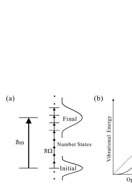
The unitary operator in Eq. (20) corresponds to the displacement operator Glauber (1963b). The coherent state is generated by applying the operator to the vacuum state, which causes the transitions from the many-number phonon states of the initial state to those of the final state, as shown in Fig. 3(a). The amplitude of each transition is very small but their sum could be very large.

Figure 3: (a) Optical transition and associated action of displacement operator on phonon-number states. (b) Vibrational energy of phonon as a function of optical fluence.

To evaluate the vibrational energy of the phonon mode, we consider the Heisenberg operator and its expectation value on the ground state. Because the time derivative is obtained from commutation with the total Hamiltonian, the rate of the vibrational energy is

$$\frac{{\rm d\Braket{0}{\hat{\cal H}_{0}}{0}}}{{\rm d}t}=\Omega\left(\frac{\partial\tilde{\chi}_{\rm Im}}{\partial P}P(t)+\frac{\partial\tilde{\chi}_{\rm Im}}{\partial R}R(t)\right)\overline{E_{\rm ext}^{2}(t)}.$$ (21)

Equations (17) are used to simplify Eq. (21). The equation shows that the increase in vibrational energy is supplied by the photon absorption induced by the lattice displacement. The absorption is essential to generating coherent phonons and was already reported in early experiments in coherent phonons Salcedo et al. (1978). The amplitude of the coherent phonon is proportional to the optical fluence and the vibrational energy of the phonon is proportional to the square of the amplitude, so the vibrational energy is proportional to the square of the fluence, as shown in Fig. 3(b). This dependence of the vibrational energy on the optical fluence is fully explained by the induced absorption. Comparing Eq. (21) with the corresponding classical optical absorption gives the relation

$$\Omega\left(\frac{\partial\tilde{\chi}_{\rm Im}}{\partial P}P+\frac{\partial\tilde{\chi}_{\rm Im}}{\partial R}R\right)=\omega\left(\frac{\partial\chi_{\rm Im}}{\partial P}P+\frac{\partial\chi_{\rm Im}}{\partial R}R\right).$$ (22)

The feedback process shown in Fig. 3(a) between optical absorption and lattice displacement is neglected in the classical theory and is indicated by the factor $\omega/\Omega$. By using the Heisenberg operator, the differential equation of the expectation value of the annihilation operator is

$$\left(\frac{\rm d}{{\rm d}t}+i\Omega\right)a=-\frac{\Xi^{*}}{2{\rm i}\hbar}\overline{E_{\rm ext}^{2}(t)}.$$ (23)

Integrating this equation from the equilibrium state gives

$$a(t)=-\frac{\Xi^{*}}{2{\rm i}\hbar}\int_{0}^{t}\overline{E_{\rm ext}^{2}(t^{\prime})}e^{{\rm i}\Omega(t-t^{\prime})}dt^{\prime}.$$ (24)

Applying Eqs. (14), (16), (17), and (22) to Eq. (24) and using the impulsive condition $t<1/\Omega$, the momentum $P$ and displacement $R$ are approximated as

$$\begin{split}P(t)&\approx\frac{\partial\chi_{\rm Re}}{\partial R}\frac{\omega}{\Omega}\int_{0}^{t}\overline{E_{\rm ext}^{2}(t^{\prime})}dt^{\prime},\\ R(t)&\approx\frac{\partial\chi_{\rm Im}}{\partial R}\frac{\omega}{M\Omega^{2}}\int_{0}^{t}\overline{E_{\rm ext}^{2}(t^{\prime})}dt^{\prime},\end{split}$$ (25)

where $\partial\chi_{\rm Re}/\partial R$ and $\partial\chi_{\rm Im}/\partial R$ are the real and imaginary parts of the classical Raman tensor. These parts correspond to the processes formerly assigned to ISRS Silvestri et al. (1985) and DECP Zeiger et al. (1992), respectively.

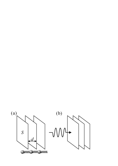
Finally, we apply the effective Hamiltonian to the ideal lattice system composed of atomic layers with a cross-sectional area $S$ and lattice constant $d$, as depicted in Fig. 4(a).

Figure 4: (a) The ideal lattice consists of atomic layers with cross sectional area $S$ and lattice constant $d$. (b) Photoexcitation causes the quantum lattice to contract without the photogeneration of carriers.

If we assume that $R$ and $P$ are the displacement of the interlayer distance and its conjugate momentum, the Hamiltonian of the monoatomic layer is

$${\cal H}_{\rm L}=\frac{P^{2}}{2\rho Sd}+\frac{YSd}{2}\left(\frac{R}{d}\right)^{2}-\frac{\omega Sd}{\Omega}\left(\frac{\varepsilon_{\rm Re}}{\partial R}R+\frac{\varepsilon_{\rm Re}}{\partial P}P\right)\frac{I(t)}{cn_{b}},$$ (26)

where $\rho$, $Y$, and $\varepsilon$ are the density, elastic constant, and relative dielectric constant, respectively. The total optical polarizability $\chi$, optical intensity $I(t)$, and the corresponding phonon frequency are, respectively,

$$\chi=Sd\varepsilon\varepsilon_{0},\;\;I(t)=\varepsilon_{0}n_{\rm b}^{2}\overline{E_{\rm ext}^{2}(t)}c/n_{\rm b},\;\,\Omega=\sqrt{Y/\rho}/d,$$ (27)

where $n_{\rm b}$ is the index of refraction of the crystal. We consider the change in interlayer distance in the impulsive limit $(t<1/\Omega)$. In addition, because the acoustic velocity $v=\Omega d$, acoustic propagation is limited by the lattice constant $d$, so that each atomic layer is mechanically decoupled. Replacing the parameter of Eq. (25) with the parameter of the lattice Hamiltonian Eq. (26), the lattice displacement is

$$R\approx\frac{\partial\varepsilon_{\rm Im}}{\partial R}\frac{\omega d^{2}}{Ycn_{b}}\int_{0}^{t}I(t^{\prime})dt^{\prime}.$$ (28)

For simplicity, the index $n_{b}$ of refraction is held constant. If the imaginary Raman tensor is negative, the equation gives a quantum lattice contraction, as shown in Fig. 4(b). By using a lattice strain $u=-R/d$, a vacuum laser wavelength $\lambda=2\pi c/\omega$, and an optical fluence

$$F=\int_{0}^{t}I(t^{\prime})dt^{\prime},$$ (29)

the useful expression for the associated stress $\sigma$ is

$$\sigma=Yu\approx\frac{1}{n_{\rm b}}\frac{\partial\varepsilon_{\rm Im}}{\partial u}\frac{2\pi F}{\lambda}.$$ (30)

A fluence of $\rm{10mJ/cm^{2}}$ at 800 nm corresponds to $2\pi F/\lambda$ of 0.785 GPa. The remaining part of Eq. (30) is a dimensionless quantity of order unity.

In conclusion, we derive herein the effective Hamiltonian describing an optical-lattice interaction by using the complex Raman tensor and applying a finite-time boundary condition. The optical transition and lattice displacement are tightly linked by the transient interaction caused by the vector potential so that the lattice-induced absorption takes place. The non-Newtonian momentum interaction explains the lattice contraction and the coherent-phonon generation formerly attributed to DECP. For further progress in this field, we encourage the lattice contraction and the induced photoabsorption to be verified qualitatively and quantitatively by experiment.

The author thanks Professor Kenzo Ishikawa for encouragement and stimulating discussions.

References

- Raman and Krishnan (1928) C. V. Raman and K. S. Krishnan, Nature 121, 501 (1928).
- Dirac (1927) P. A. M. Dirac, Proc. Roy. Soc. A114, 243 (1927).
- Salcedo et al. (1978) J. R. Salcedo, A. E. Siegman, D. D. Dlott, and M. D. Fayer, Phys. Rev. Lett. 41, 131 (1978).
- Silvestri et al. (1985) S. D. Silvestri, J. G. Fujimoto, E. P. Ippen, E. B. GambleJr., L. R. Williams, and K. A. Nelson, Chem. Phys. Letters 116, 146 (1985).
- Harde et al. (1981) H. Harde, H. Burggraf, J. Mlynek, and W. Lange, Opt. Lett. 6, 290 (1981).
- Glauber (1963a) R. J. Glauber, Phys. Rev. 130, 2529 (1963a).
- Glauber (1963b) R. J. Glauber, Phys. Rev. 131, 2766 (1963b).
- Merlin (1997) R. Merlin, Solid State Commun. 102, 207 (1997).
- Zeiger et al. (1992) H. J. Zeiger, J. Vidal, T. K. Cheng, E. P. Ippen, G. Dresselhaus, and M. S. Dresselhaus, Phys. Rev. B 45, 768 (1992).
- Carbone et al. (2008) F. Carbone, P. Baum, P. Rudolf, and A. H. Zewail, Phys. Rev. Lett. 100, 035501 (2008).
- Raman et al. (2008) R. K. Raman, Y. Murooka, C.-Y. Ruan, T. Yang, S. Berber, and D. Tománek, Phys. Rev. Lett. 101, 077401 (2008).
- Li et al. (2017) R. Li, O. A. Ashour, J. Chen, H. E. Elsayed-Ali, and P. M. Rentzepis, J. Appl. Phys. 121, 055102 (2017).
- Stueckelberg (1950) E. C. G. Stueckelberg, Phys. Rev. 81, 130 (1950).
- Ishikawa and Tobita (2013) K. Ishikawa and Y. Tobita, Prog. Theor. Exp. Phys. 2013, 073B02 (2013).
- Ishikawa et al. (2015) K. Ishikawa, T. Tajima, and Y. Tobita, Prog. Theor. Exp. Phys. 2015, 013B02 (2015).
- Aharonov and Bohm (1959) Y. Aharonov and D. Bohm, Phys. Rev. 115, 485 (1959).
- Maeda et al. (2017) N. Maeda, T. Yabuki, Y. Tobita, and K. Ishikawa, Prog. Theor. Exp. Phys. 2017, 053J01 (2017).