Quantum phase transition without gap opening
Abstract
Quantum phase transitions (QPTs), including symmetry breaking and topological types, always associated with gap closing and opening. We analyze the topological features of the quantum phase boundary of the XY model in a transverse magnetic field. Based on the results from graphs in the auxiliary space, we find that gapless ground states at boundary have different topological characters. On the other hand, In the framework of Majorana representation, the Majorana lattice is shown to be two coupled SSH chains. The analysis of the quantum fidelity for the Majorana eigen vector indicates the signature of QPT for the gapless state. Furthermore numerical computation shows that the transition between two types of gapless phases associates with divergence of second-order derivative of groundstate energy density, which obeys scaling behavior. It indicates that a continues QPT can occur among gapless phases. The underlying mechanism of the gapless QPT is also discussed. The gap closing and opening are not necessary for a QPT.
I Introduction
Understanding phase transitions is one of challenging tasks in condensed matter physics. No matter which types of a quantum phase transition (QPT), the groundstate wave function undergoes qualitative changes S. Sachdev . There are various signature phenomena manifest the critial points, such as symmetry breaking, switch of topological invariant, divergence of entanglement, etc.. Among them, energy gap closing and opening seem never absent. It is important for a deeper understanding of QPTs to find out the role of the energy gap takes during the transition. Usually, a continuous QPT is characterized by a divergence in the second derivative of the groundstate energy density, assuming that the first derivative is discontinuous Vojta ; Suzuki ; Dutta2 . A natural question is whether the gap closing and opening are necessary for a QPT. The aim of this paper is to clarify the relation between gap and a second-order QPT through a concrete system. We take a 1D quantum model with a transverse field, which can be mapped onto the system of spinless fermions with -wave superconductivity. It plays an important role both in traditional and symmetry-protected topological QPTs, received intense study in many aspects G. Chen ; X. X. Yi ; Zanardi ; Chenshu1 ; Chenshu2 ; Tao Liu ; Ka-Di Zhu ; WXG ; Fulibin1 ; Fulibin2 ; Fulibin3 ; Ling-Bao Kong ; Carollo ; Zhu1 ; Zhu2 .
The quantum phase boundary of the model is well known based on the exact solution. However, it mainly arises from the condition of zero energy gap. There are many other signatures to identify the critical point, such as the quantities of the ground state from the point of view of quantum information theory Osterloh , the ground-state fidelity susceptibility Zanardi ; Chandra ; De Grandi ; Chen ; Tribedi ; Rams ; Cardy ; Abanin . Then the ground states at different locations of the boundary may belong to different quantum phases, although they are not protected by a finite energy gap. In this paper, we are interested in the possible QPT along the boundary, at which the ground state is always gapless state. Our approach consists of three steps: Bogoliubov energy band, Majorana fidelity, and finite-size scaling. Firstly, we use Bogoliubov energy band to construct a group of graphs that can capture the charaters of quantum phases in every regions, including all the boundaries, which indicate the distinctions of boundaries. Secondly, we employ the fidelity of Majorana eigen vector to detect the QPT between two gapless phases. Thirdly, we investigate the scaling behavior of the critical region to show a gapless QPT has the same performance as a standard continuous QPT. The result indicates that a continues QPT can occur among gapless phases. The gap closing and opening are not necessary for a QPT.
This paper is organized as follows. In Section II, we present the model Hamiltonian and the quantum phase diagram. In Section III, we investigate the phase diagram based on the geometric properties. Section IV gives the connection between the model to a simpler lattice model by Majorana transformation. In Section V, we present the scaling behavior about the groundstate energy density to demonstrate the characteristic of continuous QPT among the gapless phases. Finally, we give a summary and discussion in Section VI.
II Model and phase diagram
We consider a 1D spin- model in a transverse magnetic field on -site lattice. The Hamiltonian has the form
| (1) |
where ( ) are the Pauli operators on site , and satisfy the periodic boundary condition .
Now we consider the solution of the Hamiltonian of Eq. (1). We start by taking the Jordan-Wigner transformation P. Jordan
| (2) |
to replace the Pauli operators by the fermionic operators . The parity of the number of fermions
| (3) |
is a conservative quantity, i.e., , where . Then the Hamiltonian (1) can be rewritten as
| (4) |
where
| (5) |
is the projector on the subspaces with even () and odd () . The Hamiltonian in each invariant subspaces has the form
| (6) | |||||
Taking the Fourier transformation
| (7) |
for the Hamiltonians , we have
| (8) | |||||
where the momenta , , . Employing the Bogoliubov transformation
where
| (9) |
one can recast Hamiltonian to the diagonal form
| (10) |
with spectrum being
| (11) |
The lowest energy in subspace is for , while for . The groundstate energy for finite is the foundation for the analysis of scaling behavior in the Sec. V. In the thermodynamical limit, the difference between two subspaces can be neglected and the groundstate energy density can be expressed as
| (12) |
by taking . The quantum phase boundary can be obtained from as
| (13) |
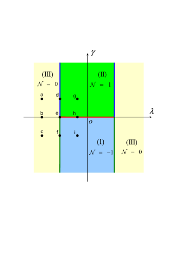
The phase diagram is presented in Fig. 1. There are four regions separated by five lines as boundaries of quantum phases. In the next section, quantum phases and boundaries will be examined from the geometrical point of view.
III Topological invariants
In this section, we will investigate the topological characterization for the phase diagram. We demonstrate this point by rewriting the Hamiltonian in the form
| (14) |
where
| (15) |
The core matrix can be expressed as
| (16) |
where the components of the auxiliary field are
| (17) |
The Pauli matrices are taken as the form
| (18) |
The winding number of a closed curve in the auxiliary -plane around the origin is defined as
| (19) |
where the unit vector . is an integer representing the total number of times that curve travels counterclockwise around the origin. Actually, the winding number is simply related the loop described by equation
| (20) |
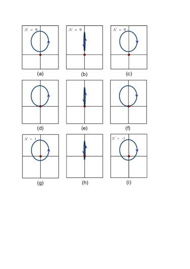
which presents a normal ellipse in the -plane. The shape and rotating direction of the ellipse dictated by the parameter equation (17) have the following symmetries. First of all, taking , we have , representing the same ellipse but with opposite rotating direction. Secondly, taking , we have , representing the same ellipse but with a shift in , while the shift cannot affect the relation between the graph and the origin. We plot several graphs at typical positions in Fig. 2 to demonstrate the features of different phases from the geometric point of view. We are interested in the loops for the parameters at the boundaries in Eq. (13). (i) For and , the ellipse always passes through the origin one time. Along the boundary, only the length of the semiaxis of the ellipse changes. (ii) For and , the loop reduces to a segment, passing through the origin twice times. Along the boundary, only the length of the segment varies. According to the connection between loops and QPTs Gang , when a loop passes through the origin, the first derivative of groundstate energy density experiences a non-analytical point. In general, this process is associated with a gap closing. However, we note that when parameters vary along and pass through , there is always one point in the curve at the origin, while the ellipse becomes a segment. In the Appendix, we show that such a system also experiences a non-analytical point but without associated gap closing and opening.
IV Majorana ladder
In this section, we investigate the phase diagram from alternative way, which gives a clear physical picture by connecting the obtained results to the previous work. In contrast to last section, where a graph is extracted from the Bogoliubov energy band, we will mark the phase diagram from the behavior of wave functions. For quantum spin model, Majorana representation always make things simpler since it can map a Kitaev model (like the form in Eq. (8)) to a lattice model in a real space with the twice number of site of the spin system Kitaev . The bulk-edge correspondence has demonstrated this advantage M. Z. Hasan .
We introduce Majorana fermion operators
| (21) |
which satisfy the relations
| (22) |
The inverse transformation is
| (23) |
Then the Majorana representation of the Hamiltonian is
| (24) | |||||
To make the structure of Majorana lattice clear, we write down the Hamiltonian in the basis and see that
| (25) |
where represents a matrix. Here matrix is explicitly written as
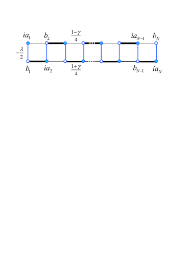
| (26) |
where basis is an orthonormal complete set, . The basis array is , which accords with . Schematic illustrations for structures of are described in Fig. 3. The structure is clearly two coupled SSH chains. The situation with corresponds to the case with half quanta flux through the double SSH rings. In the previous work Li , the gapless states in two coupled SSH chains with has been studied. It is shown that the quantum phase boundary for corresponds to topological gapless states, while boundaries are trivial topological gapless states. The joints are boundaries separated the gapless phases with different topological characterizations. We refer these points as transition point between two gapless phases.
Majorana matrix in Eq. (26) with dimension contains all the information of the original in Eq. (1) with dimension. Although the eigen vectors of have direct relation to the ground state of , it is expected that the signature of QPT between gapless phases can be manifested from them. We will investigate the change of the eigen vector of along . By the similar procedure, the eigen problem of the equation
| (27) |
with , can be solved as
| (28) |
with the eigen value
| (29) |
Here the parameter is defined as
| (30) |
We focus on the vectors with negative eigen values and taking .
We employ the quantum fidelity to detect the sudden change of the eigen vectors, which is defined as
| (31) |
i.e., the modulus of the overlap between two neighbor vectors with . Direct derivation shows that
| (32) | |||||
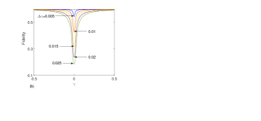
We note that the minimum of always locates at for any values of , leading to the minimum of . It indicates that the fidelity approach can be employed for Majorana eigen vector to witness the sudden change of ground state.
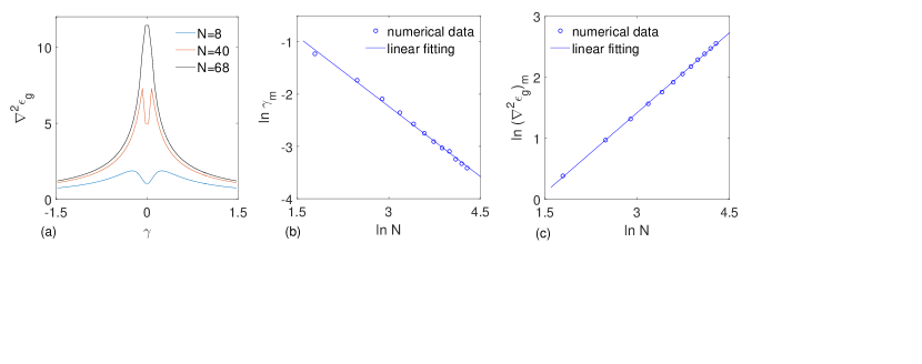
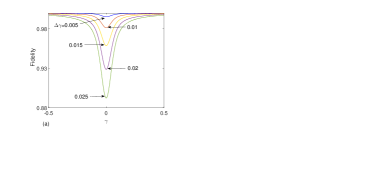
Fig. 4 shows the fidelity of for a given finite system as a function of with various parameter difference . As expected, the point is clearly marked by a sudden drop of the value of fidelity. The behavior can be ascribed to a dramatic change in the structure of the Majorana vector, indicating the QPT at zero .
V Scaling behavior
In this section, we investigate what happens for the groundstate energy when a gapless QPT occurs. The non-analytical point of energy density is more fundamental to judge the onset of a QPT. We start from the line with , on which the density of groundstate energy in thermodynamic limit has the form
| (33) |
where we neglect the difference between and . The first derivative of groundstate energy density with the respect to reads
| (34) |
where the integrand is defined as
| (35) |
We are interested in the divergent behavior of when . We note that the main contribution to the integral of comes from the region with . The contribution to from this region is approximately
| (36) |
which predicts that the first derivative of groundstate energy density along has a non-analytical point at . It is the standard characterization of second order QPT. It is crucial to stress that such phase separation does not arise from the gap closing and opening.
To characterize the behavior of groundstate energy in D parameter space, we calculate the Laplacian of
| (37) |
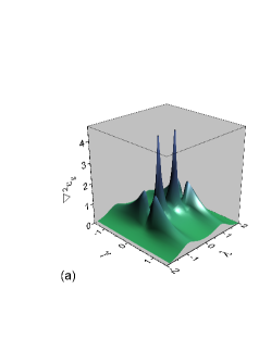
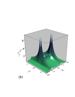
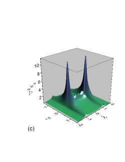
which will reduce to second derivative of the groundstate energy density of the standard transverse-field Ising model S. Sachdev with respect to the transverse field when we take . In Fig. 5 we plot the Laplacian of for the finite sized systems. We observe that as increases, the regions of criticality are clearly marked by a sudden increase of the value of . Remarkably, there are higher order sudden increases around the points . As before in a conventional QPT with gap closing and opening, for instance the QPTs at along , we ascribe this type of behavior to a dramatic change in the structure of the gapless ground state. The system undergoes a QPT along the boundary.
In order to quantify the change of the ground state when the system crosses the critical point, we look at the value of as a function of for finite size system. The results for systems of different size are presented in Fig. 6. We find the similar scaling behavior for such kinds of QPT, which reveals the fact that the signature of a second order QPT must not require the gap closing.
VI Summary and discussion
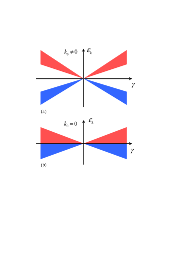
In summary, we have studied the the necessity of the energy gap closing and opening for the presence of a QPT. We focused on the joint of three types of gapless phases. The analysis based on the geometry of the ground state and Majorana representation indicate the distinction of the gapless phases. Numerical computation for finite size system shows that the transitions among the gapless phases exhibit scaling behavior, which has been regarded as the fingerprint of continuous QPT. This provides an example to demonstrate that energy gap closing and opening is not a necessary condition for the QPT. Mathematically, the existence of a gap depends on the function of dispersion relation, specifically, the upper bound of the negative band. The divergence of the second-order derivative of groundstate energy density arises from the non-analytical point of the groundstate energy, which is the summation of all negative energy levels. On the other hand, a typical negative energy level with non-analytical point is a simple level crossing at zero energy, for example, levels from matrix for . The energy gap , which is zero only at , for nonzero . However, the energy gap always vanishes for zero . We plot the spectrum for and , in Fig. 7 to illustrate this point.
VII Appendix
In this appendix, we demonstrate the existence of gapless QPT through a toy model. We consider a Hamiltonian with a specific dispersion relation for Bogoliubov band, where describes a rectangle with width and length in -plane (see Fig. 8). Here we use a rectangle to replace a ellipse in Eq. (20) in order to simplify the derivation. In the case of , the main contribution to the energy is the at the long sides. The parameter equations of the two long sides is
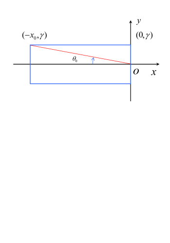
| (38) |
where is determined by tan. The energy density can be expressed as
| (39) | |||||
We note that the derivative of
| (40) |
has a jump at zero , indicating the critical point of QPT.
Acknowledgements.
We acknowledge the support of the CNSF (Grant No. 11374163).References
- (1) S. Sachdev, Quantum Phase Transition (Cambridge University Press, Cambridge, 1999).
- (2) M. Vojta, Rep. Prog. Phys. 66, 2069 (2003).
- (3) S. Suzuki, Inoue, J. I. and Chakrabarti, B. K. Quantum Ising Phases and Transitions in Transverse Ising Models Vol. 862 (Lecture Notes in Physics, Springer, 2013).
- (4) Dutta, Quantum Phase Transitions in Transverse Field Spin Models: From Statistical Physics to Quantum Information (Cambridge University Press, Cambridge, 2015)
- (5) G. Chen, J. Q. Li, and J. Q. Liang, Phys. Rev. A 74, 054101 (2006).
- (6) X. X. Yi and W. Wang, Phys. Rev. A 75, 032103 (2007).
- (7) L. C. Venuti and P. Zanardi, Phys. Rev. Lett. 99, 095701 (2007).
- (8) Yu-Quan Ma and Shu Chen, Phys. Rev. A 79, 022116 (2009).
- (9) Yu-Quan Ma, Shu Chen, Heng Fan, and Wu-Ming Liu, Phys. Rev. B 81, 245129 (2010).
- (10) Tao Liu, Yu-Yu Zhang, Qing-Hu Chen, and Ke-Lin Wang, Phys. Rev. A 80, 023810 (2009).
- (11) Xiao-Zhong Yuan, Hsi-Sheng Goan, and Ka-Di Zhu, Phys. Rev. A 81, 034102 (2010).
- (12) Xiao-Ming Lu and Xiaoguang Wang, Europhys. Lett. 91, 30003 (2010).
- (13) Sheng-Chang Li, Li-Bin Fu, and Jie Liu, Phys. Rev. A 84, 053610 (2011).
- (14) Li-Da Zhang and Li-Bin Fu, Europhys. Lett. 93, 30001 (2011).
- (15) Sheng-Chang Li and Li-Bin Fu, Phys. Rev. A 84, 023605 (2011).
- (16) Zi-Gang Yuan, Ping Zhang, Shu-Shen Li, Jian Jing, and Ling-Bao Kong, Phys. Rev. A 85, 044102 (2012).
- (17) A. C. M. Carollo and J. K. Pachos, Phys. Rev. Lett. 95, 157203 (2005).
- (18) S. L. Zhu, Phys. Rev. Lett. 96, 077206 (2006).
- (19) S. L. Zhu, Int. J. Mod. Phys. B 22, 561 (2008).
- (20) Osterloh, A., Amico, L., Falci, G. & Fazio, R., Nature 4146, 608–610, (2002).
- (21) Chandra, A. K., Das, A. and Chakrabarti, B. K., Vol. 802 (Lecture Notes in Physics, Springer, 2010).
- (22) C. De Grandi, V. Gritsev, and A. Polkovnikov, Phys. Rev. B 81, 012303 (2010).
- (23) S. Chen, L. Wang, Y. Hao, and Y. Wang, Phys. Rev. A 77, 032111 (2008).
- (24) A. Tribedi, and I. Bose, Phys. Rev. A 77, 032307 (2008).
- (25) Rams, M. M. and Damski, B., Phys. Rev. Lett. 106, 055701 (2011).
- (26) Cardy, J., Phys. Rev. Lett. 106, 150404 (2011).
- (27) Abanin, D. A. and Demler, E. Phys. Rev. Lett. 109, 020504 (2012).
- (28) P. Jordan and E. Wigner, Z. Physik 47, 631 (1928).
- (29) G. Zhang and Z. Song, Phys. Rev. Lett. 115, 177204 (2015).
- (30) A. Y. Kitaev, Phys. Usp. 44, 131 (2001).
- (31) M. Z. Hasan and C. L. Kane, Rev. Mod. Phys. 82, 3045 (2010).
- (32) C. Li, S. Lin, G. Zhang, and Z. Song, Phys. Rev. B 96, 125418 (2017).