Recursive Soft Drop

Abstract

We introduce a new jet substructure technique called Recursive Soft Drop, which generalizes the Soft Drop algorithm to have multiple grooming layers. Like the original Soft Drop method, this new recursive variant traverses a jet clustering tree to remove soft wide-angle contamination. By enforcing the Soft Drop condition $N$ times, Recursive Soft Drop improves the jet mass resolution for boosted hadronic objects like $W$ bosons, top quarks, and Higgs bosons. We further show that this improvement in mass resolution persists when including the effects of pileup, up to large pileup multiplicities. In the limit that $N$ goes to infinity, the resulting groomed jets formally have zero catchment area. As an alternative approach, we present a bottom-up version of Recursive Soft Drop which, in its local form, is similar to Recursive Soft Drop and which, in its global form, can be used to perform event-wide grooming.

1 Introduction

As the Large Hadron Collider (LHC) collides protons at the highest energies accessible in a laboratory setting, electroweak-scale resonances are routinely produced with transverse momenta far exceeding their rest mass. These highly boosted objects will generate collimated hadronic decays, which are often reconstructed as a single fat jet. Due to the differences in their radiation patterns, fat jets originating from boosted objects can be distinguished from ordinary quark and gluon jets by studying their substructure. Since the start of the experimental program of the LHC, jet substructure has matured into a highly active field of research Abdesselam:2010pt ; Altheimer:2012mn ; Altheimer:2013yza ; Adams:2015hiv ; Cacciari:2015jwa ; Larkoski:2017jix ; LH2017 . First introduced in the pioneering studies of Refs. Seymour:1991cb ; Seymour:1993mx ; Butterworth:2002tt ; Butterworth:2007ke , jet substructure was revived by seminal work showing its potential application in the search for a light Higgs boson decaying to bottom quarks Butterworth:2008iy .

By now, a variety of tools use jet substructure to tag boosted objects and mitigate contamination from poorly modeled contributions such as underlying event and pileup Thaler:2008ju ; Kaplan:2008ie ; Krohn:2009th ; Ellis:2009su ; Ellis:2009me ; Plehn:2009rk ; Kim:2010uj ; Thaler:2010tr ; Thaler:2011gf ; Larkoski:2013eya ; Chien:2013kca ; Larkoski:2014gra ; Moult:2016cvt ; Feige:2012vc ; Field:2012rw ; Dasgupta:2013ihk ; Dasgupta:2013via ; Larkoski:2014pca ; Dasgupta:2015yua ; Seymour:1997kj ; Li:2011hy ; Larkoski:2012eh ; Jankowiak:2012na ; Chien:2014nsa ; Chien:2014zna ; Isaacson:2015fra ; Krohn:2012fg ; Waalewijn:2012sv ; Larkoski:2014tva ; Larkoski:2014wba ; Procura:2014cba ; Bertolini:2015pka ; Bhattacherjee:2015psa ; Larkoski:2015kga ; Dasgupta:2015lxh ; Dasgupta:2016ktv ; Salam:2016yht ; Frye:2016okc ; Frye:2016aiz ; Kang:2016ehg ; Hornig:2016ahz ; Marzani:2017mva ; Marzani:2017kqd ; Chien:2017xrb ; Chien:2018dfn , which have already found numerous experimental applications Chatrchyan:2013vbb ; Aad:2013gja ; Khachatryan:2014vla ; Chatrchyan:2012sn ; CMS:2013cda ; Aad:2015cua ; Aad:2015lxa ; ATLAS-CONF-2015-035 ; Aad:2015rpa ; Aad:2015hna ; ATLAS-CONF-2016-002 ; ATLAS-CONF-2016-039 ; ATLAS-CONF-2016-034 ; CMS-PAS-TOP-16-013 ; CMS-PAS-HIG-16-004 ; CMS:2011bqa ; Fleischmann:2013woa ; Pilot:2013bla ; TheATLAScollaboration:2013qia ; Chatrchyan:2012ku ; CMS-PAS-B2G-14-001 ; CMS-PAS-B2G-14-002 ; Khachatryan:2015axa ; Khachatryan:2015bma ; Aad:2015owa ; Aaboud:2016okv ; Aaboud:2016trl ; Aaboud:2016qgg ; ATLAS-CONF-2016-055 ; ATLAS-CONF-2015-071 ; ATLAS-CONF-2015-068 ; CMS-PAS-EXO-16-037 ; CMS-PAS-EXO-16-040 ; Khachatryan:2016mdm ; CMS-PAS-HIG-16-016 ; CMS-PAS-B2G-15-003 ; CMS-PAS-EXO-16-017 . One particular technique that has emerged both as a powerful substructure probe and as an analytically tractable approach is the modified Mass Drop Tagger (mMDT) Dasgupta:2013ihk , and its later extension, Soft Drop (SD) Larkoski:2014wba . The SD procedure takes an initial jet with radius $R_{0}$, reclusters its constituents with the Cambridge/Aachen (C/A) algorithm Dokshitzer:1997in ; Wobisch:1998wt , and removes soft wide-angle emissions that do not satisfy the SD condition, defined as

$$\frac{\min(p_{t,1},p_{t,2})}{p_{t,1}+p_{t,2}}>z_{\text{cut}}\left(\frac{\Delta R_{12}}{R_{0}}\right)^{\beta}\,,$$ (1)

where the notation will be reviewed below. This method has been used in a variety of analyses at the LHC, including jet mass and transverse momentum measurements in dijet events CMS-PAS-SMP-16-010 ; Aaboud:2017qwh , vector resonance and dark matter searches Sirunyan:2017dnz ; Aaboud:2017eta ; Sirunyan:2018ivv ; Sirunyan:2018gka , and boosted $H\rightarrow b\bar{b}$ searches Sirunyan:2017dgc . It has also been used as a powerful probe of the QCD splitting function, both in proton-proton collision Larkoski:2017bvj ; Tripathee:2017ybi and in heavy ion collisions Sirunyan:2017bsd ; Caffarri:2017bmh ; Kauder:2017mhg , where the shared momentum fraction $z_{g}$ provides a handle on medium effects Chien:2016led ; Milhano:2017nzm ; Mehtar-Tani:2016aco . Because grooming with mMDT/SD removes complications due to unassociated wide-angle emissions, it has also allowed analytic calculations of the groomed jet mass to reach unprecedented accuracies Frye:2016okc ; Frye:2016aiz ; Marzani:2017mva ; Marzani:2017kqd .

In this paper, we introduce a recursive extension of the SD algorithm—aptly named Recursive Soft Drop (RSD)—where SD is reapplied along the C/A clustering history until a specified number $N$ of SD conditions have been satisfied. We focus on jet grooming with RSD, taking an angular exponent $\beta\geq 0$. The case $N=0$ involves no jet grooming, the case $N=1$ corresponds to the original SD procedure, and the cases $N\geq 2$ are well-suited to multi-prong boosted objects. Like the original SD, RSD is stable under hadronization and underlying event effects, but RSD is able to provide improved jet mass resolution for signals such as boosted 2-prong $W$ bosons, 3-prong top quarks, and 4-prong Higgs bosons. Intriguingly, in the $N\to\infty$ limit, groomed jets from RSD formally have zero catchment area Cacciari:2008gn , a feature that suggests that RSD would be well suited for pileup mitigation.

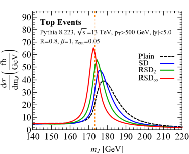
(a)

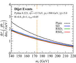
(b)

Figure 1: Behavior of RSD in (a) boosted top signals and (b) corresponding dijet backgrounds, using Pythia 8.223 and $R=0.8$ anti-$k_{t}$ jets. The benchmark SD condition in Eq. (1) uses $\beta=1$ and $z_{\text{cut}}=0.05$.

We focus our attention here on the phenomenological applications of RSD, leaving a detailed study of its analytical properties to future work. The behavior of RSD is summarized in Fig. 1 in the case of distinguishing boosted top quark signals from quark/gluon jet backgrounds. As the number of RSD layers increases, the top mass peak is better resolved, with the best performance (for this choice of SD condition) achieved in the infinite $N$ limit, hereafter labeled RSD_∞. For quark/gluon jets, RSD has a much smaller impact on the groomed mass, but there are still substantial gains in top tagging performance just from the increased signal mass resolution. In general, any application at the LHC suitable for SD is also suitable for RSD, with the possibility of loosening the SD condition while increasing the number of layers $N$ to balance performance and robustness. As a concrete example, we show how to use RSD_∞ in combination with either the SoftKiller Cacciari:2014gra or the area–median method Cacciari:2007fd ; Cacciari:2008gn to mitigate pileup in high-luminosity conditions.

The rest of this paper is organized as follows. We introduce the RSD algorithm in Sec. 2, and describe its basic features in Sec. 3, such as its robustness to non-perturbative effects and the $N\rightarrow\infty$ limit of zero-area jets. In Sec. 4, we show how RSD improves jet mass resolution for boosted resonances with hadronic decays, and we present a brief case study of boosted top tagging. In Sec. 5, we discuss the application of RSD to pileup mitigation. We present an alternative version of the RSD algorithm in Sec. 6, where a bottom-up strategy can be applied locally (at the jet level) or globally (at the event level). We conclude in Sec. 7, leaving additional studies to the appendices.

2 The Recursive Soft Drop algorithm

Since RSD is a generalization of SD, we first summarize the SD algorithm Larkoski:2014wba in Sec. 2.1, and introduce the multi-layer RSD_N algorithm in Sec. 2.2. We present a more aggressive RSD variant in Sec. 2.3. Like all jet grooming procedures, RSD_N removes wide-angle soft radiation within a jet, with the new feature that the meaning of “wide angle” is determined recursively.

2.1 Review of Soft Drop

The original SD algorithm starts from any jet, where the constituents are reclustered into a C/A angular-ordered tree Dokshitzer:1997in ; Wobisch:1998wt . The degree of jet grooming depends on two parameters: the minimum energy fraction $z_{\text{cut}}$ allowed for the softer branch, and an angular exponent $\beta$ defining how much collinear radiation is removed by the grooming procedure. It is also convenient to introduce a reference angular scale $R_{0}$ (absorbable into the definition of $z_{\text{cut}}$), which is typically set to the initial jet clustering radius $R$. We denote by $p_{t,i}$ the transverse momentum of the $i$-th subjet, and by $\Delta R_{ij}$ the rapidity-azimuth distance between the $i$-th and $j$-th subjets.

The SD algorithm proceeds as follows:

1. Undo the last C/A clustering step of the jet $j$ and label the two parent subjets as $j_{1}$ and $j_{2}$.

2. If these subjets pass the SD condition,

   $$z_{12}>z_{\text{cut}}\left(\frac{\Delta R_{12}}{R_{0}}\right)^{\beta}\,,\qquad z_{12}\equiv\frac{\min(p_{t,1},p_{t,2})}{p_{t,1}+p_{t,2}},$$ (2)

   then the procedure stops and the SD jet $j$ is returned.

3. Otherwise, the softer subjet (by $p_{t}$) is removed and the algorithm iterates on the new jet $j$ defined by the harder subjet.

4. If $j$ has no further subjets, either terminate without returning a jet (tagging mode) or define $j$ to be the SD jet (grooming mode).

As explained in Ref. Larkoski:2014wba , this algorithm is infrared and collinear (IRC) safe for $\beta>0$ in grooming mode, though it remains Sudakov safe Larkoski:2013paa ; Larkoski:2015lea for $\beta\rightarrow 0$. The limits $z_{\text{cut}}\rightarrow 0$ or $\beta\rightarrow\infty$ return an ungroomed jet. Finally, the limit $\beta\to 0$ corresponds to mMDT Dasgupta:2013ihk .

2.2 Introducing Recursive Soft Drop

As depicted in Fig. 2, RSD_N grooms a jet by applying $N$ layers of SD declustering, iterating through the full jet clustering tree. This is achieved by ordering all branches by the $\Delta R_{ij}$ separation of their constituents, and iterating through the tree structure by taking the branch with the most widely-separated constituents at each step.

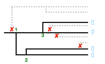
Figure 2: Schematic depiction of the RSD_N algorithm, where a C/A clustering tree is declustered until Eq. (2) is satisfied $N$ times. For $N\leq 3$, the grooming stops at the numbered branch $N$, such that $N=1$ corresponds to the original SD algorithm. The grooming of all dashed gray lines is achieved for $N>3$.

More explicitly, starting from a C/A-reclustered jet:

1. Set the list of branches to a single element: the initial jet.

2. Take the remaining branch whose two parent subjets have the widest separation in $\Delta R$, and label these $j_{1}$ and $j_{2}$. Remove that branch from the list of branches.

3. If the two subjets pass the SD condition in Eq. (2), keep both subjets as new branches; otherwise, remove the softer of the two subjets and keep the hardest as a new branch.

4. Iterate this process until the SD condition in Eq. (2) has been met $N$ times, or until the C/A tree has been fully recursed through (using the same definitions of grooming/tagging mode as in ordinary SD). The groomed jet is then made of all the remaining branches.

After $N$ iterations where the SD condition is satisfied, one obtains a groomed jet constructed of $(N+1)$ subjets. For $N=0$, this procedure returns the initial ungroomed jet, while for $N=1$ it is equivalent to the original SD algorithm. We use $\text{RSD}_{N}(\beta,z_{\text{cut}})$, or simply $\text{RSD}_{N}$, to denote RSD grooming with $N$ iterations and parameters $\beta$ and $z_{\text{cut}}$, such that $\text{RSD}_{0}=\mathbf{1}$ and $\text{RSD}_{1}=\text{SD}$. For fully recursive SD grooming with $N=\infty$, we use RSD_∞.

In this paper, we only study RSD with $\beta\geq 0$ in grooming mode. In principle, one could also use $\text{RSD}_{N}(\beta<0,z_{\text{cut}})$ to define an $(N+1)$-prong tagger. For example, one could use RSD₂ with $\beta<0$ as a top tagger, much in the way $\text{SD}=\text{RSD}_{1}$ can be used for boosted $W$ tagging (see Section 7 of Ref. Larkoski:2014wba ). Ultimately, though, we find that RSD_∞ (with $\beta\geq 0$ in grooming mode) shows good overall tagging performance, making it our recommended default algorithm.

It is worth noting that RSD bears some resemblance to the Iterated Soft Drop (ISD) procedure recently introduced in Ref. Frye:2017yrw for quark/gluon discrimination. A key difference, however, is that RSD follows both branches of the clustering tree, while ISD limits itself to traversing only the harder branch. Both RSD and ISD, along with mMDT and SD, are implemented in RecursiveTools ($\geq$2.0.0) included as part of fastjet-contrib fjcontrib .

2.3 Dynamic $R_{0}$ for aggressive grooming

In the default RSD algorithm, the $R_{0}$ in Eq. (2) is fixed to the initial jet radius (henceforth denoted fixed $R_{0}$ mode). One can instead take a more aggressive approach, in which one updates $R_{0}$ dynamically during the grooming procedure.

In this dynamic $R_{0}$ mode, at each step of the process where two particles $i,j$ meet the SD condition, the $R_{0}$ value is updated to $R_{0}=\Delta R_{ij}$, with $R_{0}$ being kept independent on each branch of the C/A clustering tree. By decreasing $R_{0}$ in each grooming step for $\beta>0$, one imposes a more stringent requirement on the momentum fraction. This yields a more aggressive grooming strategy for all $N>1$.

For most practical purposes, the dynamic $R_{0}$ variant behaves quite similarly to RSD with a smaller $\beta$ value. As we will see in Sec. 5.2, though, it does have some specific advantages for pileup mitigation with area–median subtraction.

3 Basic properties of Recursive Soft Drop

We perform a variety of parton shower studies in this paper to highlight the features of RSD. In this section, as well as in the more detailed studies in Secs. 4 and 5, we always generate $\sqrt{s}=13$ TeV proton-proton collisions in Pythia 8.223 Sjostrand:2006za ; Sjostrand:2007gs ; Sjostrand:2014zea with the default 4C tune. To reduce computation time, we turn off $\pi^{0}$ and $B$-hadrons decays (still letting other hadrons decay). Jet clustering is performed with FastJet 3.2.1 Cacciari:2011ma , using the anti-$k_{t}$ algorithm Cacciari:2008gp with the default $E$-scheme recombination and a jet radius $R=0.8$. We then select jets that have transverse momentum $p_{T}>500~{}\,\mathrm{GeV}$ and rapidity $|y|<5$.

To demonstrate the key similarities and differences between SD and RSD_N, we discuss the groomed radii and splitting scales in Sec. 3.1, the robustness to non-perturbative effects in Sec. 3.2, and the $N\rightarrow\infty$ limit of zero-area jets in Sec. 3.3. In App. A, we present fixed-order studies of the RSD jet mass distribution to order $\alpha_{s}$ and $\alpha_{s}^{2}$.

3.1 Groomed radii and momentum fractions

In addition to grooming a jet, RSD defines a range of new jet observables. At each SD step $i$, one can define the groomed radius $R_{g,i}$ and momentum fraction $z_{g,i}$, equal to the $\Delta R_{12}$ and $z_{12}$ values for the corresponding branch that passes Eq. (2). For $\beta>0$, the $R_{g,i}$ observables are IRC safe, while the $z_{g,i}$ are in general Sudakov safe Larkoski:2015lea . Thus, after $N$ layers of RSD grooming, we obtain $N$ pairs of $\{R_{g,i},z_{g,i}\}$ values containing information about the grooming history of the jet. The values obtained for $i=1$ are identical to the ones obtained from ordinary SD.

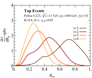
(a)

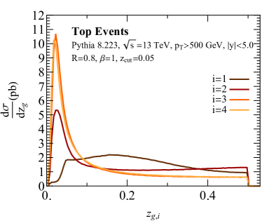
(b)

Figure 3: Distributions in the top jet sample of (a) groomed radius and (b) groomed momentum fraction for $i=1,2,3,4$.

We now consider boosted top quark events from the process $pp\rightarrow t\bar{t}$, forcing the tops to decay in the hadronic channel. In Fig. 3a, we show the $R_{g,i}$ distributions from RSD_i with $i\in\{1,2,3,4\}$, taking $\beta=1$ and $z_{\text{cut}}=0.05$ as baseline parameters. As expected, the groomed radius of the jet decreases as more layers of RSD are applied. There is a small kink structure at lower values of $R_{g}$ for $i=\{1,2\}$ due to the presence of $W$ jets in the top quark decay. In Fig. 3b we show the $z_{g,i}$ distributions, and find that the momentum fraction of the groomed jet is also peaked at values closer to zero as $i$ increases. The sharp cut at 0.5 is because $z_{g}$ is defined as the relative momentum fraction of the softer subjet, which can be at most half. For $i=1$, the $z_{g,i}$ distribution has a nontrivial structure from cases where the clustering history differs from the expected $t\to bW$ topology.

The case of $N=2$ yields a three-pronged grooming strategy, which may be useful for the study of boosted top decays, and we explore this possibility in Sec. 4.5. Alternatively, one can use the $\{R_{g,i},z_{g,i}\}$ values directly to discriminate signal events from backgrounds. For example, we can use ratios like $R_{g,3}/R_{g,2}$ as a probe for boosted top jets, somewhat analogous to the use of the $N$-subjettiness ratio $\tau_{32}$ Thaler:2010tr ; Thaler:2011gf . Similarly, one can use the $z_{g,1}$, and $z_{g,2}$ observables to distinguish QCD-like $1\rightarrow 2$ parton splittings (see e.g. Larkoski:2017bvj ) from hard $t\to bW$ and $W\to q\overline{q}^{\prime}$ decays. In practice, though, top taggers built from $R_{g,i}$ and $z_{g,i}$ do not seem to perform quite as well as $N$-subjettiness (with RSD_∞ grooming), but might remain useful inputs for multivariate analyses, depending on how much $R_{g,i}$ and $z_{g,i}$ are correlated with $N$-subjettiness.

3.2 Non-perturbative effects

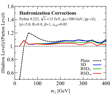
(a)

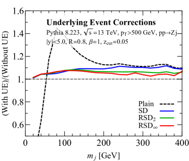
(b)

Figure 4: Study of (a) hadronization and (b) underlying event corrections for different $N$ values, with $\beta=1$ and $z_{\text{cut}}=0.05$. Shown are ratios of the groomed jet mass spectrum as non-perturbative effects are included in Pythia.

Analytical control in jet substructure is mainly limited to perturbative QCD effects. Because internal jet properties probe very exclusive kinematic regions, however, it is not uncommon for non-perturbative effects to yield substantial corrections to perturbative predictions. As such, an important ingredient for robustness of a grooming or tagging algorithm is having a limited sensitivity to non-perturbative contributions, such as hadronization or underlying event. This robustness has already been demonstrated for the mMDT and SD algorithms Dasgupta:2013ihk ; Larkoski:2014wba , and we present here a similar analysis for RSD.

We use the process $pp\to Z+j$ to generate samples of background QCD jets, and use the benchmark RSD parameters $\beta=1$ and $z_{\text{cut}}=0.05$. In Fig. 4a, we plot the ratio of the jet mass distributions before and after the hadronization step in Pythia. Without any grooming, there are around 10% hadronization corrections throughout the whole distribution, with large corrections below a jet mass of $m_{j}\sim 50\,\mathrm{GeV}$. With RSD_N, though, the distribution is significantly more stable down to jet masses of around 20 GeV, independent of the number of RSD layers. Remarkably, in the bulk of the distribution between 50–400 GeV, RSD_∞ exhibits around 5% hadronization corrections. At large mass, the RSD results also show a sizable improvement as one increases the number of RSD layers.

In Fig. 4b, we show the impact of underlying event, plotting the ratio of the jet mass distributions before and after the inclusion of multiple parton interactions (MPI). Here again, we see a similar behavior for all $N>0$ curves in the small mass limit, with relatively small corrections due to non-perturbative underlying event effects. We observe furthermore that as $N\rightarrow\infty$, the stability of the jet mass distributions improves substantially at high masses, such that the overall corrections are less than 10% throughout the distribution. It is therefore clear that RSD with $\beta>0$ substantially improves the robustness of groomed jets to non-perturbative effects, notably by providing more stable results than SD for large jet masses. We also checked that the jet $p_{t}$ was stable to both hadronization and underlying event effects, with similar performance for all $N\geq 1$.

3.3 The $N\rightarrow\infty$ limit of zero-area jets

An interesting property of RSD groomed jets is that their catchment area Cacciari:2008gn goes to zero in the $N\to\infty$ limit. This is due to the fact that soft ghost particles with infinitesimal energy always fail the SD condition in Eq. (2) for $\beta\geq 0$, such that the final jets always have vanishing active and passive areas. For this reason, one might expect that RSD jets would be particularly robust to pileup contamination, a feature we will explore further in Sec. 5. That said, many of the commonly used pileup mitigation techniques, such as the area–median method Cacciari:2007fd ; Cacciari:2008gn , rely in some way on the jet area. Applying these methods to zero-area jets, obtained when grooming with $\text{RSD}_{\infty}$, requires some care (see Sec. 5.2).

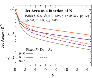
(a)

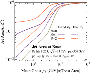
(b)

Figure 5: Jet area studies on quark/gluon jets in $pp\to Zj$ events, for the fixed $R_{0}$ (solid line) and dynamic $R_{0}$ (dashed line) algorithms. (a) Active jet area as a function of the number of soft drop layers $N$. (b) Active jet area as a function of ghost transverse momentum density $\rho$ for RSD_∞.

In Fig. 5a, we use the same $pp\rightarrow Z+j$ samples from Sec. 3.2 and plot the active jet area as a function of the number of RSD layers. Here, we fix $z_{\text{cut}}=0.05$ and scan the exponent $\beta=\{0,1,2\}$, and we explore both the fixed $R_{0}$ and dynamic $R_{0}$ variant from Sec. 2.3. For all choices of $\beta$, the active jet area decreases exponentially with $N$, as anticipated. For smaller $\beta$, the algorithm is more aggressive at removing soft radiation, such that the jet area decreases the most rapidly for $\beta=0$. In Fig. 5a, one can see that the dynamic $R_{0}$ algorithm yields jets with smaller active area for any given $\beta$ value. In this way, dynamic $R_{0}$ behaves more closely to the $\beta=0$ limit of the fixed $R_{0}$ algorithm, leading to decreased pileup sensitivity.

Although RSD_∞ leads to zero-area jets in a formal sense, soft particles from, say, pileup have finite energy in an experimental setting. In Fig. 5b, we plot the effective jet area for $\text{RSD}_{\infty}$ with finite-energy ghost particles, again considering $\beta=\{0,1,2\}$. Here, we report the ghost transverse momentum flow density per unit area, which is roughly 0.5 GeV per $1.0\times 1.0$ bin in rapidity/azimuth for one minimum bias collision. For transverse momentum flow densities starting around 50 GeV—below the pileup $p_{t}$ densities anticipated at the high-luminosity LHC Aad:2015ina —we observe that while the jet area after RSD_∞ grooming is reduced, it remains substantially above zero even in the $N=\infty$ limit. This behavior explains in part why RSD is not sufficient in itself to remove pileup, and instead performs best when combined with another pileup mitigation technique, as discussed in Sec. 5.

4 Improved mass resolution

The simplest way to identify a boosted hadronically-decaying resonance is through the invariant mass of its decay products; in a contamination-free setting, this would correspond to the plain jet mass. In practice, though, the jet mass is particularly sensitive to unassociated soft wide-angle emissions which smears out the distribution. To restore the mass resolution, it is therefore necessary to mitigate soft contamination through appropriate grooming.

While mMDT and SD are not always the most effective methods for enhancing the signal efficiency for boosted objects, they have the advantage of being particularly robust Dasgupta:2016ktv . As seen in Sec. 3.2, hadronization and underlying event effects are suppressed, and they have an analytically-tractable behavior due to the absence of double logarithms and leading non-global contributions Dasgupta:2001sh ; Dasgupta:2002bw ; Dasgupta:2013ihk . To maximize the tagging performance, though, Ref. Butterworth:2008iy found that MDT grooming should be supplemented by an extra filtering step to improve the jet mass resolution. The hope is that an algorithm like RSD_∞ could, by extending the grooming procedure down to smaller angular scales, achieve excellent mass resolution without requiring any further post-processing.

In this section, we study the mass resolution with RSD in three cases of interest for the LHC: 2-prong boosted $W$ bosons, 3-prong boosted top quarks, and 4-prong boosted Higgs jets ($H\to VV\to 4f$). In each case, we use the same Pythia 8.223 generator settings from Sec. 3, and consider all jets in the event that pass the selection cuts $p_{t}>500\,\mathrm{GeV}$ and $|y|<5$. As we will see, RSD provides a way to improve the achievable resolution, with gains in the 10-20% range, while retaining the tractability and robustness of SD.

Our overall recommendation from these studies will be to use RSD_∞ with the default settings of $\beta=1$ and $z_{\text{cut}}=0.05$, which gives good performance across the three test cases. (although other values of $\beta$ and $z_{\text{cut}}$ are worth investigating as well). This conclusion will persist even after the inclusion of pileup in Sec. 5.1, making RSD_∞ useful in extreme environments such as the one faced by the high-luminosity LHC.

4.1 Definition of the mass peak and resolution

To define the mass resolution, we identify the smallest mass interval that contains a fixed fraction $f$ of the total event samples (see e.g. Altheimer:2013yza ). For concreteness, we set $f=0.4$ for these studies. The central value is then defined as the median of the mass interval, and the width is defined as the width of the mass interval.

An alternative approach would be to fit the mass distribution with two curves, a narrow Cauchy distribution to capture the signal and a wider background distribution to account for cases of poor reconstruction. The advantage of the interval method is that it allows us to avoid biases associated with the choice of a fitting functional form. That said, we did test the fitting approach and got similar qualitative features to the ones shown here. We also tested that the choice of fraction $f$ did not affect the qualitative conclusions.

One caveat of the interval method is that it combines two logically distinct effects: mass resolution and signal efficiency. For example, if a technique yields perfect mass resolution, but only on a small subsample of events, then the mass interval will be larger than the resolution in order to include the fixed fraction $f$. In practice, though, many boosted-object taggers select jets based on a fixed mass window, so our definition of mass resolution is appropriate for that setting.

4.2 Two-prong $W$ decays

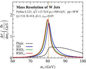
(a)

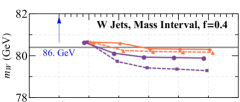
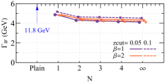
(b)

Figure 6: (a) Mass distributions for the $W$ jet sample using different levels of RSD and the benchmark values of $\beta=1$ and $z_{\text{cut}}=0.05$. (b) Central mass values and widths as a function of $N$, testing four different $\beta$ and $z_{\text{cut}}$ combinations, using a mass interval containing a fraction $f=0.4$ of the events.

In Fig. 6a, we show the jet mass distribution from a $W$ jet sample obtained from $pp\to WW$, with the $W$ decaying hadronically. At least some level of grooming is required to obtain a peak within $10\%$ of the $W$ mass. With $\beta=1$ and $z_{\text{cut}}=0.05$, the jet mass distribution is already close to the expected $W$ mass value after applying SD alone. Adding additional SD layers with $N\geq 2$, the peak shifts somewhat below the expected $W$ mass value, but, more importantly, the width of the mass distribution decreases. Another interesting observation is that the mass distribution is more symmetric with additional grooming layers, such that with $N=\infty$, the jet mass can be accurately fit by a Cauchy distribution.

To get a sense of the dependence on the choice of RSD parameters, in Fig. 6b we plot the central value and width of the mass distribution as a function of $N$. As discussed in Sec. 4.1, we use a mass interval containing a fraction $f=0.4$ of events. The benchmark parameters of $\beta=1$ and $z_{\text{cut}}=0.05$ undershoot the $W$ mass central value by around 1 GeV, while switching to $\beta=2$ gives a better reconstruction of the central value. On the other hand, the benchmark parameters yield the best $W$ mass resolution, which implies somewhat better tagging performance. More generally, all of the RSD settings yield a sizable improvement over the ungroomed case and a smaller but clearly visible improvement, of order 10–20%, over the SD case in terms of resolution.

4.3 Three-prong top decays

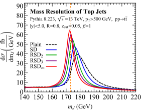
(a)

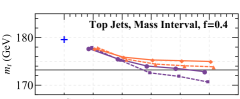
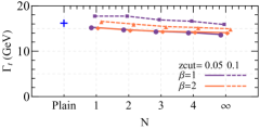
(b)

Figure 7: Same as Fig. 6 but for the top jet sample.

Unlike SD, which terminates after probing only the leading two subjets, RSD with $N>1$ is well suited to handle the broad radiation patterns and three-prong topologies of top quarks. We consider a sample of $pp\rightarrow t\overline{t}$ events, where the top mass in Pythia is set to 173.2 GeV. In Fig. 7a, we show the mass distribution of boosted tops for different layers of RSD. As expected, we find that without grooming, the peak of the distribution occurs at values well above the top mass. With successive layers of RSD grooming, the mass peak shifts to lower values, and converges very close to the top mass for $N=\infty$. This is due to the fact that we discard more of the extra unassociated radiation, and therefore the mass tends to decrease.

In Fig. 7b, we consider the central mass value and width containing a fraction $f=0.4$ of the mass distribution. We find that $\beta=1$ and $z_{\rm{cut}}=0.05$ gives nearly optimal performance (by the mass interval measure), with $\beta=2$ and $z_{\rm{cut}}=0.1$ giving comparable performance in terms of accuracy and resolution. The gain in resolution compared to SD is found to be slightly larger than 10%.

Compared to the $W$ case in Sec. 4.2, where the resolution tends to saturate by $N=2$, the top case benefits from taking $N\geq 3$. In fact, there is a marginal benefit from taking $N\to\infty$, which is why we recommend RSD_∞ for mass resolution studies involving the top quark. It would be interesting to see whether RSD_∞ would also be appropriate for defining a short-distance top quark mass Hoang:2017kmk .

4.4 Four-prong Higgs decays in associated production

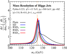
(a)

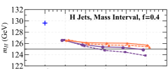
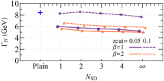
(b)

Figure 8: Same as Fig. 6 but for the Higgs jet sample.

Four-prong jets can provide important information in certain Higgs decays, where the $H\rightarrow VV\rightarrow 4f$ channel plays an important role in determining properties of the Higgs Choi:2002jk as well as its couplings to bosons Meyer:2004ha . They can also provide a useful probe for new physics, such as in hadronic decays of heavy resonances decaying to $HW$ or $HZ$ Khachatryan:2015bma , or in hadronic decays of a boosted Higgs pair Bishara:2016kjn .

In Fig. 8a, we show the reconstructed Higgs mass in boosted $H\rightarrow W^{+}W^{-}\rightarrow q\bar{q}q\bar{q}$ decays. This comes from a sample of $pp\rightarrow HZ$ events, with the $Z$ boson decaying to neutrinos. Although grooming with ordinary SD performs relatively well, the Higgs mass reconstruction is better with $N\geq 3$, as one would expect for a four-particle decay. A comparison of the central mass values and width for different grooming parameters is shown in Fig. 8b, showing gains in resolution around 10–15%. Once again, the benchmark choice of $\beta=1$ and $z_{\rm{cut}}=0.05$ gives an excellent reconstruction, especially in the $N\to\infty$ limit, although $\beta=2$ and $z_{\rm{cut}}=0.05$ gives a slightly better resolution.

4.5 Boosted top tagging

We conclude this section with a concrete example of the impact of improved mass resolution from RSD. Using the same samples as Sec. 4.3, we perform a study of boosted top tagging performance. We consider two standard observables used for discriminating top jets from QCD background: the $N$-subjettiness ratio $\tau_{32}=\tau_{3}/\tau_{2}$ Thaler:2010tr ; Thaler:2011gf , and the generalized energy correlation function ratio $N_{3}^{(2)}={}_{2}e^{(2)}_{4}/({}_{1}e^{(2)}_{3})^{2}$ Larkoski:2013eya ; Moult:2016cvt . By adjusting the degree of grooming—on both the jet mass and on the jet discriminant—we can assess the potential performance gains from RSD.

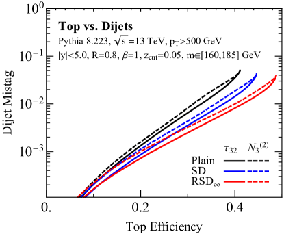
Figure 9: Top jet signal efficiency versus dijet background mistag rate, with the benchmark RSD parameters of $\beta=1$ and $z_{\text{cut}}=0.05$.

In Fig. 9, we plot the top signal efficiency versus dijet background mistag rate (ROC curves). The rightmost endpoints of the ROC curve indicate the impact of an overall cut of $m_{\text{groomed}}\in[160,185]$. As $N$ increases, the dijet mistag rate improves somewhat, and the top signal efficiency increases due to the improved mass resolution. The rest of the ROC curve is associated with sweeping a cut on $\tau_{32}$ and $N_{3}$. Note that as the substructure cut becomes more stringent, there is less of a gain from increasing the number of grooming layers. The reason is that grooming removes part of the radiation phase-space where there is still some discriminating power, or equivalently, a cut on $\tau_{32}$ or $N_{3}$ already removes some of the phase-space regions targeted by grooming. Because this phase-space region is also the most sensitive to non-perturbative effects, there is a tradeoff between tagging performance and non-perturbative robustness Dasgupta:2016ktv . Despite this tradeoff, RSD_∞ maintains the best tagging performance for top efficiencies greater than 10%.

As discussed in Ref. Moult:2016cvt , $\tau_{32}$ with grooming and $N_{3}$ with grooming have the same soft-collinear power counting, so their performance is expected to be similar (see further discussion in Ref. Larkoski:2014gra ). This conclusion persists even with multiple grooming layers. The relative difference between $\tau_{32}$ and $N_{3}$ then depends on the precise details of the event selection. $N_{3}$ is not defined with respect to any axes, so it is expected to perform better than $\tau_{32}$ in kinematic regimes where the choice of axes can be ambiguous Moult:2016cvt . Here, though, we are taking a rather tight mass window of $m_{\rm jet}\in[160,185]$ GeV, so the axes effects are subleading and $\tau_{32}$ turns out to give better performance. Though not shown, we also tested the performance of the $M_{3}$ observable Moult:2016cvt . While $M_{3}$ always performs worse than $\tau_{32}$ or $N_{3}$, the relative improvement in going from SD to RSD_∞ is greater due to the removal of radiation in all three prongs.

We found similar tagging results for other boosted objects, such as hadronic decays of boosted $W$ and Higgs bosons. In general, RSD_∞ gives similar or improved performance compared to tagging with SD, though most of that comes just from the improved mass resolution. For the case of $W$ tagging, it would be interesting to study a version of the dichroic $N$-subjettiness ratio Salam:2016yht , where RSD_∞ is used to compute the jet mass and $\tau_{1}$ (or ${}_{1}e_{2}$), and a lighter grooming, like (R)SD with larger $\beta$ and smaller $z_{\text{cut}}$, is used to calculate $\tau_{2}$ (or ${}_{2}e_{3}$). Results for boosted top tagging with large pileup multiplicity are shown in App. B.2.

5 Robust pileup mitigation

As the LHC progresses towards ever higher luminosities, mitigating the effect of secondary proton-proton collisions becomes an increasingly important challenge. Large pileup levels can substantially impact typical jet observables, increasing for example the jet’s momentum, while shifting and distorting jet shapes. A number of techniques have been developed to remove soft radiation associated with secondary vertices. These include area–median Cacciari:2007fd ; Cacciari:2008gn or shape Soyez:2012hv subtraction; grooming with trimming Krohn:2009th , pruning Ellis:2009me , or mMDT/SD Dasgupta:2013ihk ; Larkoski:2014wba ; charged hadron subtraction CMS:2009nxa ; particle-level removal methods such as SoftKiller Cacciari:2014gra and PUPPI Bertolini:2014bba ; and machine learning methods Komiske:2017ubm . In practice, in the context of jet substructure, it is generally most useful to combine a removal or subtraction method with some type of jet grooming to achieve optimal results (see e.g. Altheimer:2013yza ).

Here, we investigate the properties of jets after grooming with RSD under varying levels of pileup, with additional pileup studies appearing in App. B. We will see that, when used in combination with SoftKiller Cacciari:2014gra , the RSD algorithm yields robust pileup mitigation results even under high pileup conditions. We will also test RSD with the area–median subtraction approach Cacciari:2007fd .

5.1 Mass resolution with SoftKiller

SoftKiller is an event-wide particle-level removal method, which uses a dynamic cut on transverse momentum $p_{t}^{\text{cut}}$ to remove soft particles Cacciari:2014gra . The threshold is determined dynamically on an event-by-event basis as follows:

1. The event is split into patches of size $a_{\rm SK}\times a_{\rm SK}$ in rapidity-azimuth space.

2. For each patch, one determines $p_{t,i}^{\text{max}}$, the largest particle transverse momentum in patch $i$.

3. The transverse momentum threshold $p_{t}^{\text{cut}}$ is determined by

   $$p_{t}^{\text{cut}}=\underset{i}{\text{median}}\,\left(p_{t,i}^{\text{max}}\right)\,,$$ (3)

   where the median is taken across all patches.

4. All particles with transverse momenta below $p_{t}^{\text{cut}}$ are removed from the event.

An equivalent description of SoftKiller is finding the minimal $p_{t}^{\text{cut}}$ such that exactly half of the patches have zero momenta. This $p_{t}^{\text{cut}}$ ensures that the median across patches of transverse-momentum flow per unit area $\rho$ is zero.

For each analysis, one has to set the appropriate patch size by choosing the SoftKiller parameter $a_{\rm SK}$. The goal is to set the parameter $a_{\rm SK}$ to minimize both the shift in jet $p_{t}$ and mass. After RSD grooming of $R=0.8$ jets, this usually achieved with $a_{\rm SK}=0.5$, although this was found to be somewhat process dependent. For the case of $pp\rightarrow t\bar{t}$, the dependence of the jet mass on the choice of grid parameter is shown in Fig. 10. We find that the position of the top peak depends significantly on the value of $a_{\rm SK}$ with small (large) values of $a_{\text{SK}}$ showing a clear undersubtraction (oversubtraction). In our simulations, $a_{\rm SK}\simeq 0.5$ shows only a small average bias, so we take this value as our benchmark.

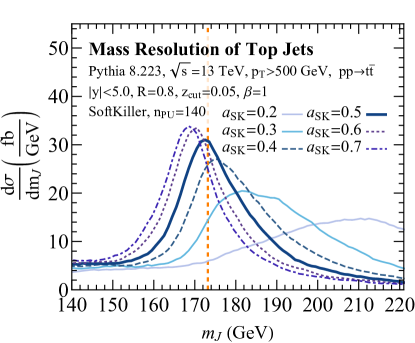
Figure 10: The RSD groomed mass distribution for multiple values of the SK grid parameter $a_{\rm SK}$.

We now study the effects of pileup on the mass resolution in groomed jets, following the same analysis strategy as Sec. 4. Since the behavior is quite similar to that observed previously, we focus here only on top events, with the $W$ and Higgs cases discussed in App. B.1.

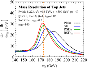
(a)

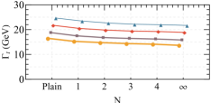
(b)

Figure 11: (a) Same as Fig. 7a, but with 140 pileup vertices and using a SoftKiller parameter of $a_{\rm SK}=0.5$. (b) Central mass values and widths as a function of $N$ for several pileup multiplicities, using the benchmark RSD/SoftKiller parameters and $f=0.4$.

We use the same $pp\to t\bar{t}$ process as in Sec. 4.3, with the Pythia top mass at 173.2 GeV. In Fig. 11a, we show the top jet mass distribution with the addition of 140 pileup vertices. With SoftKiller but without any jet grooming, there is a 12 GeV shift in the reconstructed top mass peak. (The shift would be larger than 200 GeV if SoftKiller were not applied.) The shift decreases to about 5 GeV after applying SD, with additional improvements in going to RSD₂ and RSD_∞. Though the shape of the top mass distribution is not nearly as symmetric as without pileup, RSD_∞ does restore some of the symmetry of the top mass distribution compared to SoftKiller alone.

In Fig. 11b, we show the central mass value and width after the application of SoftKiller and RSD_N for several pileup levels. As $n_{\text{PU}}$ increases from 0 to 140, the central top mass value and the width increases monotonically, even with the application of SoftKiller. By applying more layers of RSD, the central top mass decreases toward the physical value, with somewhat improved stability across the different pileup levels. The best performance is obtained for RSD_∞, in agreement with the analysis of Sec. 4.3, and the mass difference is less than 5 GeV even at the highest pileup level. This shows that, as well as improving the resolution of observables such as the jet mass, grooming with RSD somewhat improves the stability of the distributions as a function of the number of pileup vertices $n_{\text{PU}}$. That said, there are still substantial distortions to the width of the top mass distribution even after RSD_∞, reflecting the underlying challenge of pileup at the LHC.

5.2 Mass resolution with the area–median method

Let us now consider pileup mitigation using RSD in conjunction with the area–median method Cacciari:2007fd ; Cacciari:2008gn . This removal technique is widely used in experimental analyses, and we therefore provide a short study of its use with RSD groomed jets.

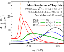
(a)

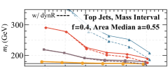
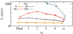
(b)

Figure 12: (a) Similar to Fig. 11a, but with 60 pileup vertices and using an area–median parameter of $a=0.55$. Note the larger mass range shown and the inclusion of both fixed-$R_{0}$ and dynamic-$R_{0}$ results. (b) Same as Fig. 11b but for the area–median method applied to RSD with dynamic $R_{0}$.

Generally speaking, combining the area–median procedure with grooming requires more than just subtracting the jet after grooming. Indeed, since the grooming procedure imposes kinematic constraints on subjets, one wants to apply the subtraction procedure directly on the subjets, so that these kinematic constraints use quantities which have been corrected for pileup (see e.g. Altheimer:2013yza ). In the case of RSD (and mMDT/SD), this means that, at each step of the declustering procedure, we should apply an area–median subtraction to both subjets before imposing the SD condition in Eq. (2). Note that even in the case of RSD_∞ where the final groomed jet has zero area, intermediate subjets have a non-zero area, so subtracting the intermediate subjets is crucial.

The resulting mass peak is shown in Fig. 12a, for both a dynamic and fixed $R_{0}$ implementation of RSD for 60 pileup events, using the area–median parameter $a=0.55$. We find that only the most aggressive algorithm RSD_∞, preferably using dynamic $R_{0}$ from Sec. 2.3, succeeds at reconstructing the top peak. This is confirmed by Fig. 12b, where we show the central mass values and widths for various pileup levels. Despite the fact that RSD_∞ with dynamic $R_{0}$ does recover the top mass peak, one should still note that the mass resolution (and median peak position) significantly worsens with increasing pileup multiplicity, encouraging the investigation of more recent particle-level pileup mitigation techniques for future runs of the LHC.

6 Bottom-Up Soft Drop for event-wide grooming

We have seen that the default RSD algorithm in Sec. 2.2 yields sensible grooming behaviors across a wide range of applications, with excellent overall performance for $N=\infty$. It is possible, however, to obtain similar results with a different approach. In this section, we introduce an alternative to RSD_∞ called Bottom-Up Soft Drop (BUSD), which is also available in RecursiveTools ($\geq$2.0.0) through fastjet-contrib fjcontrib .

The default RSD is a top-down algorithm, where the SD condition in Eq. (2) is imposed by declustering a jet starting from its clustering tree. By contrast, BUSD imposes Eq. (2) as part of a (re)clustering procedure, effectively starting from the leaves of the clustering tree. BUSD can either be applied to a single jet (local BUSD) or to the event as a whole (global BUSD).

With either BUSD approach, the SD criteria is applied at each pairwise combination during the reclustering stage, somewhat like pruning Ellis:2009me . In the fastjet-contrib implementation, this is achieved through a modified recombination scheme, such that at each step of the reclustering with a large-$R$ C/A algorithm, the pseudojet obtained from combining particles $i$ and $j$ with smallest distance $d_{ij}=\Delta R_{ij}/R_{0}$ is given by

$$p_{ij}=\left\{\begin{array}[]{ll}\max(p_{i},p_{j})&\mbox{if Eq.~{}(\ref{eq:SD-crit}) fails,}\\ p_{i}+p_{j}&\mbox{otherwise,}\end{array}\right.$$ (4)

where the maximum is defined by $p_{t}$. In the definition of $d_{ij}$, we choose $R_{0}$ to match the SD criteria in Eq. (2). For the studies below, we always match the parameter $R_{0}$ to the jet radius $R$.

With local BUSD, the reclustering is applied to an individual jet found by another jet algorithm. While one cannot obtain finite $N$ results with BUSD, the bottom-up algorithm provides results that are very similar to the $N=\infty$ top-down approach of $\text{RSD}_{\infty}$. This is expected, since local BUSD uses the same initial jet constituents as $\text{RSD}_{\infty}$.

With global BUSD, the full event is clustered into a single large C/A tree. This provides an event-wide grooming strategy that does not require any specific jet definition. After grooming with global BUSD, the groomed event contains only a subset of the initial particles, so any jet definition can be used to cluster the remaining particles. The resulting jets are guaranteed to have zero active area, without any additional treatment required for each individual jet.

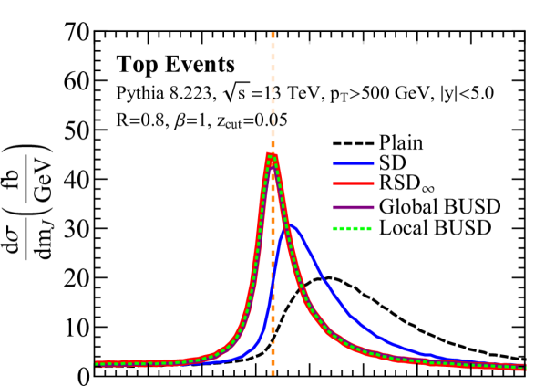
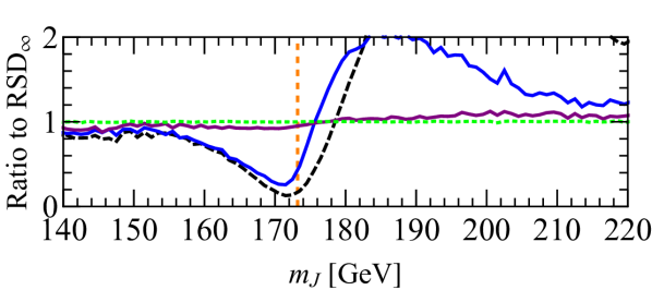
(a)

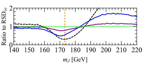
(b)

Figure 13: Behavior of global and local BUSD on $t\bar{t}$ events with the default RSD parameters. (a) Performance without pileup, to be compared to Fig. 7a. (b) Performance with 140 pileup vertices plus SoftKiller, to be compared to Fig. 11a. In both panels, the ratios to RSD_∞ are shown at the bottom.

The behavior of BUSD is shown in Fig. 13a for the same $pp\to t\bar{t}$ sample from Sec. 4.3. Without pileup, $\text{RSD}_{\infty}$, local BUSD, and global BUSD give nearly identical results on the top jet mass distribution. This suggests that globally grooming an event before the jet clustering stage could be a practical alternative to standard jet-based grooming.

We test the robustness of BUSD to pileup in Fig. 13b. As in Sec. 5.1, we overlay 140 pileup vertices and apply the SoftKiller algorithm with grid parameter $a_{\rm SK}=0.5$. There is still nearly identical behavior for $\text{RSD}_{\infty}$ and local BUSD, with somewhat degraded performance seen using global BUSD. So while global BUSD grooming still performs better than the original SD in reconstructing the top mass, it is outperformed by $\text{RSD}_{\infty}$ (and local BUSD) in extreme environments.

7 Conclusions

Recursive Soft Drop (RSD) is a generalization of the original mMDT/SD algorithm, which has already seen successful applications at the LHC. By recursively applying the SD declustering procedure $N$ times, RSD_N can remove jet contamination more efficiently and with looser SD parameters than original SD. With benchmark parameters $\beta=1$ and $z_{\text{cut}}=0.05$, we found that RSD grooming performs particularly well in the fully-recursive $N=\infty$ limit. This limit also shows an improved robustness against pileup effects, a feature which is likely connected to the fact that RSD_∞ yields groomed jets with formally zero area.

Jet grooming with RSD provides several refinements over previous techniques, notably by increasing the robustness to non-perturbative effects and by improving the mass resolution for boosted heavy resonances such as $W$ bosons, top quarks, and Higgs bosons. In the context of jet tagging, the additional declustering layers have a modest impact on QCD backgrounds, so much of the gains in tagging performance come from the improved jet mass resolution. While RSD_N-1 seems to be the natural choice for grooming $N$-prong objects, we have noticed that adding more grooming layers, e.g. using RSD_N, comes with further resolution gains. In the end, we recommend the use of RSD_∞, since it offers the same or better performance in our case studies with no discernible downsides. The one possible exception is for boosted $W$ bosons, where RSD_∞ gave a better $W$ boson resolution compared to SD but at the expense of shifting the $W$ peak location by ${\cal{O}}(1)$ GeV. That said, this shift could be minimized by using lower values of $z_{\text{cut}}$ or higher values of $\beta$.

For pileup mitigation, RSD works best when paired with a particle-level removal algorithm such as SoftKiller. In the presence of pileup, we found substantial improvements in the groomed mass resolution after grooming with RSD when compared to the original SD procedure. We recommend the use of RSD_∞ in high luminosity environments, since this always performed better than RSD with finite $N$. It is also possible to use RSD with area-based pileup subtraction methods, as long as the corrections are applied on the finite-area subjets that enter into the SD condition.

An interesting alternative to RSD_∞ is Bottom-Up Soft Drop (BUSD). In its local variant, i.e. applied to a single jet, it shows similar performance to RSD_∞, with comparable resilience to pileup effects. BUSD also admits a global implementation, where it is applied at the event-wide level to groom an event without committing to a particular jet algorithm. This latter variant shows, however, a slightly larger sensitivity to pileup than RSD_∞.

Since RSD is closely related to the mMDT/SD algorithms, it shares the advantage of retaining analytic tractability. We look forward to future studies aimed at high-precision and systematically-improvable analytical results of tagging rates. These could be achieved with existing frameworks to leading-logarithmic accuracy, and could potentially be extended to higher logarithmic accuracy through a suitable extension of the CAESAR Banfi:2004yd and ARES Banfi:2014sua ; Banfi:2016zlc methods or through a modified factorization theorem Frye:2016okc in soft-collinear effective theory Bauer:2000yr ; Bauer:2001ct ; Bauer:2001yt ; Bauer:2002nz . An interesting potential application of RSD is in defining the short-distance top quark mass using light grooming Hoang:2017kmk .

Finally, RSD could also find useful applications in the context of heavy ion collisions, where jet grooming can provide a powerful probe into the effects of the medium on the momentum sharing $z_{g}$ Sirunyan:2017bsd ; Chien:2016led ; Mehtar-Tani:2016aco ; Milhano:2017nzm . By adjusting the number of grooming layers $N$, one can achieve a more aggressive grooming while retaining more of the underlying hard scattering process. Furthermore, the groomed energy fractions $z_{g,i}$ obtained at every SD layer $i$ may provide an additional handle to study the propagation of partons through the quark-gluon plasma at multiple resolution scales.

Appendix A Behavior at fixed order

In this appendix, we study the behavior of RSD at fixed order in $\alpha_{s}$. To this end, we use Event2 Catani:1996jh ; Catani:1996vz to produce a sample of boosted heavy bosons decaying (at tree level) to a quark-antiquark pair. We start from an $e^{+}e^{-}$ collision at a given center-of-mass energy $M\equiv\sqrt{s}$, corresponding to the mass of the heavy boson. Then, we boost the partonic system transversely such that the heavy boson is traveling along the $x$ axis of the collision with transverse momentum $p_{t}$. In what follows, we fix $M=100$ GeV and $p_{t}=500$ GeV. We cluster the event with the anti-$k_{t}$ algorithm with $R=0.8$, and we apply RSD_N with $\beta=1$, $z_{\text{cut}}=0.2$, varying the number of layers $N$. Note the use of a larger $z_{\text{cut}}$ value compared to our recommended default to make the impact of RSD more visible.

The motivation for studying such boosted systems is that it provides a source of jets with 2, 3, and 4 partons at respective orders $\alpha_{s}^{0}$, $\alpha_{s}^{1}$, and $\alpha_{s}^{2}$, allowing us to study the effects of several layers of RSD.

Let us start by discussing the jet mass in Fig. 14a. Instead of plotting the mass distribution after applying RSD_N, we plot the difference

$$\Delta\sigma_{N}(m)=\frac{1}{\sigma_{\text{Born}}}\left[\left.\frac{d\sigma}{dm}\right|_{\text{RSD}_{N+1}}-\left.\frac{d\sigma}{dm}\right|_{\text{RSD}_{N}}\right],$$ (5)

i.e. the difference in the mass spectrum between two consecutive layers of RSD. From top to bottom, Fig. 14a shows $\Delta\sigma_{N}$ for tree-level events ($e^{+}e^{-}\to q\bar{q}$) at ${\cal{O}}(\alpha_{s}^{0})$, the order $\alpha_{s}$ correction, and the order $\alpha_{s}^{2}$ correction.

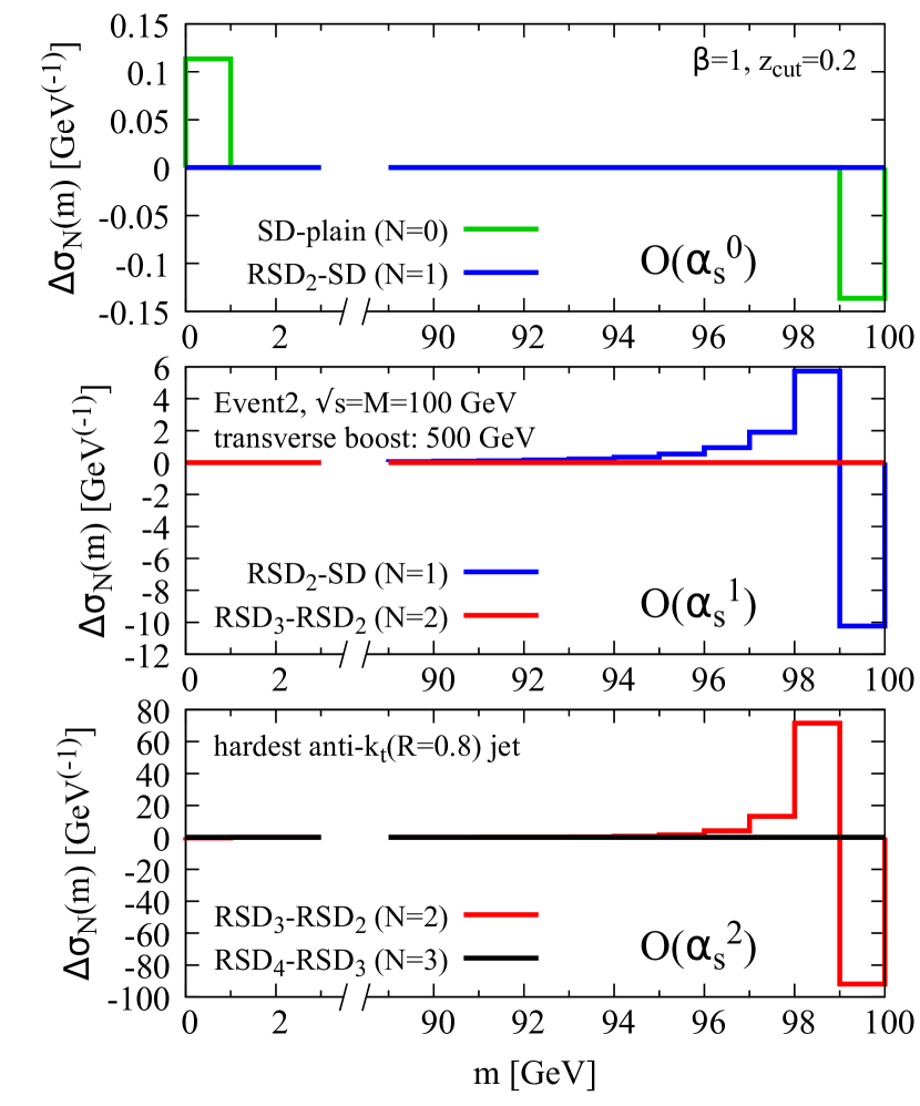
(a)

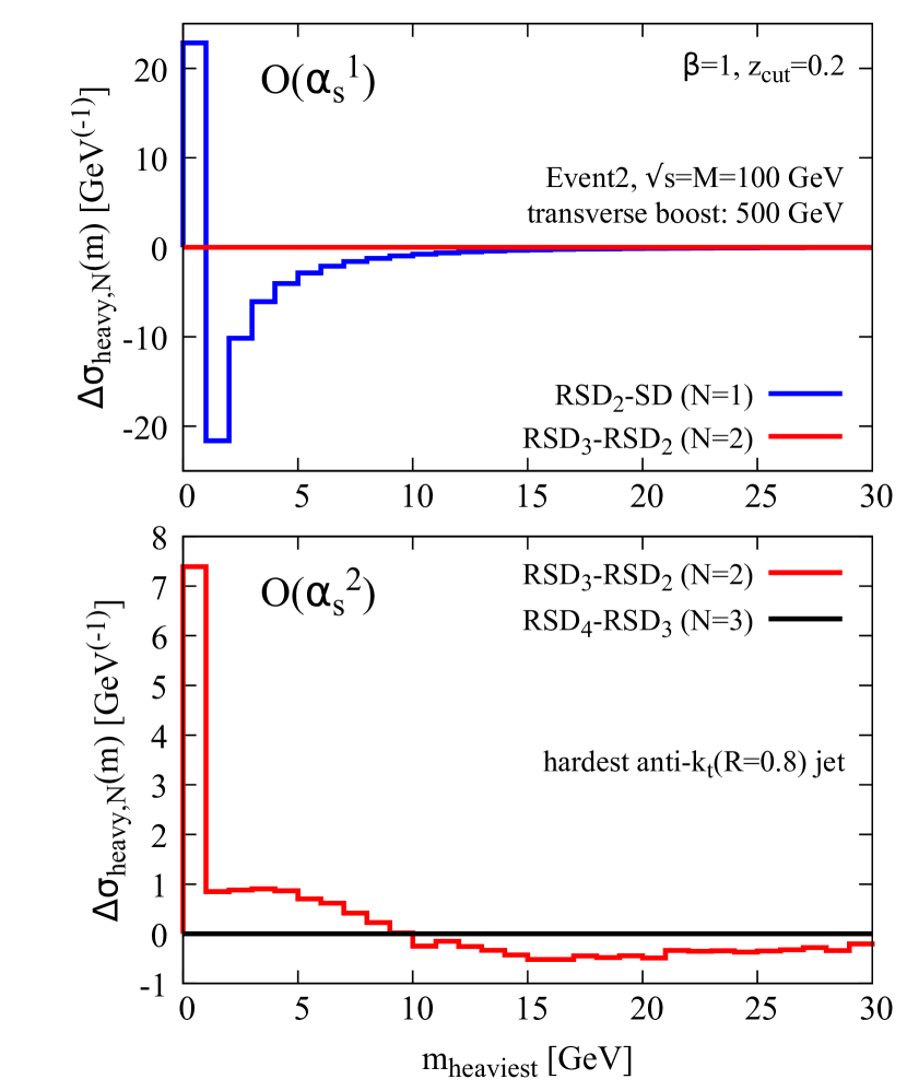
(b)

Figure 14: Fixed-order coefficients from Event2 for (a) the jet mass distribution and (b) the heavier subjet mass distribution. The plot shows Eq. (5), the difference in the jet mass spectrum obtained with consecutive layers of RSD.

At ${\cal{O}}(\alpha_{s}^{0})$, there is either one or two partons in the jet. For one parton, the jet mass is always zero, irrespectively of the number of layers of RSD. Jets with two partons, however, have a (plain) jet mass $M$. Therefore, if we apply SD = RSD₁ to such a jet, we can either have a jet with two partons and a mass $M$, or a jet with one parton and a zero mass, depending on whether or not the SD condition is satisified. Since there is no additional substructure to probe in the jet, applying additional SD layers with RSD_N>1 will not have any effect. This expectation is indeed observed in the top panel of Fig. 14a: applying the first layer of SD yields a decrease of the cross section for $m=M=100$ GeV and an increase at zero mass, i.e. $\Delta\sigma_{0}\neq 0$, and additional SD layers have no effect, i.e. $\Delta\sigma_{(\geq)1}=0$.

At order $\alpha_{s}$, we now have jets with three partons, which is enough to see a non-trivial effect from RSD₂. Indeed, if we have a jet with three partons for which the first declustering passes the SD condition, the second SD layer will sometimes be applied on a subjet itself made of two partons; if this system fails the SD condition, the RSD₂ mass will be smaller than the RSD₁ mass, with all subsequent layers being ineffective. This is seen in the middle panel of Fig. 14a, with $\Delta\sigma_{1}$ showing a shift towards smaller masses and $\Delta\sigma_{(\geq)2}=0$.

Unsurprisingly, the same pattern is observed at order $\alpha_{s}^{2}$, just one layer further down, with $\Delta\sigma_{2}$ showing a decrease in mass while $\Delta\sigma_{{\geq}3}=0$. Note that although the two-loop virtual corrections, contributing at ${\cal{O}}(\alpha_{s}^{2})$, are not available in Event2, they correspond to events where the jets can have at most two partons and so do not contribute to $\Delta\sigma_{N\geq 1}$. Ultimately, we see that each successive SD layer further grooms the jet. For the $N^{\text{th}}$ layer of SD to be effective, one needs at least $N+1$ partons in the jet, hence $\Delta\sigma_{N}$ being non-zero starting at order $\alpha_{s}^{N}$.

In addition to the jet mass distribution, we can also study the mass spectrum of the heavier subjet in a jet, shown in Fig. 14b. This is defined by applying RSD to the jet and taking, in the resulting groomed jet, the heavier of the two subjets corresponding to the first declustering that has passed the SD condition. Taking the example of Fig. 2, this is the heavier of the RSD subjets tagged at vertex “1”, i.e. the heavier of the subjet made of the two upper kept particles and the subjet made of the two lower kept particles.

At ${\cal O}(\alpha_{s}^{0})$, there can be at most one particle in a subjet so the heavier subjet mass is always 0. At higher orders, though, one can get more partons and hence a non-zero subjet mass. We study the difference $\Delta\sigma_{\text{heavy},N}(m)$ in Fig. 14b, defined analogously to Eq. (5) as the difference in the heavier subjet mass distribution between $N$ and $N+1$ layers of RSD. As with the jet mass, we need at least $N+2$ partons in the jet to get a non-zero $\Delta\sigma_{\text{heavy},N}$, a situation which starts at order $\alpha_{s}^{N}$. This is confirmed by our Event2 simulations where, for example, $\Delta\sigma_{\text{heavy},1}$ is already different from zero at ${\cal O}(\alpha_{s})$ while $\Delta\sigma_{\text{heavy},2}$ starts being non-zero at ${\cal O}(\alpha_{s}^{2})$.

A calculation of the logarithmically-enhanced terms appearing in these distributions could serve as a base for an analytic study of RSD.

Appendix B Additional pileup studies

In this appendix, we present additional results for RSD in high pileup conditions.

B.1 $W$ and Higgs mass resolution with SoftKiller

Analogously to the case of 3-pronged top decays in Sec. 5.1, here we show results for 2-prong boosted $W$ bosons and 4-prong boosted $H$ bosons. In all cases, we use the default RSD parameters $\beta=1$ and $z_{\text{cut}}=0.05$, and apply SoftKiller with $a_{\rm SK}=0.5$.

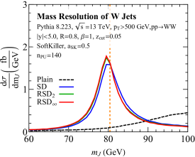
(a)

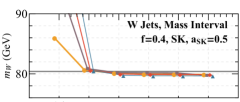
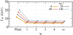
(b)

Figure 15: Same as Fig. 11 but for the $W$ boson sample.

The $W$ mass distribution is shown in Fig. 15a, with the addition of 140 pileup vertices. This is using the same event samples as in Sec. 4.2 and can be compared to Fig. 7a. Already, the performance is very good for SD alone, though the mass resolution is improved somewhat going to RSD₂ or RSD_∞. Note that the distribution becomes a bit more symmetric, though not nearly as much as in the case without pileup. In Fig. 15b, we show the central mass value and width as a function of number of SD layers for different pileup levels. One can see that as $N$ increases, the peak location improves while the distribution becomes narrower, though the performance basically saturates at $N=2$.

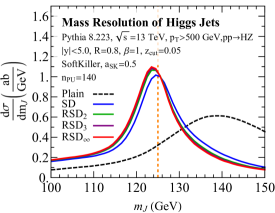
(a)

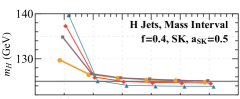
(b)

Figure 16: Same as Fig. 11 but for the $H(\rightarrow 4q)$ boson sample.

In Fig. 16a we show the mass distribution for $H\rightarrow 4q$ decays, again with 140 pileup vertices. This is using the same event samples as in Sec. 4.4 and can be compared to Fig. 8a. Again, one can observe a small improvement in both the location of the central value and the width of the distribution as the number of SD layers is increased. This is shown more explicitly in Fig. 16b, where we can see the narrowing of the distribution and convergence of the peak for different pileup levels, with performance saturating around $N=3$ or $N=4$.

B.2 Boosted top tagging with pileup

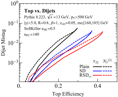
Figure 17: Same as Fig. 9, but with 140 pileup vertices and SoftKiller with grid parameter $a_{\rm SK}=0.5$.

Here, we repeat the top tagging study in Sec. 4.5 in the presence of pileup, again using SoftKiller with a grid parameter $a_{\rm SK}=0.5$. In Fig. 17, we show the same ROC curve as in Fig. 9, but with the addition of 140 pileup vertices. As in the previous study without pileup, additional SD grooming layers improve the signal efficiency, with the observables after RSD leading to much better discrimination between top and QCD jets. Here, though, the improvement is much more substantial, since the gains in mass resolution in high-pileup condition is quite dramatic; see Sec. 5.1. This allows for reasonable top tagging performance even with a narrow $m\in[160,185]\,\mathrm{GeV}$ top window, despite the large pileup multiplicity.

References

- (1) A. Abdesselam et al., Boosted objects: A Probe of beyond the Standard Model physics, Eur. Phys. J. C71 (2011) 1661, [arXiv:1012.5412].
- (2) A. Altheimer et al., Jet Substructure at the Tevatron and LHC: New results, new tools, new benchmarks, J. Phys. G39 (2012) 063001, [arXiv:1201.0008].
- (3) A. Altheimer et al., Boosted objects and jet substructure at the LHC. Report of BOOST2012, held at IFIC Valencia, 23rd-27th of July 2012, Eur. Phys. J. C74 (2014), no. 3 2792, [arXiv:1311.2708].
- (4) D. Adams et al., Towards an Understanding of the Correlations in Jet Substructure, Eur. Phys. J. C75 (2015), no. 9 409, [arXiv:1504.00679].
- (5) M. Cacciari, Phenomenological and theoretical developments in jet physics at the LHC, Int. J. Mod. Phys. A30 (2015), no. 31 1546001, [arXiv:1509.02272].
- (6) A. J. Larkoski, I. Moult, and B. Nachman, Jet Substructure at the Large Hadron Collider: A Review of Recent Advances in Theory and Machine Learning, arXiv:1709.04464.
- (7) D. Bhatia, R. Camacho, G. Chachamis, S. Chatterjee, F. Dreyer, D. Kar, P. Loch, I. Moult, B. Nachman, A. Papaefstathiou, T. Samui, A. Siodmok, G. Soyez, and J. Thaler, Performance versus robustness: Two-prong substructure taggers for the LHC, contribution to the Les Houches 2017: Physics at TeV Colliders Standard Model Working Group Report, 2018. arXiv:1803.07977.
- (8) M. H. Seymour, Tagging a heavy Higgs boson, in ECFA Large Hadron Collider Workshop, Aachen, Germany, 4-9 Oct 1990: Proceedings.2., pp. 557–569, 1991.
- (9) M. H. Seymour, Searches for new particles using cone and cluster jet algorithms: A Comparative study, Z. Phys. C62 (1994) 127–138.
- (10) J. M. Butterworth, B. E. Cox, and J. R. Forshaw, scattering at the CERN LHC, Phys. Rev. D65 (2002) 096014, [hep-ph/0201098].
- (11) J. M. Butterworth, J. R. Ellis, and A. R. Raklev, Reconstructing sparticle mass spectra using hadronic decays, JHEP 05 (2007) 033, [hep-ph/0702150].
- (12) J. M. Butterworth, A. R. Davison, M. Rubin, and G. P. Salam, Jet substructure as a new Higgs search channel at the LHC, Phys. Rev. Lett. 100 (2008) 242001, [arXiv:0802.2470].
- (13) J. Thaler and L.-T. Wang, Strategies to Identify Boosted Tops, JHEP 07 (2008) 092, [arXiv:0806.0023].
- (14) D. E. Kaplan, K. Rehermann, M. D. Schwartz, and B. Tweedie, Top Tagging: A Method for Identifying Boosted Hadronically Decaying Top Quarks, Phys. Rev. Lett. 101 (2008) 142001, [arXiv:0806.0848].
- (15) D. Krohn, J. Thaler, and L.-T. Wang, Jet Trimming, JHEP 02 (2010) 084, [arXiv:0912.1342].
- (16) S. D. Ellis, C. K. Vermilion, and J. R. Walsh, Techniques for improved heavy particle searches with jet substructure, Phys. Rev. D80 (2009) 051501, [arXiv:0903.5081].
- (17) S. D. Ellis, C. K. Vermilion, and J. R. Walsh, Recombination Algorithms and Jet Substructure: Pruning as a Tool for Heavy Particle Searches, Phys. Rev. D81 (2010) 094023, [arXiv:0912.0033].
- (18) T. Plehn, G. P. Salam, and M. Spannowsky, Fat Jets for a Light Higgs, Phys. Rev. Lett. 104 (2010) 111801, [arXiv:0910.5472].
- (19) J.-H. Kim, Rest Frame Subjet Algorithm With SISCone Jet For Fully Hadronic Decaying Higgs Search, Phys. Rev. D83 (2011) 011502, [arXiv:1011.1493].
- (20) J. Thaler and K. Van Tilburg, Identifying Boosted Objects with N-subjettiness, JHEP 03 (2011) 015, [arXiv:1011.2268].
- (21) J. Thaler and K. Van Tilburg, Maximizing Boosted Top Identification by Minimizing N-subjettiness, JHEP 02 (2012) 093, [arXiv:1108.2701].
- (22) A. J. Larkoski, G. P. Salam, and J. Thaler, Energy Correlation Functions for Jet Substructure, JHEP 06 (2013) 108, [arXiv:1305.0007].
- (23) Y.-T. Chien, Telescoping jets: Probing hadronic event structure with multiple R ’s, Phys. Rev. D90 (2014), no. 5 054008, [arXiv:1304.5240].
- (24) A. J. Larkoski, I. Moult, and D. Neill, Power Counting to Better Jet Observables, JHEP 12 (2014) 009, [arXiv:1409.6298].
- (25) I. Moult, L. Necib, and J. Thaler, New Angles on Energy Correlation Functions, JHEP 12 (2016) 153, [arXiv:1609.07483].
- (26) I. Feige, M. D. Schwartz, I. W. Stewart, and J. Thaler, Precision Jet Substructure from Boosted Event Shapes, Phys.Rev.Lett. 109 (2012) 092001, [arXiv:1204.3898].
- (27) M. Field, G. Gur-Ari, D. A. Kosower, L. Mannelli, and G. Perez, Three-Prong Distribution of Massive Narrow QCD Jets, Phys.Rev. D87 (2013), no. 9 094013, [arXiv:1212.2106].
- (28) M. Dasgupta, A. Fregoso, S. Marzani, and G. P. Salam, Towards an understanding of jet substructure, JHEP 09 (2013) 029, [arXiv:1307.0007].
- (29) M. Dasgupta, A. Fregoso, S. Marzani, and A. Powling, Jet substructure with analytical methods, Eur. Phys. J. C73 (2013), no. 11 2623, [arXiv:1307.0013].
- (30) A. J. Larkoski, J. Thaler, and W. J. Waalewijn, Gaining (Mutual) Information about Quark/Gluon Discrimination, JHEP 1411 (2014) 129, [arXiv:1408.3122].
- (31) M. Dasgupta, A. Powling, and A. Siodmok, On jet substructure methods for signal jets, JHEP 08 (2015) 079, [arXiv:1503.01088].
- (32) M. H. Seymour, Jet shapes in hadron collisions: Higher orders, resummation and hadronization, Nucl. Phys. B513 (1998) 269–300, [hep-ph/9707338].
- (33) H.-n. Li, Z. Li, and C.-P. Yuan, QCD resummation for jet substructures, Phys.Rev.Lett. 107 (2011) 152001, [arXiv:1107.4535].
- (34) A. J. Larkoski, QCD Analysis of the Scale-Invariance of Jets, Phys.Rev. D86 (2012) 054004, [arXiv:1207.1437].
- (35) M. Jankowiak and A. J. Larkoski, Angular Scaling in Jets, JHEP 1204 (2012) 039, [arXiv:1201.2688].
- (36) Y.-T. Chien and I. Vitev, Jet Shape Resummation Using Soft-Collinear Effective Theory, JHEP 1412 (2014) 061, [arXiv:1405.4293].
- (37) Y.-T. Chien, Resummation of Jet Shapes and Extracting Properties of the Quark-Gluon Plasma, Int.J.Mod.Phys.Conf.Ser. 37 (2015) 1560047, [arXiv:1411.0741].
- (38) J. Isaacson, H.-n. Li, Z. Li, and C. P. Yuan, Factorization for substructures of boosted Higgs jets, arXiv:1505.06368.
- (39) D. Krohn, M. D. Schwartz, T. Lin, and W. J. Waalewijn, Jet Charge at the LHC, Phys.Rev.Lett. 110 (2013), no. 21 212001, [arXiv:1209.2421].
- (40) W. J. Waalewijn, Calculating the Charge of a Jet, Phys.Rev. D86 (2012) 094030, [arXiv:1209.3019].
- (41) A. J. Larkoski, I. Moult, and D. Neill, Toward Multi-Differential Cross Sections: Measuring Two Angularities on a Single Jet, JHEP 1409 (2014) 046, [arXiv:1401.4458].
- (42) A. J. Larkoski, S. Marzani, G. Soyez, and J. Thaler, Soft Drop, JHEP 05 (2014) 146, [arXiv:1402.2657].
- (43) M. Procura, W. J. Waalewijn, and L. Zeune, Resummation of Double-Differential Cross Sections and Fully-Unintegrated Parton Distribution Functions, JHEP 1502 (2015) 117, [arXiv:1410.6483].
- (44) D. Bertolini, J. Thaler, and J. R. Walsh, The First Calculation of Fractional Jets, JHEP 1505 (2015) 008, [arXiv:1501.01965].
- (45) B. Bhattacherjee, S. Mukhopadhyay, M. M. Nojiri, Y. Sakaki, and B. R. Webber, Associated jet and subjet rates in light-quark and gluon jet discrimination, JHEP 1504 (2015) 131, [arXiv:1501.04794].
- (46) A. J. Larkoski, I. Moult, and D. Neill, Analytic Boosted Boson Discrimination, JHEP 05 (2016) 117, [arXiv:1507.03018].
- (47) M. Dasgupta, L. Schunk, and G. Soyez, Jet shapes for boosted jet two-prong decays from first-principles, JHEP 04 (2016) 166, [arXiv:1512.00516].
- (48) M. Dasgupta, A. Powling, L. Schunk, and G. Soyez, Improved jet substructure methods: Y-splitter and variants with grooming, JHEP 12 (2016) 079, [arXiv:1609.07149].
- (49) G. P. Salam, L. Schunk, and G. Soyez, Dichroic subjettiness ratios to distinguish colour flows in boosted boson tagging, JHEP 03 (2017) 022, [arXiv:1612.03917].
- (50) C. Frye, A. J. Larkoski, M. D. Schwartz, and K. Yan, Precision physics with pile-up insensitive observables, arXiv:1603.06375.
- (51) C. Frye, A. J. Larkoski, M. D. Schwartz, and K. Yan, Factorization for groomed jet substructure beyond the next-to-leading logarithm, JHEP 07 (2016) 064, [arXiv:1603.09338].
- (52) Z.-B. Kang, F. Ringer, and I. Vitev, Jet substructure using semi-inclusive jet functions in SCET, JHEP 11 (2016) 155, [arXiv:1606.07063].
- (53) A. Hornig, Y. Makris, and T. Mehen, Jet Shapes in Dijet Events at the LHC in SCET, JHEP 04 (2016) 097, [arXiv:1601.01319].
- (54) S. Marzani, L. Schunk, and G. Soyez, A study of jet mass distributions with grooming, JHEP 07 (2017) 132, [arXiv:1704.02210].
- (55) S. Marzani, L. Schunk, and G. Soyez, The jet mass distribution after Soft Drop, Eur. Phys. J. C78 (2018), no. 2 96, [arXiv:1712.05105].
- (56) Y.-T. Chien, A. Emerman, S.-C. Hsu, S. Meehan, and Z. Montague, Telescoping jet substructure, arXiv:1711.11041.
- (57) Y.-T. Chien and R. Kunnawalkam Elayavalli, Probing heavy ion collisions using quark and gluon jet substructure, arXiv:1803.03589.
- (58) CMS Collaboration, S. Chatrchyan et al., Studies of jet mass in dijet and W/Z + jet events, JHEP 05 (2013) 090, [arXiv:1303.4811].
- (59) ATLAS Collaboration, G. Aad et al., Performance of jet substructure techniques for large- jets in proton-proton collisions at = 7 TeV using the ATLAS detector, JHEP 09 (2013) 076, [arXiv:1306.4945].
- (60) CMS Collaboration, V. Khachatryan et al., Identification techniques for highly boosted W bosons that decay into hadrons, JHEP 12 (2014) 017, [arXiv:1410.4227].
- (61) CMS Collaboration, S. Chatrchyan et al., Search for a Higgs boson in the decay channel to ZZ(*) to qbar l+ in collisions at TeV, JHEP 1204 (2012) 036, [arXiv:1202.1416].
- (62) CMS Collaboration, Search for a Standard Model-like Higgs boson decaying into WW to l nu qqbar in pp collisions at sqrt s = 8 TeV, Tech. Rep. CMS-PAS-HIG-13-008, 2013.
- (63) ATLAS Collaboration, G. Aad et al., Measurement of jet charge in dijet events from TeV pp collisions with the ATLAS detector, Phys. Rev. D93 (2016), no. 5 052003, [arXiv:1509.05190].
- (64) ATLAS Collaboration, G. Aad et al., Measurement of colour flow with the jet pull angle in events using the ATLAS detector at TeV, Phys. Lett. B750 (2015) 475–493, [arXiv:1506.05629].
- (65) Performance of jet substructure techniques in early TeV collisions with the ATLAS detector, Tech. Rep. ATLAS-CONF-2015-035, CERN, Geneva, Aug, 2015.
- (66) ATLAS Collaboration, G. Aad et al., Identification of boosted, hadronically decaying W bosons and comparisons with ATLAS data taken at TeV, Eur. Phys. J. C76 (2016), no. 3 154, [arXiv:1510.05821].
- (67) ATLAS Collaboration, G. Aad et al., Measurement of the differential cross-section of highly boosted top quarks as a function of their transverse momentum in = 8 TeV proton-proton collisions using the ATLAS detector, Phys. Rev. D93 (2016), no. 3 032009, [arXiv:1510.03818].
- (68) Studies of -tagging performance and jet substructure in a high rich sample of large- jets from collisions at TeV with the ATLAS detector, Tech. Rep. ATLAS-CONF-2016-002, CERN, Geneva, Feb, 2016.
- (69) ATLAS Collaboration Collaboration, Boosted Higgs () Boson Identification with the ATLAS Detector at TeV, Tech. Rep. ATLAS-CONF-2016-039, CERN, Geneva, Aug, 2016.
- (70) ATLAS Collaboration Collaboration, Discrimination of Light Quark and Gluon Jets in collisions at TeV with the ATLAS Detector, Tech. Rep. ATLAS-CONF-2016-034, CERN, Geneva, Jul, 2016.
- (71) CMS Collaboration Collaboration, Measurement of the production cross section at 13 TeV in the all-jets final state, Tech. Rep. CMS-PAS-TOP-16-013, CERN, Geneva, 2016.
- (72) CMS Collaboration Collaboration, Search for production in the decay channel with pp collisions at the CMS experiment, Tech. Rep. CMS-PAS-HIG-16-004, CERN, Geneva, 2016.
- (73) CMS Collaboration, Search for BSM ttbar Production in the Boosted All-Hadronic Final State, Tech. Rep. CMS-PAS-EXO-11-006, 2011.
- (74) ATLAS, CMS Collaboration, S. Fleischmann, Boosted top quark techniques and searches for resonances at the LHC, J.Phys.Conf.Ser. 452 (2013), no. 1 012034.
- (75) ATLAS, CMS Collaboration, J. Pilot, Boosted Top Quarks, Top Pair Resonances, and Top Partner Searches at the LHC, EPJ Web Conf. 60 (2013) 09003.
- (76) ATLAS Collaboration, Performance of boosted top quark identification in 2012 ATLAS data, Tech. Rep. ATLAS-CONF-2013-084, ATLAS-COM-CONF-2013-074, 2013.
- (77) CMS Collaboration, S. Chatrchyan et al., Search for Anomalous Production in the Highly-Boosted All-Hadronic Final State, JHEP 1209 (2012) 029, [arXiv:1204.2488].
- (78) CMS Collaboration Collaboration, Search for pair-produced vector-like quarks of charge -1/3 decaying to bH using boosted Higgs jet-tagging in pp collisions at sqrt(s) = 8 TeV, Tech. Rep. CMS-PAS-B2G-14-001, CERN, Geneva, 2014.
- (79) CMS Collaboration Collaboration, Search for top-Higgs resonances in all-hadronic final states using jet substructure methods, Tech. Rep. CMS-PAS-B2G-14-002, CERN, Geneva, 2014.
- (80) CMS Collaboration, V. Khachatryan et al., Search for vector-like T quarks decaying to top quarks and Higgs bosons in the all-hadronic channel using jet substructure, JHEP 06 (2015) 080, [arXiv:1503.01952].
- (81) CMS Collaboration, V. Khachatryan et al., Search for a massive resonance decaying into a Higgs boson and a W or Z boson in hadronic final states in proton-proton collisions at TeV, JHEP 02 (2016) 145, [arXiv:1506.01443].
- (82) ATLAS Collaboration, G. Aad et al., Search for high-mass diboson resonances with boson-tagged jets in proton-proton collisions at TeV with the ATLAS detector, JHEP 12 (2015) 055, [arXiv:1506.00962].
- (83) ATLAS Collaboration, M. Aaboud et al., Searches for heavy diboson resonances in collisions at TeV with the ATLAS detector, JHEP 09 (2016) 173, [arXiv:1606.04833].
- (84) ATLAS Collaboration, M. Aaboud et al., Search for heavy resonances decaying to a boson and a photon in collisions at TeV with the ATLAS detector, Phys. Lett. B764 (2017) 11–30, [arXiv:1607.06363].
- (85) ATLAS Collaboration, M. Aaboud et al., Search for dark matter produced in association with a hadronically decaying vector boson in collisions at 13 TeV with the ATLAS detector, Phys. Lett. B763 (2016) 251–268, [arXiv:1608.02372].
- (86) ATLAS Collaboration Collaboration, Search for resonances with boson-tagged jets in 15.5 fb-1 of collisions at TeV collected with the ATLAS detector, Tech. Rep. ATLAS-CONF-2016-055, CERN, Geneva, Aug, 2016.
- (87) Search for diboson resonances in the llqq final state in pp collisions at = 13 TeV with the ATLAS detector, Tech. Rep. ATLAS-CONF-2015-071, CERN, Geneva, Dec, 2015.
- (88) Search for diboson resonances in the final state in collisions at 13 TeV with the ATLAS detector, Tech. Rep. ATLAS-CONF-2015-068, CERN, Geneva, Dec, 2015.
- (89) CMS Collaboration Collaboration, Search for dark matter in final states with an energetic jet, or a hadronically decaying W or Z boson using of data at , Tech. Rep. CMS-PAS-EXO-16-037, CERN, Geneva, 2016.
- (90) CMS Collaboration Collaboration, Search for new physics in a boosted hadronic monotop final state using of data, Tech. Rep. CMS-PAS-EXO-16-040, CERN, Geneva, 2016.
- (91) CMS Collaboration, V. Khachatryan et al., Search for dark matter in proton-proton collisions at 8 TeV with missing transverse momentum and vector boson tagged jets, Submitted to: JHEP (2016) [arXiv:1607.05764].
- (92) CMS Collaboration Collaboration, Searches for invisible Higgs boson decays with the CMS detector., Tech. Rep. CMS-PAS-HIG-16-016, CERN, Geneva, 2016.
- (93) CMS Collaboration Collaboration, Search for top quark-antiquark resonances in the all-hadronic final state at sqrt(s)=13 TeV, Tech. Rep. CMS-PAS-B2G-15-003, CERN, Geneva, 2016.
- (94) CMS Collaboration Collaboration, Search for dark matter in association with a boosted top quark in the all hadronic final state, Tech. Rep. CMS-PAS-EXO-16-017, CERN, Geneva, 2016.
- (95) Y. L. Dokshitzer, G. D. Leder, S. Moretti, and B. R. Webber, Better jet clustering algorithms, JHEP 08 (1997) 001, [hep-ph/9707323].
- (96) M. Wobisch and T. Wengler, Hadronization corrections to jet cross-sections in deep inelastic scattering, in Monte Carlo generators for HERA physics. Proceedings, Workshop, Hamburg, Germany, 1998-1999, pp. 270–279, 1998. hep-ph/9907280.
- (97) CMS Collaboration Collaboration, Measurement of the differential jet production cross section with respect to jet mass and transverse momentum in dijet events from pp collisions at = 13 TeV, Tech. Rep. CMS-PAS-SMP-16-010, CERN, Geneva, 2017.
- (98) ATLAS Collaboration, M. Aaboud et al., A measurement of the soft-drop jet mass in pp collisions at TeV with the ATLAS detector, arXiv:1711.08341.
- (99) CMS Collaboration, A. M. Sirunyan et al., Search for Low Mass Vector Resonances Decaying to Quark-Antiquark Pairs in Proton-Proton Collisions at , Phys. Rev. Lett. 119 (2017), no. 11 111802, [arXiv:1705.10532].
- (100) ATLAS Collaboration, M. Aaboud et al., Search for diboson resonances with boson-tagged jets in collisions at TeV with the ATLAS detector, Phys. Lett. B777 (2018) 91–113, [arXiv:1708.04445].
- (101) CMS Collaboration, A. M. Sirunyan et al., Search for a heavy resonance decaying into a Z boson and a vector boson in the final state, arXiv:1803.03838.
- (102) CMS Collaboration, A. M. Sirunyan et al., Search for dark matter in events with energetic, hadronically decaying top quarks and missing transverse momentum at 13 TeV, arXiv:1801.08427.
- (103) CMS Collaboration, A. M. Sirunyan et al., Inclusive search for a highly boosted Higgs boson decaying to a bottom quark-antiquark pair, Phys. Rev. Lett. 120 (2018), no. 7 071802, [arXiv:1709.05543].
- (104) A. Larkoski, S. Marzani, J. Thaler, A. Tripathee, and W. Xue, Exposing the QCD Splitting Function with CMS Open Data, Phys. Rev. Lett. 119 (2017), no. 13 132003, [arXiv:1704.05066].
- (105) A. Tripathee, W. Xue, A. Larkoski, S. Marzani, and J. Thaler, Jet Substructure Studies with CMS Open Data, Phys. Rev. D96 (2017), no. 7 074003, [arXiv:1704.05842].
- (106) CMS Collaboration, A. M. Sirunyan et al., Measurement of the splitting function in pp and PbPb collisions at 5.02 TeV, arXiv:1708.09429.
- (107) ALICE Collaboration, D. Caffarri, Exploring jet substructure with jet shapes in ALICE, Nucl. Phys. A967 (2017) 528–531, [arXiv:1704.05230].
- (108) STAR Collaboration, K. Kauder, Measurement of the Shared Momentum Fraction using Jet Reconstruction in p+p and Au+Au Collisions with STAR, Nucl. Phys. A967 (2017) 516–519, [arXiv:1704.03046].
- (109) Y.-T. Chien and I. Vitev, Probing the hardest branching of jets in heavy ion collisions, Phys. Rev. Lett. 119 (2017), no. 11 112301, [arXiv:1608.07283].
- (110) J. G. Milhano, U. A. Wiedemann, and K. C. Zapp, Sensitivity of jet substructure to jet-induced medium response, arXiv:1707.04142.
- (111) Y. Mehtar-Tani and K. Tywoniuk, Groomed jets in heavy-ion collisions: sensitivity to medium-induced bremsstrahlung, JHEP 04 (2017) 125, [arXiv:1610.08930].
- (112) M. Cacciari, G. P. Salam, and G. Soyez, The Catchment Area of Jets, JHEP 04 (2008) 005, [arXiv:0802.1188].
- (113) M. Cacciari, G. P. Salam, and G. Soyez, SoftKiller, a particle-level pileup removal method, Eur. Phys. J. C75 (2015), no. 2 59, [arXiv:1407.0408].
- (114) M. Cacciari and G. P. Salam, Pileup subtraction using jet areas, Phys. Lett. B659 (2008) 119–126, [arXiv:0707.1378].
- (115) A. J. Larkoski and J. Thaler, Unsafe but Calculable: Ratios of Angularities in Perturbative QCD, JHEP 09 (2013) 137, [arXiv:1307.1699].
- (116) A. J. Larkoski, S. Marzani, and J. Thaler, Sudakov Safety in Perturbative QCD, Phys. Rev. D91 (2015), no. 11 111501, [arXiv:1502.01719].
- (117) C. Frye, A. J. Larkoski, J. Thaler, and K. Zhou, Casimir Meets Poisson: Improved Quark/Gluon Discrimination with Counting Observables, arXiv:1704.06266.
- (118) “Fastjet contrib.” http://fastjet.hepforge.org/contrib/.
- (119) T. Sjostrand, S. Mrenna, and P. Z. Skands, PYTHIA 6.4 Physics and Manual, JHEP 05 (2006) 026, [hep-ph/0603175].
- (120) T. Sjostrand, S. Mrenna, and P. Z. Skands, A Brief Introduction to PYTHIA 8.1, Comput. Phys. Commun. 178 (2008) 852–867, [arXiv:0710.3820].
- (121) T. Sjöstrand, S. Ask, J. R. Christiansen, R. Corke, N. Desai, P. Ilten, S. Mrenna, S. Prestel, C. O. Rasmussen, and P. Z. Skands, An Introduction to PYTHIA 8.2, Comput. Phys. Commun. 191 (2015) 159–177, [arXiv:1410.3012].
- (122) G. Soyez, Pileup mitigation at the LHC: a theorist’s view. Habilitation thesis, Université Pierre et Marie Curie, and IPhT, CEA Saclay, 2018. arXiv:1801.09721.
- (123) M. Cacciari, G. P. Salam, and G. Soyez, FastJet User Manual, Eur. Phys. J. C72 (2012) 1896, [arXiv:1111.6097].
- (124) M. Cacciari, G. P. Salam, and G. Soyez, The Anti-k(t) jet clustering algorithm, JHEP 04 (2008) 063, [arXiv:0802.1189].
- (125) J. Tseng and H. Evans, Sequential recombination algorithm for jet clustering and background subtraction, Phys. Rev. D88 (2013) 014044, [arXiv:1304.1025].
- (126) D. Duffty and Z. Sullivan, A priority based noise tolerant jet framework and algorithm, arXiv:1606.04497.
- (127) ATLAS Collaboration, G. Aad et al., Performance of pile-up mitigation techniques for jets in collisions at TeV using the ATLAS detector, Eur. Phys. J. C76 (2016), no. 11 581, [arXiv:1510.03823].
- (128) M. Dasgupta and G. P. Salam, Resummation of nonglobal QCD observables, Phys. Lett. B512 (2001) 323–330, [hep-ph/0104277].
- (129) M. Dasgupta and G. P. Salam, Accounting for coherence in interjet E(t) flow: A Case study, JHEP 03 (2002) 017, [hep-ph/0203009].
- (130) A. H. Hoang, S. Mantry, A. Pathak, and I. W. Stewart, Extracting a Short Distance Top Mass with Light Grooming, arXiv:1708.02586.
- (131) S. Y. Choi, D. J. Miller, M. M. Muhlleitner, and P. M. Zerwas, Identifying the Higgs spin and parity in decays to Z pairs, Phys. Lett. B553 (2003) 61–71, [hep-ph/0210077].
- (132) N. T. Meyer and K. Desch, Determining resonance parameters of heavy Higgs bosons at a future linear collider, Eur. Phys. J. C35 (2004) 171–176.
- (133) F. Bishara, R. Contino, and J. Rojo, Higgs pair production in vector-boson fusion at the LHC and beyond, Eur. Phys. J. C77 (2017), no. 7 481, [arXiv:1611.03860].
- (134) G. Soyez, G. P. Salam, J. Kim, S. Dutta, and M. Cacciari, Pileup subtraction for jet shapes, Phys. Rev. Lett. 110 (2013), no. 16 162001, [arXiv:1211.2811].
- (135) CMS Collaboration, Particle-Flow Event Reconstruction in CMS and Performance for Jets, Taus, and MET, .
- (136) D. Bertolini, P. Harris, M. Low, and N. Tran, Pileup Per Particle Identification, JHEP 10 (2014) 059, [arXiv:1407.6013].
- (137) P. T. Komiske, E. M. Metodiev, B. Nachman, and M. D. Schwartz, Pileup Mitigation with Machine Learning (PUMML), JHEP 12 (2017) 051, [arXiv:1707.08600].
- (138) A. Banfi, G. P. Salam, and G. Zanderighi, Principles of general final-state resummation and automated implementation, JHEP 03 (2005) 073, [hep-ph/0407286].
- (139) A. Banfi, H. McAslan, P. F. Monni, and G. Zanderighi, A general method for the resummation of event-shape distributions in annihilation, JHEP 05 (2015) 102, [arXiv:1412.2126].
- (140) A. Banfi, H. McAslan, P. F. Monni, and G. Zanderighi, The two-jet rate in at next-to-next-to-leading-logarithmic order, Phys. Rev. Lett. 117 (2016), no. 17 172001, [arXiv:1607.03111].
- (141) C. W. Bauer, S. Fleming, D. Pirjol, and I. W. Stewart, An Effective field theory for collinear and soft gluons: Heavy to light decays, Phys. Rev. D63 (2001) 114020, [hep-ph/0011336].
- (142) C. W. Bauer and I. W. Stewart, Invariant operators in collinear effective theory, Phys. Lett. B516 (2001) 134–142, [hep-ph/0107001].
- (143) C. W. Bauer, D. Pirjol, and I. W. Stewart, Soft collinear factorization in effective field theory, Phys. Rev. D65 (2002) 054022, [hep-ph/0109045].
- (144) C. W. Bauer, S. Fleming, D. Pirjol, I. Z. Rothstein, and I. W. Stewart, Hard scattering factorization from effective field theory, Phys. Rev. D66 (2002) 014017, [hep-ph/0202088].
- (145) S. Catani and M. H. Seymour, The Dipole formalism for the calculation of QCD jet cross-sections at next-to-leading order, Phys. Lett. B378 (1996) 287–301, [hep-ph/9602277].
- (146) S. Catani and M. H. Seymour, A General algorithm for calculating jet cross-sections in NLO QCD, Nucl. Phys. B485 (1997) 291–419, [hep-ph/9605323]. [Erratum: Nucl. Phys.B510,503(1998)].