Cosmological singularities and analytical solutions in varying vacuum cosmologies

Abstract

We investigate the dynamical features of a large family of running vacuum cosmologies for which $\Lambda$ evolves as a polynomial in the Hubble parameter. Specifically, using the critical point analysis we study the existence and the stability of singular solutions which describe de-Sitter, radiation and matter dominated eras. We find several classes of $\Lambda(H)$ cosmologies for which new analytical solutions are given in terms of Laurent expansions. Finally, we show that the Milne universe and the $R_{h}=ct$ model can be seen as perturbations around a specific $\Lambda(H)$ model, but this model is unstable.

I Introduction

Over the last two decades, most studies in cosmology strongly indicate that the universe is spatially flat and it consists of $\sim 4\%$ baryonic matter, $\sim 26\%$ dark matter and $\sim 70\%$ of dark energy (hereafter DE), thought to be driving the phenomenon of cosmic acceleration dataacc1 ; dataacc2 ; data1 ; data2 ; data3 ; data4 . Although there is a general consensus regarding the main properties of DE, namely it has a negative pressure, the origin of this unexpected component of the universe has yet to be identified. This has given rise to a plethora of alternative cosmological scenarios which mainly generalize the nominal Einstein-Hilbert action of general relativity using either a new field in Nature hor1 ; hor2 ; hor3 ; hor4 , or a non-standard gravity theory that increases the number of degrees of freedom clifton ; mod1 ; mod2 ; mod3 ; mod4 ; mod5 .

The introduction of a cosmological constant, $\Lambda$, is probably the simplest modification of the Einstein-Hilbert action which can be considered. In the framework of the so called $\Lambda$CDM model, the cosmological constant coexists with cold dark matter (CDM) and ordinary baryonic matter (see Pee2003 for review). Although the $\Lambda$CDM model fits accurately, the current cosmological data suffers from two problems conpr1 ; conpr2 ; conpr3 ; conpr4 . The first is the ’old’ cosmological problem, namely the expected (Planck natural unit) vacuum energy density is $\sim 120$ orders of magnitude larger than the presently observed value of $\Lambda$. The second problem is the coincidence problem: that the density of dark energy is so similar to the matter density today (the two were equal when the universe had expanded to about 75% of it present expansion scale).

An alternative approach to resolving these two problems is to consider the so called $\Lambda\left(t\right)$CDM models, wherein $\Lambda$ is allowed to vary with cosmic time (see Bas2009a ; Bass1 ; perico and references therein). This class of models Ozer ; bertolami ; chenwu ; lim00 ; lima6 ; lima7 ; many1 ; many2 ; many3 ; aldrovandi ; Schutz ; Schutz2 ; Lima1 ; Lima2 ; Lima4 ; Lima5 ; SalimWaga ; Waga ; span1 is based on a dynamical vacuum energy density that evolves as a power series of the Hubble rate (for review see ShapiroSola , Sool14 ). Powered by a decaying vacuum energy density, the spacetime can emerges from a pure non-singular initial de Sitter vacuum stage, ”gracefully” exit from inflation to a radiation era followed by dark-matter and vacuum-dominated phases, before finally, evolving to a late-time de Sitter phase bas22 ; Bass1 ; perico . Recently, Sola et al. sol16 tested the performance of the running vacuum models against the latest cosmological data and they found that the $\Lambda(H)$ models are favored than the usual $\Lambda$CDM model at $\sim 4\sigma$ statistical level (see also zhao17 ). These developments have led to growing interest in $\Lambda(H)$ cosmological models.

There was a great effort to explore the $\Lambda(H)$ models both analytically and observationally but a dynamical analysis based on critical points is still missing. The purpose of our work is to bridge this gap, by determining the de Sitter phases of a general family of $\Lambda(H)$ models to search for singular solutions of the form $a\left(t\right)\propto t^{p}$ which secure the existence of radiation ($p=1/3$) and matter ($p=2/3$) dominated eras, respectively. We will investigate the stability of the critical points in order to understand the dynamical and cosmological properties of the $\Lambda(H)$ models. Here, the main mathematical tool that we use is that of the singularity analysis of differential equations, and more specifically we apply the ARS (Ablowitz, Ramani and Segur) algorithm Abl1 ; Abl2 ; Abl3 . This algorithm provides a method to construct the analytical solution of a differential equation which is expressed as a Laurent expansion around the singular leading-order term (for some applications on gravitational theories see sin1 ; sin2 ; sin3 ; sin4 ; sin5 ; sin6 and references therein). Information regarding the stability of the trajectories close to the singularity can be extracted directly from the ARS algorithm.

The structure of the manuscript is as follows. In Section II we briefly introduce the concept of the running $\Lambda(H)$ cosmologies. In sections 3 and 4 we present the main results of our work, namely we study the critical points and their stability as well as we provide the corresponding analytical solutions. Finally, in section V we draw our conclusions.

II $\Lambda$-varying Cosmology

In this section we briefly present the main points of the running vacuum cosmology. If we model the expanding universe as a perfect fluid with density $\rho$, and corresponding pressure $p=w\rho$, then the energy-momentum tensor is given by ${T}_{\mu\nu}=-p\,g_{\mu\nu}+(\rho+p)U_{\mu}U_{\nu}$. In this context, the term $\Lambda\,g_{\mu\nu}$ can be absorbed by the total energy momentum tensor $\tilde{T}_{\mu\nu}\equiv T_{\mu\nu}+g_{\mu\nu}\rho_{\Lambda}$, where $\rho_{\Lambda}=\Lambda/(8\pi G)$ is the vacuum energy density which is related to $\Lambda$, while the corresponding equation of state is $p_{\Lambda}=-\rho_{\Lambda}$. Combining the above expressions we arrive at

$$\tilde{T}_{\mu\nu}=(\rho_{\Lambda}-p)\,g_{\mu\nu}+(\rho_{m}+p)U_{\mu}U_{\nu}\,,$$ (1)

and thus the Einstein’s field equations become

$$R_{\mu\nu}-\frac{1}{2}g_{\mu\nu}R=8\pi G\ \tilde{T}_{\mu\nu}\,.$$ (2)

For the spatially flat FLRW metric the field equations boil down to those of Friedmann equations, namely

$$3H^{2}\left(t\right)=\Lambda\left(t\right)+\rho\left(t\right),$$ (3)

$$-2\dot{H}\left(t\right)-3H^{2}\left(t\right)=-\Lambda\left(t\right)+p\left(t\right),$$ (4)

where for simplicity we have set $8\pi G\equiv 1$. Although, a constant $\Lambda$ term is the simplest possibility, it is interesting to mention that the Cosmological Principle embodied in the FLRW spacetime allows $\Lambda$ to be a function of the cosmic time, or of any collection of homogeneous and isotropic dynamical variables, i.e. $\Lambda=\Lambda(\chi(t))$. Moreover, considering $G=const.$ (for other scenarios see Sool14 ) the Bianchi identity that insures the covariance of the formulation, implies an energy exchange between $\rho_{\Lambda}$ (or $\Lambda$) and $\rho$

$$\dot{\rho}+\dot{\Lambda}+3H\left(\rho+p\right)=0.$$ (5)

In order to find more general solutions for this scenario, ones in which there is evolution of the form of the expansion rate over time, we need to explore a more general functional form for $\Lambda(H)$. The case of viable running vacuum $\Lambda$ can be placed in the general framework of quantum field theory in curved spacetime JSola ; ShapiroSola ; StarobinskyPhysLet . Specifically, in ref. perico the following expression (for recent review see gomez ) was proposed for the functional form of $\Lambda(H),$

$$\Lambda\left(H\right)=c_{0}+c_{1}H^{2}+c_{2}H^{2k},$$ (6)

where $k>0$. Notice, that this formula is well motivated in the general context of the re-normalization quantum field theory (QFT) in curved spacetime and thus only even powers in $H$ are allowed by the general covariance of the theory (see ShapiroSola , Sool14 ). In this family of running vacuum models the spacetime emerges from a pure non-singular de Sitter vacuum stage, allowing a graceful exit from inflation to a radiation-dominated phase, followed by dark matter and vacuum regimes, followed by evolution to a late-time de Sitter phase gomez ; Bass1 . From the observational viewpoint, the current vacuum model agrees with the latest expansion data and it predicts a growth rate of clustering which is in agreement with the observations (for more details see gomez ; gomez1 ; sol16 and references therein).

Inspired by ref. perico and based only on phenomenological arguments we introduce in our analysis the following form of the running vacuum

$$\Lambda\left(H\right)=c_{0}+c_{1}H^{2}+c_{2}H^{-n},$$ (7)

where the leading term $c_{0}$ describes in good approximation the current universe and the other terms introduce a dynamical evolution which can be important under special conditions. Unlike Eq.(6), here the exponent $n$ is allowed to take positive and negative values as well as it can be either even or odd. From the phenomenological point of view, the parametrization (7) describes a large family of dynamical models of the vacuum energy (see also gomez ). As expected, for the special case where $n=-2k$ the current form of $\Lambda(H)$ reduces to that of Eq.(6).

Furthermore, for a general quadratic vacuum model, with $\Lambda\left(H\right)=c_{1}H^{2}+F\left(H\right),$ we find

$$2\dot{H}+3\left[\left(1+w\right)(1-\frac{c_{1}}{3})\right]H^{2}-\left(1+w\right)F\left(H\right)=0,$$ (8)

where $F\left(H\right)$ is an arbitrary function. Introducing the following parametrizations,

$$3\left[\left(1+w\right)(1-\frac{c_{1}}{3})\right]=3\left(1+w_{1}\right),\;\;\;\;\;F(H)=\frac{\left(1+w_{1}\right)}{\left(1+w\right)}\bar{F}\left(H\right),$$ (9)

Eq.(8) then becomes

$$2\dot{H}+3\left(1+w_{1}\right)H^{2}-\left(1+w_{1}\right)\bar{F}\left(H\right)=0.$$ (10)

This equation is just the original master equation (8) with a different value for $w$, which means that the quadratic term $H^{2}$ of Eq.(7) can be easily absorbed into the Friedmann equation (8). In this context, if we decide to use Eq.(10) in order to study the current class of decaying vacuum models, then $\Lambda(H)$ takes the form

$$\Lambda\left(H\right)=\lambda_{0}+\lambda_{2}H^{-n},\;\;\;n\neq-2,$$ (11)

where the new constants $\lambda_{0}$ and $~{}\lambda_{2}$ are related with those of (7) by $c_{0}=\frac{3-c_{1}}{3}\lambda_{0}$ and $c_{2}=\frac{3-c_{1}}{3}\lambda_{2}$. At this point, it is important to mention that the equation of state parameter for the matter source has been changed as given by (9).

In order to understand the possible evolutionary tracks of the cosmic fluid, we consider the following two cases:

Case A: Assume that the matter source is that of an ideal fluid for which the equation of state parameter $w_{1}$ is constant. Hence, from Eq.(10), we deduce that

$$2\dot{H}+3\left(1+w_{1}\right)H^{2}-\left(1+w_{1}\right)\left(\lambda_{0}+\lambda_{2}H^{-n}\right)=0,$$ (12)

or, with the aid of $H={\dot{a}}/a,$ we find

$$2a\ddot{a}+\left(1+3w_{1}\right)\dot{a}^{2}-\left(1+w_{1}\right)a^{2}\left[\lambda_{0}+\lambda_{2}\left(\dot{a}a^{-1}\right)^{-n}\right]=0.$$ (13)

At this point we would like to discuss the following issue: for the vacuum model with $n>0$ is it possible to have a super-accelerated expansion of the universe in the far future? In order to answer this question we need to compute the deceleration parameter $q=-(1+\frac{\dot{H}}{H^{2}})$ by numerically integrating Eq.(13) for non-relativistic matter $w_{1}=0$. Concerning the initial conditions we use the present values, mainely, $a\left(t_{0}\right)=1$ and ${\dot{a}}\left(t_{0}\right)=70$, $\mathbf{\lambda_{0}}$ $=3\Omega_{m0}H_{0}^{2}-\lambda_{2}\mathbf{H}_{0}^{-n},~{}$with $\Omega_{m0}\simeq 0.3$. We find that in the far future the deceleration parameter tends to that of de-Sitter cosmology ($q\approx-1$) and thus we exclude the possibility of a super-accelerated expansion of the universe. In Figure 1 we plot the evolution of the deceleration parameter for various $\lambda_{2}$ and $n$ values. Practically, $H^{-n}$ with $n>0$ does not really affect the cosmic expansion at late times. Moreover, one can easily check that in this case the term $H^{-n}$ plays no role in the early inflation. Under the above conditions in order to provide a viable running vacuum model one may introduce other additional terms, namely ${\dot{H}}^{n}$ in the form of $\Lambda(H)$ (see gomez and references therein).

Figure 1: Qualitative evolution of the deceleration parameter $q\left(a\right)$, for the vacuum model (13) for $w_{1}=0$. Solid line is for $n=3$ and $\lambda_{2}=1$, while dashed line is for $n=1$ and $\lambda_{2}=\lambda_{2}^{B}$ with $\lambda_{2}^{B}\gg 1$. The behaviour of the deceleration parameter is similar for all the positive values of $\lambda_{2}$ and $n.$ For the initial conditions of the numerical simulation we selected $a\left(t_{0}\right)=1$, $\dot{a}\left(t_{0}\right)=70$ and $\Omega_{m0}\simeq 0.3.$

Case B: Here we assume that the cosmic fluid contains two ideal fluids (nominally case matter and radiation), hence

$$\rho\left(t\right)=\rho_{1}\left(t\right)+\rho_{2}\left(t\right),$$ (14)

and

$$p\left(t\right)=p_{1}\left(t\right)+p_{2}\left(t\right),$$ (15)

where $p_{1}=w_{1}\rho_{1}$ and $p_{2}=w_{2}\rho_{2}$. Moreover, assume the second fluid does not interact either with the first fluid or with $\Lambda(H)$. Hence, the conservation law for this component implies ${\dot{\rho}}_{2}+3(1+w_{2})H\rho_{2}=0,$ a solution of which is

$$\rho_{2}\left(t\right)=\rho_{20}a^{-3\left(1+w_{2}\right)},$$ (16)

where we have set $w_{2}=$ const. Therefore, it is easy to show that we need to introduce the evolution of the second fluid into Eq.(12), namely

$$2\dot{H}+3\left(1+w_{1}\right)H^{2}-\left(1+w_{1}\right)\left(\lambda_{0}+\lambda_{2}H^{-n}\right)+w_{2}\rho_{20}a^{-3\left(1+w_{2}\right)}=0,$$ (17)

or

$$2a\ddot{a}+\left(1+3w_{1}\right)\dot{a}^{2}-\left(1+w_{1}\right)a^{2}\left[\lambda_{0}+\lambda_{2}\left(\dot{a}a^{-1}\right)^{-n}\right]+w_{2}\rho_{20}a^{-(1+3w_{2})}=0.$$ (18)

Notice, that the pair $(w_{1},w_{2})$ lies in the region $\left(-1,1\right)$.

In the rest of the paper we proceed to determine analytical solutions of the Friedmann equations (13) and (18). Since these equations have a nonlinear nature we apply the algorithmic method of singularity analysis due to Ablowitz, Ramani and Segur (ARS) Abl1 ; Abl2 ; Abl3 . This method provides information about the existence and stability of singular cosmological solutions in different eras. In the limit where the constant $\lambda_{0}$ vanishes with $n<0$, the closed-form solution of (12) was found by Perico et al. perico (see also Carn08 , Bas09a ). However, the existence of singular solutions close to the singularity has not yet been studied. As we shall see below, the constant term, $\lambda_{0},$ modifies the solution close to the singularity and so affects the entire cosmic history.

III De Sitter phases

Consider the scenario with the two ideal fluids, $\rho_{1}\left(t\right)$ and $\rho_{2}\left(t\right)$. We choose the dimensionless variables $\Omega_{1}\left(t\right)=\frac{\rho_{1}\left(t\right)}{3H^{2}},~{}\Omega_{2}\left(t\right)=\Omega_{2}\left(t\right)=\frac{\rho_{2}\left(t\right)}{3H^{2}}$, and after some algebra the field equations reduce to the following system of first-order equations:

$$2\dot{H}=\left(1+w_{2}\right)\left(\lambda_{0}+\lambda_{2}H^{-n}\right)-3H^{2}\left(1+w_{2}+\left(w_{1}-w_{2}\right)\Omega_{1}\right),$$ (19)

$$6\dot{\Omega}_{1} =-18\left(w_{1}-w_{2}\right)\left(1-\Omega_{1}\right)H\Omega_{1}-6\left(1+w_{2}\right)\lambda_{0}\Omega_{1}H^{-1}-n\left(1+w_{2}\right)\left(\lambda_{2}\right)^{2}H^{2n-3}+$$

$$~{}\ ~{}-H^{n-3}\left(n(1+w_{2})\lambda_{0}\lambda_{2}\right)-\ 3\lambda_{2}H^{n-1}(-n(1+w_{2})+(2-nw_{1}+(2+n)w_{2})\Omega_{1}),$$ (20)

while the constraint Eq.(3) becomes

$$3H^{2}\left(1-\Omega_{1}-\Omega_{2}\right)-\lambda_{0}-\lambda_{2}H^{-n}=0.$$ (21)

In order to have a de Sitter phase the corresponding critical point $P=\left(H_{P,}\Omega_{P}\right)$ of the dynamical system (19)-(20) needs to obey ${\dot{H}}(P)=0$. This condition implies

$$H_{P}^{2}\Omega_{1}=0,\;\;\;\;3H_{P}^{2}-\lambda_{0}-H_{P}^{-n}\lambda_{2}=0.$$

Therefore, if we consider that $H_{P}\neq 0$, which is always true for $\lambda_{0}\neq 0$, then $\Omega_{1}=0$, and so we have

$$~{}3H_{P}^{2}-\lambda_{0}-H_{P}^{-n}\lambda_{2}=0.$$ (22)

Moreover, combining the equation with Eq.(21) we obtain $\Omega_{2}=0$, which implies that the vacuum component $\Lambda\left(H\right)$ ensures the existence of de Sitter points. For example, in the simplest scenario where $n=-1,$ Eq.(22) provides the following two critical points

$$P_{1}:\left\{H\left(P_{1}\right)~{},~{}\Omega_{1}\left(P_{1}\right)\right\}=\left\{\frac{1}{6}\left(\lambda_{2}-\sqrt{12\lambda_{0}+\lambda_{2}^{2}}\right),0\right\}$$

$$P_{2}:\left\{H\left(P_{2}\right)~{},~{}\Omega_{1}\left(P_{2}\right)\right\}=\left\{\frac{1}{6}\left(\lambda_{2}+\sqrt{12\lambda_{0}+\lambda_{2}^{2}}\right),0\right\}.$$

In order to study the stability of the solution around the critical points $P_{1},$ and $P_{2}$, we linearize the dynamical system by substituting

$$H\left(t\right)=H\left(P_{\left(1,2\right)}\right)+\varepsilon H_{\varepsilon}\left(t\right),~{}\Omega_{1}\left(t\right)=\Omega_{1}\left(P_{\left(1,2\right)}\right)+\varepsilon\Omega_{{}_{1\varepsilon}}\left(t\right)$$ (23)

in the system (19)-(20), with $\varepsilon^{2}\rightarrow 0$. Next, we determine the eigenvalues of the linearized system and conclude that the point is stable if all the eigenvalues have negative real parts.

For $n=-1$, the linearized system around the critical points is

$$\dot{H}_{\varepsilon}=(\frac{\lambda_{2}}{2}-3)\left(1+w_{2}\right)H_{\varepsilon},$$ (24)

$$\dot{\Omega}_{1\varepsilon}=\frac{\left(1+w_{2}\right)\lambda_{2}}{6}H_{\varepsilon}+(3(w_{1}-w_{2})-\left(1+w_{2}\right)\lambda_{0})H_{P1}\Omega_{1\varepsilon}.$$ (25)

The eigenvalues of the linearized system are functions of the parameters $w_{1},w_{2}$ and $\lambda_{0,}~{}\lambda_{2}$. In Figs. (2) and (3) we present the regions of the parameter space, $\left\{\lambda_{0},\lambda_{2}\right\}$, for which the points $P_{1},~{}P_{2}$ are real and the eigenvalues have negative real values. The plots are for specific values of the parameters $w_{1},$ and $w_{2}$. The common area of the regions provides the appropriate pairs, $\left\{\lambda_{0},\lambda_{2}\right\},$ for which the de-Sitter points are stable.

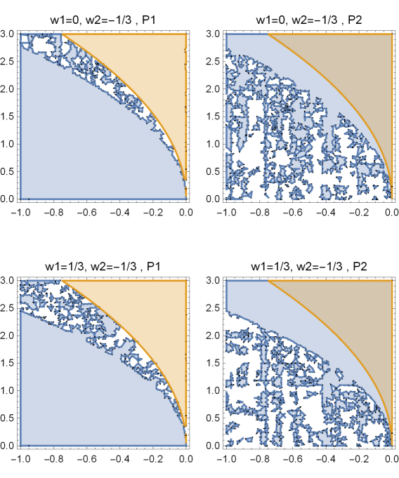
Figure 2: Plot of the region in the space $\left\{\lambda_{0},\lambda_{2}\right\}~{}$where the eigenvalues of the linearized system (19)-(20) are negative. The first line is for $w_{1}=0$ and $w_{2}=\frac{1}{3}$, while the second line is for $w_{1}=\frac{1}{3}$ and $w_{2}=0$. The plots in the left column corresponds to the point $P_{1}$, and the plots in the right column to the point $P_{2}$.  The points are stable only when the colored areas overlap.

Figure 3: Plots of the region in the space $\left\{\lambda_{0},\lambda_{2}\right\}~{}$where the eigenvalues of the linearized system (19)-(20) are negative. The first line is for $w_{1}=0$ and $w_{2}=-\frac{1}{3}$, while the second line is for $w_{1}=\frac{1}{3}$ and $w_{2}=-\frac{1}{3}$. Recall that $w_{2}=-\frac{1}{3}$ corresponds to the scenario of a FLRW universe with non-zero spatial curvature. The plots in the left column corresponds to the point $P_{1}$, and the plots in the right column to the point $P_{2}$. The points are stable only when the colored areas overlap.

Now for $n=1$, Eq. (22)  admits the three critical points

$$P_{1}:\left\{H\left(P_{1}\right)~{},~{}\Omega_{1}\left(P_{1}\right)\right\}=\left\{\frac{1}{3}[(\frac{2\lambda_{0}^{3}}{9\lambda_{2}+\sqrt{81\lambda_{2}^{2}-4\lambda_{0}^{3}}})^{1/3}+(\frac{9\lambda_{2}+\sqrt{81\lambda_{2}^{2}-4\lambda_{0}^{3}}}{2})^{1/3}],0\right\}$$

$$P_{2}:\left\{H\left(P_{2}\right)~{},~{}\Omega_{1}\left(P_{2}\right)\right\}=\left\{\frac{1}{3}[-\frac{(1+\sqrt{-3})\lambda_{0}}{3\sqrt[3]{4}(9\lambda_{2}+\sqrt{81\lambda_{2}^{2}-4\lambda_{0}^{3}})^{1/3}}+(1-\sqrt{-3})(\frac{9\lambda_{2}+\sqrt{81\lambda_{2}^{2}-4\lambda_{0}^{3}}}{432})^{1/3}],0\right\}$$

$$P_{3}:\left\{H\left(P_{3}\right)~{},~{}\Omega_{1}\left(P_{3}\right)\right\}=\left\{\frac{1}{3}[-\frac{(1-\sqrt{-3})\lambda_{0}}{3\sqrt[3]{4}(9\lambda_{2}+\sqrt{81\lambda_{2}^{2}-4\lambda_{0}^{3}})^{1/3}}+(1+\sqrt{-3})(\frac{9\lambda_{2}+\sqrt{81\lambda_{2}^{2}-4\lambda_{0}^{3}}}{432})^{1/3}],0\right\}$$

provided that $\Delta=12\lambda_{0}^{3}-243\lambda_{2}^{2}\geq 0$. Otherwise, when $\Delta<0$, only $P_{1}$ is a real point and describes always a de Sitter Universe.

Furthermore, for $n=2,~{}$the algebraic Eq.(22) admits the four solutions,

$$P_{1\pm}:\left\{H\left(P_{1\pm}\right)~{},~{}\Omega_{1}\left(P_{1\pm}\right)\right\}=\left\{\pm\sqrt{\frac{1}{6}\left(\lambda_{0}-\sqrt{12\lambda_{2}+\lambda_{0}^{2}}\right)},0\right\}$$

$$P_{2\pm}:\left\{H\left(P_{2\pm}\right)~{},~{}\Omega_{1}\left(P_{2\pm}\right)\right\}=\left\{\pm\sqrt{\frac{1}{6}\left(\lambda_{0}+\sqrt{12\lambda_{2}+\lambda_{0}^{2}}\right)},0\right\}.$$

which are de Sitter points for values of $\lambda_{0},~{}\lambda_{2}$ for which the solutions are real. Easily, it follows that when $\lambda_{0},~{}\lambda_{2}$ are positive, then points $P_{2\pm}$ are always real.

When $n=-2$, Eq.(22) provides the critical points $P_{1\pm}:$

$$\left\{H\left(P_{1\pm}\right)~{},~{}\Omega_{1}\left(P_{1\pm}\right)\right\}=\left\{\pm\sqrt{\frac{\lambda_{0}}{3-\lambda_{2}}},0\right\}~{},~{}\text{with }\left\{\lambda_{2}<3,\lambda_{0}>0\right\}\text{ or }\left\{\lambda_{2}>0,\lambda_{0}\right\}.$$

Finally for $n=-3,$ the cubic equation Eq.(22) admits three solutions

$$P_{1}:\left\{H\left(P_{1}\right)~{},~{}\Omega_{1}\left(P_{1}\right)\right\}=\left\{\frac{1}{\lambda_{2}}-\frac{\sqrt[3]{2}}{\lambda_{2}\Sigma\left(\lambda_{0},\lambda_{2}\right)}-\frac{\Sigma\left(\lambda_{0},\lambda_{2}\right)}{\sqrt[3]{2}\lambda_{2}},0\right\},$$

$$P_{2}:\left\{H\left(P_{2}\right)~{},~{}\Omega_{1}\left(P_{2}\right)\right\}=\left\{\frac{1}{\lambda_{2}}+(1+\sqrt{-3})\left(\frac{1}{\sqrt[3]{4}\lambda_{2}\Sigma\left(\lambda_{0},\lambda_{2}\right)}+\frac{\Sigma\left(\lambda_{0},\lambda_{2}\right)}{\sqrt[3]{16}\lambda_{2}}\right),0\right\},$$

$$P_{3}:\left\{H\left(P_{3}\right)~{},~{}\Omega_{1}\left(P_{2}\right)\right\}=\left\{\frac{1}{\lambda_{2}}-\left(1-\sqrt{-3}\right)\left(\frac{{}}{\sqrt[3]{4}\lambda_{2}\Sigma\left(\lambda_{0},\lambda_{2}\right)}-\frac{\Sigma\left(\lambda_{0},\lambda_{2}\right)}{\sqrt[3]{16}\lambda_{2}}\right),0\right\}.$$

where $\Sigma\left(\lambda_{0},\lambda_{2}\right)=(-2+\lambda_{0}\lambda_{2}^{2}+\sqrt{-4\lambda_{0}\lambda_{2}^{2}+\lambda_{0}^{2}\lambda_{2}^{4}})^{1/3}$. Point $P_{1}$ is always real, while $P_{2}$ and $P_{3}$ describe de Sitter Universes when $27\lambda_{0}(4-\lambda_{0}\lambda_{2}^{2})\geq 0.$

IV Singularities and analytical solutions

Technically, in order to study the existence of matter-dominated eras, that is, singular solutions of the form $a\left(\tau\right)=a_{0}\tau^{p},~{}\tau=t-t_{0}$, we apply the ARS algorithm, hence the analytical solution can be written as a Painlevé Series around the (movable) singularity. Moreover, the ARS algorithm provides important information regarding the stability of the singular solution $a\left(\tau\right)=a_{0}\tau^{p}$. The approach of the ARS algorithm is inspired by the work of Kowalevskaya kowa88 , where the solution of a differential equation is described by a power-law function when the differential equation admits a movable singularity. Hence, a necessary condition for the approach to succeed is the existence of at least one movable singularity. The position of the singularity is $t_{0}$, and the singulariy is characterized movable when $t_{0}$ depends on the initial conditions.

The ARS algorithm is developed via a three-step process, a brief description of which is

Step A: The determination of the leading-order behavior. The leading-order term needs to be a negative integer, or at least a non-integral rational number. It is important to point out that the coefficient of the leading-order term may or may not be determined explicitly.

Step B: The proof of the existence of sufficient number of (arbitrary) integration constants by determining the resonances (Fuchs indices). The value minus one should always appear always of one of the resonances. This is important for the singularity to be movable and hence the ARS algorithm to be valid.

Step C: The consistency test is performed by substituting an expansion of the power-law series which describes the solution of the original equation, to test that it is indeed a true solution.

From the leading-order term and the resonances, we can determine the step of the Laurent expansion (Painlevé Series) which describes the actual solution of the original equation. Whereas, the coefficients of the Laurent expansion are determined from the consistency test. For a Right Painlevé Series the resonances must be positive, for a left Painlevé series the resonances must be negative, while for a full Laurent expansion the resonances have to be mixed. Clearly, in the case of an autonomous second-order ordinary equation, since there is only one free resonance, the possible Laurent expansions are either left or right Painlevé series. For more details on the method we refer the reader to the review article of Ramani et al. Ramani 89 .

IV.1 Case A: One ideal fluid

In this case we consider one ideal fluid. In order to determine the movable singularities of Eq.(13) we perform the change of variables, $a\left(t\right)\rightarrow A^{-1}\left(t\right)$, and multiply the equation with the term $A^{2}\left(t\right)\dot{A}^{n}\left(t\right)$ and we find

$$\dot{A}^{n}\left(2A\ddot{A}-\left(5+3w_{1}\right)\dot{A}^{2}+\left(1+w_{1}\right)\lambda_{0}A^{2}\right)-\left(-1\right)^{1-n}\left(1+w_{1}\right)\lambda_{2}A^{2+n}=0.$$ (26)

Then we insert $A\left(\tau\right)=A_{0}\tau^{p}$ in the above equation, where $\tau=t-t_{0}$, and we search for the dominant terms in order to determine the power $p$. Notice, that $t_{0}$ is an integration constant and it denotes the position of the singularity.

IV.1.1 Positive power, $n>0$

For $n>0$ and in the context of $A\left(\tau\right)=A_{0}\tau^{p}$ Eq.(26) then takes the form

$$p^{n+1}\left(3\left(1+w_{1}\right)p+2\right)-p^{n}\tau^{2}\left(1+w_{1}\right)\lambda_{0}-\left(-1\right)^{-n}\left(1+w_{1}\right)\lambda_{2}\tau^{2+n}=0,$$ (27)

from which it follows that the only possible dominant term is that of $p^{n+1}\left[2+3\left(1+w_{1}\right)p\right]$. Therefore if we assume that the leading-order behavior describes explicitly the solution at the singularity then the latter algebraic equation reduces to

$$2+3\left(1+w_{1}\right)p\simeq 0,$$ (28)

or

$$p\simeq-\frac{2}{3\left(1+w_{1}\right)}.$$ (29)

Hence, the singular solution of the ideal fluid, without the $\Lambda$-varying term, describes the actual solution of the model close to the singularity.

For the second step of the ARS algorithm, we substitute $A\left(\tau\right)=A_{0}\tau^{-\frac{2}{3\left(1+w_{1}\right)}}+m\tau^{-\frac{2}{3\left(1+w_{1}\right)}+s}$, and we linearize around $m=0$. From the remaining terms, we find that the coefficient of the leading-order term vanishes if and only if

$$s\left(s+1\right)=0$$ (30)

which means that the resonances are $s_{1}=-1$ and $s_{2}=0$. The second resonance tells us that the second integration constant is the coefficient $A_{0}$, of leading-order term. We show that equation (28) is not affected by $A_{0}$, hence this constant is arbitrary. In this case the analytical solution of Eq.(26) is given by a right Laurent expansion, while its step depends on $w_{1}$. Notice, that the presence of a right Painlevé series means that the matter-dominated era close to the singularity, is an unstable solution. We note that the problem contains two integration constants, namely $A_{0}$ and $w_{1}$, hence it is not necessary to perform the consistency test. Below, we complete the current analysis by presenting some analytical solutions which are physically interesting.

Analytic solution for a non-relativistic fluid:

For a pressureless matter source, we have $w_{1}=0$. Therefore, from Eq.(29) we calculate $p=-\frac{2}{3}$, which means that the Laurent expansion has a step of $\frac{1}{3}$, that is, the solution of (26) is

$$A\left(\tau\right)=A_{0}\tau^{-\frac{2}{3}}+A_{1}\tau^{-\frac{1}{3}}+A_{2}+A_{3}\tau^{\frac{1}{3}}+{\displaystyle\sum\limits_{I=4}^{\infty}}A_{k}\tau^{-\frac{2}{3}+\frac{\nu}{3}},$$ (31)

where we need to determine the coefficients $A_{1},A_{2},..$ etc.

In the case of the $\Lambda-$varying model (11), with $n=1$, the first six non-zero coefficients of (31) are: $A_{0}$, which is an arbitrary integration constant, and

$$\frac{A_{6}}{A_{0}}=-\frac{\lambda_{0}}{12},~{}\frac{A_{9}}{A_{0}}=-\frac{\lambda_{2}}{16},~{}\frac{A_{12}}{A_{0}}=\frac{\left(\lambda_{0}\right)^{2}}{180},$$

$$\frac{A_{15}}{A_{0}}=\frac{7\lambda_{0}\lambda_{2}}{480}~{}\text{and~{}}\frac{A_{18}}{A_{0}}=\frac{23895\lambda_{2}^{2}-1072\lambda_{0}^{3}}{2903040}A_{0},~{}etc.,$$

while the rest of non-zero coefficients are those of $A_{21+3\nu}$, $\nu\in\mathbb{N}.$On the other hand, for other values of the power $n$, the coefficients are different. For example, in the case of the $\Lambda(H)$ model with $n=3$, aside from $A_{0},$ the first non-zero coefficients are

$$\frac{A_{6}}{A_{0}}=-\frac{\lambda_{0}}{12},~{}\frac{A_{12}}{A_{0}}=\frac{\lambda_{0}^{2}}{180},~{}\frac{A_{15}}{A_{0}}=-\frac{9\lambda_{2}}{160}~{}$$

$$\frac{A_{18}}{A_{0}}=-\frac{67\lambda_{0}^{2}}{181440},~{}etc.,$$

while the other non-zero coefficients are $A_{18+3\nu}$, $\nu\in\mathbb{N}.$

From the aforementioned solutions, we observe that the solution close to the matter-dominated era includes an additional term $A_{0}\tau^{\frac{4}{3}}$, namely

$$A\left(\tau\right)\simeq A_{0}\tau^{-\frac{2}{3}}+A_{6}\tau^{\frac{4}{3}}$$ (32)

and so the scale factor is written as a Taylor expansion around $\tau=0$ as follows,

$$a\left(\tau\right)\simeq a_{0}\tau^{\frac{2}{3}}+a_{6}\tau^{\frac{8}{3}}.$$ (33)

Analytic solution for a radiation fluid:

Considering that the ideal fluid is radiation ($w_{1}=1/3$) from (29), we obtain $p=-\frac{1}{2}$, which means that the solution is expressed by a right Painlevé series with step $\frac{1}{2}$, that is,

$$A\left(\tau\right)=\bar{A}_{0}\tau^{-\frac{1}{2}}+\bar{A}_{1}+\bar{A}_{2}\tau^{\frac{1}{2}}+\bar{A}_{3}\tau+{\displaystyle\sum\limits_{I=4}^{\infty}}\bar{A}_{I}\tau^{-\frac{1}{2}+\frac{\nu}{2}},$$ (34)

where $\bar{A}_{0}$ is an integration constant.

For $n=1$, the nonzero coefficients of the expansion (34) are

$$\frac{\bar{A}_{4}}{\bar{A}_{0}}=-\frac{\lambda_{0}}{9}~{},~{}\frac{\bar{A}_{6}}{\bar{A}_{0}}=-\frac{\lambda_{2}}{9}~{}\ ,~{}\frac{\bar{A}_{8}}{\bar{A}_{0}}=\frac{\lambda_{0}^{2}}{90}~{},~{}\frac{~{}\bar{A}_{10}}{\bar{A}_{0}}=\frac{17\lambda_{0}\lambda_{2}}{405},$$

$$\frac{\bar{A}_{12}}{\bar{A}_{0}}=\frac{1665\lambda_{2}^{2}-61\lambda_{0}^{3}}{51030},~{}~{}\frac{\bar{A}_{14}}{\bar{A}_{0}}=-\frac{221\lambda_{0}^{2}\lambda_{2}}{17010}.\mathbb{N}.$$

For $n=2$, the coefficients of the expansion are

$$\frac{\bar{A}_{4}}{\bar{A}_{0}}=-\frac{\lambda_{0}}{9}~{},~{}\frac{\bar{A}_{8}}{\bar{A}_{0}}=\frac{\lambda_{0}^{2}-12\lambda_{2}}{90}~{},~{}\frac{\bar{A}_{12}}{\bar{A}_{0}}=\frac{4212\lambda_{0}\lambda_{2}-61\left(\lambda_{0}\right)^{3}}{51030},$$

$$\frac{\bar{A}_{16}}{\bar{A}_{0}}=\frac{1261\lambda_{0}^{4}-362664\lambda_{0}^{4}\lambda_{2}+879984\lambda_{2}^{2}}{9185400}\mathbb{N}.$$

Therefore, the analytical solution prior to the radiation era is well approximated by the following expression:

$$A\left(\tau\right)=\bar{A}_{0}\tau^{-\frac{1}{2}}\left(1-\frac{\lambda_{0}}{9}\tau^{2}\right),$$

and so

$$a\left(\tau\right)\simeq a_{0}\tau^{\frac{1}{2}}+a_{1}\tau^{\frac{5}{2}}.$$ (35)

IV.1.2 Negative power, $n<0$

Now we study the case where the exponent $n$ in $\Lambda(H)=\lambda_{0}+\lambda_{2}H^{-n}$ is negative. We remind the reader that we are still using the variable $A\left(\tau\right)=A_{0}\tau^{p}$. Under those conditions Eq.(26) gives

$$\tau^{\left(2-n\right)\left(p-1\right)}\left[\left(3\left(1+w_{1}\right)p+2\right)p\tau^{-n}-\left(1+w_{1}\right)\lambda_{0}\tau^{2-n}-\left(-1\right)^{-n}\tau p^{-n}\left(1+w_{1}\right)\lambda_{2}\tau^{2}\right]=0.$$ (36)

Following similar notations to those of section 4.1.1 we find that the only possible leading term is the one with coefficient $2+3\left(1+w_{1}\right)p$ as long as $n>-2$, which implies that the exponent $p$ is given by Eq.(29). As expected, from the ARS algorithm, we find that the constant $A_{0}$ is arbitrary, hence the corresponding resonances (30) are $s_{1}=-1$ and $s_{2}=0$ respectively, whilst the analytical solution is written as a right Painlevé series. Specifically, we find the following interesting solutions.

Analytic solution for a non-relativistic fluid:

For $w_{1}=0,$ the Laurent expansion is of the form of (31), where with $n=-1$, namely $\Lambda(H)=\lambda_{0}+\lambda_{2}H$, we obtain the following coefficients:

$$\frac{A_{3}}{A_{0}}=-\frac{\lambda_{2}}{6}~{},~{}\frac{A_{6}}{A_{0}}=\frac{\lambda_{2}^{2}-12\lambda_{0}}{144}~{},~{}\frac{A_{9}}{A_{0}}=\frac{\lambda_{2}^{3}+36\lambda_{0}\lambda_{2}}{2592}~{},$$

$$\frac{A_{12}}{A_{0}}=\frac{216\lambda_{0}^{2}-9\lambda_{0}\lambda_{2}^{2}-\lambda_{2}^{3}}{38880}~{}.\mathbb{N}$$

This means that close to the singularity the scale factor is approximated by

$$a\left(\tau\right)\simeq a_{0}\tau^{\frac{2}{3}}+a_{3}\tau^{\frac{5}{3}}.$$ (37)

Notice that the second term of this solution is different with that of Eq.(33) for $n>0$. The closed-form solution in the case of the $\Lambda(H)=\lambda_{0}+\lambda_{2}H$ running-vacuum model has been found earlier in gomez . In this case the running vacuum model introduces a mild dynamical behavior of the vacuum energy at low energies, namely dark matter and dark energy eras. For more details regarding the dynamics as well as the corresponding observational constraints of the current vacuum model we refer the reader the work of gomez . On the other hand, terms of the form $H^{3}$, $H^{4}$ ($n<-2$) they can be important for the early universe (see perico and Sahni2014 ).

Analytic solution for a radiation fluid:

Here, the equation of state parameter (hereafter EoS) is $w_{1}=\frac{1}{3}$, and the analytical solution is given by the series (34). For $n=-1,$ the corresponding non-zero coefficients are

$$\frac{\bar{A}_{2}}{A_{0}}=-\frac{\lambda_{2}}{6},~{}\frac{\bar{A}_{4+2\nu}}{A_{0}}\neq 0~{}\nu\in\mathbb{N},$$

and so, prior to the radiation-dominated era (singular solution), the scale factor can be written as

$$a\left(\tau\right)\simeq a_{0}\tau^{\frac{1}{2}}+a_{2}\tau^{\frac{3}{2}}.$$ (38)

Again, this solution includes an extra term which differs from Eq.(35) for $n>0$.

At this point the following comments are appropriate. The current approximate solutions (37)-(38), for non-relativistic matter and radiation contain extra terms which differ from those in (33) and (35) where $n=1$. This is expected: for negative powers of $n$, the extra terms of the solutions are related to the $\lambda_{2}H^{-n}$ term in Eq.(11), while for $n>0$ the extra terms are affected by the constant vacuum term $\lambda_{0}$. However, in this case the $\lambda_{0}$ term is introduced in the second-order correction to the solution, which means that there are differences between the two solutions $\lambda_{0}=0$ and $\lambda_{0}\neq 0$, not very far from the singularity. In order to understand the differences between the two solutions, in Fig. 4 we present the evolution of the relative difference between the numerical simulations for $n=-1$, and $\lambda_{0}=0$ and those with $\lambda_{0}\neq 0$, for the scale factor and the Hubble expansion rate.

We observe that prior to the singularity the relative error is close to the error of the numerical integration; however, as the system evolves the relative error becomes larger. In the left panel of Fig. 5 we plot the evolution of the scale factors which are considered in Fig. 4, while in the right panel of Fig. 5 we show the relative difference in the energy density $\Omega_{\Lambda}=\Lambda\left(H\right)/3H^{2}$ between the different solutions.

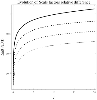
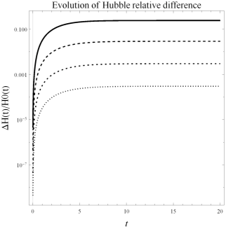
Figure 4: Qualitative evolution in time for the relative difference between the solutions of the master equation (12) for $\lambda_{0}=0$, with $\lambda_{0}\neq 0$ and $n=-1$. Left Fig. is for the scale factors while Right Fig. for the Hubble functions. For the numerical integration we considered $\lambda_{2}=1$, while the solid line provides the relative error of solution with $\lambda_{0}=10^{-1}\lambda_{2},~{}$dash-dash line for $\lambda_{0}=10^{-2}\lambda_{l}$, dot-dot line for $\lambda_{0}=10^{-3}\lambda_{2}$ and the dash-dot line for $\lambda_{0}=10^{-4}\lambda_{2}$. For the numerical integration we started close to the singular solution with $w_{1}=\frac{1}{3}$, that is, at the radiation epoch.

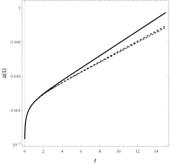
Figure 5: Qualitative evolution in time for the scale factor $a(t)$ (Left Fig.) and the relative difference of the energy density $\Omega_{\Lambda}\left(t\right)$ for the solutions which were presented in Fig. (4). For the numerical integration we have considered $\lambda_{2}=1$, $n=-1$, while the solid line provides the relative error of the solution with $\lambda_{0}=10^{-1}\lambda_{2},~{}$the dash-dash line for $\lambda_{0}=10^{-2}\lambda_{2}$, the dot-dot line for $\lambda_{0}=10^{-3}\lambda_{2}$ and the dash-dot line for $\lambda_{0}=10^{-4}\lambda_{2}$. We started the numerical integration close to the singular solution with $w_{1}=\frac{1}{3}$, that is, at the radiation epoch.

Recall that $\lambda_{0}$ does not correspond to the value of the cosmological constant at the present time. In particular, the latter is given by $\Lambda\left(H_{0}\right)=\lambda_{0}+\lambda_{2}H_{0}^{-n}$, where $H_{0}$ is the value of the Hubble function at the present time. Therefore, since we know that $\Lambda\left(H_{0}\right)$ is small, we must have $\lambda_{0}$ of the order of $\lambda_{2}H_{0}^{-n}$: that is, for $n<0$, $\left|\lambda_{0}\right|>\left|\lambda_{2}\right|.$ This makes clear that the correction terms which depend on $\lambda_{0}$ are important for the evolution of the system.

The singularity analysis fails for $n<-2$, and below we will carry out our analysis for the case of two ideal fluids.

IV.2 Case B: Two ideal gases

In this section we consider that the cosmic fluid consists two ideal fluids, where one of them is minimally coupled (see Case B in section 2). In this case using the transformation $A\left(t\right)=a^{-1}\left(t\right)$, the second-order differential equation (18) becomes

$$\dot{A}^{n}[2A\ddot{A}-\left(5+3w_{1}\right)\dot{A}^{2}+\left(1+w_{1}\right)\lambda_{0}A^{2}+w_{2}\rho_{20}A^{3\left(1+w_{2}\right)}]-\left(-1\right)^{-n}\left(1+w_{1}\right)\lambda_{2}A^{2-2n}=0.$$ (39)

Using $\tau=t-t_{0}$ and substituting $A\left(t\right)=A_{0}\tau^{p}$ in (39), we find the expression

$$\tau^{-3+\left(3+n\right)p}\left[p^{n+1}\left(3\left(1+w_{1}\right)p-2\right)-p^{n}\tau^{2}\left(\left(1+w_{1}\right)\lambda_{2}-w_{2}\rho_{20}A_{0}^{3\left(1+w_{2}\right)}\tau^{3\left(1+w_{2}\right)p}\right)-\left(-1\right)^{n}\left(1+w_{1}\right)\lambda_{2}\tau^{2+n}\right]=0.$$ (40)

This provides the following three dominant behaviors:

IV.2.1 Positive power, $n>0,$ solution I

For $n>0$, if we assume that the dominant term close to the singularity is $2+3(1+w_{1})p$, then $p$ is given by Eq.(29). This implies that the singular solution describes the matter-dominated era via the fluid $\rho_{1}\left(t\right)$. Of course we need to clarify that the above term is indeed the dominant one if and only if the corresponding EoS parameters of the two ideal fluids satisfy the inequality

$$w_{2}<w_{1}.$$ (41)

Within the framework of this latter restriction we present some special analytical solutions, below. It is important to mention that when $w_{2}=-\frac{1}{3}$, Eq.(18) corresponds to that of one ideal effective fluid in a FLRW spacetime with nonzero spatial curvature $k$, such that $k=-\rho_{20}$.

For the calculation of the resonances, we follow standard steps; namely, we substitute $A\left(t\right)=A_{0}\tau^{-\frac{2}{3\left(1+w_{1}\right)}}\left(1+mt^{s}\right)$ in (39) and from the coefficient of the dominant term in the linearized equation around the value $m=0$ we obtain $s\left(1+s\right)=0$, hence the two resonances are $-1$ and $0$.

Because the second resonance has the value zero, the second integration constant is the coefficient of the dominant term; hence, it is not necessary to perform the consistency test. However, in order to compare the current solutions with those of Case A we shall now investigate some applications.

Analytic solution for a non-relativistic fluid and curvature term:

Here, we have $(w_{1},w_{2})=(0,-\frac{1}{3})$. Therefore, the leading-order term is $p=-\frac{2}{3}$ and the step of the expansion is $\frac{1}{3}$. The analytical solution is given by expression (31) while, for $n=1,$ the nonzero coefficients of the Laurent expansion are given by

$$\frac{A_{2}}{A_{0}}=-\frac{3A_{0}^{2}\rho_{20}}{20}~{},~{}\frac{A_{4}}{A_{0}}=\frac{9\left(A_{0}^{2}\rho_{20}\right)^{2}}{280}~{},~{}\frac{A_{6}}{A_{0}}=-\frac{100\lambda_{0}+9\left(A_{0}^{2}\rho_{20}\right)^{3}}{1200},$$

$$\frac{A_{8}}{A_{0}}=\frac{9\left(39200\lambda_{0}+3483\left(A_{0}^{2}\rho_{20}\right)^{3}\right)\left(A_{0}^{2}\rho_{20}\right)}{17248000}\mathbb{N}.$$

Notice that the other non-zero coefficients of the series have the form $A_{10+2\nu}$, $\nu\in\mathbb{N}.$ Recall that the constraint (3) provides an algebraic relation between the free parameters of the model. As expected, for $k=\rho_{20}=0$ the current solution reduces to that of section 3.1, while close to the singularity, and for $k=\rho_{20}\neq 0,$ the approximated solution is

$$A\left(\tau\right)=A_{0}\tau^{-\frac{2}{3}}+A_{2},$$ (42)

or

$$a\left(\tau\right)=a_{1}\tau^{\frac{2}{3}}+a_{2}\tau^{\frac{4}{3}}.$$ (43)

Analytic solution for radiation and non-relativistic matter:

Now, we assume that $\rho_{1}\left(t\right)$ and $\rho_{2}\left(t\right)$ are the radiation ($w_{1}=\frac{1}{3}$) and matter ($w_{2}=0$) densities respectively. In this case, the solution of the problem are the series (34) with $\bar{A}_{0}$ arbitrary and for $n=1$ the nonzero coefficients are found to be

$$\frac{\bar{A}_{4}}{\bar{A}_{0}}=-\frac{\lambda_{0}}{9}~{},~{}\frac{\bar{A}_{6}}{\bar{A}_{0}}=-\frac{\lambda_{2}}{9}~{},~{}\frac{\bar{A}_{8}}{\bar{A}_{0}}=\frac{\lambda_{0}^{2}}{90}\mathbb{N},$$

while the other non-zero coefficients take the form $A_{10+2\nu}$, $\nu\in\mathbb{N}.$

Analytic solution for radiation and curvature term:

Here we consider that the cosmic fluid contains radiation ($w_{1}=\frac{1}{3}$) and curvature ($w_{2}=-\frac{1}{3}$). Again, if in the case of the dust we consider another fluid, for instance $w_{2}=-\frac{1}{3}$, which corresponds to the curvature term, then the analytical solution is given by Eq.(34) with the following nonzero coefficients (for $n=1$),

$$\frac{\bar{A}_{2}}{\bar{A}_{0}}=-\frac{A_{0}^{2}\rho_{20}}{12}~{},~{}\frac{\bar{A}_{4}}{\bar{A}_{0}}=-\frac{32\lambda_{0}-3\left(A_{0}^{2}\rho_{20}\right)^{2}}{288}~{},$$

$$\frac{\bar{A}_{6}}{\bar{A}_{0}}=\frac{64\lambda_{0}A_{0}^{2}\rho_{20}-5\left(A_{0}^{2}\rho_{20}\right)^{3}-384\lambda_{2}}{3456}\mathbb{N},$$

where we clearly observe the differences with respect to that of the previous solution (radiation and non-relativistic matter).

IV.2.2 Positive power, $n>0,$ solution II

The second class of solutions are those for which the leading-order terms of Eq. (40) are $-3+\left(3+n\right)p$ and $-1+p\left[3\left(2+w_{2}\right)+n\right]$. Keeping only these terms, Eq. (40) reduces to

$$-3+\left(3+n\right)p\simeq-1+p\left[3\left(2+w_{2}\right)+n\right],$$ (44)

and so

$$p\simeq-\frac{2}{3\left(1+w_{2}\right)}.$$ (45)

Therefore, that new singular solution describes the matter-dominated era of the minimally coupled fluid $\rho_{2}\left(t\right)$.

In contrast to the aforementioned cases, the constant $A_{0}$ here is not arbitrary but it is given in terms of $w_{1}$, $w_{2}$ and $\rho_{20}$, by

$$\rho_{20}=\frac{4A_{0}^{-3\left(1+w_{2}\right)}\left(w_{2}-w_{1}\right)}{3w_{2}\left(1+w_{2}\right)^{2}},$$ (46)

where $w_{2}\neq 0$. Since $A_{0}$ is not arbitrary, we expect that the second resonance cannot be zero. Indeed, using our methodology we find the following resonances:

$$s_{1}=-1~{}~{},~{}~{}s_{2}=2\frac{\left(w_{2}-w_{1}\right)}{1+w_{2}}.$$ (47)

Unlike the previous cases, where the corresponding solutions are written as right Painlevé series, we have a different situation here. In particular, if we select the EoS parameters $(w_{1},w_{2}$) such that $s_{2}<0,$ then the solution is given by a left Painlevé series and thus the dominant term is an attractor.

Analytic solution for radiation and curvature:

Using $w_{1}=\frac{1}{3}$ and $w_{2}=-\frac{1}{3}$ Eqs.(45) and (47) provide $p=-1$ and $s_{1}=-1$, $s_{2}=1$. Therefore, the analytical solution is

$$A\left(\tau\right)=A_{0}\tau^{-1}+A_{1}+A_{2}\tau+A_{3}\tau^{2}+{\displaystyle\sum\limits_{v=4}^{\infty}}A_{v}\tau^{-1+\nu}.$$ (48)

Notice, that the solution passes the consistency test. Moreover, the fact that the second resonance is positive implies that the solution (48) is unstable. Now, using the dominant term $A\simeq A_{0}\tau^{-1}$ of the above solution, i.e. $a(\tau)\propto\tau,~{}$we find that the Milne universe and the $R_{h}=ct$ model Melia can be seen as perturbations around the present $\Lambda(H)$ model.

If the $R_{h}=ct$ or Milne models were somehow the effective behavior of the current $\Lambda(H)$ model, then we could argue that the $R_{h}=ct$ and Milne models are both unstable.

To this end, for $n=1$ the nonzero coefficients of (48) are, $A_{1}$ which is the second integration constant and

$$A_{2}=\frac{27A_{1}^{2}-2A_{0}^{2}\lambda_{0}}{18A_{0}}~{},~{}A_{3}=\frac{90A_{1}^{3}-8A_{0}^{2}A_{1}\lambda_{0}-3A_{0}^{3}\lambda_{2}}{36A_{0}^{2}}~{},~{}etc,$$

where $A_{1}$ is a second integration constant.

IV.2.3 Negative power, $n<0$

The last case that we have to consider is when the power $n$ is negative, i.e. $n<0$. In this case it follows that the only possible dominant behavior is that with $p=-\frac{2}{3\left(1+w_{1}\right)}$, while the corresponding resonances are $s_{1}=-1$ and $s_{2}=0$, which means that the second integration constant is the $A_{0}$ coefficient. Thus, since we know the two integration constants explicitly it is not necessary to perform step C of the ARS algorithm, i.e. the consistency test. However, for the completeness of our analysis we present the Laurent expansions for two cases of special interest.

Analytic solution for radiation and nonrelativistic matter

If we assume that $\ w_{1}=\frac{1}{3}$ and $w_{2}=0$, then the dominant behavior is $p=-\frac{1}{2}$, and the solution is given as a right Painlevé series with step $\frac{1}{2}$, that is, series (34), where now the first nonzero coefficients for $n=-1$ are

$$\frac{\bar{A}_{2}}{A_{0}}=-\frac{\lambda_{2}}{6}~{},~{}\frac{\bar{A}_{4}}{A_{0}}=\frac{\lambda_{2}^{2}-24\lambda_{0}}{216}~{},~{}A_{6}=\frac{\lambda_{2}^{3}+24\lambda_{0}\lambda_{2}}{1296},~{}etc.$$

Analytic solution for radiation and curvature

In a similar way, for $w_{1}=\frac{1}{3}$ and $w_{2}=-\frac{1}{3}$, the solution is given by the right Painlevé series (34) with step $\frac{1}{2}$, where the first nonzero coefficients for $n=-1$ are

$$\frac{\bar{A}_{2}}{A_{0}}=-\frac{2\lambda_{2}+A_{0}^{2}\rho_{20}}{12}~{},~{}\frac{\bar{A}_{4}}{A_{0}}=\frac{4\lambda_{2}^{2}-96\lambda_{0}+20A_{0}^{2}\rho_{20}+9A_{0}^{4}\rho_{20}^{2}}{864},~{}etc.$$

In the following section we discuss our results and we draw our conclusions.

V Conclusions

In the framework of running vacuum ($\Lambda$) models we implemented a critical point analysis in order to study the existence and the stability of singular solutions which describe de Sitter, radiation and matter dominated eras. We used one of the most popular expressions for the vacuum parameter which describes a large family of running vacuum models, namely $\Lambda(H)=c_{0}+c_{1}H^{2}+c_{2}H^{-n}$. We showed that this functional form of $\Lambda(H)$ allows for a number of de Sitter eras, depending on the model parameters. The radiation and matter dominated eras are also investigated with the method of singularity analysis. In order to recover a sequence of radiation and matter eras, we found some interesting constraints on the cosmic fluid.

Furthermore, it is interesting to mention that a closed form solution exists only under special conditions. Indeed, analytical solutions (see perico and gomez ) are possible when the cosmic fluid contains only two components, namely one fluid (non-relativistic or radiation) and running vacuum $\Lambda(H)$. Also, in the case of perico we have an additional restriction towards solving analytically the Friedamnn equations, namely we are dealing only with even powers in $H$, hence the term $\lambda_{2}H^{-n}$ boils down to $\lambda_{2}H^{2k}$ with $n=-2k$ and $k\geq 2$ [see Eq.(7)]. Despite the fact that the above special solutions are available, we are unaware of any study concerning the critical points in running vacuum cosmologies. Moreover, if the cosmic fluid includes radiation, non-relativistic matter and running vacuum $\Lambda(H)$ (this situation is close to reality) then analytical solutions are not yet available, implying that the approximated solutions of the present study are completely new and novel.

In this context, we found families of $\Lambda(H)$ cosmologies for which new analytical solutions are given in terms of Laurent expansions. Finally, we showed that the Milne universe and the $R_{h}=ct$ model can be written as perturbations deviating from a special, but unstable, $\Lambda(H)$ model.

References

• (1) S. Perlmutter, et al., Astrophys. J. 517, 565 (1998)
• (2) A. G. Riess, et al., Astron J. 116, 1009 (1998)
• (3) P. Astier et al., Astrophys. J. 659, 98 (2007)
• (4) N. Suzuki et al., Astrophys. J. 746, 85 (2012)
• (5) E. Komatsu et al., Astrophys. J. Suppl. 192, 18 (2011)
• (6) P.A.R. Ade et al. A&A. 571, A16 (2014)
• (7) G.W. Horndeski, Int. J. Theor. Phys. 10, 363 (1974)
• (8) C. Brans and R.H. Dicke, Phys. Rev. 124, 195 (1961)
• (9) A. Nicolis, R. Rattazzi and E. Trincherini, Phys. Rev. D 79, 064036 (2009)
• (10) L. Arturo Urena-Lopez, J. Phys. Conf Ser. 761, 012076 (2016)
• (11) T. Clifton, P.G. Ferreira, A. Padilla and C. Skordis, Phys. Rep. 513, 1 (2012)
• (12) T.P. Sotiriou and V. Faraoni, Rev. Mod. Phys. 82, 451 (2010)
• (13) G.R. Bengochea and R. Ferraro, Phys. Rev. D 79, 124019 (2009)
• (14) H.A. Buchdahl, Mon. Not. Roy. astron. Soc. 150, 1 (1970)
• (15) R.C. Nunes, A. Bonilla, S. Pan and E.N. Saridakis, EPJC 77, 230 (2016)
• (16) R.C. Nunes, S. Pan and E.N. Saridakis, JCAP 1608, 011 (2016)
• (17) P. J. Peebles and B. Ratra, Rev. Mod. Phys. 75, 559, (2003)
• (18) S. Weinberg, Rev. Mod. Phys. 61, 1 (1989)
• (19) T. Padmanabhan, Phys. Rept. 380, 235 (2003)
• (20) L. Perivolaropoulos, arXiv:0811.4684
• (21) A. Padilla, arXiv:1502.05296
• (22) M. Ahmed, S. Dodelson, P.B. Greene and R. Sorkin, Phys. Rev. D 69, 103523 (2004)
• (23) J. Solà, J.Phys. A 41 (2008) 164066
• (24) J. Sola, J. Phys. Conf. Ser. 283, 012033 (2011)
• (25) I. L. Shapiro and J. Sola, Phys. Lett. B 530, 10 (2002)
• (26) A.A. Starobinsky, Phys. Lett. B91, 99 (1980)
• (27) S. Basilakos, M. Plionis and J. Sola, Phys. Rev D. 80, 083511 (2009)
• (28) S. Basilakos, Astron. & Astrophys., 508, 575 (2009)
• (29) E.L.D. Perico, J.A.S. Lima, S. Basilakos and J. Sola, Phys. Rev. D 88, 063531 (2013)
• (30) M. Ozer and O. Taha, Phys. Lett. A 171, 363 (1986) Nucl. Phys. B 287, 776 (1987)
• (31) O. Bertolami, Nuovo Cimento 93, 36 (1986)
• (32) W. Chen and Y.S. Wu, Phys. Rev. D 41, 695 (1990)
• (33) J. A. S. Lima and J. C. Carvalho, Gen. Rel. Grav. 26,909 (1994)
• (34) J. A. S. Lima, J. M. F. Maia and N. Pires, IAU Symposium 198, 111 (2000)
• (35) J. V. Cunha, J.A. S. Lima and N. Pires, Astron. and Astrophys. 390,809 (2002)
• (36) M. V. John and K. B. Joseph, Phys. Rev. D 61, 087304 (2000)
• (37) M. Novello, J. Barcelos-Neto and J. M. Salim, Class. Quant. Grav. 18, 1261 (2001)
• (38) R. G. Vishwakarma, Class. Quant. Grav. 18, 1159 (2001)
• (39) R. Aldrovandi, J. P. Beltran Almeida and J.G. Pereira, Grav. Cosmol. 11, 277 (2005)
• (40) R. Schutzhold, Phys. Rev. Lett. 89, 081302 (2002)
• (41) R. Schutzhold, Int. J. Mod. Phys. A 17, 4359 (2002)
• (42) J. C. Carvalho, J. A. S. Lima, and I. Waga, Phys. Rev. D 46, 2404 (1992)
• (43) J. A. S. Lima and J. M. F. Maia, Mod. Phys. Lett. A 08, 591 (1993)
• (44) J. A. S. Lima and M. Trodden, Phys. Rev. D 53, 4280 (1996)
• (45) S. Carneiro, J.A.S. Lima,  Int. J. Mod. Phys. A 20, 2465 (2005)
• (46) J. Salim and I. Waga, Class. Quant. Grav. 10, 1767 (1993)
• (47) R. C. Arcuri and I. Waga, Phys. Rev. D 50, 2928 (1994)
• (48) S. Pan, MPLA 33, 1850003 (2018)
• (49) M.J. Ablowitz, A. Ramani and H. Segur,  Lett. al Nuovo Cimento 23, 333 (1978)
• (50) M.J. Ablowitz, A. Ramani and H. Segur, J. Math. Phys. 21, 715 (1980)
• (51) M.J. Ablowitz, A. Ramani and H. Segur, J. Math. Phys. 21, 1006 (1980)
• (52) S. Cotsakis and P.G.L. Leach, J. Phys. A 27, 1625 (1994)
• (53) S. Cotsakis, J. Demaret, Y. De Rop and L. Querella, Phys. Rev. D 48, 4595 (1993)
• (54) J.D. Barrow, S. Cotsakis and A. Tsokaros, Class. Quantum Grav. 27, 165017 (2010)
• (55) A. Paliathanasis, J.D. Barrow and P.G.L. Leach, Phys. Rev. D 94, 023525 (2016)
• (56) A. Paliathanasis, EPJC 77, 438 (2017)
• (57) A. Paliathanasis, S. Pan and J.D. Barrow, Phys. Rev. D 95, 103516 (2017)
• (58) J.A.S. Lima, S. Basilakos and J. Sola, Mon. Not. Roy. Astr. Soc. 431, 923 (2013)
• (59) S. Kowalevski, Acta. Math. 12, 177 (1889)
• (60) A. Ramani, B. Grammaticos and T. Bountis, Phys. Rep. 180, 159 (1989)
• (61) T.C. Bountis and L.B. Drossos, J. Nonlin. Sci., 7, 45 (1997)
• (62) K. Andriopoulos and P.G.L. Leach, Phys. Lett. A, 359, 199 (2006)
• (63) K. Andriopoulos and P.G.L. Leach, J. Phys. A: Math. Theor. 41, 155201 (2008)
• (64) M. Gasperini, Phys. Lett. B 194 (1987) 347
• (65) A. Paliathanasis and P.G.L. Leach, Phys. Lett. A 381, 1277 (2017)
• (66) A. Gomez-Valent, J. Sola and S. Basilakos, JCAP 01, 004 (2015)
• (67) S. Basilakos, J. Lima and J. Sola, Int.J.Mod.Phys. D22 (2013) 1342008; S. Basilakos, N. Mavromatos and J. Sola, Universe, 2 14 (2016)
• (68) A. Gomez-Valent and J. Sola, Mon. Not. Roy astron. Soc. 448, 2810 (2015)
• (69) J. Sola, A. Gomez-Valent and J. de Cruz Pérez, Astrophys.J. 836 (2017) 43
• (70) Gong-Bo Zhao et al., Nat. Astron. 1, 627 (2017)
• (71) J. Sola, Cosmological constant and vacuum energy: old and new ideas , J. Phys. Conf. Ser. 453, 012015 (2013) [e-Print: arXiv:1306.1527]; Vacuum energy and cosmological evolution , AIP Conf.Proc. 1606 (2014) 19 [e-Print: arXiv:1402.7049]; J. Grande J. Sola, S. Basilakos and M. Plionis, JCAP, 08, 007 (2011)
• (72) S. Carneiro, M. A. Dantas, C. Pigozzo and J. S. Alcaniz, Phys. Rev. D., 77, 083504, (2008); H. A. Borges, S. Carneiro, J. C. Fabris, Phys. Rev. D 78, 123522, (2008)
• (73) S. Basilakos, Mon. Not. Roy. astron. Soc. 395, 2347, (2009)
• (74) F. Melia, Mon. Not. Roy. astron. Soc. 446, 1191 (2015)
• (75) V. Sahni, A. Shafieloo and A. A. Starobinsky, Astrophys. J. 793, L40 (2014)