Estimation of the Number of Communities
in the Stochastic Block Model

Abstract

In this paper we introduce an estimator for the number of communities in the Stochastic Block Model (SBM), based on the maximization of a penalized version of the so-called Krichevsky-Trofimov mixture distribution. We prove its eventual almost sure convergence to the underlying number of communities, without assuming a known upper bound on that quantity. Our results apply to both the dense and the sparse regimes. To our knowledge this is the first consistency result for the estimation of the number of communities in the SBM in the unbounded case, that is when the number of communities is allowed to grow with the same size.

I Introduction

In this paper we address the model selection problem for the Stochastic Block Model (SBM); that is, the estimation of the number of communities given a sample of the adjacency matrix. The SBM was introduced by [1] and has rapidly popularized in the literature as a model for random networks exhibiting blocks or communities between their nodes. In this model, each node in the network has associated a latent discrete random variable describing its community label, and given two nodes, the possibility of a connection between them depends only on the values of the nodes’ latent variables.

From a statistical point of view, some methods have been proposed to address the problem of parameter estimation or label recovering for the SBM. Some examples include maximum likelihood estimation [2, 3], variational methods [4, 5], spectral clustering [6] and Bayesian inference [7]. The asymptotic properties of these estimators have also been considered in subsequent works such as [8] or [9]. In [10] the reader can find an overview of recent approaches and theoretical results concerning the problem of community detection in SBMs. All these approaches assume the number of communities is known a priori.

The model selection problem, that is the estimation of the number of communities, has been also addressed before using different approaches. Some examples include methods based on the spectrum of the graph [11, 12, 13] or cross validation [14, 15]. From a Bayesian perspective, in [4] the authors propose a criterion known as Integrated Completed Likelihood (ICL) based on the previous work [16] for clustering, where a penalized profile likelihood function is used as approximation of the ICL. To our knowledge it was not until [17] that a consistency result was obtained for a model selection criterion. In the cited work the authors propose the maximization of the penalized log-likelihood function and show its convergence in probability to the true number of communities. Their proof only applies to the case where the number of candidate values for the estimator is finite (it is upper bounded by a known constant) and the network average degree grows at least as a polylog function on the number of nodes. Moreover, the penalizing term is of order $n\log n$, with $n$ the number of nodes in the network, a rate considerably bigger than the usual penalizing term arising in the classical Bayesian Information Criterion [18]. From a practical point of view, the computation of the log-likelihood function and its supremum is not a simple task due to the hidden nature of the nodes’ labels. However, some approximate versions of the estimator can be obtained by variational methods using the EM algorithm [8, 4], a profile maximum likelihood criterion as in [2] or the pseudo-likelihood algorithm in [3]. In a recent paper, the authors of [19] study a related method to the likelihood approach in [17], using the profiled conditional likelihood that they call corrected Bayesian Information Criterion. The hypothesis they assume are the same as in [17] and the penalty term is of order $n$.

In this paper we take an information-theoretic perspective and introduce the Krichevsky-Trofimov (KT) estimator in order to determine the number of communities of a SBM based on a sample of the adjacency matrix of the network. The KT estimator can be seen as a particular version of the Model Description Length (MDL) principle [20] with KT code lengths [21] and has been previously proposed as a model selection criteria for the memory of a Markov chain [22, 23], the context tree of a variable length Markov chain [24] or the number of hidden states in a Hidden Markov Model [25, 26]. The proposed method is a penalized estimator based on a mixture distribution of the model, known as Krichevsky-Trofimov mixture distribution. It can be seen as a Bayesian estimator with a particular choice for the prior distributions, and it is somehow related to the approach proposed in [5].

The main contribution of this work is the proof of the strong consistency of the proposed estimator to select the number of communities in the SBM. By strong consistency we mean that eventually, the estimator equals the true number of communities with probability one, and the term should not be confused with the strong recovery notion in community detection problems [27]. We prove the strong consistency of the estimator in the dense regime, where the probability of having an edge is considered to be constant, and in the sparse regime where this probability goes to zero with $n$ having order $\rho_{n}$. The study of the second regime is more interesting in the sense that it is necessary to control how much information is required to estimate the parameters of the model. We prove the strong consistency in the sparse case provided the expected degree of a given node grows to infinity, that is $n\rho_{n}\rightarrow\infty$, weakening the assumption in [17] that proves consistency in the regime $\frac{n\rho_{n}}{\log n}\to\infty$. We also consider a penalty function of smaller order compared to $n\log n$ used in [17] and we do not assume a known upper bound on the true number of communities. To our knowledge, this is the first strong consistency result for an estimator of the number of communities, even in the bounded case, and the first one to prove consistency when the number of communities is allowed to grow with the sample size. We also investigate the performance of the variational approximation introduced in [5] and compare the performance of this algorithm with other methods on simulated networks. The simulation results show that the performance of the approximation to the KT estimator is comparable with other methods for balanced networks. However, this estimator performs better for unbalanced networks.

The paper is organized as follows. In Section II we define the model and the notation used in the paper, in Section III we introduce the KT estimator for the number of communities and state the main result. The proof of the consistency of the estimator is presented in Section IV. In section V we investigate the performance of the variation approximation of the estimator on simulated data. The final discussions are provided in Section VI.

II The Stochastic Block Model

Consider a non-oriented random network with nodes $\{1,2,\dotsc,n\}$, specified by its adjacency matrix $\mathbb{A}_{n\times n}\in\{0,1\}^{n\times n}$ that is symmetric and has diagonal entries equal to zero. Each node $i$ has associated a latent (non-observed) variable $Z_{i}$ on $[k]:=\{1,2,\dotsc,k\}$, the community label of node $i$.

The SBM with $k$ communities is a probability model for a random network as above, where the latent variables $\mathbb{Z}_{n}=(Z_{1},Z_{2},\cdots,Z_{n})$ are independent and identically distributed random variables over $[k]$ and the law of the adjacency matrix $\mathbb{A}_{n\times n}$, conditioned on the value of the latent variables $\mathbb{Z}_{n}=\mathbb{z}_{n}$, is a product measure of Bernoulli random variables whose parameters depend only on the nodes’ labels. More formally, there exists a probability distribution over $[k]$, denoted by $\pi=(\pi_{1},\cdots,\pi_{k})$, and a symmetric probability matrix $P\in[0,1]^{k\times k}$ such that the distribution of the pair $(\mathbb{Z}_{n},\mathbb{A}_{n\times n})$ is given by

$$\mathbb{P}_{\pi,P}(\mathbb{z}_{n},\mathbb{a}_{n\times n})=\prod_{1\leq a\leq k}\!\pi_{a}^{n_{a}}\!\!\prod_{1\leq a\leq b\leq k}\!\!P_{a,b}^{o_{a,b}}(1-P_{a,b})^{n_{a,b}-o_{a,b}}\,,$$ (1)

where the counters $n_{a}=n_{a}(\mathbb{z}_{n})$, $n_{a,b}=n_{a,b}(\mathbb{z}_{n})$ and $o_{a,b}=o_{a,b}(\mathbb{z}_{n},\mathbb{a}_{n\times n})$ are given by

$$n_{a}(\mathbb{z}_{n}) =\sum\limits_{i=1}^{n}\mathds{1}\{z_{i}=a\}\,,\qquad\quad\;\,1\leq a\leq k\,,$$

$$n_{a,b}(\mathbb{z}_{n}) =\begin{cases}n_{a}(\mathbb{z}_{n})n_{b}(\mathbb{z}_{n})\,,&1\leq a<b\leq k,\\ \frac{1}{2}n_{a}(\mathbb{z}_{n})(n_{a}(\mathbb{z}_{n})-1)\,&1\leq a=b\leq k,\end{cases}$$

and

$$o_{a,b}(\mathbb{z}_{n},\mathbb{a}_{n\times n})=\begin{cases}\sum\limits_{1\leq i,j\leq n}\mathds{1}\{z_{i}=a,z_{j}=b\}a_{ij},&a<b,\\ \sum\limits_{1\leq i<j\leq n}\mathds{1}\{z_{i}=a,z_{j}=b\}a_{ij},&a=b\,.\end{cases}$$

As it is usual in the definition of likelihood functions, by convention we define $0^{0}=1$ in (1) when some of the parameters are 0.

We denote by $\Theta^{k}$ the parametric space for a model with $k$ communities, given by

$$\begin{split}\Theta^{k}=\bigg{\{}(\pi,P)\colon\pi\in(0,1]^{k},\,\sum_{a=1}^{k}\pi_{a}=1,&\,P\in[0,1]^{k\times k},\\ &P\,\text{ is symmetric}\bigg{\}}\,.\end{split}$$

The order of the SBM is defined as the smallest $k$ for which the equality (1) holds for a pair of parameters $(\pi^{0},P^{0})\in\Theta^{k}$ and will be denoted by $k_{0}$. If a SBM has order $k_{0}$ then it cannot be reduced to a model with less communities than $k_{0}$; this specifically means that $P^{0}$ does not have two identical columns.

When $P^{0}$ is fixed and does not depend on $n$, the mean degree of a given node grows linearly in $n$ and this regime produces very connected, dense graphs. In this paper we also consider the regime producing sparse graphs (with less edges), that occurs when $P^{0}$ decreases to the zero matrix with $n$. In this sparse regime we write $P^{0}=\rho_{n}S^{0}$, where $S^{0}\in[0,1]^{k\times k}$ does not depend on $n$ and $\rho_{n}$ is a function decreasing to 0 at a sufficiently slow rate such that $n\rho_{n}\rightarrow\infty$.

III The KT order estimator

Given a sample $(\mathbb{z}_{n},\mathbb{a}_{n\times n})$ from the distribution (1) with parameters $(\pi^{0},P^{0})$, where we assume we only observed the network $\mathbb{a}_{n\times n}$, the estimator of the number of communities is defined by

$$\hat{k}_{\mbox{\tiny{KT}}}(\mathbb{a}_{n\times n})=\operatorname*{arg\,max}\limits_{1\leq k\leq n}\{\,\log\mbox{KT}_{k}(\mathbb{a}_{n\times n})-\mbox{pen}(k,n)\,\}\,,$$ (2)

where $\textup{KT}_{k}(\mathbb{a}_{n\times n})$ is the integrated likelihood for a SBM with $k$ communities and $\mbox{pen}(k,n)$ is a penalizing function that will be specified later. The integrated likelihood $\textup{KT}_{k}(\mathbb{a}_{n\times n})$ is obtained by integrating the likelihood of the model using a specific choice of prior distribution for the parameters $(\pi,P)$. In this specific setting, we choose as a prior distribution a product of a Dirichlet($1/2,\cdots,1/2$), the prior distribution for $\pi$, and a product of $(k^{2}+k)/2$ Beta($1/2,1/2$) distributions, the prior for the symmetric matrix $P$. Formally, we define the distribution $\nu_{k}(\pi,P)$ on $\Theta^{k}$ as

$$\begin{split}\nu_{k}(\pi,P)&={\textstyle\frac{\Gamma\left(\frac{k}{2}\right)}{\Gamma\left(\frac{1}{2}\right)^{k}}}\prod_{1\leq a\leq k}\pi_{a}^{-\frac{1}{2}}\\ &\qquad\times\;\prod_{1\leq a\leq b\leq k}{\textstyle\frac{1}{\Gamma\left(\frac{1}{2}\right)^{2}}}\;P_{a,b}^{-\frac{1}{2}}(1-P_{a,b})^{-\frac{1}{2}}\end{split}$$ (3)

and the integrated likelihood based on $\nu_{k}(\pi,P)$ is given by

$$\begin{split}\textup{KT}_{k}(\mathbb{a}_{n\times n})&=\mathbb{E}_{\nu_{k}}[\,\mathbb{P}_{\pi,P}(\mathbb{a}_{n\times n})\,]\\ &=\int_{\Theta^{k}}\mathbb{P}_{\pi,P}(\mathbb{a}_{n\times n})\nu_{k}(\pi,P)d\pi dP\,,\end{split}$$ (4)

where $\mathbb{P}_{\pi,P}(\mathbb{a}_{n\times n})$ stands for the marginal distribution obtained from (1), that is

$$\mathbb{P}_{\pi,P}(\mathbb{a}_{n\times n})=\sum\limits_{\mathbb{z}_{n}\in[k]^{n}}\mathbb{P}_{\pi,P}(\mathbb{z}_{n},\mathbb{a}_{n\times n})\,.$$ (5)

The distribution given in (4) is the integrated marginal likelihood of the model, also known as model evidence under a Bayesian perspective, see for example the related work [5]. Because of the specifc choice of $\nu_{k}(\pi,P)$, in this paper we will follow the information-theoretical tradition and call the integrated likelihood given in (4) the Krichevsky-Trofimov mixture and the derived estimator for the number of communities (2) the KT estimator.

As in other model selection problems where the KT approach has proved to be very useful, see for example [25, 26, 24], in the case of the SBM there is a closed relationship between the KT mixture distribution and the maximum likelihood function. The following proposition shows non asymptotic uniform bounds for the log-likelihood function in terms of the logarithm of the KT distribution. Its proof is postponed to the Appendix.

Proposition 1.

For all $k$, all $n\geq\max(4,k)$ and all $\mathbb{a}_{n\times n}$ we have that

$$\log\textup{KT}_{k}(\mathbb{a}_{n\times n})\; \leq\;\log\sup_{(\pi,P)\in\Theta^{k}}\mathbb{P}_{\pi,P}(\mathbb{a}_{n\times n})$$ (6)

$$\;\leq\;\log\textup{KT}_{k}(\mathbb{a}_{n\times n})+\textstyle\frac{k(k+2)-1}{2}\log n+c_{k}$$

where

$$c_{k}=k(k+1)+1\,.$$ (7)

Proposition 1 is at the core of the proof of the consistency of $\hat{k}_{\mbox{\tiny{KT}}}$ defined by (2). In order to derive the strong consistency result for the KT order estimator, we need a penalty function in (2) with a given rate of convergence when $n$ grows to infinity. Although there is a range of possibilities for this penalty function, the specific form we use in this paper is

$$\begin{split}\mbox{pen}(k,n)&=\Bigl{[}\textstyle\frac{k(k-1)(2k-1)}{12}+\textstyle\frac{k(k-1)}{2}+\textstyle\frac{(1+\epsilon)(k-1)}{2}\Bigr{]}\log n\end{split}$$ (8)

for any $\epsilon>0$. The convenience of the expression above will be make clear in the proof of the consistency result. Observe that the penalty function defined by (8) is dominated by a term of order $k^{3}\log n$ and then it is of smaller order than the function $\frac{k(k+1)}{2}n\log n$ used in [17]. For a model selection criterion, a too strong penalty term can lead to a bigger probability of underestimating the true number of communities, then a small penalty term is in general desirable.

We finish this section by stating the main theoretical result in this paper.

Theorem 2.

Suppose the SBM has order $k_{0}$ with parameters $(\pi^{0},P^{0})$, and suppose $\mbox{pen}(k,n)$ is given by (8). Then we have that

$$\hat{k}_{\mbox{\tiny{KT}}}(\mathbb{a}_{n\times n})=k_{0}$$

eventually almost surely as $n\to\infty$.

The proof of this and other auxiliary results are given in the next section and in the Appendix.

IV Proof of the Consistency Theorem

The proof of Theorem 2 is divided in two main parts. The first one, presented in Subsection IV-A, proves that $\hat{k}_{\mbox{\tiny{KT}}}(\mathbb{a}_{n\times n})$ does not overestimate the true order $k_{0}$, eventually almost surely when $n\to\infty$, even without assuming a known upper bound on $k_{0}$. The second part of the proof, presented in Subsection IV-B, shows that $\hat{k}_{\mbox{\tiny{KT}}}(\mathbb{a}_{n\times n})$ does not underestimate $k_{0}$, eventually almost surely when $n\to\infty$. By combining these two results we prove that $\hat{k}_{\mbox{\tiny{KT}}}(\mathbb{a}_{n\times n})=k_{0}$ eventually almost surely as $n\to\infty$.

IV-A Non-overestimation

The main result in this subsection is given by the following proposition.

Proposition 3.

Let $\mathbb{a}_{n\times n}$ be a sample of size $n$ from a SBM of order $k_{0}$, with parameters $\pi^{0}$ and $P^{0}$. Then, the $\hat{k}_{\mbox{\tiny{KT}}}(\mathbb{a}_{n\times n})$ order estimator defined in (2) does not overestimate $k_{0}$, eventually almost surely when $n\to\infty$.

The proof of Proposition 3 follows straightforward from Lemmas 4 and 5 presented below. These lemmas are inspired in the work [26] which proves consistency for an order estimator of a Hidden Markov Model (HMM). In any case, we would like to emphasise that even if the SBM can be seen as a “hidden variable model”, there are substantial differences with HMM, the most important one being that in the case of a SBM, when a new node is added there are $n$ possible new edges in the network, depending on the labels of all previous nodes. In contrast, in a HMM the observable only depends on the state at time $n$.

Lemma 4.

Under the hypotheses of Proposition 3 we have that

$$\hat{k}_{\mbox{\tiny{KT}}}(\mathbb{a}_{n\times n})\not\in(k_{0},\log n]$$

eventually almost surely when $n\to\infty$.

Proof.

First observe that

$$\begin{split}&\mathbb{P}_{\pi^{0},P^{0}}(\hat{k}_{\mbox{\tiny{KT}}}(\mathbb{a}_{n\times n})\in(k_{0},\log n])\\ &\qquad\qquad\;=\;\sum\limits_{k=k_{0}+1}^{\log n}\mathbb{P}_{\pi^{0},P^{0}}(\hat{k}_{\mbox{\tiny{KT}}}(\mathbb{a}_{n\times n})=k)\,.\end{split}$$ (9)

Using Lemma 10 we can bound the sum in the right-hand side by

$$\sum\limits_{k=k_{0}+1}^{\log n} \exp\left\{\textstyle\frac{k_{0}(k_{0}+2)-1}{2}\log n+c_{k_{0}}+d_{k_{0},k,n}\right\}$$ (10)

$$\leq e^{c_{k_{0}}}\,\log n\,\exp\left\{\textstyle\frac{k_{0}(k_{0}+2)-1}{2}\log n+d_{k_{0},k_{0}+1,n}\right\},$$

where $d_{k_{0},k,n}=\mbox{pen}(k_{0},n)-\mbox{pen}(k,n)$ and $c_{k_{0}}=k_{0}(k_{0}+1)+1$. A simple calculation gives that

$$\begin{split}\mbox{pen}(k,n)&=\sum\limits_{i=1}^{k-1}\bigl{[}\textstyle\frac{(i(i+2)+1+\epsilon}{2}\bigr{]}\log n\\ \end{split}$$

and therefore

$$\begin{split}\textstyle\frac{k_{0}(k_{0}+2)-1}{2}&\,\log n+d_{k_{0},k_{0}+1,n}\\[2.84526pt] &\;=\textstyle\Bigl{(}\frac{k_{0}(k_{0}+2)-1}{2}-\textstyle{\frac{k_{0}(k_{0}+2)+1+\epsilon}{2}}\Bigr{)}\log n\\ &\;=-(1+\epsilon/2)\log n\,.\\ \end{split}$$

By using this expression in the right-hand side of (10) to bound (9) we obtain that

$$\sum_{n=1}^{\infty}\,\textstyle\mathbb{P}_{\pi^{0},P^{0}}(\hat{k}_{\mbox{\tiny{KT}}}(\mathbb{a}_{n\times n})\in(k_{0},\log n]) \;\leq\;e^{c_{k_{0}}}\sum\limits_{n=1}^{\infty}\frac{\log n}{n^{1+\epsilon/2}}$$

$$\;<\;\infty\;.$$

Now the result follows by the first Borel Cantelli lemma. ∎

Lemma 5.

Under the hypotheses of Proposition 3 we have that

$$\hat{k}_{\mbox{\tiny{KT}}}(\mathbb{a}_{n\times n})\not\in(\log n,n]$$

eventually almost surely when $n\to\infty$.

Proof.

As in the proof of Lemma 4 we write

$$\begin{split}&\mathbb{P}_{\pi^{0},P^{0}}(\hat{k}_{\mbox{\tiny{KT}}}(\mathbb{a}_{n\times n})\in(\log n,n]\,)\\ &\qquad\qquad=\sum\limits_{k=\log n}^{n}\mathbb{P}_{\pi^{0},P^{0}}(\hat{k}_{\mbox{\tiny{KT}}}(\mathbb{a}_{n\times n})=k)\end{split}$$ (11)

and we use again Lemma 10 to bound the sum in the right-hand side by

$$\sum\limits_{k=\log n}^{n}\exp\left\{\textstyle\frac{k_{0}(k_{0}+2)-1}{2}\log n+c_{k_{0}}+d_{k_{0},k,n}\right\}$$

$$\;\;\leq\;e^{c_{k_{0}}}\,n\,\exp\Bigl{\{}\textstyle\log n\,\Bigl{[}\frac{k_{0}(k_{0}+2)-1}{2}+\frac{d_{k_{0},\log n,n}}{\log n}\Bigr{]}\Bigr{\}}\,.$$ (12)

Since $\mbox{pen}(k,n){}/\log(n)$ does not depend on $n$ and increases cubically in $k$ we have that

$${\textstyle\frac{k_{0}(k_{0}+2)-1}{2}}+\textstyle{\frac{d_{k_{0},\log n,n}}{\log n}}\; =\;{\textstyle\frac{k_{0}(k_{0}+2)-1}{2}}+\textstyle{\frac{\text{pen}(k_{0},n)}{\log n}}$$

$$\quad-{\textstyle\frac{\text{pen}(\log n,n)}{\log n}}$$

$$<\;-3$$

for all sufficiently large $n$. Thus summing (IV-A) in $n$ we obtain

$$\sum\limits_{n=1}^{\infty}\,\textstyle e^{c_{k_{0}}}\,n\,\exp\Bigl{\{}\log n\,\Bigl{[}{\textstyle\frac{k_{0}(k_{0}+2)-1}{2}}+d_{k_{0},\log n,n}\Bigr{]}\Bigr{\}}\;<\;\infty$$

and the result follows from the first Borel Cantelli lemma. ∎

IV-B Non-underestimation

In this subsection we deal with the proof of the non-underestimation of $\hat{k}_{\mbox{\tiny{KT}}}(\mathbb{a}_{n\times n})$. The main result of this section is the following

Proposition 6.

Let $\mathbb{a}_{n\times n}$ be a sample of size $n$ from a SBM of order $k_{0}$ with parameters $(\pi^{0},P^{0})$. Then, the $\hat{k}_{\mbox{\tiny{KT}}}(\mathbb{a}_{n\times n})$ order estimator defined in (2) does not underestimate $k_{0}$, eventually almost surely when $n\to\infty$.

In order to prove this result we need Lemmas 7 and 8 below, that explore limiting properties of the under-fitted model. That is we handle with the problem of fitting a SBM of order $k_{0}$ in the parameter space $\Theta^{k_{0}-1}$.

An intuitive construction of a ($k-1$)-block model from a $k$-block model is obtained by merging two given blocks. This merging can be implemented in several ways, but here we consider the construction given in [17], with the difference that instead of using the sample block proportions we use the limiting distribution $\pi$ of the original $k$-block model.

Given $(\pi,P)\in\Theta^{k}$ we define the merging operation $M_{a,b}(\pi,P)=(\pi^{*},P^{*})\in\Theta^{k-1}$ which combines blocks with labels $a$ and $b$. For ease of exposition we only show the explicit definition for the case $a=k-1$ and $b=k$. In this case, the merged distribution $\pi^{*}$ is given by

$$\pi^{*}_{i} =\pi_{i}\,\hskip 56.9055pt\text{for }1\leq i\leq k-2\,,$$ (13)

$$\pi^{*}_{k-1} =\pi_{k-1}+\pi_{k}\,.$$

On the other hand, the merged matrix $P^{*}$ is obtained as

$$P^{*}_{l,r}=P_{l,r}\hskip 113.81102pt\text{for }1\leq l,r\leq k-2\,,$$

$$P^{*}_{l,k-1}=\frac{\pi_{l}\pi_{k-1}P_{l,k-1}+\pi_{l}\pi_{k}P_{l,k}}{\pi_{l}\pi_{k-1}+\pi_{l}\pi_{k}}\hskip 17.07182pt\text{for }1\leq l\leq k-2\,,$$ (14)

$$P^{*}_{k-1,k-1}=\frac{\pi_{k-1}^{2}P_{k-1,k-1}+2\pi_{k-1}\pi_{k}P_{k-1,k}+\pi_{k}^{2}P_{k,k}}{\pi_{k-1}^{2}+2\pi_{k-1}\pi_{k}+\pi_{k}^{2}}\,.$$

For arbitrary $a$ and $b$ the definition is obtained by permuting the labels.

Given $\mathbb{a}_{n\times n}$ originated from the SBM of order $k_{0}$ and parameters $(\pi^{0},P^{0})$, we define the profile likelihood estimator of the label assignment under the ($k_{0}-1$)-block model as

$$\mathbb{z}_{n}^{\star}\;=\;\operatorname*{arg\,max}\limits_{\mathbb{z}_{n}\in[k_{0}-1]^{n}}\;\sup\limits_{(\pi,P)\in\Theta^{k_{0}-1}}\mathbb{P}_{\pi,P}(\mathbb{z}_{n},\mathbb{a}_{n\times n})\,.$$ (15)

The next lemmas show that the logarithm of the ratio between the maximum likelihood under the true order $k_{0}$ and the maximum profile likelihood under the under-fitting $k_{0}-1$ order model is bounded from below by a function growing faster than $n\log n$, eventually almost surely when $n\to\infty$. Each lemma consider one of the two possible regimes $\rho_{n}=\rho>0$ (dense regime) or $\rho_{n}\rightarrow 0$ at a rate $n\rho_{n}\rightarrow\infty$ (sparse regime).

Lemma 7 (dense regime).

Let $(\mathbb{z}_{n},\mathbb{a}_{n\times n})$ be a sample of size $n$ from a SBM of order $k_{0}$ with parameters $(\pi^{0},P^{0})$, with $P^{0}$ not depending on $n$. Then there exist $r,s\in[k_{0}]$ such that for $(\pi^{*},P^{*})=M_{r,s}(\pi^{0},P^{0})$ we have that almost surely

$$\liminf\limits_{n\rightarrow\infty}\;\dfrac{1}{n^{2}}\log\dfrac{\sup_{(\pi,P)\in\Theta^{k_{0}}}\mathbb{P}_{\pi,P}(\mathbb{z}_{n},\mathbb{a}_{n\times n})}{\sup_{(\pi,P)\in\Theta^{k_{0}-1}}\mathbb{P}_{\pi,P}(\mathbb{z}_{n}^{\star},\mathbb{a}_{n\times n})}$$

$$\quad\geq\;{\frac{1}{2}}\Biggl{[}\sum_{1\leq a,b\leq k_{0}}\pi^{0}_{a}\pi^{0}_{b}\,\gamma(P^{0}_{ab})-\!\sum_{1\leq a,b\leq k_{0}-1}\pi^{*}_{a}\pi^{*}_{b}\,\gamma(P^{*}_{a,b})\Biggr{]}$$

$$\quad>\;0\,,$$ (16)

where $\gamma(x)=x\log x+(1-x)\log(1-x)$.

Proof.

Given $k$ and ${\bf\bar{z}}_{n}\in[k]^{n}$ define the empirical probabilities

$$\begin{split}\hat{\pi}_{a}({\bf\bar{z}}_{n})&=\dfrac{n_{a}({\bf\bar{z}}_{n})}{n}\,,\hskip 56.9055pt1\leq a\leq k\\ \hat{P}_{a,b}({\bf\bar{z}}_{n},\mathbb{a}_{n\times n})&=\dfrac{o_{a,b}({\bf\bar{z}}_{n},\mathbb{a}_{n\times n})}{n_{a,b}({\bf\bar{z}}_{n})}\,,\hskip 17.07182pt1\leq a\leq b\leq k\,.\end{split}$$ (17)

In the case $k=k_{0}$ the maximum log-likelihood function is given by

$$\begin{split}\log&\sup_{(\pi,P)\in\Theta^{k_{0}}}\mathbb{P}_{\pi,P}(\mathbb{z}_{n},\mathbb{a}_{n\times n})=n\sum\limits_{1\leq a\leq k_{0}}{\hat{\pi}_{a}(\mathbb{z}_{n})}\log\hat{\pi}_{a}(\mathbb{z}_{n})\\ &\qquad\qquad+\sum\limits_{1\leq a\leq b\leq k_{0}}n_{a,b}(\mathbb{z}_{n})\gamma(\hat{P}_{a,b}(\mathbb{z}_{n},\mathbb{a}_{n\times n}))\,.\end{split}$$

Using that $n_{a,b}(\mathbb{z}_{n})=n_{a}(\mathbb{z}_{n})n_{b}(\mathbb{z}_{n})$ for $a\neq b$ and ${n_{a,a}(\mathbb{z}_{n})=\frac{1}{2}n_{a}(\mathbb{z}_{n})(n_{a}(\mathbb{z}_{n})-1)}$, dividing by $n^{2}$ and using the Strong Law of Large Numbers we have that almost surely

$$\begin{split}\lim\limits_{n\rightarrow\infty}&\;\frac{1}{n^{2}}\log\sup_{(\pi,P)\in\Theta^{k_{0}}}\mathbb{P}_{\pi,P}(\mathbb{z}_{n},\mathbb{a}_{n\times n})\\ &\qquad\qquad\;=\;{\frac{1}{2}}\sum\limits_{1\leq a,b\leq k_{0}}\pi^{0}_{a}\pi^{0}_{b}\,\gamma(P^{0}_{a,b})\,.\end{split}$$ (18)

Similarly for $k_{0}-1$ and $\mathbb{z}_{n}^{\star}\in[k_{0}-1]^{n}$ we have that almost surely

$$\begin{split}&\limsup\limits_{n\rightarrow\infty}\;\dfrac{1}{n^{2}}\,\log\sup\limits_{(\pi,P)\in\Theta^{k_{0}-1}}\mathbb{P}_{\pi,P}(\mathbb{z}_{n}^{\star},\mathbb{a}_{n\times n})\\ &\qquad\qquad={\frac{1}{2}}\sum\limits_{1\leq a,b\leq k_{0}-1}\tilde{\pi}_{a}\tilde{\pi}_{b}\,\gamma(\tilde{P}_{a,b})\,,\end{split}$$ (19)

for some $(\tilde{\pi},\tilde{P})\in\Theta^{k_{0}-1}$. Combining (18) and (19) we have that almost surely

$$\begin{split}&\liminf\limits_{n\rightarrow\infty}\;\dfrac{1}{n^{2}}\log\dfrac{\sup_{(\pi,P)\in\Theta^{k_{0}}}\mathbb{P}_{\pi,P}(\mathbb{z}_{n},\mathbb{a}_{n\times n})}{\sup_{(\pi,P)\in\Theta^{k_{0}-1}}\mathbb{P}_{\pi,P}(\mathbb{z}_{n}^{\star},\mathbb{a}_{n\times n})}\\[5.69054pt] &=\;{\frac{1}{2}}\sum\limits_{1\leq a,b\leq k_{0}}\pi^{0}_{a}\pi^{0}_{b}\,\gamma(P^{0}_{a,b})-{\frac{1}{2}}\sum\limits_{1\leq a,b\leq k_{0}-1}\tilde{\pi}_{a}\tilde{\pi}_{b}\,\gamma(\tilde{P}_{a,b})\,.\end{split}$$ (20)

To obtain a lower bound for (20) we need to compute $(\tilde{\pi},\tilde{P})$ that minimizes the right-hand side. This is equivalent to obtain $(\tilde{\pi},\tilde{P})\in\Theta^{k_{0}-1}$ that maximizes the second term

$$\sum\limits_{1\leq a,b\leq k_{0}-1}\tilde{\pi}_{a}\tilde{\pi}_{b}\,\gamma(\tilde{P}_{a,b})\,.$$ (21)

Denote by $(\mathbb{\widetilde{Z}}_{n},\mathbb{\widetilde{X}}_{n\times n})$ a $(k_{0}-1)$-order SBM with distribution $(\tilde{\pi},\tilde{P})$. By definition

$$\tilde{P}_{\tilde{a},\tilde{b}}=\frac{P(\tilde{X}_{i,j}=1,\tilde{Z}_{i}=\tilde{a},\tilde{Z}_{j}=\tilde{b})}{P(\tilde{Z}_{i}=\tilde{a},\tilde{Z}_{j}=\tilde{b})}\,.$$

Observe that when $\mathbb{\widetilde{X}}_{n\times n}=\mathbb{A}_{n\times n}$, the numerator equals

$$\sum\limits_{a=1}^{k_{0}}\sum\limits_{b=1}^{k_{0}}\scalebox{0.85}{$P(X_{i,j}=1|Z_{i}=a,Z_{j}=b)P(Z_{i}=a,Z_{j}=b,\tilde{Z}_{i}=\tilde{a},\tilde{Z}_{j}=\tilde{b})$}$$

$$=\sum_{a=1}^{k_{0}}\sum_{b=1}^{k_{0}}\scalebox{0.85}{$P(Z_{i}=a,\tilde{Z}_{i}=\tilde{a})\,P^{0}_{a,b}\,P(Z_{j}=b,\tilde{Z}_{j}=\tilde{b})$}$$

$$=(QP^{0}Q^{T})_{\tilde{a},\tilde{b}}\,,$$

where $Q(\tilde{a},a)$ denotes a joint distribution on $[k_{0}-1]\times[k_{0}]$ (a coupling) with marginals $\tilde{\pi}$ and $\pi^{0}$, respectively. Similarly, the denominator can be written as

$$\sum_{a=1}^{k_{0}}\sum_{b=1}^{k_{0}}\scalebox{0.85}{$P(Z_{i}=a,\tilde{Z}_{i}=\tilde{a})P(Z_{j}=b,\tilde{Z}_{j}=\tilde{b})$}=(Q(\mathbb{1}\mathbb{1}^{T})Q^{T})_{\tilde{a},\tilde{b}}\,,$$

where $\mathbb{1}\mathbb{1}^{T}$ denotes the matrix with dimension $k_{0}\times k_{0}$ and all entries equal to 1.

Then we can rewrite (21) as

$$\sum\limits_{1\leq a,b\leq k_{0}-1}(Q(\mathbb{1}\mathbb{1}^{T})Q^{T})_{a,b}\,\gamma\left[\dfrac{(QP^{0}Q^{T})_{a,b}}{(Q(\mathbb{1}\mathbb{1}^{T})Q^{T})_{a,b}}\right]\,.$$ (22)

Therefore, finding a pair $(\tilde{\pi},\tilde{P})$ maximizing (21) is equivalent to finding an optimal coupling $Q$ maximizing (22). In [17] the authors proved that there exist $r,s\in[k_{0}]$ such that (22) achieves its maximum at $(\pi^{*},P^{*})=M_{r,s}(\pi^{0},P^{0})$, see Lemma A.2 there. This concludes the proof of the first inequality in (7). In order to prove the second strict inequality in (7), we consider for convenience and without loss of generality, $r=k_{0}-1$ and $s=k_{0}$ (the other cases can be handled by a permutation of the labels). Notice that in the right-hand side of (20), with $(\tilde{\pi},\tilde{P})$ substituted by the optimal value $M_{k_{0}-1,k_{0}}(\pi^{0},P^{0})$ defined by (13) and (IV-B), all the terms with $1\leq a,b\leq k_{0}-2$ cancel. Moreover, as $\gamma$ is a convex function, Jensen’s inequality implies that

$$\begin{split}\pi^{*}_{a}\pi^{*}_{k_{0}-1}&\gamma(P^{*}_{a,k_{0}-1})\;\leq\;\\ &\pi^{0}_{a}\pi^{0}_{k_{0}-1}\gamma(P^{0}_{a,k_{0}-1})+\pi^{0}_{a}\pi^{0}_{k_{0}}\gamma(P^{0}_{a,k_{0}})\end{split}$$ (23)

for all $a=1,\dotsc,k_{0}-2$ and similarly

$$(\pi^{*}_{k_{0}-1})^{2}\gamma(P^{*}_{k_{0}-1,k_{0}-1})\;\leq\;\sum_{k_{0}-1\leq a,b\leq k_{0}}\pi^{0}_{a}\pi^{0}_{b}\gamma(P^{0}_{a,b})\,.$$ (24)

The equality holds for all $a$ in (23) and in (24) simultaneously if and only if

$$P^{0}_{a,k_{0}}\;=\;P_{a,k_{0}-1}\qquad\text{ for all }a=1,\dotsc,k_{0}\,,$$

in which case the matrix $P^{0}$ would have two identical columns, contradicting the fact that the sample $(\mathbb{z}_{n},\mathbb{a}_{n\times n})$ originated from a SBM with order $k_{0}$. Therefore the strict inequality must hold in (23) for at least one $a$ or in (24), showing that the second inequality in (7) holds. ∎

Lemma 8 (sparse regime).

Let $(\mathbb{z}_{n},\mathbb{a}_{n\times n})$ be a sample of size $n$ from a SBM of order $k_{0}$ with parameters $(\pi^{0},\rho_{n}S^{0})$, where $\rho_{n}\rightarrow 0$ at a rate $n\rho_{n}\rightarrow\infty$. Then there exist $r,s\in[k_{0}]$ such that for $(\pi^{*},P^{*})=M_{r,s}(\pi^{0},S^{0})$ we have that almost surely

$$\liminf\limits_{n\rightarrow\infty}\;\dfrac{1}{\rho_{n}n^{2}}\log\dfrac{\sup_{(\pi,P)\in\Theta^{k_{0}}}\mathbb{P}_{\pi,P}(\mathbb{z}_{n},\mathbb{a}_{n\times n})}{\sup_{(\pi,P)\in\Theta^{k_{0}-1}}\mathbb{P}_{\pi,P}(\mathbb{z}_{n}^{\star},\mathbb{a}_{n\times n})}$$

$$\qquad\geq\;\;{\frac{1}{2}}\Biggl{[}\sum_{a,b=1}^{k_{0}}\pi^{0}_{a}\pi^{0}_{b}\,\tau(S^{0}_{a,b})-\sum_{a,b=1}^{k_{0}-1}\pi^{*}_{a}\pi^{*}_{b}\,\tau(P^{*}_{a,b})\Biggr{]}$$ (25)

$$\qquad>\;0\,,$$

where $\tau(x)=x\log x-x$.

Proof.

This proof follows the same arguments used in the proof of Lemma 7, but as in this case $P^{0}$ decreases to 0 some limits must be handled differently. As before we have for $k_{0}$ and $\mathbb{z}_{n}$ that

$$\begin{split}\log\sup_{(\pi,P)\in\Theta^{k_{0}}}&\mathbb{P}_{\pi,P}(\mathbb{z}_{n},\mathbb{a}_{n\times n})=\,n\sum\limits_{1\leq a\leq k_{0}}{\hat{\pi}_{a}(\mathbb{z}_{n})}\log\,\hat{\pi}_{a}(\mathbb{z}_{n})\\ &+\sum\limits_{1\leq a\leq b\leq k_{0}}n_{a,b}(\mathbb{z}_{n})\gamma(\hat{P}_{a,b}(\mathbb{z}_{n},\mathbb{a}_{n\times n}))\,.\end{split}$$ (26)

For $\rho_{n}\rightarrow 0$ we have that

$$\gamma(\rho_{n}x)=\rho_{n}(x\log x-x)+x\rho_{n}\log\rho_{n}+O(\rho_{n}^{2}x^{2})\,,$$

see [2, Supplementary material]. Therefore

$$\sum\limits_{1\leq a\leq b\leq k_{0}}n_{a,b}(\mathbb{z}_{n})\gamma(\hat{P}_{a,b}(\mathbb{z}_{n},\mathbb{a}_{n\times n}))$$

$$\quad=\rho_{n}\sum\limits_{1\leq a\leq b\leq k_{0}}n_{a,b}(\mathbb{z}_{n})\,\tau\Bigl{(}\frac{\hat{P}_{a,b}(\mathbb{z}_{n},\mathbb{a}_{n\times n})}{\rho_{n}}\Bigr{)}$$

$$\qquad+E_{n}\log\rho_{n}+O\Bigl{(}\hat{P}_{a,b}(\mathbb{z}_{n},\mathbb{a}_{n\times n})^{2}\Bigr{)}\,,$$ (27)

where $E_{n}=\sum\limits_{1\leq a\leq b\leq k_{0}}o_{ab}(\mathbb{z}_{n},\mathbb{a}_{n\times n})$ (the total number of edges in the graph) and $\tau(x)=x\log x-x$. A similar expression can be obtained for $k_{0}-1$ and $\mathbb{z}_{n}^{\star}$. Thus, dividing by $\rho_{n}n^{2}$ and taking limits we have that there must exists some $(\tilde{\pi},\tilde{S})\in\Theta^{k_{0}-1}$ such that almost surely

$$\begin{split}&\liminf\limits_{n\rightarrow\infty}\dfrac{1}{\rho_{n}n^{2}}\log\dfrac{\sup_{(\pi,P)\in\Theta^{k_{0}}}\mathbb{P}_{\pi,P}(\mathbb{z}_{n},\mathbb{a}_{n\times n})}{\sup_{(\pi,P)\in\Theta^{k_{0}-1}}\mathbb{P}_{\pi,P}(\mathbb{z}_{n}^{\star},\mathbb{a}_{n\times n})}\\ &\;={\frac{1}{2}}\Biggl{[}\sum\limits_{1\leq a,b\leq k_{0}}\pi^{0}_{a}\pi^{0}_{b}\,\tau(S^{0}_{a,b})-\!\!\sum\limits_{1\leq a,b\leq k_{0}-1}\tilde{\pi}_{a}\tilde{\pi}_{b}\,\tau(\tilde{S}_{a,b})\Biggr{]}\,.\end{split}$$ (28)

As before, we want to obtain $(\tilde{\pi},\tilde{S})\in\Theta^{k_{0}-1}$ that maximizes the second term in the right-hand side of the equality above. The rest of the proof here is analogous to that of Lemma 7, by observing that $\tau$ is also a convex function and therefore the difference in (8) is lower bounded by 0. ∎

Proof of Proposition 6.

To prove that $\hat{k}_{\mbox{\tiny{KT}}}(\mathbb{a}_{n\times n})$ does not underestimate $k_{0}$ it is enough to show that for all $k<k_{0}$

$$\log\mbox{KT}_{k_{0}}(\mathbb{a}_{n\times n})-\mbox{pen}(k_{0},n)\;>\;\log\mbox{KT}_{k}(\mathbb{a}_{n\times n})-\mbox{pen}(k,n)$$

eventually almost surely when $n\to\infty$. As

$$\lim_{n\rightarrow\infty}\;\dfrac{1}{\rho_{n}n^{2}}\Bigl{[}\mbox{pen}(k_{0},n)-\mbox{pen}(k,n)\Bigr{]}\;=\;0$$

this is equivalent to show that

$$\liminf_{n\rightarrow\infty}\;\dfrac{1}{\rho_{n}n^{2}}\,\log\dfrac{\mbox{KT}_{k_{0}}(\mathbb{a}_{n\times n})}{\mbox{KT}_{k}(\mathbb{a}_{n\times n})}\;>\;0\,.$$

First note that the logarithm above can be written as

$$\log\,\dfrac{\mbox{KT}_{k_{0}}(\mathbb{a}_{n\times n})}{\mbox{KT}_{k}(\mathbb{a}_{n\times n})}\;=\; \log\,\dfrac{\mbox{KT}_{k_{0}}(\mathbb{a}_{n\times n})}{\sup_{(\pi,P)\in\Theta^{k_{0}}}\mathbb{P}_{\pi,P}(\mathbb{a}_{n\times n})}$$

$$+\log\,\dfrac{\sup_{(\pi,P)\in\Theta^{k_{0}}}\mathbb{P}_{\pi,P}(\mathbb{a}_{n\times n})}{\mbox{KT}_{k}(\mathbb{a}_{n\times n})}\,.$$

Using Proposition 1 we have that the first term in the right-hand side can be bounded below by

On the other hand, the second term can be lower-bounded by using

$$\scalebox{0.9}{$\geq\;\log\dfrac{\sup_{(\pi,P)\in\Theta^{k_{0}}}\mathbb{P}_{\pi,P}(\mathbb{a}_{n\times n})}{{\sup_{(\pi,P)\in\Theta^{k}}\mathbb{P}_{\pi,P}(\mathbb{a}_{n\times n})}}$}\,.$$ (30)

By combining (29) and (IV-B) we obtain

$$\dfrac{1}{\rho_{n}n^{2}}\log \dfrac{\mbox{KT}_{k_{0}}(\mathbb{a}_{n\times n})}{\mbox{KT}_{k}(\mathbb{a}_{n\times n})}\;\geq\;-\textstyle\frac{k_{0}(k_{0}+2)-1}{2}\dfrac{\log n}{\rho_{n}n^{2}}-\dfrac{c_{k_{0}}}{\rho_{n}n^{2}}$$

$$\qquad\qquad\quad+\dfrac{1}{\rho_{n}n^{2}}\log\dfrac{\sup_{(\pi,P)\in\Theta^{k_{0}}}\mathbb{P}_{\pi,P}(\mathbb{a}_{n\times n})}{{\sup_{(\pi,P)\in\Theta^{k}}\mathbb{P}_{\pi,P}(\mathbb{a}_{n\times n})}}\,.$$

Now, as $n\rho_{n}\rightarrow\infty$ it suffices to show that for $k<k_{0}$, almost surely we have

$$\liminf\limits_{n\rightarrow\infty}\,\dfrac{1}{\rho_{n}n^{2}}\log\dfrac{\sup_{(\pi,P)\in\Theta^{k_{0}}}\mathbb{P}_{\pi,P}(\mathbb{a}_{n\times n})}{{\sup_{(\pi,P)\in\Theta^{k}}\mathbb{P}_{\pi,P}(\mathbb{a}_{n\times n})}}\;>\;0\,.$$ (31)

We start with $k=k_{0}-1$. Using $\mathbb{z}_{n}^{\star}$ defined by (15) we have that

$$\begin{split}\scalebox{0.9}{$\sup\limits_{(\pi,P)\in\Theta^{k_{0}-1}}\mathbb{P}_{\pi,P}(\mathbb{a}_{n\times n})$}&\;\scalebox{0.9}{$\leq\;\sum\limits_{\mathbb{z}_{n}\in[k_{0}-1]^{n}}\sup\limits_{(\pi,P)\in\Theta^{k_{0}-1}}\mathbb{P}_{\pi,P}(\mathbb{a}_{n\times n},\mathbb{z}_{n})$}\\ &\scalebox{0.9}{$\leq\;(k_{0}-1)^{n}\sup\limits_{(\pi,P)\in\Theta^{k_{0}-1}}\mathbb{P}_{\pi,P}(\mathbb{z}_{n}^{\star},\mathbb{a}_{n\times n})$}\end{split}$$

and on the other hand

$$\begin{split}\sup_{(\pi,P)\in\Theta^{k_{0}}}\mathbb{P}_{\pi,P}(\mathbb{a}_{n\times n})&\;=\;\sup_{(\pi,P)\in\Theta^{k_{0}}}\;\sum\limits_{{\bf\bar{z}}_{n}\in[k_{0}]^{n}}\mathbb{P}_{\pi,P}({\bf\bar{z}}_{n},\mathbb{a}_{n\times n})\\ &\geq\;\sup_{(\pi,P)\in\Theta^{k_{0}}}\mathbb{P}_{\pi,P}(\mathbb{z}_{n},\mathbb{a}_{n\times n})\,.\end{split}$$

Therefore

$$\log\;\dfrac{\sup_{(\pi,P)\in\Theta^{k_{0}}}\mathbb{P}_{\pi,P}(\mathbb{a}_{n\times n})}{{\sup_{(\pi,P)\in\Theta^{k_{0}-1}}\mathbb{P}_{\pi,P}(\mathbb{a}_{n\times n})}}$$

$$\;\geq\;\log\;\dfrac{\sup_{(\pi,P)\in\Theta^{k_{0}}}\mathbb{P}_{\pi,P}(\mathbb{z}_{n},\mathbb{a}_{n\times n})}{\sup_{(\pi,P)\in\Theta^{k_{0}-1}}\mathbb{P}_{\pi,P}(\mathbb{z}_{n}^{\star},\mathbb{a}_{n\times n})}-n\log\,(k_{0}-1)\,.$$ (32)

Using that $n\rho_{n}\rightarrow\infty$ on both regimes $\rho_{n}=\rho>0$ (dense regime) and $\rho_{n}\rightarrow 0$ (sparse regime) we have, by Lemmas 7 and 8 that almost surely (31) holds for $k=k_{0}-1$. To complete the proof, let $k<k_{0}-1$. In this case we can write

The first term in the right-hand side can be handled in the same way as in (IV-B). On the other hand the second term is non-negative because the maximum likelihood function is a non-decreasing function of the dimension of the model and $k<k_{0}-1$. This finishes the proof of Proposition 6. ∎

V Computation and simulations

Even though the definition of $\mbox{KT}_{k}(\cdot)$ avoids the maximization over the parameter space needed in other approaches as maximum likelihood, the computation of this function is still demanding due to the sum over the set of all possible labels. One possible way to approximate the integrated likelihood in $\mbox{KT}_{k}(\cdot)$ is through the variational Bayes EM algorithm proposed in [5], with computational complexity of order $O(k^{2}n^{2})$. This algorithm is implemented in the R package mixer.

We compare the performance of the approximate KT estimator on simulated data with the methods of penalized maximum likelihood (PML) [17], Beth-Hessian matrix with moment correction (BHMC) [11] and the network cross-validation method (NCV) [14]. All these methods are implemented in the R package randnet.

We simulated data from a model with $k_{0}=3$ communities and matrix of edge probabilities given by $P_{0}=\rho S_{0}$, with $\rho\in\{0.02,0.04,\dots,0.3\}$. The matrix $S_{0}$ has the diagonal entries equal to $2$ and the off-diagonal entries equal to $1$. Figure 1 shows that the approximation of the KT estimator performs well for sparse networks and this estimator performs better than the other methods in the case of unbalanced networks.

This can be due to the fact that methods like the PML estimator uses spectral clustering to detect the communities for different values of $k$ and then choose $k$ that maximizes the penalized maximum complete likelihood. In general, methods based on spectral clustering have encountered difficulties to detect the true number of communities on unbalanced networks, see for example [11, 17]. On the other hand, the KT estimator takes into account the likelihood given in (5) without the need to carry community detection prior to the estimation of $k$. The mean time to compute the KT estimator for a network with $n=500$ nodes was $2.465$ minutes, while for the methods PML, BHMC and NCV the mean time was equal to $2.10$, $0.57$ and $2.66$ seconds, respectively.

In this simulation study we also compare the performance of the KT approach as proposed in this paper with the maximization of the same objective function without a penalty term. The latter corresponds exactly to the Integrated Likelihood Variational Bayes (ILvb) approach proposed in [5]. Table I shows that the ILvb performs slightly better than the penalized KT estimator. However, to our knowledge there is no theoretical result concerning the consistency of the non-penalized KT estimator.

	$\pi=(1/3,1/3,1/3)$
$\rho$	0.06	0.08	0.10	0.12	0.14	0.16	0.18
KT	0.00	0.00	0.41	0.98	1.00	1.00	1.00
ILvb	0.00	0.15	0.54	0.99	1.00	1.00	1.00
	$\pi=(0.5,0.2,0.3)$
$\rho$	0.06	0.08	0.10	0.12	0.14	0.16	0.18
KT	0.00	0.00	0.04	0.38	0.80	0.98	1.00
ILvb	0.05	0.09	0.26	0.60	0.86	0.98	1.00

TABLE I: Comparison between the proportion of correct $k_{0}$ of the Krichevsky-Trofimov (KT) and the Integrated Likelihood Variational Bayes (ILvb). We consider the model with $n=300$, $k_{0}=3$ and $P_{0}=\rho S_{0}$, where $S_{0}$ has diagonal entries equal to $2$ and off-diagonal entries equal to $1$.

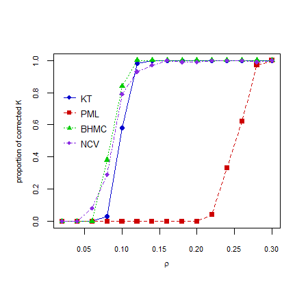
(a) $n=300$ and $\pi=(1/3,1/3,1/3)$

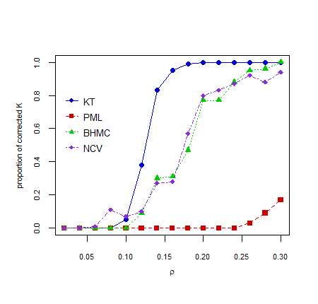
(b) $n=300$ and $\pi=(0.2,0.5,0.3)$

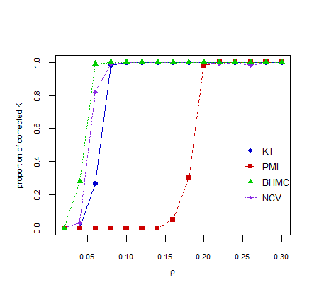
(c) $n=500$ and $\pi=(1/3,1/3,1/3)$

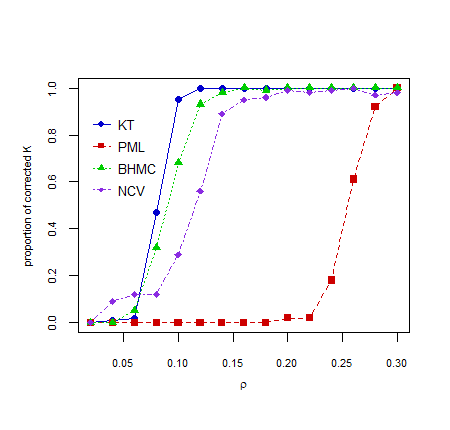
(d) $n=500$ and $\pi=(0.2,0.5,0.3)$

Figure 1: Proportion of correct estimates for $k_{0}$ using the methods: Krichevsky-Trofimov (KT), Beth-Hessian matrix with moment correction (BHMC), network cross-validation (NCV) and penalized maximum likelihood (PML). We consider the model with $k_{0}=3$, $P_{0}=\rho S_{0}$, where $S_{0}$ has diagonal entries equal to $2$ and off-diagonal entries equal to $1$. The tuning parameter in PML was chosen as $\lambda=0.1$ and in KT as $\epsilon=1$.

VI Discussion

In this paper we introduced a model selection procedure based on the Krichevsky-Trofimov mixture distribution for the number of communities in the Stochastic Block Model. We proved the almost sure convergence (strong consistency) of the penalized estimator (2) to the underlying number of communities, without assuming a known upper bound on that quantity. To our knowledge this is the first strong consistency result for an estimator of the number of communities. Moreover, it is the first unbounded estimator in the sense that the set of candidate values is allowed to grow with the sample size.

Our proposed penalty function (8) is of order $k^{3}\log n$, where $n$ is the number of nodes in the network, therefore for large $n$ it is considerably smaller than the $k(k+1)n\log n/2$ penalty term used in [17]. Even if we relate in Proposition 1 both objective functions, it is not evident how to derive the consistency of the BIC as considered in [17] with a smaller penalty term as the one we propose here. It also remains as an open question if the usual BIC penalty term that in this case would be $k(k+1)\log n$ leads to a consistent estimator of the number of communities, or if the KT criterion can be consistent excluding completely the penalty term, as in the case of context tree models, see [24]. From the point of view of the different degree regimes, in comparison to [17] we consider a wider family of sparse models with edge probability of order $\rho_{n}$, where $\rho_{n}$ can decrease to 0 at a rate such that $n\rho_{n}\rightarrow\infty$. It remains as an open question if it is even possible to obtain consistency for the number of communities in the sparse regime with $\rho_{n}=1/n$.

Appendix A Proofs of auxiliary results

We begin by stating without proof a basic inequality for the Gamma function. The proof of this result can be found in [28].

Lemma 9.

For integers $n=n_{1}+\cdots+n_{J}$ we have that

$$\dfrac{\prod\limits_{j=1}^{J}\left(\frac{n_{j}}{n}\right)^{n_{j}}}{\prod\limits_{j=1}^{J}\Gamma\left(n_{j}+\frac{1}{2}\right)}\;\leq\;\dfrac{1}{\Gamma\left(n+\frac{1}{2}\right)\Gamma\left(\frac{1}{2}\right)^{J-1}}\,.$$ (33)

We now follow by presenting the proof a Proposition 1.

Proof of Proposition 1.

To prove the first inequality observe that by definition of the KT distribution we have that

$$\begin{split}\textup{KT}_{k}(\mathbb{a}_{n\times n})&=\mathbb{E}_{\nu_{k}}[\,\mathbb{P}_{\pi,P}(\mathbb{a}_{n\times n})\,]\\ &\leq\mathbb{E}_{\nu_{k}}\Bigl{[}\,\sup_{(\pi,P)\in\Theta^{k}}\mathbb{P}_{\pi,P}(\mathbb{a}_{n\times n})\,\Bigr{]}\\ &=\sup_{(\pi,P)\in\Theta^{k}}\mathbb{P}_{\pi,P}(\mathbb{a}_{n\times n})\,.\end{split}$$

The second inequality is based on [26, Appendix I] and [25, Lemma 3.4]. For $(\pi,P)\in\Theta^{k}$ we have that

$$\mathbb{P}_{\pi,P}(\mathbb{z}_{n})\;=\;\prod\limits_{1\leq a\leq k}\pi_{a}^{n_{a}}$$ (34)

and

$$\mathbb{P}_{\pi,P}(\mathbb{a}_{n\times n}|\mathbb{z}_{n})\;=\;\prod\limits_{1\leq a\leq b\leq k}P_{a,b}^{o_{a,b}}(1-P_{a,b})^{n_{a,b}-o_{a,b}}\,.$$ (35)

Using that the maximum likelihood estimators for $\pi_{a}$ and $P_{a,b}$ are given by $\dfrac{n_{a}}{n}$ and $\dfrac{o_{a,b}}{n_{a,b}}$ respectively, we can bound above (34) and (35) by

$$\mathbb{P}_{\pi,P}(\mathbb{z}_{n})\;\leq\;\sup\limits_{(\pi,P)\in\Theta^{k}}\mathbb{P}_{\pi,P}(\mathbb{z}_{n})\;=\;\prod\limits_{1\leq a\leq k}\left(\dfrac{n_{a}}{n}\right)^{n_{a}}$$ (36)

and

$$\mathbb{P}_{\pi,P}(\mathbb{a}_{n\times n}|\mathbb{z}_{n}) \leq\sup\limits_{(\pi,P)\in\Theta^{k}}\mathbb{P}_{\pi,P}(\mathbb{a}_{n\times n}|\mathbb{z}_{n})$$

$$=\;\prod\limits_{1\leq a\leq b\leq k}\left(\dfrac{o_{a,b}}{n_{a,b}}\right)^{o_{a,b}}\left(1-\dfrac{o_{a,b}}{n_{a,b}}\right)^{n_{a,b}-o_{a,b}}.$$ (37)

Observe that the Krichevsky-Trofimov mixture distribution defined in (4) can be written as

$$\textup{KT}_{k}(\mathbb{a}_{n\times n})$$

$$=\sum\limits_{\mathbb{z}_{n}\in[k]^{n}}\scalebox{0.9}{$\biggl{(}\int_{\Theta^{k}_{1}}\mathbb{P}_{\pi,P}(\mathbb{z}_{n})\nu_{k}^{1}(\pi)d\pi\biggr{)}\biggl{(}\int_{\Theta^{k}_{2}}\mathbb{P}_{\pi,P}(\mathbb{a}_{n\times n}|\mathbb{z}_{n})\nu_{k}^{2}(P)dP\biggr{)}$}$$

$$=\sum\limits_{\mathbb{z}_{n}\in[k]^{n}}\textup{KT}_{k}(\mathbb{z}_{n})\textup{KT}_{k}(\mathbb{a}_{n\times n}|\mathbb{z}_{n})\,,$$ (38)

where

$$\ \nu^{1}_{k}(\pi)=\dfrac{\Gamma(\frac{k}{2})}{\Gamma(\frac{1}{2})^{k}}\prod\limits_{1\leq a\leq k}\pi_{a}^{-1/2}\,,$$

$$\quad\nu^{2}_{k}(P)=\prod_{1\leq a\leq b\leq k}\dfrac{1}{\Gamma(\frac{1}{2})^{2}}P_{a,b}^{-1/2}(1-P_{a,b})^{-1/2}\,,$$

$$\Theta^{k}_{1}=\{\,\pi\,|\,\pi\in(0,1]^{k},\sum\limits_{a=1}^{k}\pi_{a}=1\}\,,$$

and

$$\Theta^{k}_{2}=\{\,P\,|\,P\in[0,1]^{k\times k},P\text{ is symmetric}\,\}.$$

We start with the evaluation of $\textup{KT}_{k}(\mathbb{z}_{n})$. By a simple calculation we have that

$$\begin{split}\textup{KT}_{k}(\mathbb{z}_{n})&\;=\;\dfrac{\Gamma\left(\frac{k}{2}\right)}{\Gamma\left(\frac{1}{2}\right)^{k}}\;\dfrac{\prod_{a=1}^{k}\Gamma\left(n_{a}+\frac{1}{2}\right)}{\Gamma\left(n+\frac{k}{2}\right)}\,.\end{split}$$ (39)

Then combining (36) and (39) we obtain the bound

$$\dfrac{\mathbb{P}_{\pi,P}(\mathbb{z}_{n})}{\textup{KT}_{k}(\mathbb{z}_{n})}\;\leq\;\dfrac{\Gamma\left(\frac{1}{2}\right)^{k}\Gamma\left(n+\frac{k}{2}\right)}{\Gamma\left(\frac{k}{2}\right)}\;\prod\limits_{1\leq a\leq k}\dfrac{\left(\dfrac{n_{a}}{n}\right)^{n_{a}}}{\Gamma\left(n_{a}+\frac{1}{2}\right)}\,.$$ (40)

Using the fact that $n_{1}+\cdots+n_{k}=n$ and Lemma 9 we can bound the second factor in the right-hand side of the last inequality by

$$\prod\limits_{1\leq a\leq k}\dfrac{\left(\dfrac{n_{a}}{n}\right)^{n_{a}}}{\Gamma\left(n_{a}+\frac{1}{2}\right)}\;\leq\;\dfrac{1}{\Gamma\left(\frac{1}{2}\right)^{k-1}\,\Gamma\left(n+\frac{1}{2}\right)}$$

and then we obtain the bound

$$\dfrac{\mathbb{P}_{\pi,P}(\mathbb{z}_{n})}{\textup{KT}_{k}(\mathbb{z}_{n})}\;\leq\;\dfrac{\Gamma\left(\frac{1}{2}\right)\Gamma\left(n+\frac{k}{2}\right)}{\Gamma\left(\frac{k}{2}\right)\Gamma\left(n+\frac{1}{2}\right)}\,.$$ (41)

The same arguments above can be used to derive the equality

$$\textup{KT}_{k}(\mathbb{a}_{n\times n}|\mathbb{z}_{n})=\prod_{1\leq a\leq b\leq k}\;\dfrac{\Gamma\left(o_{a,b}+\frac{1}{2}\right)\Gamma\left(n_{a,b}-o_{a,b}+\frac{1}{2}\right)}{\Gamma\left(\frac{1}{2}\right)^{2}\Gamma\left(n_{a,b}+1\right)}$$

and the upper bound

$$\begin{split}\dfrac{\mathbb{P}_{\pi,P}(\mathbb{a}_{n\times n}|\mathbb{z}_{n})}{\textup{KT}_{k}(\mathbb{a}_{n\times n}|\mathbb{z}_{n})}&\;\leq\;\prod\limits_{1\leq a\leq b\leq k}\,\dfrac{\Gamma\left(\textstyle\frac{1}{2}\right)\Gamma\left(n_{a,b}+1\right)}{\Gamma\left(n_{a,b}+\frac{1}{2}\right)}\,.\end{split}$$ (42)

Then combining the bounds in (41) and (42) we have that

$$\dfrac{\mathbb{P}_{\pi,P}(\mathbb{z}_{n},\mathbb{a}_{n\times n})}{\textup{KT}_{k}(\mathbb{z}_{n},\mathbb{a}_{n\times n})}\;\leq\;e^{C(\mathbb{z}_{n},\mathbb{a}_{n\times n})}\,,$$ (43)

where

$$C(\mathbb{z}_{n},\mathbb{a}_{n\times n})\;= \;\log\Bigl{(}\frac{\Gamma\left(\frac{1}{2}\right)\Gamma\left(n+\frac{k}{2}\right)}{\Gamma\left(\frac{k}{2}\right)\Gamma\left(n+\frac{1}{2}\right)}\Bigr{)}$$

$$+\sum\limits_{1\leq a\leq b\leq k}\log\Bigl{(}\frac{\Gamma\left(\frac{1}{2}\right)\Gamma\left(n_{a,b}+1\right)}{\Gamma\left(n_{a,b}+\frac{1}{2}\right)}\Bigr{)}\,.$$ (44)

It can be shown, by using Stirlings’ formula for the $\Gamma$ function

$$x^{x-\frac{1}{2}}e^{-x}\sqrt{2\pi}\;\leq\;\Gamma(x)\;\leq\;x^{x-\frac{1}{2}}e^{-x}\sqrt{2\pi}e^{\frac{1}{12x}}$$

as in [26, Appendix I], that

$$\begin{split}\scalebox{0.95}{$\log\left(\frac{\Gamma\left(\frac{1}{2}\right)\Gamma\left(n+\frac{k}{2}\right)}{\Gamma\left(\frac{k}{2}\right)\Gamma\left(n+\frac{1}{2}\right)}\right)$}&\scalebox{0.95}{$\;\leq\;\left(\frac{k-1}{2}\right)\log n+\frac{k(k-1)}{4n}+\frac{1}{12n}+\log\frac{\Gamma(\frac{1}{2})}{\Gamma(\frac{k}{2})}$}\\ &\scalebox{0.95}{$\;\leq\;\left(\frac{k-1}{2}\right)\log n+\frac{k(k-1)}{4n}+1$}\end{split}$$ (45)

and for $1\leq a\leq b\leq k$,

$$\begin{split}\scalebox{0.95}{$\log\left(\frac{\Gamma\left(\frac{1}{2}\right)\Gamma\left(n_{a,b}+1\right)}{\Gamma\left(n_{a,b}+\frac{1}{2}\right)}\right)$}&\;\scalebox{0.95}{$\leq\;\frac{1}{2}\log n_{a,b}+\frac{1}{2n_{a,b}}+\frac{1}{12n_{a,b}}+\log\Gamma(\frac{1}{2})$}\\ &\scalebox{0.95}{$\;\leq\;\log n+\frac{3}{2}$}\end{split}$$ (46)

where the last inequality follows from the fact that $n_{a,b}\leq n^{2}$ for all $a$ and $b$. Summing the bounds (45) and (46) we obtain in (A) that

$$C(\mathbb{z}_{n},\mathbb{a}_{n\times n})\;\leq\;\textstyle\frac{k(k+2)-1}{2}\log n+c_{k}\,,$$ (47)

where

$$c_{k}=k(k+1)+1\,.$$

Using the uniform bound (47) and (43) we can finally write

$$\begin{split}&\scalebox{0.95}{$\log\sup\limits_{(\pi,P)\in\Theta^{k}}\mathbb{P}_{\pi,P}(\mathbb{a}_{n\times n})\,\;$}\\ &\scalebox{0.95}{$\leq\sup\limits_{(\pi,P)\in\Theta^{k}}\log\biggl{(}\;\sum\limits_{\mathbb{z}_{n}\in[k]^{n}}e^{C(\mathbb{z}_{n},\mathbb{a}_{n\times n})}\textup{KT}_{k}(\mathbb{z}_{n})\textup{KT}_{k}(\mathbb{a}_{n\times n}|\mathbb{z}_{n})\biggr{)}$}\\ &\leq\log\textup{KT}_{k}(\mathbb{a}_{n\times n})+\textstyle\frac{k(k+2)-1}{2}\log n+c_{k}\end{split}$$

and this concludes the proof. ∎

Now we state and prove a lemma that is useful to bound the probability of overestimation.

Lemma 10.

For $k>k_{0}$ we have

$$\begin{split}&\mathbb{P}_{\pi^{0},P^{0}}(\hat{k}_{\mbox{\tiny{KT}}}(\mathbb{a}_{n\times n})=k)\\ &\hskip 56.9055pt\;\leq\;\exp\left\{\textstyle\frac{k_{0}(k_{0}+2)-1}{2}\log n+c_{k_{0}}+d_{k_{0},k,n}\right\}\,,\end{split}$$

where $d_{k_{0},k,n}=\mbox{pen}(k_{0},n)-\mbox{pen}(k,n)$.

Proof.

For $k>k_{0}$ define the events

$$A(k)\;=\;\Bigl{\{}\operatorname*{arg\,max}\limits_{1\leq k^{\prime}\leq n}\{\,\log\mbox{KT}_{k^{\prime}}(\mathbb{a}_{n\times n})-\frac{1}{2}(k^{\prime})^{3}\log n\,\}=k\Bigr{\}}$$

and

$$B(k)\;=\;\Bigl{\{}\mbox{KT}_{k_{0}}(\mathbb{a}_{n\times n})\leq\mbox{KT}_{k}(\mathbb{a}_{n\times n})\text{e}^{d_{k_{0},k,n}}\Bigr{\}}\,,$$

where

$$d_{k_{0},k,n}=\mbox{pen}(k_{0},n)-\mbox{pen}(k,n)\,.$$

Observe that $A(k)\subset B(k)$ for all $k$. Then

$$\mathbb{P}_{\pi^{0},P^{0}}(\hat{k}_{\mbox{\tiny{KT}}}(\mathbb{a}_{n\times n})=k)\; =\;\sum\limits_{\mathbb{a}_{n\times n}}\mathbb{P}_{\pi^{0},P^{0}}(\mathbb{a}_{n\times n})\mathds{1}_{A(k)}$$

$$\leq\;\sum\limits_{\mathbb{a}_{n\times n}}\mathbb{P}_{\pi^{0},P^{0}}(\mathbb{a}_{n\times n})\mathds{1}_{B(k)}\,.$$ (48)

By Proposition 1

and therefore

$$\mathbb{P}_{\pi^{0},P^{0}}(\mathbb{a}_{n\times n})\;\leq\;\mbox{KT}_{k_{0}}(\mathbb{a}_{n\times n})n^{\frac{k_{0}(k_{0}+2)-1}{2}}e^{c_{k_{0}}}\,.$$ (49)

Applying (49) in (A) we obtain that

$$\mathbb{P}_{\pi^{0},P^{0}}(\hat{k}_{\mbox{\tiny{KT}}} (\mathbb{a}_{n\times n})=k)$$

$$\;\leq\;\sum\limits_{\mathbb{a}_{n\times n}}\mbox{KT}_{k_{0}}(\mathbb{a}_{n\times n})n^{\frac{k_{0}(k_{0}+2)-1}{2}}e^{c_{k_{0}}}\mathds{1}_{B(k)}$$

$$\;\leq\;\sum\limits_{\mathbb{a}_{n\times n}}\mbox{KT}_{k}(\mathbb{a}_{n\times n})\,e^{d_{k_{0},k,n}}n^{\frac{k_{0}(k_{0}+2)-1}{2}}e^{c_{k_{0}}}$$

$$=\exp\left\{\textstyle\frac{k_{0}(k_{0}+2)-1}{2}\log n+c_{k_{0}}+d_{k_{0},k,n}\right\}\,,$$

where the last equality follows from the fact that $\textup{KT}_{k}(\cdot)$ is a probability distribution on the space of adjacency matrices. This concludes the proof of Lemma 10. ∎

Andressa Cerqueira received a PhD degree in Statistics from the University of São Paulo in 2018. During 2018 she was a postdoctoral researcher at University of Campinas. During 2019 she spent one year as a visiting postdoctoral researcher at University of Michigan. Since 2020 she is Assistant Professor at Department of Statistics at Federal University of São Carlos (UFSCar) and her research is focused on inference in networks.

Florencia Leonardi received a bachelor’s degree in Mathematics from the University of Mar del Plata in 2002 and a PhD degree in Bioinformatics from the University of São Paulo in 2007. She became Adjoint Professor in 2008 at the Institute of Mathematics and Statistics of the University of São Paulo, and Associate Professor since 2017. During 2014- 2015 she spent a sabbatical year as a Visiting Professor at ETHZ in Switzerland. Her main research interests are inference and applications of stochastic processes.

References

• [1] P. W. Holland, K. B. Laskey, and S. Leinhardt, “Stochastic blockmodels: First steps,” Social networks, vol. 5, no. 2, pp. 109–137, 1983.
• [2] P. J. Bickel and A. Chen, “A nonparametric view of network models and newman–girvan and other modularities,” Proceedings of the National Academy of Sciences, vol. 106, no. 50, pp. 21 068–21 073, 2009.
• [3] A. A. Amini, A. Chen, P. J. Bickel, and E. Levina, “Pseudo-likelihood methods for community detection in large sparse networks,” The Annals of Statistics, vol. 41, no. 4, pp. 2097–2122, 2013.
• [4] J.-J. Daudin, F. Picard, and S. Robin, “A mixture model for random graphs,” Statistics and computing, vol. 18, no. 2, pp. 173–183, 2008.
• [5] P. Latouche, E. Birmele, and C. Ambroise, “Variational bayesian inference and complexity control for stochastic block models,” Statistical Modelling, vol. 12, no. 1, pp. 93–115, 2012.
• [6] K. Rohe, S. Chatterjee, B. Yu et al., “Spectral clustering and the high-dimensional stochastic blockmodel,” The Annals of Statistics, vol. 39, no. 4, pp. 1878–1915, 2011.
• [7] S. L. van der Pas and A. W. van der Vaart, “Bayesian community detection,” Bayesian Analysis, vol. 13, no. 3, pp. 767–796, 2018.
• [8] P. Bickel, D. Choi, X. Chang, and H. Zhang, “Asymptotic normality of maximum likelihood and its variational approximation for stochastic blockmodels,” Ann. Statist., vol. 41, no. 4, pp. 1922–1943, 2013.
• [9] L. Su, W. Wang, and Y. Zhang, “Strong consistency of spectral clustering for stochastic block models,” IEEE Transactions on Information Theory, vol. 66, no. 1, pp. 324–338, 2019.
• [10] E. Abbe, “Community detection and stochastic block models: recent developments,” The Journal of Machine Learning Research, vol. 18, no. 1, pp. 6446–6531, 2017.
• [11] C. M. Le and E. Levina, “Estimating the number of communities in networks by spectral methods,” arXiv preprint arXiv:1507.00827, 2015.
• [12] P. J. Bickel and P. Sarkar, “Hypothesis testing for automated community detection in networks,” Journal of the Royal Statistical Society: Series B (Statistical Methodology), vol. 78, no. 1, pp. 253–273, 2016.
• [13] J. Lei, “A goodness-of-fit test for stochastic block models,” The Annals of Statistics, vol. 44, no. 1, pp. 401–424, 2016.
• [14] K. Chen and J. Lei, “Network cross-validation for determining the number of communities in network data,” Journal of the American Statistical Association, vol. 113, no. 521, pp. 241–251, 2018.
• [15] T. Li, E. Levina, and J. Zhu, “Network cross-validation by edge sampling,” Biometrika, vol. 107, no. 2, pp. 257–276, 2020.
• [16] C. Biernacki, G. Celeux, and G. Govaert, “Assessing a mixture model for clustering with the integrated completed likelihood,” IEEE Transactions on Pattern Analysis and Machine Intelligence, vol. 22, no. 7, pp. 719–725, July 2000.
• [17] Y. R. Wang and P. J. Bickel, “Likelihood-based model selection for stochastic block models,” The Annals of Statistics, vol. 45, no. 2, pp. 500–528, 2017.
• [18] G. Schwarz, “Estimating the dimension of a model,” Ann. Statist., vol. 6, no. 2, pp. 461–464, 1978.
• [19] J. Hu, H. Qin, T. Yan, and Y. Zhao, “Corrected bayesian information criterion for stochastic block models,” Journal of the American Statistical Association, vol. 0, no. 0, pp. 1–13, 2019.
• [20] A. Barron, J. Rissanen, and Bin Yu, “The minimum description length principle in coding and modeling,” IEEE Transactions on Information Theory, vol. 44, no. 6, pp. 2743–2760, Oct 1998.
• [21] R. E. Krichevsky and V. K. Trofimov, “The performance of universal encoding.” IEEE Transactions on Information Theory, vol. 27, no. 2, pp. 199–206, 1981.
• [22] L. Finesso, H. Kimura, and S. Kodama, “Estimation of the order of a finite markov chain,” in Recent Advances in the Mathematical Theory of Systems, Control, and Network Signals, Proc. MTNS-91, H. Kimura and S. Kodama, Eds., Mita Press, 1992, pp. 643–645.
• [23] I. Csiszár and P. C. Shields, “The consistency of the bic markov order estimator,” The Annals of Statistics, vol. 28, no. 6, pp. 1601–1619, 2000.
• [24] I. Csiszar and Z. Talata, “Context tree estimation for not necessarily finite memory processes, via bic and mdl,” IEEE Transactions on Information Theory, vol. 52, no. 3, pp. 1007–1016, March 2006.
• [25] C.-C. Liu and P. Narayan, “Order estimation and sequential universal data compression of a hidden markov source by the method of mixtures,” IEEE Transactions on Information Theory, vol. 40, no. 4, pp. 1167–1180, 1994.
• [26] E. Gassiat and S. Boucheron, “Optimal error exponents in hidden markov models order estimation,” IEEE Transactions on Information Theory, vol. 49, no. 4, pp. 964–980, 2003.
• [27] Y. Zhao, E. Levina, and J. Zhu, “Consistency of community detection in networks under degree-corrected stochastic block models,” The Annals of Statistics, vol. 40, no. 4, pp. 2266–2292, 2012.
• [28] L. Davisson, R. McEliece, M. Pursley, and M. Wallace, “Efficient universal noiseless source codes,” IEEE Transactions on Information Theory, vol. 27, no. 3, pp. 269–279, 1981.