ABSTRACT

The cosmological principle is one of the cornerstones in modern cosmology. It assumes that the universe is homogeneous and isotropic on cosmic scales. Both the homogeneity and the isotropy of the universe should be tested carefully. In the present work, we are interested in probing the possible preferred direction in the distribution of type Ia supernovae (SNIa). To our best knowledge, two main methods have been used in almost all of the relevant works in the literature, namely the hemisphere comparison (HC) method and the dipole fitting (DF) method. However, the results from these two methods are not always approximately coincident with each other. In this work, we test the cosmic anisotropy by using these two methods with the Joint Light-Curve Analysis (JLA) and simulated SNIa datasets. In many cases, both methods work well, and their results are consistent with each other. However, in the cases with two (or even more) preferred directions, the DF method fails while the HC method still works well. This might shed new light on our understanding of these two methods.

Testing the Cosmic Anisotropy with Supernovae Data: Hemisphere Comparison and Dipole Fitting

I Introduction

As is well known, the cosmological principle is one of the cornerstones in modern cosmology Weinberg:cos ; Kolb90 . It assumes that the universe is homogeneous and isotropic on cosmic scales. In fact, the cosmological principle has been observed to be approximately valid across a very large part of the universe (e.g. Hogg:2004vw ; Hajian:2006ud ). However, it is not born to be true, and this assumption should be strictly tested by using the cosmological observations. As its two main parts, both the homogeneity and the isotropy of the universe should be probed carefully.

In fact, the cosmological principle has not yet been well proven on cosmic scales $\lower 3.22916pt\hbox{$\sim$}\hbox to0.0pt{\hss\raise 1.1625pt\hbox{$>$}}\,1\,$Gpc Caldwell:2007yu . On the other hand, the local universe is obviously inhomogeneous and anisotropic on small scales. In particular, the nearby sample has been examined for evidence of a local “Hubble Bubble” Zehavi:1998gz . If the cosmological principle can be relaxed, it is possible to explain the apparent cosmic acceleration discovered in 1998 Riess:1998cb ; Perlmutter:1998np , without invoking dark energy DE or modified gravity MG . For instance, giving up the cosmic homogeneity, it is reasonable to imagine that we are living in a locally underdense void. One of such models is the well-known Lemaître-Tolman-Bondi (LTB) void model LTB ; Goode:1982pg ; Alnes:2005rw ; GarciaBellido:2008nz ; Enqvist:2006cg ; Celerier:2012xr ; Ishak:2013vha ; Clifton:2008hv ; Zhang:2012qr ; Yan:2014eca . In this model, the universe is spherically symmetric and radially inhomogeneous, and we are living in a locally underdense void centered nearby our location. The Hubble diagram inferred from lines-of-sight originating at the center of the void might be misinterpreted to indicate cosmic acceleration Alnes:2005rw ; GarciaBellido:2008nz ; Enqvist:2006cg ; Celerier:2012xr ; Ishak:2013vha ; Clifton:2008hv ; Zhang:2012qr ; Yan:2014eca . In fact, the LTB-like models violating the cosmological principle have been extensively considered in the literature nowadays.

In the literature, the cosmic homogeneity has been tested by using e.g. type Ia supernovae (SNIa) Celerier:1999hp ; Clifton:2008hv ; Celerier:2012xr , cosmic microwave background (CMB) Caldwell:2007yu ; Moffat:2005yx ; Alnes:2006pf ; Clifton:2009kx ; Clarkson:2010ej ; Moss:2010jx , time drift of cosmological redshifts Uzan:2008qp ; Quartin:2009xr , baryon acoustic oscillations (BAO) Bolejko:2008cm ; February:2012fp ; Zibin:2008vk , integrated Sachs-Wolfe effect Tomita:2009wz , galaxy surveys Labini:2010qx , kinetic Sunyaev Zel’dovich effect Zhang:2010fa ; Valkenburg:2012td ; Bull:2011wi ; Moss:2011ze ; Marra:2011ct , ages of old high-redshift objects Yan:2014eca , observational $H(z)$ data Zhang:2012qr , and growth of large-scale structure Celerier:2012xr . However, the debate on the inhomogeneous universe has not been settled by now.

In contrast to the LTB-like models giving up the cosmic homogeneity, there is another kind of models violating the cosmological principle, in which the universe is not isotropic. For example, the well-known Gödel solution Godel:1949ga of the Einstein field equations describes a homogeneous rotating universe. Although the Gödel universe has some exotic features (see e.g. Li:2016nnn ), it is indeed an interesting idea that our universe is rotating around an axis. In fact, this idea can be completely independent of the Gödel universe. In addition, there are other kinds of anisotropic models in the literature. For instance, most of the well-known Bianchi type I $\sim$ IX universes Bianchi ; Mishra:2015jja are anisotropic in general.

In fact, some hints of the cosmic anisotropy have been claimed in the literature. For example, it is found that there exists a preferred direction in the CMB temperature map (known as the “Axis of Evil” in the literature) Axisofevil ; Zhao:2016fas ; Hansen:2004vq , the distribution of SNIa Schwarz:2007wf ; Antoniou:2010gw ; Mariano:2012wx ; Cai:2011xs ; Zhao:2013yaa ; Yang:2013gea ; Chang:2014nca ; Lin:2015rza ; Chang:2017bbi ; Javanmardi:2015sfa ; Bengaly:2015dza , gamma-ray bursts (GRBs) Meszaros:2009ux ; Wang:2014vqa ; Chang:2014jza , rotationally supported galaxies Zhou:2017lwy ; Chang:2018vxs , quasars and radio galaxies Singal:2013aga ; Bengaly:2017slg , and the quasar optical polarization data Hutsemekers ; Pelgrims:2016mhx . In addition, using the absorption systems in the spectra of distant quasars, it is claimed that the fine structure “constant” $\alpha$ is not only time-varying Webb98 ; Webb00 (see also e.g. Uzan10 ; Barrow09 ; HWalpha ), but also spatially varying King:2012id ; Webb:2010hc . Precisely speaking, there is also a preferred direction in the data of $\Delta\alpha/\alpha$. It is found in Mariano:2012wx that the preferred direction in $\Delta\alpha/\alpha$ might be correlated with the one in the distribution of SNIa. Up to date, the hints of the cosmic anisotropy are still accumulating.

In the present work, we are interested in probing the possible preferred direction in the distribution of SNIa Schwarz:2007wf ; Antoniou:2010gw ; Mariano:2012wx ; Cai:2011xs ; Zhao:2013yaa ; Yang:2013gea ; Chang:2014nca ; Lin:2015rza ; Chang:2017bbi . To our best knowledge, two main methods have been used in almost all of the relevant works in the literature (e.g. Schwarz:2007wf ; Antoniou:2010gw ; Mariano:2012wx ; Cai:2011xs ; Zhao:2013yaa ; Yang:2013gea ; Chang:2014nca ; Lin:2015rza ; Chang:2017bbi ), namely the hemisphere comparison (HC) method proposed in Schwarz:2007wf and then improved by Antoniou:2010gw (see also e.g. Cai:2011xs ; Yang:2013gea ; Chang:2014nca ), and the dipole fitting (DF) method proposed in Mariano:2012wx (see also e.g. Chang:2014nca ; Lin:2015rza ; Chang:2017bbi ; Zhou:2017lwy ; Chang:2018vxs ; Yang:2013gea ; Wang:2014vqa ). In the HC method, the data points are randomly divided into many pairs of hemispheres according to their positions in the sky, and then these pairs of hemispheres are compared until the preferred direction with a maximum anisotropy level is found. In the DF method, the data points are directly fitted to a dipole (or dipole plus monopole in some cases). We refer to the next sections for the details of these two methods.

It is natural to expect that the preferred directions found by these two methods are approximately coincident with each other. Of course, in many cases the answer is “yes”. However, it is not always “yes” unfortunately. For example, the preferred direction in the Union2 SNIa dataset found by the DF method is approximately opposite to the one found by the HC method Chang:2014nca . On the other hand, a preferred direction in the Union2.1 SNIa dataset was found by the DF method, but there is a null signal for the HC method Yang:2013gea . In addition, the DF method failed to find the preferred direction in the JLA SNIa dataset Lin:2015rza ; Chang:2017bbi . To our best knowledge, the HC method has not been used to find the preferred direction in the JLA SNIa dataset up to now, and hence we do this in the present work. In contrast to the failure of the DF method Lin:2015rza ; Chang:2017bbi , the HC method works well in the JLA SNIa dataset (see below). Therefore, it is of interest to compare these two methods carefully, and we will do this by using several simulated SNIa datasets. In fact, this might shed new light on our understanding of these two methods.

The rest of this paper is organized as follows. In Sec. II, we briefly review the key points of the HC method and the DF method, and then we use them to find the possible preferred direction in the JLA SNIa dataset. In Sec. III, we compare these two methods by using several simulated SNIa datasets. In Sec. IV, some brief concluding remarks are given.

II The preferred direction in the JLA SNIa dataset

As mentioned above, to our best knowledge, the HC method has not been used to find the preferred direction in the JLA dataset consisting of 740 SNIa Betoule:2014frx up to now. We will do this here. At first, we briefly review the key points of the HC method following Antoniou:2010gw . Its goal is to identify the direction of the axis of maximal asymmetry for the corresponding dataset. Usually, the physical quantity to be compared is the accelerating expansion rate, namely the deceleration parameter $q_{0}$ Weinberg:cos ; Kolb90 (note that $q_{0}<0$ means that the universe is accelerating). As is well known, in the spatially flat $\Lambda$CDM model, the deceleration parameter $q_{0}$ is related to the fractional density of the pressureless matter $\Omega_{m0}$ according to $q_{0}=-1+3\Omega_{m0}/2$. So, it is convenient to use $\Omega_{m0}$ instead Antoniou:2010gw , as we consider the spatially flat $\Lambda$CDM model throughout this work. Following Antoniou:2010gw , the main steps to implement the HC method are (i) Generate a random direction $\hat{r}_{\rm rnd}$ indicated by $(l,\,b)$ with a uniform probability distribution, where $l\in[\,0^{\circ},\,360^{\circ})$ and $b\in[-90^{\circ},\,+90^{\circ}\,]$ are the longitude and the latitude in the galactic coordinate system, respectively. (ii) Split the dataset under consideration into two subsets according to the sign of the inner product $\hat{r}_{\rm rnd}\cdot\hat{r}_{\rm dat}$, where $\hat{r}_{\rm dat}$ is a unit vector describing the direction of each SNIa in the dataset. Thus, one subset corresponds to the hemisphere in the direction of the random vector (defined as “up”), while the other subset corresponds to the opposite hemisphere (defined as “down”). Noting that the position of each SNIa in the dataset is usually given by right ascension (ra) and declination (dec) in degree (equatorial coordinate system, J2000), one should convert $\hat{r}_{\rm rnd}$ and $\hat{r}_{\rm dat}$ to Cartesian coordinates in this step. (iii) Find the best-fit values on $\Omega_{m0}$ in each hemisphere ($\Omega_{m0,u}$ and $\Omega_{m0,d}$), and then obtain the so-called anisotropy level (AL) quantified through the normalized difference Antoniou:2010gw ,

$${\rm AL}\equiv\frac{\Delta\Omega_{m0}}{\bar{\Omega}_{m0}}=2\cdot\frac{\Omega_{m0,u}-\Omega_{m0,d}}{\Omega_{m0,u}+\Omega_{m0,d}}\,.$$ (1)

(iv) Repeat for $N$ random directions $\hat{r}_{\rm rnd}$ and find the maximum AL, as well as the corresponding direction of maximum anisotropy. (v) Obtain the $1\sigma$ error $\sigma_{\rm AL}$ associated with the maximum AL Antoniou:2010gw ,

$$\sigma_{\rm AL}=\frac{\sqrt{\sigma_{\Omega_{m0,u}^{\rm max}}^{2}+\sigma_{\Omega_{m0,d}^{\rm max}}^{2}}}{\Omega_{m0,u}^{\rm max}+\Omega_{m0,d}^{\rm max}}\,.$$ (2)

Note in Antoniou:2010gw that $\sigma_{\rm AL}$ is the error due to the uncertainties of the SNIa distance moduli propagated to the best-fit $\Omega_{m0}$ on each hemisphere and thus to AL. One can identify all the test axes corresponding to an AL within $1\sigma$ from the maximum AL, namely ${\rm AL=AL}_{\rm max}\pm\sigma_{\rm AL}$. These axes cover an angular region corresponding to the $1\sigma$ range of the maximum anisotropy direction. We refer to Antoniou:2010gw for more details of the HC method.

In many of the relevant works following Antoniou:2010gw , Mathematica was commonly used, and the number of random directions in step (iv) are taken to be approximately equal to the number of data points as suggested by Antoniou:2010gw . In this work, we use Matlab instead, and the number of random directions in step (iv) can be $N\sim{\cal O}(10^{4})$ or even more.

Here, we implement the HC method to the JLA dataset consisting of 740 SNIa Betoule:2014frx . We first repeat 10000 random directions $(l,\,b)$ across the whole sky, and find that the directions with the largest ALs concentrate around two directions, namely $(300.6575^{\circ},\,28.1678^{\circ})$ and $(23.4274^{\circ},\,1.7021^{\circ})$. Then, we densely repeat $5000\sim 20000$ random directions from the Gaussian distributions with the means in these two preliminary directions, respectively. Finally, we find that the $1\sigma$ angular region with the maximum AL is in the direction

$$(l,\,b)\,_{\rm HC,\,max}^{\rm JLA}=({23.4893^{\circ}}\,^{+21.6274^{\circ}}_{-12.8318^{\circ}}\,,\,{2.2524^{\circ}}\,^{+3.7961^{\circ}}_{-22.6837^{\circ}})\,,$$ (3)

and the corresponding maximum AL (with $1\sigma$ uncertainty) is

$${\rm AL_{max}^{JLA}}=0.3132\pm 0.1003\,.$$ (4)

In addition, we also find a sub-maximum AL in the direction (with $1\sigma$ uncertainty)

$$(l,\,b)\,_{\rm HC,\,sub}^{\rm JLA}=({299.4711^{\circ}}\,^{+46.1314^{\circ}}_{-23.3855^{\circ}}\,,\,{28.3912^{\circ}}\,^{+6.5202^{\circ}}_{-17.0096^{\circ}})\,,$$ (5)

and the corresponding sub-maximum AL (with $1\sigma$ uncertainty) is

$${\rm AL_{sub}^{JLA}}=0.2873\pm 0.1110\,.$$ (6)

In fact, it is not so rare to find two preferred directions (see e.g. Zhou:2017lwy ). Note that the second preferred direction given in Eq. (5) is consistent with the one $(l,\,b)=(309^{\circ},\,18^{\circ})$ found in Antoniou:2010gw for the Union2 SNIa dataset within the $1\sigma$ region. We present the pseudo-color map of AL$(l,\,b)$ in Fig. 1. It is clear to see the two preferred directions within the red regions.

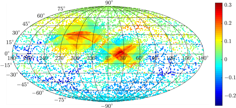
Figure 1: The pseudo-color map of AL$(l,\,b)$ obtained by using the HC method to the JLA SNIa dataset. The two preferred directions $(23.49^{\circ},\,2.25^{\circ})$ and $(299.47^{\circ},\,28.39^{\circ})$ are within the red regions. See the text for details.

Figure 2: The marginalized probability distributions of the dipole magnitude $A_{D}$ and the dipole direction $(l,\,b)$, obtained by using the DF method to the JLA SNIa dataset with the priors $\Omega_{m0}=0.295$ and $A_{D}\geq 0$. Note that $A_{D}$ is given in units of $10^{-3}$. See the text for details.

Next, let us turn to the DF method. It has already been known that the DF method failed to find the preferred direction in the JLA SNIa dataset Lin:2015rza ; Chang:2017bbi . But here we would like to generalize the main results. At first, we briefly review the key points of the DF method following e.g. Mariano:2012wx ; Chang:2014nca ; Lin:2015rza ; Chang:2017bbi ; Zhou:2017lwy ; Chang:2018vxs ; Yang:2013gea ; Wang:2014vqa . If the observational quantity under consideration is denoted by $\xi$, the corresponding $\chi^{2}$ is given by $\chi^{2}=(\vec{\xi}_{obs}-\vec{\xi}_{th})^{T}\,{\bf C}^{-1}(\vec{\xi}_{obs}-\vec{\xi}_{th})$, where $\bf C$ is the covariance matrix of $\vec{\xi}$. When $\bf C$ is a diagonal matrix, it reduces to $\chi^{2}=\sum(\xi_{obs,i}-\xi_{th,i})^{2}/\sigma_{\xi,i}^{2}\,$. If $\xi$ is anisotropic, one can consider a dipole plus monopole correction, namely $\xi_{th}=\bar{\xi}_{th}\left[\,1+B+A_{D}\left(\hat{n}\cdot\hat{p}\right)\,\right]$, where $B$ and $A_{D}$ are the monopole term and the dipole magnitude, respectively; $\hat{n}$ is the dipole direction; $\hat{p}$ is the unit 3-vector pointing toward the data point; $\bar{\xi}_{th}$ is the value predicted by the isotropic theoretical model. Usually, the monopole term $B$ is negligible, and one can only consider the dipole modulation, namely

$$\xi_{th}=\bar{\xi}_{th}\left[\,1+A_{D}\left(\hat{n}\cdot\hat{p}\right)\,\right].$$ (7)

In terms of the galactic coordinates $(l,\,b)$, the dipole direction is given by

$$\hat{n}=\cos(b)\cos(l)\,\hat{\bf i}+\cos(b)\sin(l)\,\hat{\bf j}+\sin(b)\,\hat{\bf k}\,,$$ (8)

where $\hat{\bf i}$, $\hat{\bf j}$, $\hat{\bf k}$ are the unit vectors along the axes of Cartesian coordinates system. The position of the $i$-th data point with the galactic coordinates $(l_{i},\,b_{i})$ is given by

$$\hat{p}_{i}=\cos(b_{i})\cos(l_{i})\,\hat{\bf i}+\cos(b_{i})\sin(l_{i})\,\hat{\bf j}+\sin(b_{i})\,\hat{\bf k}\,.$$ (9)

One can find the best-fit dipole direction $(l,\,b)$ and the dipole magnitude $A_{D}$ as well as the other model parameters by minimizing the corresponding $\chi^{2}$. Note that in practice $\xi$ can be various observational quantities, e.g. the distance modulus $\mu$ of SNIa or GRBs Mariano:2012wx ; Chang:2014nca ; Lin:2015rza ; Chang:2017bbi ; Yang:2013gea ; Wang:2014vqa , the centripetal acceleration $g_{\dagger}$ in the rotationally supported disk galaxies Zhou:2017lwy ; Chang:2018vxs , and the varying fine structure “constant” $\alpha$ Mariano:2012wx . We refer to e.g. Mariano:2012wx ; Chang:2014nca ; Lin:2015rza ; Chang:2017bbi ; Zhou:2017lwy ; Chang:2018vxs ; Yang:2013gea ; Wang:2014vqa for more details of the DF method.

In our case of the JLA SNIa dataset, $\xi$ in Eq. (7) is the distance modulus $\mu$ of SNIa. The theoretical $\bar{\mu}_{th}$ predicted by the isotropic flat $\Lambda$CDM model is given by Weinberg:cos ; Betoule:2014frx ; Lin:2015rza ; Chang:2017bbi ; Zou:2017ksd

$$\bar{\mu}_{th}=5\log_{10}\frac{d_{L}}{\rm Mpc}+25\,,$$ (10)

where the isotropic luminosity distance reads

$$d_{L}(z_{\rm cmb},\,z_{\rm hel})=\frac{c\left(1+z_{\rm hel}\right)}{H_{0}}\int_{0}^{z_{\rm cmb}}\frac{d\tilde{z}}{E(\tilde{z})}\,,$$ (11)

in which $z_{\rm cmb}$ and $z_{\rm hel}$ are the CMB frame redshift and heliocentric redshift, respectively; $c$ is the speed of light; $H_{0}$ is the Hubble constant; and

$$E(z)=\left[\,\Omega_{m0}(1+z)^{3}+\left(1-\Omega_{m0}\right)\,\right]^{1/2}\,.$$ (12)

We can constrain the dipole direction $(l,\,b)$ and the dipole magnitude $A_{D}$ as well as the flat $\Lambda$CDM model parameter $\Omega_{m0}$ by fitting them to the JLA dataset consisting of 740 SNIa Betoule:2014frx . Notice that the Markov Chain Monte Carlo (MCMC) code CosmoMC Lewis:2002ah is used, and the nuisance parameters $H_{0}$, $\alpha$, $\beta$ in the distance estimate can be marginalized Betoule:2014frx . Following Lin:2015rza , we first require $A_{D}\geq 0$ and fix $\Omega_{m0}=0.295$, since the JLA SNIa dataset has constrained $\Omega_{m0}=0.295\pm 0.034$ for the isotropic flat $\Lambda$CDM model Betoule:2014frx . In Fig. 2, we show the marginalized probability distributions of the dipole magnitude $A_{D}$ and the dipole direction $(l,\,b)$. It is easy to see that both the distributions of $l$ and $b$ are quite flat. This implies that no preferred direction is found. In fact, the constraints with $1\sigma$ uncertainties are $l={185^{\circ}}\,_{-185^{\circ}}^{+175^{\circ}}\,$, $b={5.9^{\circ}}\,_{-95.9^{\circ}}^{+84.1^{\circ}}$ and $A_{D}<3.124\times 10^{-3}$. That is, the $1\sigma$ region of $l$ and $b$ is the whole sky ($0^{\circ}\leq l\leq 360^{\circ}$, $-90^{\circ}\leq b\leq 90^{\circ}$), and indeed no preferred direction is found. Then, we would like to generalize these results by removing the priors $\Omega_{m0}=0.295$ and $A_{D}\geq 0$ adopted in Lin:2015rza , namely they are completely free now. In this case, we show the marginalized probability distributions of $\Omega_{m0}$, the dipole magnitude $A_{D}$ and the dipole direction $(l,\,b)$ in Fig. 3. Both the distributions of $l$ and $b$ are still very flat. The constraints with $1\sigma$ uncertainties are $\Omega_{m0}=0.2952\,_{-0.0386}^{+0.0339}\,$, $A_{D}=(0.0\,_{-3.25}^{+3.17})\times 10^{-3}$, and $l={179^{\circ}}\,_{-179^{\circ}}^{+181^{\circ}}\,$, $b={1.5^{\circ}}\,_{-91.5^{\circ}}^{+88.5^{\circ}}\,$. Again, the $1\sigma$ region of $l$ and $b$ is the whole sky ($0^{\circ}\leq l\leq 360^{\circ}$, $-90^{\circ}\leq b\leq 90^{\circ}$), and no preferred direction is found by using the DF method.

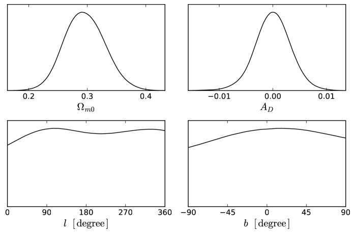
Figure 3: The marginalized probability distributions of $\Omega_{m0}$, the dipole magnitude $A_{D}$ and the dipole direction $(l,\,b)$, obtained by using the DF method to the JLA SNIa dataset without any prior on $\Omega_{m0}$ and $A_{D}$. See the text for details.

III Comparing two methods by using simulated SNIa datasets

As is shown in e.g. Chang:2014nca ; Yang:2013gea ; Lin:2015rza ; Chang:2017bbi and the previous section, the results from the HC method and the DF method are not always approximately coincident with each other. If these two methods find significantly different preferred directions, which one can be trusted? Both or none? If one method finds a preferred direction (or more) and the other method finds none, is the universe anisotropic or not? In this section, we try to shed new light on these questions. Our idea is to test these two methods by using several simulated anisotropic SNIa datasets with a preset preferred direction or more. We want to see which method can find out the preset direction(s), and whether the found direction(s) is/are close to the preset direction(s). In particular, we try to understand the results in Sec. II, namely why the DF method fails in the JLA SNIa dataset while the HC method works.

III.1 Methodology to generate the simulated SNIa datasets

For simplicity, and without loss of generality, we generate the simulated SNIa datasets like the Union2 or Union2.1 SNIa datasets, namely the simulated data tables are given directly in terms of the distance modulus $\mu$ (with $1\sigma$ uncertainty) versus the redshift $z$ of SNIa. Although the JLA/SNLS-like simulated SNIa datasets are more complicated mainly due to the extra parameters $\alpha$, $\beta$ in the distance estimate, the results obtained in this work can be easily extended to such kind of simulated datasets.

We take the future SNIa projects in the next decade as a reference to generate the simulated SNIa datasets. In this regard, the Wide Field Infrared Survey Telescope (WFIRST) Spergel:2015sza ; Spergel:2013uha ; WFIRSTwiki ; Hounsell:2017ejq to be launched in the mid-2020s might be a suitable reference. According to e.g. Hounsell:2017ejq , about $3000\sim 8000$ SNIa at $z\leq 1.7$ will be available from WFIRST. So, in the present work, we will generate $\sim 5000$ simulated SNIa in each dataset. Of course, the redshift distribution of SNIa tilts to the low-redshift range, and we can use a suitable F-distribution Fdis (say, $f(z,\,50,\,0.5)$) to mimic the one expected in e.g. Hounsell:2017ejq . According to e.g. Spergel:2013uha , the expected aggregate precision of these SNIa is $0.20\%$ at $z<1$ and $0.34\%$ at $z>1$. Therefore, we assign the simulated $1\sigma$ relative uncertainty of the distance modulus $\mu$ to be $0.20\%$ at $z<1$ and $0.35\%$ at $z\geq 1$ reasonably.

We generate the distance modulus $\mu$ of the simulated SNIa by taking a random number from a Gaussian distribution with the mean determined by a flat $\Lambda$CDM model,

$$\displaystyle\mu_{\rm mean}=5\log_{10}\frac{d_{L}}{\rm Mpc}+25\,,\hskip 56.9055ptd_{L}=\frac{c\left(1+z\right)}{H_{0}}\int_{0}^{z}\frac{d\tilde{z}}{E(\tilde{z})}\,,$$

$$E(z)=\left[\,\Omega_{m0}(1+z)^{3}+\left(1-\Omega_{m0}\right)\,\right]^{1/2}\,,$$ (13)

where $c$ is the speed of light, and the value of $\Omega_{m0}$ will be specified in the particular generating description. The Hubble constant $H_{0}=70\,{\rm km/s/Mpc}$ is adopted as a fiducial value, but it does not significantly affect other parameters since $H_{0}$ will be marginalized in fact. The standard deviation of this Gaussian distribution is equal to the $1\sigma$ uncertainty of $\mu$ mentioned above for the particular SNIa, namely $0.20\%$ of $\mu_{\rm mean}$ at $z<1$ and $0.35\%$ of $\mu_{\rm mean}$ at $z\geq 1$.

Finally, the galactic coordinates $(l,\,b)$ of the simulated SNIa will be specified in the particular generating description (see below). In fact, the position of the simulated SNIa and the value of $\Omega_{m0}$ mentioned above will play an important role.

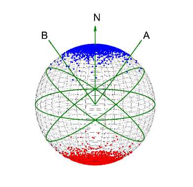
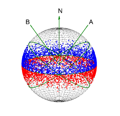
Figure 4: Demonstration of the spatial distributions of the “Pole-centralized” (left panel) and “Equator-centralized” (right panel) simulated SNIa, before they are rotated to a preset direction. The blue and red points are the SNIa generated with a relatively large and small $\Omega_{m0}$, respectively. See the text for details.

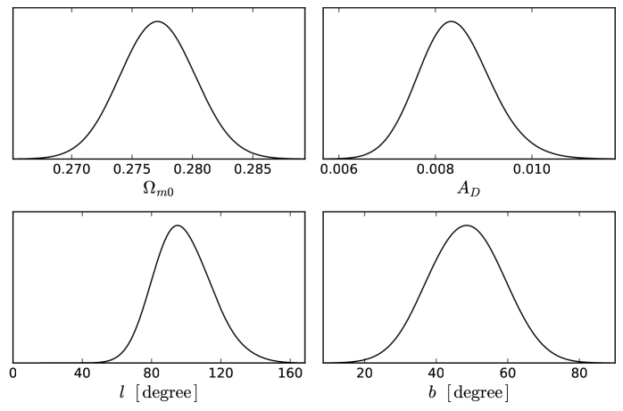
Figure 5: The marginalized probability distributions of $\Omega_{m0}$, the dipole magnitude $A_{D}$ and the dipole direction $(l,\,b)$, obtained by using the DF method to the simulated SNIa dataset PC1. See the text for details.

III.2 The cases of “Pole-centralized” simulated SNIa datasets

Let us generate the first simulated SNIa dataset. Here, we briefly describe the main steps:

1. Construct a Gaussian distribution with the mean at the north pole, and a suitable standard deviation (say, $30^{\circ}$). Assign a random number taken from this Gaussian distribution to a simulated SNIa as its galactic latitude $b$, and assign a random number uniformly taken from $[\,0^{\circ},\,360^{\circ})$ to this simulated SNIa as its galactic longitude $l$.

2. Assign a random redshift from a suitable F-distribution (say, $f(z,\,50,\,0.5)$) to this simulated SNIa as described in Sec. III.1.

3. Generate a distance modulus $\mu$ with $1\sigma$ uncertainty for this simulated SNIa by using a flat $\Lambda$CDM model with a relatively large $\Omega_{m0}$ (say, $0.45$), as described in Sec. III.1.

4. Repeat steps (P1$\sim$3) for 2500 times to generate 2500 simulated SNIa in the north hemisphere.

5. Generate 2500 simulated SNIa in the south hemisphere with a relatively small $\Omega_{m0}$ (say, $0.15$), similar to the previous steps.

6. By using a suitable coordinate transformation, rotate the whole celestial sphere (and all the 5000 simulated SNIa adhered to it) to any preset direction (say, $(l,\,b)=(120^{\circ},\,45^{\circ})$).

When steps (P1$\sim$5) are finished, the sky looks like the left panel of Fig. 4. Clearly, most of the simulated SNIa centralize around the north and south poles. So, we say such kind of simulated SNIa dataset is “Pole-centralized”. The degree of centralization is controlled by the specified standard deviation in step (P1). We call the simulated SNIa dataset with the specified parameters in the above steps as “PC1”.

We implement the HC method to the simulated SNIa dataset PC1, and repeat 15000 random directions $(l,\,b)$ across the whole sky. We find the $1\sigma$ angular region with the maximum AL is in the direction

$$(l,\,b)\,_{\rm HC}^{\rm PC1}=({138.4632^{\circ}}\,^{+25.0076^{\circ}}_{-49.2667^{\circ}}\,,\,{48.5212^{\circ}}\,^{+19.7711^{\circ}}_{-25.9446^{\circ}})\,,$$ (14)

and the corresponding maximum AL (with $1\sigma$ uncertainty) is

$${\rm AL_{max}^{PC1}}=1.0150\pm 0.0080\,.$$ (15)

Obviously, the direction given in Eq. (14) found by the HC method is approximately coincident with the preset direction $(120^{\circ},\,45^{\circ})$, but the $1\sigma$ uncertainties are fairly large.

Next, we consider the DF method. Noting that $A_{D}\left(\hat{n}\cdot\hat{p}\right)=-A_{D}\left(-\hat{n}\cdot\hat{p}\right)$ in Eq. (7), a positive $A_{D}$ with a direction $\hat{n}$ is equivalent to a negative $A_{D}$ with an opposite direction $-\hat{n}$. Actually, we have already implemented the DF method for many times in various cases, and indeed found two peaks in the results, but they are equivalent to each other in fact. Therefore, in the rest of this work, without loss of generality, we require $A_{D}\geq 0$ following e.g. Lin:2015rza .

We implement the DF method with the prior $A_{D}\geq 0$ to the simulated SNIa dataset PC1, and show the marginalized probability distributions of $\Omega_{m0}$, the dipole magnitude $A_{D}$ and the dipole direction $(l,\,b)$ in Fig. 5. The constraints with $1\sigma$ uncertainties are given by

$$\Omega_{m0}=0.2771^{+0.0031}_{-0.0031}\,,~{}~{}~{}~{}~{}~{}~{}~{}~{}~{}A_{D}=(8.4164^{+0.6831}_{-0.8011})\times 10^{-3}\,,$$ (16)

$$(l,\,b)\,_{\rm DF}^{\rm PC1}=({98.4333^{\circ}}\,^{+14.6610^{\circ}}_{-18.3059^{\circ}}\,,\,{48.4438^{\circ}}\,^{+10.5712^{\circ}}_{-10.5792^{\circ}})\,.$$ (17)

Although the $1\sigma$ uncertainties are relatively small, the direction given in Eq. (17) found by the DF method deviates from the preset direction $(120^{\circ},\,45^{\circ})$ beyond $1\sigma$ (notice that $l=120^{\circ}$ is out of the $1\sigma$ region given in Eq. (17)). Nonetheless, it is still close to the preset direction within the $2\sigma$ region.

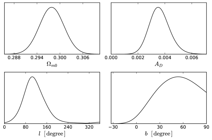
Figure 6: The same as in Fig. 5, except for the simulated SNIa dataset PC2. See the text for details.

Noting that in the simulated SNIa dataset PC1, the preset ${\rm AL}\sim 2\,(0.45-0.15)/(0.45+0.15)=1$ is fairly high, it is natural to see what will happen in the case of lower preset AL. So, we generate the second “Pole-centralized” simulated SNIa dataset PC2, by replacing the values of $\Omega_{m0}$ in steps (P3) and (P5) with $0.36$ and $0.24$, respectively. In this case, the preset ${\rm AL}\sim 2\,(0.36-0.24)/(0.36+0.24)=0.4$.

We implement the HC method to the simulated SNIa dataset PC2, and repeat 15000 random directions $(l,\,b)$ across the whole sky. We find the $1\sigma$ angular region with the maximum AL is in the direction

$$(l,\,b)\,_{\rm HC}^{\rm PC2}=({116.9953^{\circ}}\,^{+51.9794^{\circ}}_{-44.0647^{\circ}}\,,\,{44.7026^{\circ}}\,^{+34.6490^{\circ}}_{-23.2385^{\circ}})\,,$$ (18)

and the corresponding maximum AL (with $1\sigma$ uncertainty) is

$${\rm AL_{max}^{PC2}}=0.4057\pm 0.0076\,.$$ (19)

Again, the direction given in Eq. (18) found by the HC method is approximately coincident with the preset direction $(120^{\circ},\,45^{\circ})$, but the $1\sigma$ uncertainties are very large.

Then, we implement the DF method with the prior $A_{D}\geq 0$ to the simulated SNIa dataset PC2, and show the marginalized probability distributions of $\Omega_{m0}$, the dipole magnitude $A_{D}$ and the dipole direction $(l,\,b)$ in Fig. 6. The constraints with $1\sigma$ uncertainties are

$$\Omega_{m0}=0.2979^{+0.0031}_{-0.0032}\,,~{}~{}~{}~{}~{}~{}~{}~{}~{}~{}A_{D}=(3.6069^{+0.6765}_{-0.8190})\times 10^{-3}\,,$$ (20)

$$(l,\,b)\,_{\rm DF}^{\rm PC2}=({116.0269^{\circ}}\,^{+30.2393^{\circ}}_{-47.2547^{\circ}}\,,\,{49.3230^{\circ}}\,^{+30.5256^{\circ}}_{-20.4601^{\circ}})\,.$$ (21)

It is easy to see that the direction given in Eq. (21) found by the DF method is approximately coincident with the preset direction $(120^{\circ},\,45^{\circ})$, but the $1\sigma$ uncertainties are also very large.

The common feature in the “Pole-centralized” simulated SNIa datasets is that the uncertainties of the preferred direction are fairly large. One can understand this from the left panel of Fig. 4. Since the simulated SNIa centralize around two poles, the SNIa located in the “up hemisphere” and the “down hemisphere” are almost the same for e.g. the directions A, B and N in the left panel of Fig. 4, although these directions are far from each other. Therefore, the values of AL for the directions A, B and N are fairly close. As a natural consequence, the preferred directions found by both the HC and the DF methods can deviate from the preset direction, and the $1\sigma$ angular region must be fairly large. Of course, the preset direction is still within the $1\sigma$ ($2\sigma$) angular region found by the HC (DF) method, while the results of these two methods are consistent with each other at the $1\sigma$ level.

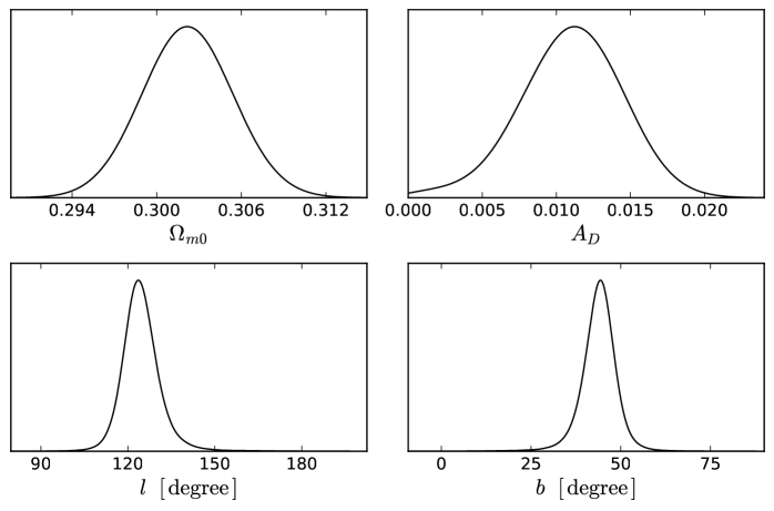
Figure 7: The same as in Fig. 5, except for the simulated SNIa dataset EC1. See the text for details.

III.3 The cases of “Equator-centralized” simulated SNIa datasets

As is discussed above, the uncertainties of the preferred direction in the “Pole-centralized” simulated SNIa datasets are commonly large. So, we consider another kind of simulated SNIa datasets, which are generated in a significantly different way. The main steps are

1. Construct a Gaussian distribution with the mean at the equator (i.e. $b=0$), and a suitable standard deviation (say, $10^{\circ}$). Assign a random number taken from this Gaussian distribution to a simulated SNIa as its galactic latitude $b$, and assign a random number uniformly taken from $[\,0^{\circ},\,360^{\circ})$ to this simulated SNIa as its galactic longitude $l$.

2. Assign a random redshift from a suitable F-distribution (say, $f(z,\,50,\,0.5)$) to this simulated SNIa as described in Sec. III.1.

3. Generate a distance modulus $\mu$ with $1\sigma$ uncertainty for this simulated SNIa by using a flat $\Lambda$CDM model with a relatively large $\Omega_{m0}$ (say, $0.36$) if its galactic latitude $b\geq 0$, or with a relatively small $\Omega_{m0}$ (say, $0.24$) if its galactic latitude $b<0$, as described in Sec. III.1.

4. Repeat steps (E1$\sim$3) for 5000 times to generate 5000 simulated SNIa in the whole celestial sphere. Notice that the galactic latitudes $b>,\,=,\,<0$ correspond to the north hemisphere, the equator, the south hemisphere, respectively.

5. By using a suitable coordinate transformation, rotate the whole celestial sphere (and all the 5000 simulated SNIa adhered to it) to any preset direction (say, $(l,\,b)=(120^{\circ},\,45^{\circ})$).

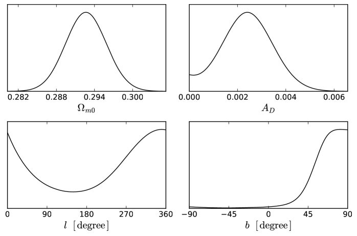
Figure 8: The same as in Fig. 5, except for the simulated SNIa dataset EC2_d. See the text for details.

When steps (E1$\sim$4) are finished, the sky looks like the right panel of Fig. 4. Clearly, most of the simulated SNIa centralize around the equator. Thus, we say such kind of simulated SNIa dataset is “Equator-centralized”. The degree of centralization is controlled by the specified standard deviation in step (E1). We call the simulated SNIa dataset with the specified parameters in the above steps as “EC1”.

In contrast to the “Pole-centralized” simulated SNIa dataset, since the “Equator-centralized” simulated SNIa centralize around the equator, the SNIa located in the “up hemisphere” and the “down hemisphere” for e.g. the directions A and B in the right panel of Fig. 4 are significantly different from the ones for the direction N. Noting that the blue and red points have different $\Omega_{m0}$, it is easy to imagine that the directions significantly deviating from the direction N will have a much lower AL than the one of the direction N. As a natural consequence, the preferred direction found by both the HC and the DF methods cannot significantly deviate from the preset direction, and the $1\sigma$ angular region must be very small.

We implement the HC method to the simulated SNIa dataset EC1, and first repeat 15000 random directions $(l,\,b)$ across the whole sky. We find that the directions with the largest ALs concentrate around $(121.4857^{\circ},\,44.7463^{\circ})$, but the test random directions within the $1\sigma$ region are fairly few. As is discussed above, this is not surprising due to the very small $1\sigma$ angular region expected in the cases of “Equator-centralized” simulated SNIa datasets. Similar to the case of JLA SNIa dataset, we densely repeat 5000 random directions from a Gaussian distribution with the mean in this preliminary direction. Finally, we find the $1\sigma$ angular region with the maximum AL is in the direction

$$(l,\,b)\,_{\rm HC}^{\rm EC1}=({120.2120^{\circ}}\,^{+0.5732^{\circ}}_{-1.2585^{\circ}}\,,\,{44.8209^{\circ}}\,^{+0.9175^{\circ}}_{-0.2926^{\circ}})\,,$$ (22)

and the corresponding maximum AL (with $1\sigma$ uncertainty) is

$${\rm AL_{max}^{EC1}}=0.4138\pm 0.0076\,.$$ (23)

Obviously, the direction given in Eq. (22) found by the HC method is excellently coincident with the preset direction $(120^{\circ},\,45^{\circ})$, and the $1\sigma$ uncertainties are very small, as expected above.

We implement the DF method with the prior $A_{D}\geq 0$ to the simulated SNIa dataset EC1, and show the marginalized probability distributions of $\Omega_{m0}$, the dipole magnitude $A_{D}$ and the dipole direction $(l,\,b)$ in Fig. 7. The constraints with $1\sigma$ uncertainties are given by

$$\Omega_{m0}=0.3022^{+0.0032}_{-0.0032}\,,~{}~{}~{}~{}~{}~{}~{}~{}~{}~{}A_{D}=(1.0991^{+0.3668}_{-0.3250})\times 10^{-2}\,,$$ (24)

$$(l,\,b)\,_{\rm DF}^{\rm EC1}=({124.7959^{\circ}}\,^{+5.0194^{\circ}}_{-6.7571^{\circ}}\,,\,{43.8235^{\circ}}\,^{+4.6989^{\circ}}_{-3.9193^{\circ}})\,.$$ (25)

Again, the direction given in Eq. (25) found by the DF method is approximately coincident with the preset direction $(120^{\circ},\,45^{\circ})$, and the $1\sigma$ uncertainties are fairly small, as expected above.

It is easy to see that both the HC and the DF methods work very well in the cases of “Equator-centralized” simulated SNIa datasets. They can find the preset direction correctly, and their results are consistent with each other at the $1\sigma$ level.

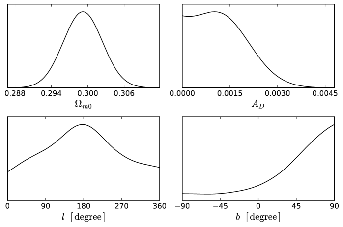
Figure 9: The same as in Fig. 5, except for the simulated SNIa dataset EC3_d. See the text for details.

III.4 The cases of simulated SNIa datasets with double preset directions

It is suggestive to ponder on the JLA SNIa dataset, where the HC method works but the DF method fails. The most noticeable feature of the JLA SNIa dataset is that there are two (or even more) preferred directions, as is shown in Sec. II. Therefore, we turn to consider the simulated SNIa datasets with double preset directions, which can be easily generated by combining two simulated SNIa datasets with different preset directions.

As is discussed in Sec. III.3, the $1\sigma$ uncertainties of the preferred direction are fairly small in the case of the “Equator-centralized” simulated SNIa datasets. So, we choose to combine two “Equator-centralized” simulated SNIa datasets, namely 2500 simulated SNIa with the preset direction $(300^{\circ},\,45^{\circ})$ and another 2500 simulated SNIa with the preset direction $(30^{\circ},\,0^{\circ})$. Note that the relevant parameters take the same values specified in steps (E1$\sim$3). We call the resulting simulated SNIa dataset “EC2_d”, which consists of 5000 simulated SNIa.

We implement the HC method to the simulated SNIa dataset EC2_d, and first repeat 15000 random directions $(l,\,b)$ across the whole sky. We find that the directions with the largest ALs concentrate around two directions, i.e. $(298.9182^{\circ},\,45.2628^{\circ})$ and $(30.2720^{\circ},\,0.2312^{\circ})$. Again, we densely repeat $5000+5000$ random directions from the Gaussian distributions with the means in these two preliminary directions, respectively. Finally, we find the $1\sigma$ angular region with the maximum AL is in the direction

$$(l,\,b)\,_{\rm HC,\,max}^{{\rm EC2}_{d}}=({29.8852^{\circ}}\,^{+0.4980^{\circ}}_{-0.3569^{\circ}}\,,\,{-0.1492^{\circ}}\,^{+0.3091^{\circ}}_{-0.2171^{\circ}})\,,$$ (26)

and the corresponding maximum AL (with $1\sigma$ uncertainty) is

$${\rm AL}_{\rm max}^{{\rm EC2}_{d}}=0.2206\pm 0.0078\,.$$ (27)

In addition, we also find a sub-maximum AL in the direction (with $1\sigma$ uncertainty)

$$(l,\,b)\,_{\rm HC,\,sub}^{{\rm EC2}_{d}}=({299.9246^{\circ}}\,^{+1.0814^{\circ}}_{-1.4783^{\circ}}\,,\,{44.5268^{\circ}}\,^{+0.7310^{\circ}}_{-1.3538^{\circ}})\,,$$ (28)

and the corresponding sub-maximum AL (with $1\sigma$ uncertainty) is

$${\rm AL}_{\rm sub}^{{\rm EC2}_{d}}=0.1538\pm 0.0077\,.$$ (29)

Clearly, these two preferred directions given in Eqs. (26) and (28) found by the HC method are excellently coincident with the two preset directions $(30^{\circ},\,0^{\circ})$ and $(300^{\circ},\,45^{\circ})$, while the $1\sigma$ uncertainties are very small, as expected above. The HC method works very well.

We implement the DF method with the prior $A_{D}\geq 0$ to the simulated SNIa dataset EC2_d, and show the marginalized probability distributions of $\Omega_{m0}$, the dipole magnitude $A_{D}$ and the dipole direction $(l,\,b)$ in Fig. 8. The constraints with $1\sigma$ uncertainties are given by

$$\Omega_{m0}=0.2927^{+0.0032}_{-0.0032}\,,~{}~{}~{}~{}~{}~{}~{}~{}~{}~{}A_{D}=(2.3638^{+1.0354}_{-1.0541})\times 10^{-3}\,,$$ (30)

$$(l,\,b)\,_{\rm DF}^{{\rm EC2}_{d}}=({183.4706^{\circ}}\,^{+176.5294^{\circ}}_{-183.4706^{\circ}}\,,\,{64.1008^{\circ}}\,^{+25.8992^{\circ}}_{-4.1372^{\circ}})\,.$$ (31)

Obviously, the DF method cannot correctly find out any one of the two preset directions $(300^{\circ},\,45^{\circ})$ and $(30^{\circ},\,0^{\circ})$, while the $1\sigma$ uncertainties are very large. In fact, the $1\sigma$ regions of $l$ and $b$ are $0^{\circ}\leq l\leq 360^{\circ}$ and $59.9636^{\circ}\leq b\leq 90^{\circ}$, respectively. That is, it “finds” a very wide $1\sigma$ angular region, which is not true in fact. The DF method fails in this case.

Further, we consider a fairly different case, in which the simulated SNIa are more centralized around the equator. We generate another simulated SNIa dataset EC3_d, which is the same as EC2_d but the specified standard deviation in step (E1) is replaced with $2^{\circ}$.

We implement the HC method to the simulated SNIa dataset EC3_d, and first repeat 15000 random directions $(l,\,b)$ across the whole sky. We find that the directions with the largest ALs concentrate around two directions, i.e. $(299.5397^{\circ},\,45.6902^{\circ})$ and $(30.7204^{\circ},\,-0.5147^{\circ})$. Again, we densely repeat $5000+5000$ random directions from the Gaussian distributions with the means in these two preliminary directions, respectively. Finally, we find the $1\sigma$ angular region with the maximum AL is in the direction

$$(l,\,b)\,_{\rm HC,\,max}^{{\rm EC3}_{d}}=({30.1148^{\circ}}\,^{+0.1339^{\circ}}_{-0.3388^{\circ}}\,,\,{-0.1085^{\circ}}\,^{+0.1916^{\circ}}_{-0.2465^{\circ}})\,,$$ (32)

and the corresponding maximum AL (with $1\sigma$ uncertainty) is

$${\rm AL}_{\rm max}^{{\rm EC3}_{d}}=0.2058\pm 0.0076\,.$$ (33)

In addition, we also find a sub-maximum AL in the direction (with $1\sigma$ uncertainty)

$$(l,\,b)\,_{\rm HC,\,sub}^{{\rm EC3}_{d}}=({299.9898^{\circ}}\,^{+0.2998^{\circ}}_{-0.1614^{\circ}}\,,\,{44.9113^{\circ}}\,^{+0.3212^{\circ}}_{-0.0486^{\circ}})\,,$$ (34)

and the corresponding sub-maximum AL (with $1\sigma$ uncertainty) is

$${\rm AL}_{\rm sub}^{{\rm EC3}_{d}}=0.1738\pm 0.0076\,.$$ (35)

In this case, these two preferred directions given in Eqs. (32) and (34) found by the HC method are still excellently coincident with the two preset directions $(30^{\circ},\,0^{\circ})$ and $(300^{\circ},\,45^{\circ})$, while the $1\sigma$ uncertainties are very small. The HC method still works very well.

We implement the DF method with the prior $A_{D}\geq 0$ to the simulated SNIa dataset EC3_d, and show the marginalized probability distributions of $\Omega_{m0}$, the dipole magnitude $A_{D}$ and the dipole direction $(l,\,b)$ in Fig. 9. The constraints with $1\sigma$ uncertainties are given by

$$\Omega_{m0}=0.2992^{+0.0032}_{-0.0032}\,,~{}~{}~{}~{}~{}~{}~{}~{}~{}~{}A_{D}=(1.2781^{+0.3608}_{-1.2707})\times 10^{-3}\,,$$ (36)

$$(l,\,b)\,_{\rm DF}^{{\rm EC3}_{d}}=({181.1659^{\circ}}\,^{+100.9199^{\circ}}_{-100.0070^{\circ}}\,,\,{42.6214^{\circ}}\,^{+47.3786^{\circ}}_{-7.9784^{\circ}})\,.$$ (37)

Again, the DF method cannot correctly find out any one of the two preset directions $(300^{\circ},\,45^{\circ})$ and $(30^{\circ},\,0^{\circ})$, while the $1\sigma$ uncertainties are very large. In fact, the $1\sigma$ regions of $l$ and $b$ are $81.1589^{\circ}\leq l\leq 282.0858^{\circ}$ and $34.6430^{\circ}\leq b\leq 90^{\circ}$, respectively. That is, it “finds” a very wide but wrong $1\sigma$ angular region. The DF method fails once more.

Clearly, the DF method cannot find any preset directions in the above two cases. Thus, we conclude that the DF method cannot properly work in the SNIa datasets with two (or even more) preferred directions, while the HC method still works well. In particular, this might help us to understand the results in the JLA SNIa dataset (see Sec. II). Briefly, as is found in Sec. II, there exist at least two preferred directions $(23.49^{\circ},\,2.25^{\circ})$ and $(299.47^{\circ},\,28.39^{\circ})$ in the JLA SNIa dataset, and hence it is not surprising that the DF method fails in this case. The JLA SNIa dataset is indeed a realistic example to show the shortcoming of the DF method.

Dataset	Preferred direction $(l,\,b)$	Ref.
Union2 SNIa (HC)	$(309^{\circ},\,18^{\circ})$	Antoniou:2010gw
Union2 SNIa (DF)	$(309^{\circ},\,-15^{\circ})$	Mariano:2012wx
Union2.1 SNIa (DF)	$(307^{\circ},\,-14^{\circ})$	Yang:2013gea
CMB Dipole	$(264^{\circ},\,48^{\circ})$	Lineweaver:1996xa
Velocity Flows	$(282^{\circ},\,6^{\circ})$	Feldman:2009es
Quasar Alignment	$(267^{\circ},\,69^{\circ})$	Hutsemekers
GRBs + Union2.1 SNIa (DF)	$(309^{\circ},\,-8.6^{\circ})$	Wang:2014vqa
$\Delta\alpha/\alpha$	$(330^{\circ},\,-13^{\circ})$	King:2012id ; Webb:2010hc
CMB Quadrupole	$(240^{\circ},\,63^{\circ})$	Frommert:2009qw ; Bielewicz:2004en
CMB Octopole	$(308^{\circ},\,63^{\circ})$	Bielewicz:2004en
SPARC Galaxies (HC max.)	$(175.5^{\circ},\,-6.5^{\circ})$	Zhou:2017lwy
SPARC Galaxies (HC sub-max.)	$(114.5^{\circ},\,2.5^{\circ})$	Zhou:2017lwy
SPARC Galaxies (DF)	$(171^{\circ},\,-15^{\circ})$	Chang:2018vxs
JLA SNIa (HC max.)	$(23.49^{\circ},\,2.25^{\circ})$	This work
JLA SNIa (HC sub-max.)	$(299.47^{\circ},\,28.39^{\circ})$	This work

Table 1: Preferred directions $(l,\,b)$ found in various observational datasets.

IV Concluding remarks

The cosmological principle is one of the cornerstones in modern cosmology Weinberg:cos ; Kolb90 . It assumes that the universe is homogeneous and isotropic on cosmic scales. Both the homogeneity and the isotropy of the universe should be tested carefully. In the present work, we are interested in probing the possible preferred direction in the distribution of SNIa. To our best knowledge, two main methods have been used in almost all of the relevant works in the literature, namely the HC method and the DF method. However, the results from these two methods are not always approximately coincident with each other. In this work, we test the cosmic anisotropy by using these two methods with the JLA and simulated SNIa datasets. In many cases, both methods work well, and their results are consistent with each other. However, in the cases with two (or even more) preferred directions, the DF method fails while the HC method still works well. This might shed new light on our understanding of these two methods.

In Table 1, we summarize the preferred directions $(l,\,b)$ found in various observational datasets. We also plot them in Fig. 10. Most of them (including the two preferred directions of the JLA SNIa dataset found in this work) are located in a relatively small part (about a quarter) of the north galactic hemisphere, as is shown by the red points in Fig. 10. In some sense, they are in agreement with each other. However, the three preferred directions found in the SPARC Galaxies are significantly different from the others, as is shown by the green points in Fig. 10. Note that these preferred directions in the SPARC Galaxies are found by using the centripetal acceleration $g_{\dagger}$ Zhou:2017lwy ; Chang:2018vxs . This is different from the others, and might be responsible for the difference. Nevertheless, we stress that the two preferred directions of the JLA SNIa dataset found in this work are clearly in agreement with the other ten preferred directions.

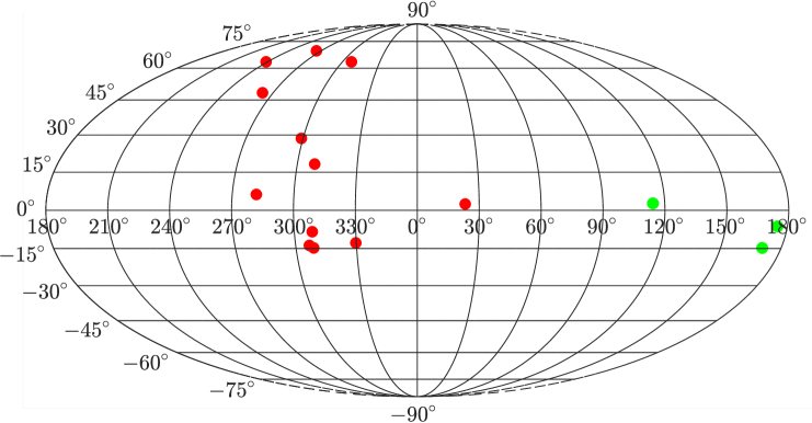
Figure 10: Preferred directions $(l,\,b)$ found in various observational datasets (see Table 1). Note that the three preferred directions in the SPARC Galaxies are labeled by the green points, while the others are labeled by the red points. See the text and Table 1 for details.

Several remarks are in order. In this work, we only consider the spatially flat $\Lambda$CDM model. In fact, one can generalize our discussions to other cosmological models, such as $w$CDM, CPL models. Of course, one can also consider model-independent parameterizations. It is reasonable to expect that our results do not change significantly in these generalized cases.

In the HC method, we have used $\Omega_{m0}$ (equivalent to the accelerating expansion rate, namely the deceleration parameter $q_{0}$, in the spatially flat $\Lambda$CDM model) to define AL, as in Eq. (1). In fact, one can instead define AL by using other quantities characterizing the cosmic expansion, e.g. the deceleration parameter $q_{0}$ directly Cai:2011xs and the Hubble rate $H_{0}$ Chang:2014nca .

Here, we have only considered the SNIa datasets. In fact, one can extend our work to the data of other observations, such as GRBs Meszaros:2009ux ; Wang:2014vqa ; Chang:2014jza ; Liu:2014vda , rotationally supported galaxies Zhou:2017lwy ; Chang:2018vxs , quasars and radio galaxies Singal:2013aga , quasar optical polarization data Hutsemekers ; Pelgrims:2016mhx , and the varying fine structure “constant” $\alpha$ Mariano:2012wx .

In this work, we have only considered two kinds of simulated SNIa datasets, which are “Pole-centralized” and “Equator-centralized”, respectively. In fact, one can further consider other kinds of simulated SNIa datasets. The distribution of simulated SNIa can be more general. On the other hand, one can further consider the simulated SNIa datasets with three or four preset directions to test both the HC method and the DF method.

Here are further discussions on the failure of the DF method in the cases with two (or even more) preferred directions. Since the DF method only models a single dipole, this failure is not surprising in fact. It is of interest to test the DF method and the HC method by using the simulated SNIa datasets with multiple dipoles of different amplitudes (we thank the anonymous referee A for pointing out this issue). However, we admit that it is fairly difficult to generate such kind of simulated SNIa datasets, and some smart ideas are needed to this end. We leave it to future work. On the other hand, the DF method might be improved by adding a quadrupole term in Eq. (7), or by simply generalizing the angular dependent function, e.g. replacing $\hat{n}\cdot\hat{p}$ with a function of $\hat{n}\cdot\hat{p}$ (we thank the anonymous referee B for pointing out this issue). In addition, although the monopole term does not encode the information of anisotropy and is indeed negligible in most of the relevant works, it is still of interest to identify the corresponding effect in the context of the DF method (we thank again the anonymous referee B for pointing out this issue). Since both improvements will remarkably extend the length of this paper, we hope to consider these issues in future work.

Although we have shown that the HC method works well while the DF method might fail in some complicated cases, it does not mean that one should not continue to use the DF method in the relevant works. Actually, the DF method works well in most cases and the corresponding results are approximately coincident with the ones of the HC method. Most importantly, the DF method is more efficient than the HC method, namely it consumes less computational power and time. In the HC method, in order to find the preferred direction precisely, one needs to significantly increase the number of the random directions in searching the direction with the maximum AL. For example, it took more than 1 week to calculate the ALs for $\sim 40000$ random directions in the JLA SNIa dataset (see Sec. II) by using our computer. However, employing the MCMC code CosmoMC Lewis:2002ah instead, the DF method only took $\sim 10$ hours to obtain the satisfactory result by using the same computer. The algorithm of the DF method makes it more efficient than the HC method, and hence the DF method is still a valuable tool in the relevant works.

Since they have been used extensively in the literature, we consider that both the HC method and the DF method need to be improved. Further corrections or even completely new methods are desirable. New ideas are welcome.

References

-
(1)
S. Weinberg, Gravitation and Cosmology,
John Wiley & Sons, Inc., New York (1972);
S. Weinberg, Cosmology, Oxford University Press, Oxford (2008). - (2) E. W. Kolb and M. S. Turner, The Early Universe, Addison Wesley (1990).
- (3) D. W. Hogg et al., Astrophys. J. 624, 54 (2005) [astro-ph/0411197].
-
(4)
A. Hajian and T. Souradeep,
Phys. Rev. D 74, 123521 (2006)
[astro-ph/0607153];
T. R. Jaffe et al., Astrophys. J. 629, L1 (2005) [astro-ph/0503213]. - (5) R. R. Caldwell and A. Stebbins, Phys. Rev. Lett. 100, 191302 (2008) [arXiv:0711.3459].
- (6) I. Zehavi, A. G. Riess, R. P. Kirshner and A. Dekel, Astrophys. J. 503, 483 (1998) [astro-ph/9802252].
- (7) A. G. Riess et al., Astron. J. 116, 1009 (1998) [astro-ph/9805201].
- (8) S. Perlmutter et al., Astrophys. J. 517, 565 (1999) [astro-ph/9812133].
-
(9)
E. J. Copeland, M. Sami and S. Tsujikawa,
Int. J. Mod. Phys. D 15, 1753 (2006) [hep-th/0603057];
A. Albrecht et al., astro-ph/0609591;
J. Frieman, M. Turner and D. Huterer, Ann. Rev. Astron. Astrophys. 46, 385 (2008) [arXiv:0803.0982];
S. Tsujikawa, arXiv:1004.1493 [astro-ph.CO];
M. Li et al., Commun. Theor. Phys. 56, 525 (2011) [arXiv:1103.5870];
L. Amendola et al., Living Rev. Rel. 16, 6 (2013) [arXiv:1206.1225]. -
(10)
A. De Felice and S. Tsujikawa,
Living Rev. Rel. 13, 3 (2010) [arXiv:1002.4928];
T. P. Sotiriou and V. Faraoni, Rev. Mod. Phys. 82, 451 (2010) [arXiv:0805.1726];
T. Clifton, P. G. Ferreira, A. Padilla and C. Skordis, Phys. Rept. 513, 1 (2012) [arXiv:1106.2476];
S. Nojiri and S. D. Odintsov, Phys. Rept. 505, 59 (2011) [arXiv:1011.0544];
Y. F. Cai et al., Rept. Prog. Phys. 79, 106901 (2016) [arXiv:1511.07586];
S. Nojiri, S. D. Odintsov and V. K. Oikonomou, Phys. Rept. 692, 1 (2017) [arXiv:1705.11098]. -
(11)
G. Lemaître,
Annales de la Société Scientifique de Bruxelles
A 53, 51 (1933),
see Gen. Rel. Grav. 29, 641 (1997) for English translation;
R. C. Tolman, Proc. Nat. Acad. Sci. 20, 169 (1934), see Gen. Rel. Grav. 29, 935 (1997) for English translation;
H. Bondi, Mon. Not. Roy. Astron. Soc. 107, 410 (1947). - (12) S. W. Goode and J. Wainwright, Phys. Rev. D 26, 3315 (1982).
- (13) H. Alnes, M. Amarzguioui and O. Gron, Phys. Rev. D 73, 083519 (2006) [astro-ph/0512006].
- (14) J. Garcia-Bellido and T. Haugboelle, JCAP 0804, 003 (2008) [arXiv:0802.1523].
-
(15)
K. Enqvist and T. Mattsson,
JCAP 0702, 019 (2007)
[astro-ph/0609120];
K. Enqvist, Gen. Rel. Grav. 40, 451 (2008) [arXiv:0709.2044];
R. A. Vanderveld, E. E. Flanagan and I. Wasserman, Phys. Rev. D 74, 023506 (2006) [astro-ph/0602476];
J. P. Zibin, Phys. Rev. D 78, 043504 (2008) [arXiv:0804.1787];
M. N. Celerier, K. Bolejko and A. Krasinski, Astron. Astrophys. 518, A21 (2010) [arXiv:0906.0905];
M. N. Celerier, Astron. Astrophys. 543, A71 (2012) [arXiv:1108.1373]. - (16) M. N. Celerier, J. Phys. Conf. Ser. 484, 012005 (2014) [arXiv:1203.2814].
- (17) M. Ishak, A. Peel and M. A. Troxel, Phys. Rev. Lett. 111, no. 25, 251302 (2013) [arXiv:1307.0723].
- (18) T. Clifton, P. G. Ferreira and K. Land, Phys. Rev. Lett. 101, 131302 (2008) [arXiv:0807.1443].
-
(19)
Z. S. Zhang, T. J. Zhang, H. Wang and C. Ma,
Phys. Rev. D 91, 063506 (2015)
[arXiv:1210.1775];
H. Wang and T. J. Zhang, Astrophys. J. 748, 111 (2012) [arXiv:1111.2400]. - (20) X. P. Yan, D. Z. Liu and H. Wei, Phys. Lett. B 742, 149 (2015) [arXiv:1411.6218].
- (21) M. N. Celerier, Astron. Astrophys. 353, 63 (2000) [astro-ph/9907206].
- (22) J. W. Moffat, JCAP 0510, 012 (2005) [astro-ph/0502110].
- (23) H. Alnes and M. Amarzguioui, Phys. Rev. D 74, 103520 (2006) [astro-ph/0607334].
- (24) T. Clifton, P. G. Ferreira and J. Zuntz, JCAP 0907, 029 (2009) [arXiv:0902.1313].
- (25) C. Clarkson and M. Regis, JCAP 1102, 013 (2011) [arXiv:1007.3443].
- (26) A. Moss, J. P. Zibin and D. Scott, Phys. Rev. D 83, 103515 (2011) [arXiv:1007.3725].
- (27) J. P. Uzan, C. Clarkson and G. F. R. Ellis, Phys. Rev. Lett. 100, 191303 (2008) [arXiv:0801.0068].
- (28) M. Quartin and L. Amendola, Phys. Rev. D 81, 043522 (2010) [arXiv:0909.4954].
- (29) K. Bolejko and J. S. B. Wyithe, JCAP 0902, 020 (2009) [arXiv:0807.2891].
- (30) S. February, C. Clarkson and R. Maartens, JCAP 1303, 023 (2013) [arXiv:1206.1602].
- (31) J. P. Zibin, A. Moss and D. Scott, Phys. Rev. Lett. 101, 251303 (2008) [arXiv:0809.3761].
- (32) K. Tomita and K. T. Inoue, Phys. Rev. D 79, 103505 (2009) [arXiv:0903.1541].
- (33) F. S. Labini and Y. V. Baryshev, JCAP 1006, 021 (2010) [arXiv:1006.0801].
- (34) P. Zhang and A. Stebbins, Phys. Rev. Lett. 107, 041301 (2011) [arXiv:1009.3967].
- (35) W. Valkenburg et al., Mon. Not. Roy. Astron. Soc. 438, L6 (2014) [arXiv:1209.4078].
- (36) P. Bull, T. Clifton and P. G. Ferreira, Phys. Rev. D 85, 024002 (2012) [arXiv:1108.2222].
- (37) J. P. Zibin and A. Moss, Class. Quant. Grav. 28, 164005 (2011) [arXiv:1105.0909].
- (38) V. Marra and A. Notari, Class. Quant. Grav. 28, 164004 (2011) [arXiv:1102.1015].
- (39) K. Gödel, Rev. Mod. Phys. 21, 447 (1949).
-
(40)
S. L. Li, X. H. Feng, H. Wei and H. Lü,
Eur. Phys. J. C 77, no. 5, 289 (2017)
[arXiv:1612.02069];
W. J. Geng, S. L. Li, H. Lü and H. Wei, Phys. Lett. B 780, 196 (2018) [arXiv:1801.00009]. -
(41)
S. Kumar and C. P. Singh,
Astrophys. Space Sci. 312, 57 (2007);
R. Venkateswarlu and K. Sreenivas, Int. J. Theor. Phys. 53, 2051 (2014);
S. Ram and C. P. Singh, Astrophys. Space Sci. 257, 287 (1998);
L. Yadav, V. K. Yadav and T. Singh, Int. J. Theor. Phys. 51, 3113 (2012);
A. Pradhan and H. Amirhashchi, Astrophys. Space Sci. 332, 441 (2011) [arXiv:1010.2362];
D. K. Banik, S. K. Banik and K. Bhuyan, Astrophys. Space Sci. 362, 51 (2017);
B. Mishra, P. K. Sahoo and S. Suresh, Astrophys. Space Sci. 358, 7 (2015);
A. K. Yadav, Astrophys. Space Sci. 335, 565 (2011) [arXiv:1101.4349];
B. Saha, Int. J. Theor. Phys. 52, 3646 (2013) [arXiv:1209.6029];
J. M. Bradley and E. Sviestins, Gen. Rel. Grav. 16, 1119 (1984);
D. Lorenz, Phys. Rev. D 22, 1848 (1980);
D. Sofuoglu, Astrophys. Space Sci. 361, 12 (2016). -
(42)
K. Land and J. Magueijo,
Phys. Rev. Lett. 95, 071301 (2005)
[astro-ph/0502237];
K. Land and J. Magueijo, Mon. Not. Roy. Astron. Soc. 378, 153 (2007) [astro-ph/0611518];
K. Land and J. Magueijo, Mon. Not. Roy. Astron. Soc. 357, 994 (2005) [astro-ph/0405519]. - (43) W. Zhao and L. Santos, The Universe, no. 3, 9 (2015) [arXiv:1604.05484].
- (44) F. K. Hansen et al., Mon. Not. Roy. Astron. Soc. 354, 641 (2004) [astro-ph/0404206].
- (45) D. J. Schwarz and B. Weinhorst, Astron. Astrophys. 474, 717 (2007) [arXiv:0706.0165].
- (46) I. Antoniou and L. Perivolaropoulos, JCAP 1012, 012 (2010) [arXiv:1007.4347].
- (47) A. Mariano and L. Perivolaropoulos, Phys. Rev. D 86, 083517 (2012) [arXiv:1206.4055].
-
(48)
R. G. Cai and Z. L. Tuo,
JCAP 1202, 004 (2012)
[arXiv:1109.0941];
R. G. Cai, Y. Z. Ma, B. Tang and Z. L. Tuo, Phys. Rev. D 87, 123522 (2013) [arXiv:1303.0961]. - (49) W. Zhao, P. X. Wu and Y. Zhang, Int. J. Mod. Phys. D 22, 1350060 (2013) [arXiv:1305.2701].
- (50) X. Yang, F. Y. Wang and Z. Chu, Mon. Not. Roy. Astron. Soc. 437, 1840 (2014) [arXiv:1310.5211].
- (51) Z. Chang and H. N. Lin, Mon. Not. Roy. Astron. Soc. 446, 2952 (2015) [arXiv:1411.1466].
- (52) H. N. Lin, S. Wang, Z. Chang and X. Li, Mon. Not. Roy. Astron. Soc. 456, 1881 (2016) [arXiv:1504.03428].
- (53) Z. Chang, H. N. Lin, Y. Sang and S. Wang, arXiv:1711.11321 [astro-ph.CO].
- (54) A. Meszaros et al., AIP Conf. Proc. 1133, 483 (2009) [arXiv:0906.4034].
- (55) J. S. Wang and F. Y. Wang, Mon. Not. Roy. Astron. Soc. 443, no. 2, 1680 (2014) [arXiv:1406.6448].
- (56) Z. Chang, X. Li, H. N. Lin and S. Wang, Mod. Phys. Lett. A 29, 1450067 (2014) [arXiv:1405.3074].
- (57) Y. Zhou, Z. C. Zhao and Z. Chang, Astrophys. J. 847, no. 2, 86 (2017) [arXiv:1707.00417].
- (58) Z. Chang, H. N. Lin, Z. C. Zhao and Y. Zhou, arXiv:1803.08344 [astro-ph.CO].
- (59) A. K. Singal, Astrophys. Space Sci. 357, no. 2, 152 (2015) [arXiv:1305.4134].
-
(60)
D. Hutsemekers et al.,
Astron. Astrophys. 441, 915 (2005)
[astro-ph/0507274];
D. Hutsemekers and H. Lamy, Astron. Astrophys. 367, 381 (2001) [astro-ph/0012182];
D. Hutsemekers et al., ASP Conf. Ser. 449, 441 (2011) [arXiv:0809.3088] - (61) V. Pelgrims, arXiv:1604.05141 [astro-ph.CO].
- (62) J. K. Webb et al., Phys. Rev. Lett. 82, 884 (1999) [astro-ph/9803165].
-
(63)
J. K. Webb et al.,
Phys. Rev. Lett. 87, 091301 (2001)
[astro-ph/0012539];
M. T. Murphy et al., Mon. Not. Roy. Astron. Soc. 327, 1208 (2001) [astro-ph/0012419]. - (64) J. P. Uzan, Living Rev. Rel. 14, 2 (2011) [arXiv:1009.5514].
- (65) J. D. Barrow, Ann. Phys. 19, 202 (2010) [arXiv:0912.5510].
-
(66)
H. Wei,
Phys. Lett. B 682, 98 (2009)
[arXiv:0907.2749];
H. Wei, X. P. Ma and H. Y. Qi, Phys. Lett. B 703, 74 (2011) [arXiv:1106.0102];
H. Wei, X. B. Zou, H. Y. Li and D. Z. Xue, Eur. Phys. J. C 77, no. 1, 14 (2017) [arXiv:1605.04571];
H. Wei and D. Z. Xue, Commun. Theor. Phys. 68, no. 5, 632 (2017) [arXiv:1706.04063]. - (67) J. A. King et al., Mon. Not. Roy. Astron. Soc. 422, 3370 (2012) [arXiv:1202.4758].
- (68) J. K. Webb et al., Phys. Rev. Lett. 107, 191101 (2011) [arXiv:1008.3907].
-
(69)
M. Betoule et al.,
Astron. Astrophys. 568, A22 (2014)
[arXiv:1401.4064];
Since March 2014, the JLA plugin is included in the official release of CosmoMC;
http:supernovae.in2p3.fr/sdss-snls-jla/ReadMe.html -
(70)
X. B. Zou, H. K. Deng, Z. Y. Yin and H. Wei,
Phys. Lett. B 776, 284 (2018)
[arXiv:1707.06367];
H. Wei, Phys. Lett. B 692, 167 (2010) [arXiv:1005.1445];
H. Wei, X. B. Zou, H. Y. Li and D. Z. Xue, Eur. Phys. J. C 77, no. 1, 14 (2017) [arXiv:1605.04571];
H. Wei and D. Z. Xue, Commun. Theor. Phys. 68, no. 5, 632 (2017) [arXiv:1706.04063]. -
(71)
A. Lewis and S. Bridle,
Phys. Rev. D 66, 103511 (2002)
[astro-ph/0205436];
http:cosmologist.info/cosmomc/ -
(72)
D. Spergel et al.,
arXiv:1503.03757 [astro-ph.IM];
D. Spergel et al., arXiv:1305.5422 [astro-ph.IM];
J. Green et al., arXiv:1208.4012 [astro-ph.IM]. - (73) D. Spergel et al., arXiv:1305.5425 [astro-ph.IM].
- (74) https:en.wikipedia.org/wiki/Wide-Field-Infrared-Survey-Telescope
- (75) R. Hounsell et al., arXiv:1702.01747 [astro-ph.IM].
-
(76)
https:en.wikipedia.org/wiki/F-distribution
http:www.mathworks.com/help/stats/f-distribution.html -
(77)
J. Liu and H. Wei,
Gen. Rel. Grav. 47, no. 11, 141 (2015)
[arXiv:1410.3960];
H. Wei, JCAP 1008, 020 (2010) [arXiv:1004.4951]. - (78) C. H. Lineweaver et al., Astrophys. J. 470, 38 (1996) [astro-ph/9601151].
-
(79)
H. A. Feldman et al.,
Mon. Not. Roy. Astron. Soc. 407, 2328 (2010)
[arXiv:0911.5516];
R. Watkins et al., Mon. Not. Roy. Astron. Soc. 392, 743 (2009) [arXiv:0809.4041]. - (80) M. Frommert and T. A. Enßlin, Mon. Not. Roy. Astron. Soc. 403, 1739 (2010) [arXiv:0908.0453].
- (81) P. Bielewicz et al., Mon. Not. Roy. Astron. Soc. 355, 1283 (2004) [astro-ph/0405007].
-
(82)
B. Javanmardi et al.,
Astrophys. J. 810, no. 1, 47 (2015)
[arXiv:1507.07560];
H. N. Lin, X. Li and Z. Chang, Mon. Not. Roy. Astron. Soc. 460, no. 1, 617 (2016) [arXiv:1604.07505]. -
(83)
B. Mishra and S. K. Tripathy,
Mod. Phys. Lett. A 30, no. 36, 1550175 (2015)
[arXiv:1507.03515];
B. Mishra et al., Adv. High Energy Phys. 2018, 6306848 (2018) [arXiv:1706.07661];
B. Mishra, S. K. Tripathy and P. P. Ray, Astrophys. Space Sci. 363, 86 (2018) [arXiv:1701.08632]. -
(84)
C. A. P. Bengaly, A. Bernui and J. S. Alcaniz,
Astrophys. J. 808, 39 (2015)
[arXiv:1503.01413];
U. Andrade et al., Phys. Rev. D 97, no. 8, 083518 (2018) [arXiv:1711.10536]. - (85) C. A. P. Bengaly, R. Maartens and M. G. Santos, JCAP 1804, 031 (2018) [arXiv:1710.08804].