Localization transitions and mobility edges in coupled Aubry-André chains

Abstract

We study the localization transitions for coupled one-dimensional lattices with quasiperiodic potential. Besides the localized and extended phases there is an intermediate mixed phase which can be easily explained decoupling the system so as to deal with effective uncoupled Aubry-André chains with different transition points. We clarify, therefore, the origin of such an intermediate phase finding the conditions for getting a uniquely defined mobility edge for such coupled systems. Finally we consider many coupled chains with an energy shift which compose an extension of the Aubry-André model in two dimensions. We study the localization behavior in this case comparing the results with those obtained for a truly aperiodic two-dimensional (2D) Aubry-André model, with quasiperiodic potentials in any directions, and for the 2D Anderson model.

I Introduction

Since the discovery of the Anderson transition Anderson1958 , the problem of localization of the wavefunctions in low dimensional quantum systems has attracted a lot of both theoretical and experimental interest in the scientific community Mott ; Abrahams ; Harper ; Aubry ; Giamarchi ; Billy ; Roati . Anderson localization predicts that the single particle wavefunctions become localized in the presence of some uncorrelated disorder, leading to a metal-insulator transition caused by the quantum interference in the scattering processes of a particle with random impurities and defects.

Although the standard Anderson transition occurs in three dimensions, an analogous effect may appear in one dimension (1D) in the presence of a so-called quasi-disorder. The most popular case is provided by the well celebrated Aubry-André model Harper ; Aubry which exhibits a transition between a phase where all the eigenstates are localized and another one where they are extended. Generalizations of this model have been recently proposed by exponential short-range hopping Biddle , flatband networks flach2 , higher dimensions r1 , power-law hopping r2 , and breaking the time-reversal symmetry by a magnetic flux flux . Dynamical properties of a generalized Aubry-André model have also been investigated r3 .

Strongly motivated by the recent experiments of Bloch and cowokers Bordia ; Bordia2017 ; Luschen2017 and by the feasibility of realizing several copies of the Aubry-André system, by cold atoms or optical waveguides Kraus ; Lohse , we investigate the localization transitions for coupled-chains in a quasi-disordered environment. Moreover, in the experiment reported in Ref. Luschen2017 , a coexistence was observed of localized and delocalized states due to the extension of the kinetic term persisting even in the strong tight binding limit of a continuous one-dimensional bichromatic model, although, in that limit, there is not expected to be any range of parameters where localized and extended states can coexist. The authors in Ref. Luschen2017 explain the discrepancy between the theoretical predictions of a narrower intermediate phase and the observations by averaging over many Aubry-André chains produced in the experiment, which can have slightly different parameters, due to the finite extension of the beams creating the optical lattices, so that chains on the outside of the system can experience slightly lower lattice depths than those in the center. As we will see, an analogous effect can be obtained if one allows those chains to be coupled. In this case the intermediate phase of coexistence may increase and, eventually can contribute to the discrepancy discussed above.

We will perform, therefore, a systematic study of the localization transitions of two and many coupled chains in order to clarify also the appearance of the mobility edges in such composed systems. The presence of an intermediate phase where extended and localized states coexist make the definition of a mobility edge questionable Sil2008 ; Flach2014 . We make clear the origin of such an intermediate phase finding the conditions for a unique and well defined mobility edge for such aperiodic coupled chains. We will consider, finally, many coupled chains which have shifted energies one compared to the other, obtaining as a result a generalized Aubry-André model in two dimensions. We observe that in this case, on average, the extension of the wavefunctions, for large quasiperiodic potential is much larger than that obtained in the presence of a true uncorrelated disorder. A sharper localization is, instead, obtained by using quasiperiodic potentials in any directions, considering a truly aperiodic 2D Aubry-André model r1 .

The paper is organized as it follows: in Sec. II we will briefly review the known results for a single Aubry-André model, with both nearest-neighbor and further hopping terms, in Sec. III we will consider two coupled chains for short and longer hopping terms, discussing the intermediate phase, and in Sec. IV we will generalize the coupling to a generic number of chains. Finally, in Sec. V we will consider the generalization of the Aubry-André model in two dimensions, by coupling many chains or imposing aperiodic potentials in both directions, and make the comparison with the Anderson model.

II The Aubry-André model

Let us consider the following one-dimensional lattice model, called the Aubry-André chain,

$$\mathcal{H}=\sum_{i\neq j}t_{ij}{\hat{c}}^{\dagger}_{i}\hat{c}_{j}+\lambda\sum_{i}\cos(2\pi\tau i)\,{\hat{c}}^{\dagger}_{i}\hat{c}_{i}$$ (1)

where $\tau=\frac{1+\sqrt{5}}{2}$ is the golden ratio, ${\hat{c}_{i}}^{\dagger}$, $\hat{c}_{i}$ are the (bosonic or fermionic) creation and annihilation operators defined on the lattice site $i$, $t_{ij}$ the hopping parameter and $\lambda$ the strength of the quasi-disordered potential. It has been rigorously proven Jitomirskaya that if the sum is restricted to nearest-neighbor sites, $t_{ij}=t_{1}(\delta_{j,i+1}+\delta_{j,i-1})$, the above system shows a transition at

$$\lambda=\lambda_{c}=2t_{1}\,.$$ (2)

Above $\lambda_{c}$ all eigenstates are exponentially localized, while below they are all delocalized. On the other hand, if the sum is extended to further neighbors, there is a mobility edge Boers , namely, the critical strength of the potential $\lambda_{c}$, depends on the energy levels $E_{n}$, and providing that the hopping parameter decays exponentially with the distance ($|t_{\ell}|\equiv|t_{i,i\pm\ell}|=e^{-p\ell}$ with $p$ some positive real value), the transition can be calculated analytically Biddle ; Ramakumar2014

$$\lambda_{c}=\frac{2t_{1}+2E_{n}t_{2}/t_{1}}{1+(t_{2}/t_{1})^{2}}\,.$$ (3)

This expression is exact for exponential form of the hopping parameter but is also in a very good agreement with numerical results if one considers terms up to next-nearest neighbors with $t_{2}$ much smaller than $t_{1}$, neglecting further terms which can be assumed exponentially small. The transition from a localized state to a delocalized one can be detected by the measure of the so called inverse participation ratio (IPR), which is a quantity derived from the eigenfunctions of the hamiltonian, $\mathcal{H}=\sum_{i,j}{\hat{c}}^{\dagger}_{i}H_{ij}\hat{c}_{j}$, defined on the lattice with $L$ sites,

$$\sum_{j=1}^{L}H_{ij}\psi_{n,j}=E_{n}\psi_{n,i}$$ (4)

so that the IPR is defined for any eigenstate

$$I_{P}^{(n)}=\frac{\sum_{i}|\psi_{n,i}|^{4}}{\sum_{i}|\psi_{n,i}|^{2}}\,.$$ (5)

For normalized wavefunctions, $\sum_{i}|\psi_{n,i}|^{2}=1$, one gets $0\leq I_{P}^{(n)}\leq 1$. The two extreme limits can be explain as it follows. For a very extended state $|\psi_{n,i}|\sim 1/\sqrt{L}$, therefore $I_{P}^{(n)}\sim 1/L$, which goes to zero in the thermodynamic limit, while for a strongly localized state $|\psi_{n,i}|\sim\delta_{i,i_{0}}$, so that $I_{P}^{(n)}\sim 1$. In Fig. 1, as examples, the IPRs of two eigenstates are reported, related to the ground state and to a state at the band energy center for the Aubry-André model with nearest-neighbor hopping. The value of $\lambda$ for which the IPR drops to zero is the critical point $\lambda_{c}$.

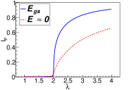
Figure 1: IPR for two different eigenvalues of the Aubry-André Hamiltonian with nearest-neighbor hopping, with $L=1000$ sites, and $\lambda$ in units of $t_{1}$.

III Two coupled chains

Let us now consider two copies of the Aubry-André chain coupled together by some additional transverse hopping parameters. The general form of the Hamiltonian is the following

$$\mathcal{H}=\sum_{i\neq j}\left(t_{ij}{\hat{c}}^{\dagger}_{i}\hat{c}_{j}+t_{ij}{\hat{d}}^{\dagger}_{i}\hat{d}_{j}\right)+\sum_{i\neq j}t^{d}_{ij}\left({\hat{c}}^{\dagger}_{i}\hat{d}_{j}+{\hat{d}}^{\dagger}_{j}\hat{c}_{i}\right)$$

$$+\sum_{i}t^{d}_{0}\left({\hat{c}}^{\dagger}_{i}\hat{d}_{i}+{\hat{d}}^{\dagger}_{i}\hat{c}_{i}\right)+\sum_{i}\epsilon(i)\left({\hat{c}}^{\dagger}_{i}\hat{c}_{i}+{\hat{d}}^{\dagger}_{i}\hat{d}_{i}\right)$$ (6)

where $\epsilon(i)=\lambda\cos(2\pi\tau i)$ are the on-site energies, $t_{ij}$ the hopping parameter between sites of the same chain, $t^{d}_{ij}$ and $t^{d}_{0}$ are the hopping parameters between sites belonging to different chains and with different or same on-site energies respectively, $\hat{c}$ and $\hat{d}$ are the operators defined on the two different chains. In the following subsections we will study numerically and analytically the localization transitions for this system.

III.1 Nearest-neighbor hopping

We first review the system of two chains coupled by nearest-neighbor hopping, introduced in Ref. Sil2008 and commented on in Ref. Flach2014 . This model is described by Fig. 2.

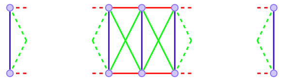
Figure 2: Two coupled chains: the red line describes the nearest-neighbor intra-chain hopping $t_{1}$, the blue line the transverse hopping $t^{d}_{0}$, the green line the nearest-neighbor inter-chain hopping $t^{d}_{1}$.

In terms of the spinor

$$\hat{b}=\left(\begin{matrix}\hat{c}\\ \hat{d}\end{matrix}\right)\,,$$ (7)

the Hamiltonian can be written

$$\mathcal{H}=\sum_{i}{\hat{b}}^{\dagger}_{i}{\cal{E}}(i)\hat{b}_{i}+\sum_{i}\left({\hat{b}}^{\dagger}_{i}{T_{1}}\,\hat{b}_{i+1}+{\hat{b}}^{\dagger}_{i+1}{T_{1}}\,\hat{b}_{i}\right),$$ (8)

where

$${\cal E}(i)=\left(\begin{matrix}\epsilon(i)&t^{d}_{0}\\ t^{d}_{0}&\epsilon(i)\end{matrix}\right)$$ (9)

and

$$T_{1}=\left(\begin{matrix}t_{1}&t^{d}_{1}\\ t^{d}_{1}&t_{1}\end{matrix}\right),$$ (10)

where $t_{1}=t_{i,i\pm 1}$ is the nearest-neighbor hopping between the $i$-th and the $(i\pm 1)$-th site of the same chain, $t^{d}_{0}$ is the transverse nearest-neighbor inter-chain hopping between the two chains and $t^{d}_{1}=t^{d}_{i,i\pm 1}$ is the nearest-neighbor inter-chain hopping between the $i$-th and the $(i\pm 1)$-th site of the two different chains (actually, it is already a next-nearest-neighbor hopping parameter between the two neighboring chains). Introducing the wavefunction

$$\Psi_{n,i}=\left(\begin{matrix}\psi^{(1)}_{n,i}\\ \psi^{(2)}_{n,i}\end{matrix}\right)$$ (11)

where $\psi^{(\alpha)}_{n,i}$ are the amplitudes of the wavefunctions at the $i$-th site of the $\alpha$-th chain ($\alpha=1,2$). The Schrödinger equation in this basis, can be written as

$$\left(E_{n}\mathbb{1}-{\cal E}(i)\right){\Psi}_{n,i}=T_{1}\left(\Psi_{n,i+1}+\Psi_{n,i-1}\right)$$ (12)

which explicitly corresponds to the following coupled equations

$$\big{(}E_{n}-\epsilon(i)\big{)}\psi^{(1)}_{n,i}-t^{d}_{0}\psi^{(2)}_{n,i} = t_{1}\big{(}\psi^{(1)}_{n,i+1}+\psi^{(1)}_{n,i-1}\big{)}$$ (13)

$$+ t^{d}_{1}\big{(}\psi^{(2)}_{n,i+1}+\psi^{(2)}_{n,i-1}\big{)}$$

$$\big{(}E_{n}-\epsilon(i)\big{)}\psi^{(2)}_{n,i}-t^{d}_{0}\psi^{(1)}_{n,i} = t_{1}\big{(}\psi^{(2)}_{n,i+1}+\psi^{(2)}_{n,i-1}\big{)}$$ (14)

$$+ t^{d}_{1}\big{(}\psi^{(1)}_{n,i+1}+\psi^{(1)}_{n,i-1}\big{)}$$

Applying the following canonical transformation

$$\psi_{n,i}^{\pm}=\frac{\psi^{(1)}_{n,i}\pm\psi^{(2)}_{n,i}}{\sqrt{2}}$$ (15)

the system is exactly mapped to two uncoupled Aubry-André chains described by Eq. (4), explicitly,

$$[E_{n}-(\epsilon(i)-t^{d}_{0})]\psi_{n,i}^{-}=(t_{1}-t^{d}_{1})(\psi_{n,i+1}^{-}+\psi_{n,i-1}^{-}),$$ (16)

$$[E_{n}-(\epsilon(i)+t^{d}_{0})]\psi_{n,i}^{+}=(t_{1}+t^{d}_{1})(\psi_{n,i+1}^{+}+\psi_{n,i-1}^{+}).$$ (17)

The full spectrum $E_{m}$ is composed by two different spectra $E_{n}^{-}=E_{n}+t^{d}_{0}$ and $E_{n}^{+}=E_{n}-t^{d}_{0}$ of two uncoupled Aubry-Andrè chains whose localization transitions occur at

$$\lambda^{+}_{c}=2(t_{1}+t^{d}_{1})$$ (18)

$$\lambda^{-}_{c}=2(t_{1}-t^{d}_{1})$$ (19)

and can be sorted in ascending order labeling $m=1,\dots,2L$, so that, for $t^{d}_{0}>0$, $E_{0}-t^{d}_{0}\leq E_{m}\leq E_{L}+t^{d}_{0}$. The corresponding eigenstates $\psi_{m,i}$ are equal to some $\psi^{+}_{n,i}$ or $\psi^{-}_{n,i}$ depending on the energy level. In particular, for $\lambda$ between the two critical values, the eigenstates $\psi_{m}$ are localized or delocalized depending on whether they correspond to $\psi^{-}_{n}$ or $\psi^{+}_{n}$. This argument can explain Fig. 3 where the IPR, $I_{P}^{(m)}=\sum_{i}|\psi_{m,i}|^{4}/\sum_{i}|\psi_{m,i}|^{2}$, is shown, in logarithmic scale, as a function of $\lambda$ and energy. Below $\lambda_{c}^{-}$ all states are delocalized, above $\lambda_{c}^{+}$ are all localized and in between, in an intermediate phase, they coexist. In Fig. 3, in the plot below, the two spectra $E^{+}$ and $E_{-}$ of the two effective chains are reported for a specific value of $\lambda$. Since there is a shift of $2t^{d}_{0}$ the nature of the states at the external bands is dictated only by one of the two effective Aubry-André chains. In this situation it is questionable speaking about the presence of a mobility edge, as explained in Ref. Flach2014 . As final remark, one can notice that for the pure ladder configuration, with $t^{d}_{1}=0$, the two effective uncoupled chains differ only by an energy shift while the critical values are the same as they are without any coupling.

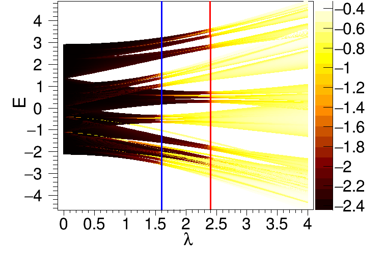
Figure 3: Inverse participation ratio (IPR), in $10$-base logarithmic scale, for two coupled Aubry-André chains with $L=200$ sites each and with nearest-neighbor hopping $t_{1}=1$, $t^{d}_{1}=0.2$ and $t^{d}_{0}=0.5$. The two vertical lines are given by Eq. (18) (red right line) and Eq. (19) (blue left line). (Below) Energy spectra, $E^{+}$ and $E^{-}$, of the two effective decoupled chains at $\lambda=\lambda_{c}^{-}=1.6$.

III.2 Generalization to longer range hopping and the case with next-nearest neighbors

We can generalize the previous results to many-neighbor hopping parameter. The Hamiltonian can be written as:

$$\mathcal{H}=\sum_{i}{\hat{b}}^{\dagger}_{i}{\cal E}(i)\hat{b}_{i}+\sum_{i,\ell}\left({\hat{b}}^{\dagger}_{i}T_{\ell}\hat{b}_{i+\ell}+{\hat{b}}^{\dagger}_{i+\ell}T_{\ell}\hat{b}_{i}\right)$$ (20)

where now $T_{\ell}$ is defined by

$$T_{\ell}=\left(\begin{matrix}t_{\ell}&t^{d}_{\ell}\\ t^{d}_{\ell}&t_{\ell}\end{matrix}\right)$$ (21)

and $t_{\ell}=t_{i,i\pm\ell}$, $t^{d}_{\ell}=t^{d}_{i,i\pm\ell}$ are the $\ell$-th-neighbor hopping terms for the sites belonging to the same chain and to different chains respectively. Introducing the wavefunction and by the transformation (15), in the same way as before, one gets two decoupled Schrödinger equations

$$\big{[}E_{n}-(\epsilon(i)+t^{d}_{0})\big{]}\psi_{n,i}^{+}=\sum_{\ell}(t_{\ell}+t^{d}_{\ell})(\psi_{n,i+\ell}^{+}+\psi_{n,i-\ell}^{+})\;\;$$ (22)

$$\big{[}E_{n}-(\epsilon(i)-t^{d}_{0})\big{]}\psi_{n,i}^{-}=\sum_{\ell}(t_{\ell}-t^{d}_{\ell})(\psi_{n,i+\ell}^{-}+\psi_{n,i-\ell}^{-})\;\;$$ (23)

describing two uncoupled extended Aubry-André models.

III.2.1 Next-nearest-neighbor hopping

Let us consider the case with second-nearest-neighbor hopping, that can be described in Fig. 4

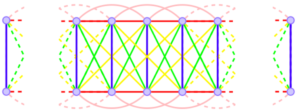
Figure 4: Two coupled chains: the red line describes the nearest-neighbor hopping $t_{1}$, the pink line the second-nearest-neighbor hopping $t_{2}$, the blue line the transverse hopping $t^{d}_{0}$, the green line the nearest-neighbor inter-chain hopping $t^{d}_{1}$, the yellow line the second-nearest-neighbor inter-chain hopping $t^{d}_{2}$.

so that Eqs. (22), (23) becomes simply

$$\big{[}E_{n}-(\epsilon(i)-t^{d}_{0})\big{]}\psi_{n,i}^{-}=(t_{1}-t^{d}_{1})(\psi_{n,i+1}^{-}+\psi_{n,i-1}^{-})$$

$$+(t_{2}-t^{d}_{2})(\psi_{n,i+2}^{-}+\psi_{n,i-2}^{-})$$ (24)

$$\big{[}E_{n}-(\epsilon(i)+t^{d}_{0})\big{]}\psi_{n,i}^{+}=(t_{1}+t^{d}_{1})(\psi_{n,i+1}^{+}+\psi_{n,i-1}^{+})$$

$$+(t_{2}+t^{d}_{2})(\psi_{n,i+2}^{+}+\psi_{n,i-2}^{+})$$ (25)

which are two uncoupled chains. In the hypothesis of $(t_{2}\pm t^{d}_{2})\ll(t_{1}\pm t^{d}_{1})$ and neglecting further terms which can be assumed exponentially small, we can resort to the analytical result reported in Eq. (3) for a single extended Aubry-André model Biddle ; Ramakumar2014 , getting the following values of the critical potentials

$$\lambda^{-}_{c}=\frac{2(t_{1}-t^{d}_{1})+2(E_{n}+t^{d}_{0})\left(\frac{t_{2}-t^{d}_{2}}{t_{1}-t^{d}_{1}}\right)}{1+\left(\frac{t_{2}-t^{d}_{2}}{t_{1}-t^{d}_{1}}\right)^{2}}$$ (26)

$$\lambda^{+}_{c}=\frac{2(t_{1}+t^{d}_{1})+2(E_{n}-t^{d}_{0})\left(\frac{t_{2}+t^{d}_{2}}{t_{1}+t^{d}_{1}}\right)}{1+\left(\frac{t_{2}+t^{d}_{2}}{t_{1}+t^{d}_{1}}\right)^{2}}$$ (27)

As one can see from Fig. 5, the full spectrum results from the overlap of the spectra of two uncoupled chains so that in general one can have an intermediate phase defined as a regime of parameters for which we have a coexistence of localized and delocalized states.

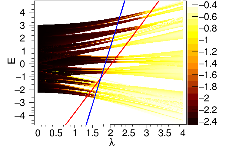
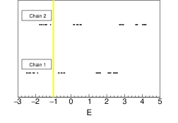
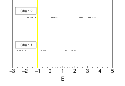
Figure 5: Inverse participation ratio (IPR), in $10$-base logarithmic scale, for two coupled Aubry-André chains ($L=200$) with second-nearest-neighbor hopping: $t_{1}=1$, $t^{d}_{1}=0.1$, $t_{2}=0.1$, $t^{d}_{2}=0.05$ and $t^{d}_{0}=0.5$. The lines are given by Eq. (26) (blue line) and Eq. (27) (red line) in clockwise order. (Below) Energy spectra, $E^{+}$ and $E^{-}$, of the two effective decoupled chains along $\lambda=\lambda^{+}_{c}$ (upper plot) and $\lambda=\lambda^{-}_{c}$ (lower plot). The yellow vertical line indicates the crossing energy point $E^{*}$.

For the sake of simplicity of notation let us define

$$A_{+}=\frac{t_{2}+t^{d}_{2}}{t_{1}+t^{d}_{1}}$$ (28)

$$A_{-}=\frac{t_{2}-t^{d}_{2}}{t_{1}-t^{d}_{1}}$$ (29)

As shown in Fig. 5, the localized and delocalized states are delimited by the transition lines defined by Eqs. (26), (27) which are straight lines as functions of the energy with slopes $2A_{\pm}/(1+A_{\pm}^{2})$. In order to determine the crossing point one can impose the condition $\lambda^{+}_{c}=\lambda^{-}_{c}$ and solve the equation for the energy, getting

$$E^{*}=\frac{1}{(A_{+}-A_{-})(1-A_{+}A_{-})}\Big{[}t^{d}_{0}(1+A_{+}A_{-})(A_{+}+A_{-})$$

$$\phantom{E^{*}=}-t^{d}_{1}(2+A_{+}^{2}+A_{-}^{2})+t_{1}(A_{+}^{2}-A_{-}^{2})\Big{]}$$ (30)

for $A_{+}\neq A_{-}$ and $A_{+}\neq 1/A_{-}$, as shown in Fig. 5. On the other hand, if $A_{+}=A_{-}$ (or $A_{+}=1/A_{-}$), the two lines are parallel as in the case of Fig. 7. The most relevant physical situation is when $A_{+}=A_{-}$ (in agreement with the hypothesis $t_{2}\pm t_{2}^{d}\ll t_{1}\pm t_{1}^{d}$), namely when

$$\frac{t_{1}}{t_{2}}=\frac{t^{d}_{1}}{t^{d}_{2}}.$$ (31)

By this condition we have two parallel critical lines with slope $\frac{2(t_{2}/t_{1})}{1+\left(t_{2}/t_{1}\right)^{2}}$ and a coexisting region where there are localized and delocalized states, as show in Fig. 6. If we now impose an additional condition to Eq. (31) for the hopping parameters

$$\frac{t^{d}_{0}}{t^{d}_{1}}=\frac{t_{1}}{t_{2}}$$ (32)

which is also quite reasonable, we get that $\lambda^{+}_{c}=\lambda^{-}_{c}$ for any value of the energy. From Eqs. (31) and (32) we can express the critical potential in terms of only $t_{1}/t_{2}$, getting the same result as that of a single chain with exponentially short-range hopping, Eq. (3). This means that we get a uniquely defined mobility edge which separates the localized phase from the delocalized one, as shown in Fig. 7. The above results, to our knowledge, have not been presented before.

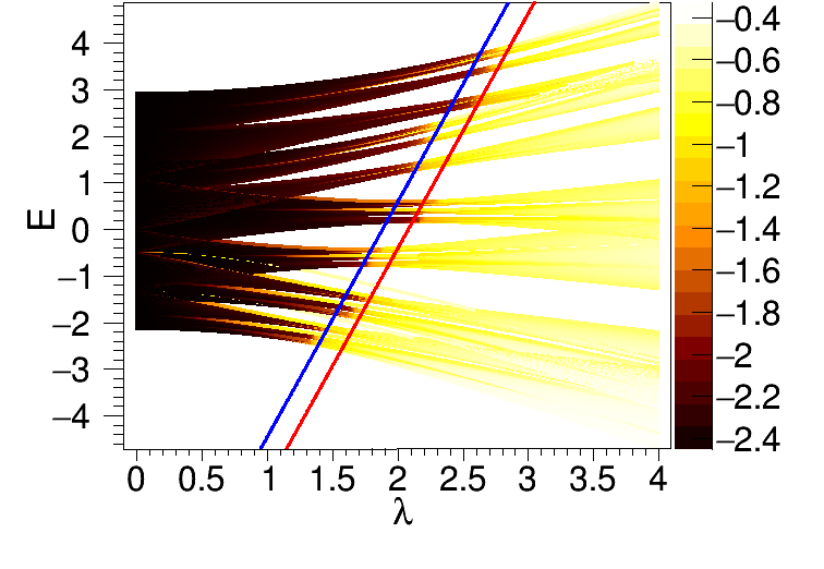
Figure 6: Inverse participation ratio (IPR), in $10$-base logarithmic scale, for two coupled Aubry-André chains ($L=200$) with second-nearest-neighbor hopping: $t_{1}=1$, $t^{d}_{1}=0.1$, $t_{2}=0.1$, $t^{d}_{2}=0.01$ and $t^{d}_{0}=0.5$. The lines are described by Eq. (26) (blue left line) and Eq. (27) (red right line). (Below) Energy spectra, $E^{+}$ and $E^{-}$, of the two effective decoupled chains along $\lambda=\lambda^{-}_{c}$.

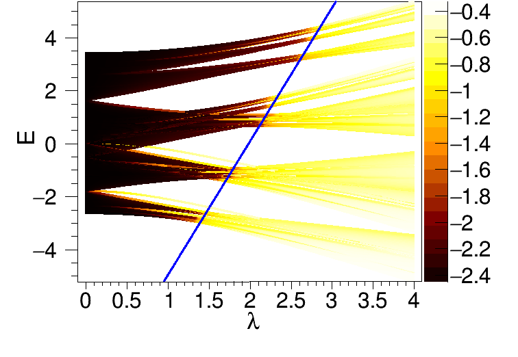
Figure 7: Inverse participation ratio (IPR), in $10$-base logarithmic scale, for two coupled Aubry-André chains ($L=200$) with second-nearest-neighbor hopping: $t_{1}=1$, $t^{d}_{1}=0.1$, $t_{2}=0.1$, $t^{d}_{2}=0.01$ and $t^{d}_{0}=1$. Since Eqs. (31), (32) are fulfilled, so that the critical line can be written in terms of only the ratio $t_{1}/t_{2}$, the mobility edge, described by the blue straight line, is given by Eq. (3). (Below) Energy spectra, $E^{+}$ and $E^{-}$, of the two effective decoupled chains along $\lambda=\lambda^{-}_{c}=\lambda^{+}_{c}$.

III.3 Intermediate phase: coexistence of extended and localized states

We can define two different quantities that draw the contour of the region of parameters where localized and delocalized states coexist Li2017 .
From the definition of IPR for an arbitrary state, Eq. (5), we can take the average over a set of energy levels whose number is $N_{L}$

$$\left\langle{I_{P}}\right\rangle=\sum_{n}^{N_{L}}\frac{I_{P}^{(n)}}{N_{L}}$$ (33)

which vanishes when all the $N_{L}$ states are extended. One can use also a complementary quantity, the normalized participation ratio (NPR)

$$N_{P}^{(n)}=\frac{1}{L\sum_{i}|\psi_{n,i}|^{4}}$$ (34)

and, analogously, from that, one defines its average over a subset of states,

$$\left\langle{N_{P}}\right\rangle=\sum_{n}^{N_{L}}\frac{N_{P}^{(n)}}{N_{L}}$$ (35)

where $L$ is the size of the system, which vanishes when all the $N_{L}$ states are localized.
In the regime where both $\left\langle{I_{P}}\right\rangle$ and $\left\langle{N_{P}}\right\rangle$ remain finite, the spectrum of the Hamiltonian allows for a phase which has both spatially extended and localized eigenstates. This behavior defines an intermediate phase (the shaded regions in Fig. 8) made by a mixture of extended and localized states.

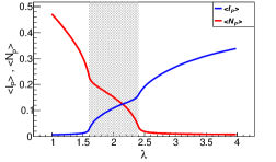
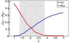
Figure 8: The averaged IPR and NPR, $\left\langle{I_{P}}\right\rangle$ and $\left\langle{N_{P}}\right\rangle$, obtained from the spectrum reported in Fig. 3 (nearest-neighbor case) and in Fig. 6 (next-nearest-neighbor case).

In Fig. 8 we plotted $\left\langle{I_{P}}\right\rangle$ and $\left\langle{N_{P}}\right\rangle$ got from averaging over all the eigenstates, for nearest-neighbor and next-nearest-neighbor cases of two coupled Aubry-André models. This intermediate phase can be detected also dynamically, as shown in Refs. r3 ; Luschen2017 , measuring a finite density imbalance between even and odd sites due to an initial charge density wave state persisting in time.

IV Many coupled chains: square lattice with quasi-periodicity in one direction

Let us now consider a further generalization, coupling $S$ identical Aubry-André chains, as in Ref. Guo , so that the system is described by the following Hamiltonian

$$\mathcal{H}=\sum_{i\neq j,\alpha}t_{ij}{\hat{c}}^{\dagger}_{i,\alpha}\hat{c}_{j,\alpha}+{\color[rgb]{0,0,0}\frac{1}{2}}\sum_{i\neq j,\alpha\neq\beta}t^{d}_{ij,\alpha\beta}\left({\hat{c}}^{\dagger}_{i,\alpha}\hat{c}_{j,\beta}+{\hat{c}}^{\dagger}_{j,\beta}\hat{c}_{i,\alpha}\right)$$

$$+{\color[rgb]{0,0,0}\frac{1}{2}}\sum_{i,\alpha\neq\beta}t^{d}_{0,\alpha\beta}\left({\hat{c}}^{\dagger}_{i,\alpha}\hat{c}_{i,\beta}+{\hat{c}}^{\dagger}_{i,\beta}\hat{c}_{i,\alpha}\right)+\sum_{i,\alpha}\epsilon(i){\hat{c}}^{\dagger}_{i,\alpha}\hat{c}_{i,\alpha}$$ (36)

For simplicity, we will consider only couplings between nearest-neighbor chains, namely $\sum_{\alpha\neq\beta}$ represents $\sum_{\langle\alpha,\beta\rangle}$, a sum over nearest-neighbor chains, so that we can keep using the same notation as before, $t^{d}_{0}\equiv t^{d}_{0,\alpha\,\alpha\pm 1}$ and $t^{d}_{ij}\equiv t^{d}_{ij,\alpha\,\alpha\pm 1}$, where $t^{d}_{i\,i\pm\ell}=t^{d}_{\ell}$. By these definitions, the Hamiltonian can be rewritten as in Eq. (20) where now

$$\hat{b}_{i}=\left(\begin{matrix}\hat{c}_{i,1}\\ \vdots\\ \hat{c}_{i,S}\end{matrix}\right)$$ (37)

and the $S\times S$ matrices

$${\cal E}(i)=\left(\begin{matrix}\epsilon(i)&t^{d}_{0}&0&\dots&0\\ t^{d}_{0}&\epsilon(i)&t^{d}_{0}&\ddots&\vdots\\ 0&t^{d}_{0}&\epsilon(i)&\ddots&0\\ \vdots&\ddots&\ddots&\ddots&t^{d}_{0}\\ 0&\dots&0&t^{d}_{0}&\epsilon(i)\\ \end{matrix}\right)$$ (38)

and

$$T_{\ell}=\left(\begin{matrix}t_{\ell}&t^{d}_{\ell}&0&\dots&0\\ t^{d}_{\ell}&t_{\ell}&t^{d}_{\ell}&\ddots&\vdots\\ 0&t^{d}_{\ell}&t_{\ell}&\ddots&0\\ \vdots&\ddots&\ddots&\ddots&t^{d}_{\ell}\\ 0&\dots&0&t^{d}_{\ell}&t_{\ell}\\ \end{matrix}\right)$$ (39)

The matrices ${\cal E}(i)$ and $T_{\ell}$ can be diagonalized simultaneously by the same unitary transformation and the eigenvalues are $\epsilon(i)+t_{0}^{d}\varepsilon(k)$ and $t_{\ell}+t^{d}_{\ell}\varepsilon(k)$ respectively, where

$$\varepsilon(k)=2\cos\left(\frac{\pi k}{S+1}\right)$$ (40)

Notice that we are considering a planar geometry, namely the coupling of the chains is open at the boundary. If we consider instead periodic boundary condition, namely the first and the last chains are coupled, the matrices Eqs. (38), (39) would have had elements $t^{d}_{0}$ and $t^{d}_{\ell}$ respectively at the right-top and bottom-left corners. In that case Eq. (40) should be replaced by $\varepsilon(k)=2\cos\left(\frac{2\pi k}{S}\right)$. The $S$-chains model, therefore, can be decoupled to $S$ Aubry-André chains, labeled by the index $k=1,\dots S$, that satisfy the following eigenvalue equations

$$\big{[}E_{n}-\epsilon(i)-t^{d}_{0}\,\varepsilon(k)\big{]}\psi^{k}_{n,i}$$ (41)

$$\phantom{----}=\sum_{\ell}\left(t_{\ell}+t^{d}_{\ell}\,\varepsilon(k)\right)\left(\psi^{k}_{n,i+\ell}+\psi^{k}_{n,i-\ell}\right).$$

In the case of several coupled chains a clarification about the localization phase is in order. The system can be considered as two-dimensional with size $S\times L$, and since in the direction of the array of the chains, let us call it $y$-direction, the couplings are due to homogeneous hopping parameters, the localization of the wavefunctions induced by the quasiperiodic potential can occur only along the direction of the Aubry-Andrè chains, $x$-direction. As a result, for finite systems, the IPR of a generic $n$-th normalized eigenstate will be limited by

$$\frac{1}{SL}<I_{P}^{(n)}\lesssim\frac{1}{S},$$ (42)

more precisely, for open boundary conditions, $I_{P}^{(n)}<\frac{3}{2S}$.

IV.1 Nearest-neighbor hopping

Let us consider the nearest-neighbor hopping case ($j=i\pm 1$) depicted in Fig. 9.

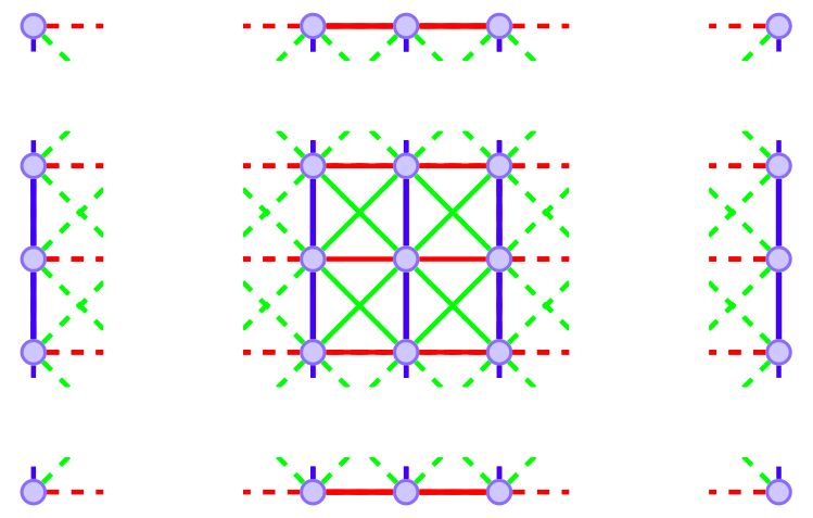
Figure 9: Many coupled chains: the red line describes the nearest-neighbor intra-chain hopping $t_{1}$, the blue line the transverse inter-chain hopping $t^{d}_{0}$, the green line nearest-neighbor inter-chain hopping $t^{d}_{1}$.

The $S$ effective uncoupled Aubry-André chains have the following critical potentials

$$\lambda^{k}_{c}=2\left(t_{1}+t^{d}_{1}\,\varepsilon(k)\right)$$ (43)

As shown in Fig. 10, the critical potentials divide the phase diagram into three regions.

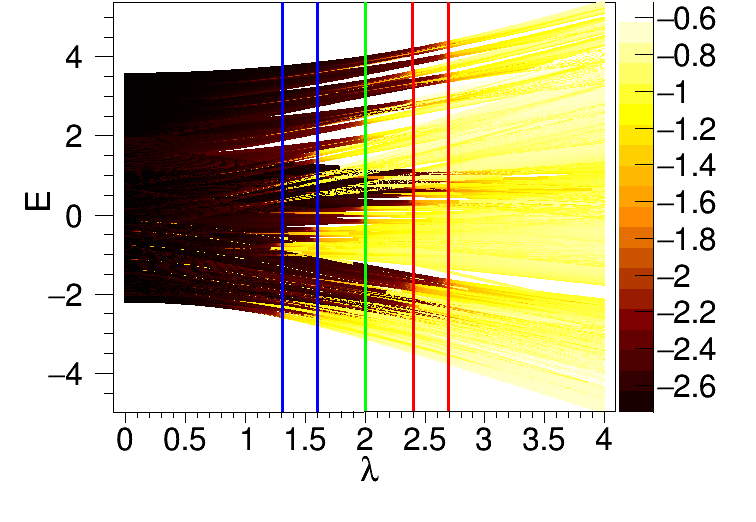
Figure 10: Inverse participation ratio (IPR), in $10$-base logarithmic scale, for $S=5$ coupled Aubry-Andé chains ($L=200$) with nearest-neighbor hopping $t_{1}=1$, $t^{d}_{1}=0.2$, and $t^{d}_{0}=0.5$. The vertical lines are described by Eq. (43), with $k=1,\dots,S$, from right (red line) to left (blue line).

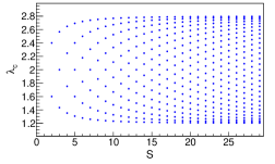
Figure 11: Critical amplitudes of the effective uncoupled Aubry-André chains, Eq. (43), for different numbers $S$ of originally coupled chains, for $t_{1}=1$ and $t^{d}_{1}=0.2$.

For $\lambda<\lambda^{S}_{c}$ all the eigenstates are extended while for $\lambda>\lambda^{1}_{c}$ are all localized. For $\lambda^{S}_{c}<\lambda<\lambda^{1}_{c}$, instead, there is an intermediate region where localized and extended states coexist. This region increases with the number of chains but is delimited by $t_{1}-2t^{d}_{1}<\lambda<t_{1}+2t^{d}_{1}$, as shown in Fig. 11.

IV.2 Next-nearest-neighbor hopping

Let us now consider next-nearest-neighbor hopping terms (Fig. 12), supposing that further terms are exponentially small. In this case, after decoupling the chains we get the following $S$ critical Aubry-André amplitudes

$$\lambda^{k}_{c}=\frac{2\left(t_{1}+t^{d}_{1}\,\varepsilon(k)\right)+2\left(E_{n}-t^{d}_{0}\,\varepsilon(k)\right)A_{k}}{1+A^{2}_{k}}$$ (44)

where

$$A_{k}=\frac{t_{2}+t^{d}_{2}\,\varepsilon(k)}{t_{1}+t^{d}_{1}\,\varepsilon(k)}$$ (45)

These expressions are the generalization of Eqs. (26)-(29), already seen for two chains. Examples of the transitions obtained for three and five coupled Aubry-André chains are given in Fig. 13.

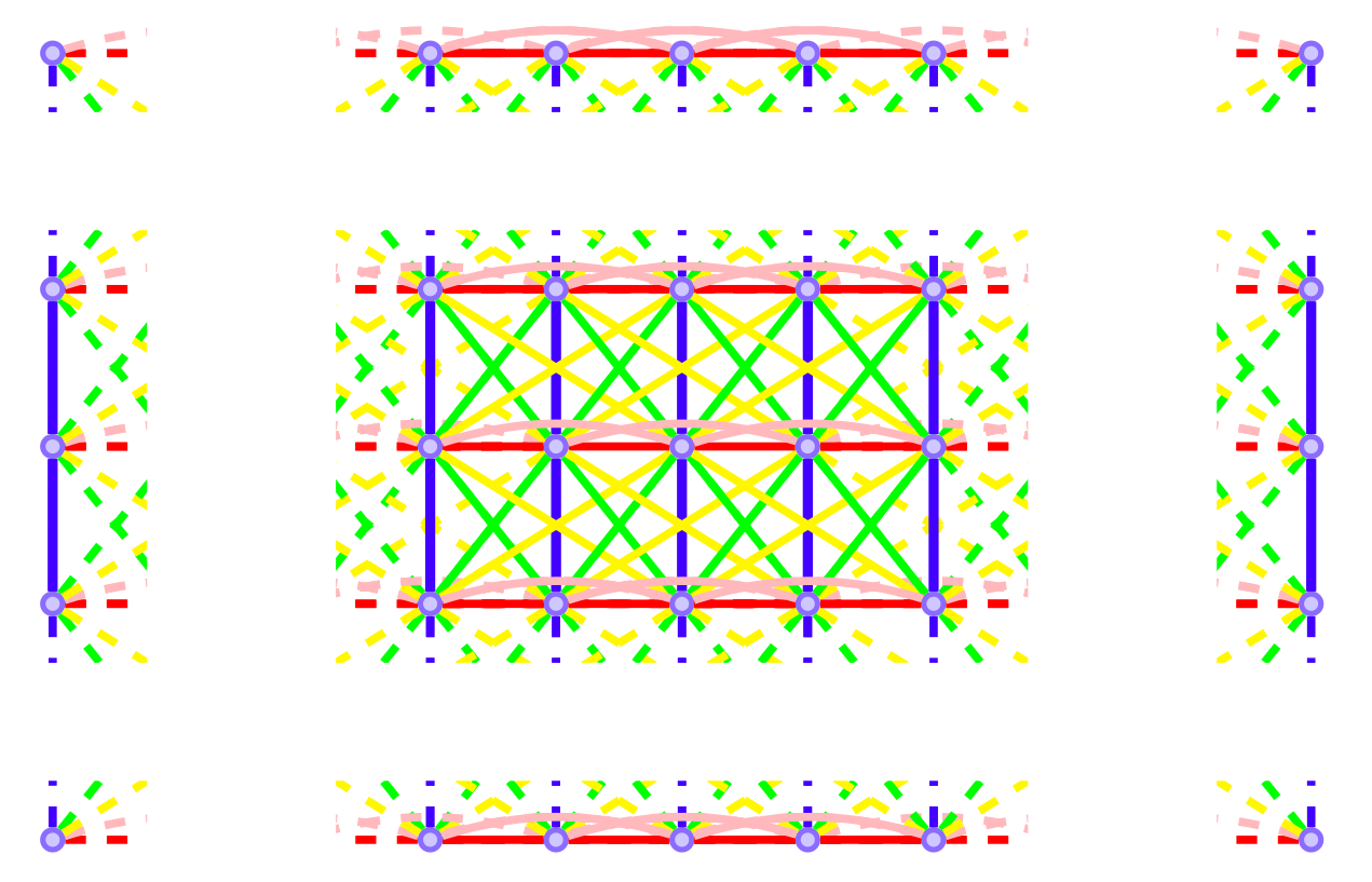
Figure 12: Many coupled chains: the red line describes the nearest-neighbor intra-chain hopping $t_{1}$, the blue line the transverse inter-chain hopping $t^{d}_{0}$, the green line nearest-neighbor inter-chain hopping $t^{d}_{1}$, the pink line the next-nearest-neighbor hopping $t_{2}$, the yellow line the inter-chain hopping $t^{d}_{2}$.

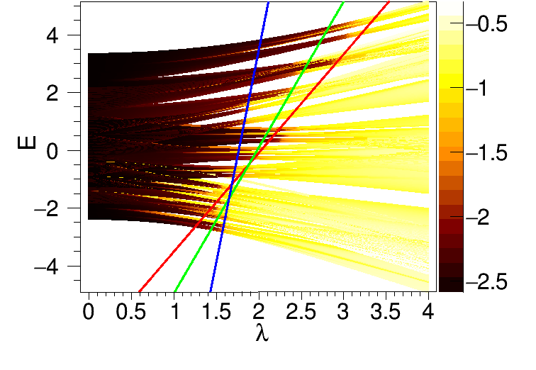
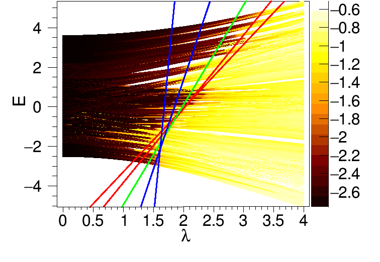
Figure 13: Inverse participation ratio (IPR), in $10$-base logarithmic scale, for $S=3$ and $S=5$ coupled Aubry-Andé chains ($L=200$) with next-nearest-neighbor hopping parameters $t_{1}=1$, $t_{2}=t^{d}_{1}=0.1$, $t^{d}_{2}=0.05$ and $t^{d}_{0}=0.5$. The straight lines are given by Eq. (44), with $k=1,\dots,S$, from red to blue lines in a counterclockwise order.

If we now impose the condition $\lambda^{k}_{c}=\lambda^{k^{\prime}}_{c}$, solving this equation in terms of the energy we get

$$E^{*}=\frac{1}{(A_{k^{\prime}}-A_{k})(1-A_{k^{\prime}}A_{k})}\big{[}(1+A_{k^{\prime}}^{2})(t^{d}_{1}-A_{k}t^{d}_{0})\varepsilon(k)$$

$$\phantom{--}-(1+A_{k}^{2})(t^{d}_{1}-A_{k^{\prime}}t^{d}_{0})\varepsilon(k^{\prime})+t_{1}(A_{k^{\prime}}^{2}-A_{k}^{2})\big{]}$$ (46)

For all $k$ and $k^{\prime}$ such that $(A_{k^{\prime}}-A_{k})(1-A_{k^{\prime}}A_{k})\neq 0$, we can get $\frac{S(S-1)}{2}$ different solutions $E^{*}$ (see for instance Fig. 13). If, otherwise, $A_{k}=A_{k^{\prime}}$ or equivalently, in terms of the hopping parameters, $t_{1}t^{d}_{2}=t_{2}t^{d}_{1}$, which is the same condition as before, reported in Eq. (31), all the straight lines described by Eq. (44) have the same slope, independently from $k$, that is $\frac{2t_{2}/t_{1}}{1+\left(\frac{t_{2}}{t_{1}}\right)^{2}}$. If we now impose a further condition, $t^{d}_{0}=\frac{t^{d}_{1}}{t_{2}}t_{1}$, Eq. (32), all the parallel lines overlap each other as shown in Fig. 14 and we get a unique mobility edge, expressed again by Eq. (3), dividing the extended states from the localized ones in the $x$-direction.

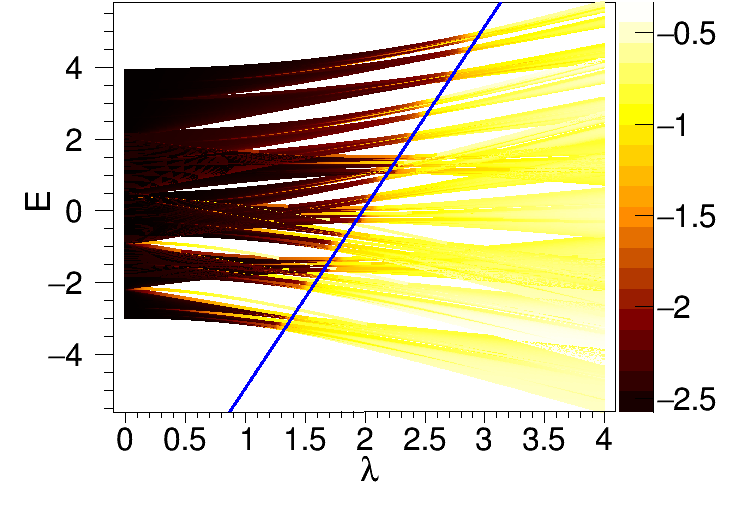
Figure 14: Inverse participation ratio (IPR), in $10$-base logarithmic scale, for $S=3$ coupled Aubry-Andé chains ($L=200$) with next-nearest-neighbor hopping parameters $t_{1}=1$, $t^{d}_{1}=t_{2}=0.1$, $t^{d}_{2}=0.01$, $t^{d}_{0}=1$. Since Eqs. (31), (32) are fulfilled, so that the critical line can be written in terms of only the ratio $t_{1}/t_{2}$, the mobility edge, described by the blue straight line, is given by Eq. (3).

IV.3 Long-range hopping among the chains

A further generalization of what seen so far can be obtained allowing for longer-range coupling among the chains, although the physics is qualitatively the same as that seen in the last case. Imposing for simplicity periodic boundary conditions in the transverse direction, namely, along the array of the chains, assuming an exponential decay of the hopping terms, Eq. (44) should be replaced by

$$\lambda^{k}_{c}=\frac{2\left(t_{1}+{\cal P}_{1}(k)\right)+2\left(E_{n}-{\cal P}_{0}(k)\right)A_{k}}{1+A^{2}_{k}}$$ (47)

where now $A_{k}$ is also replaced by

$$A_{k}=\frac{t_{2}+{\cal P}_{2}(k)}{t_{1}+{\cal P}_{1}(k)}$$ (48)

depending on the spectrum along the transverse direction

$${\cal P}_{\ell}(k)=2\sum_{\gamma=1}^{S-1}t^{d}_{\ell,\gamma}\cos(2\pi\gamma k/S).$$ (49)

It is worth remembering that the validity of Eq. (47) is based on the assumtion that $\left(t_{\ell}+{\cal P}_{\ell}(k)\right)$ decays exponentially with $\ell$, so that $A_{k}$ in Eq. (48) is the exponential factor. Referring to the Hamiltonian in Eq. (36), the hopping parameters are defined by $t^{d}_{0,\gamma}=t^{d}_{0,\alpha\,\alpha\pm\gamma}$ and $t^{d}_{\ell,\gamma}=t^{d}_{i\,i\pm\ell,\alpha\,\alpha\pm\gamma}$. Also in this case, imposing the condition $\lambda_{c}^{k}=\lambda_{c}^{k^{\prime}}$ we get the crossing points as in Eq. (46), where the terms $t_{\ell}^{d}\varepsilon(k)$ are replaced by ${\cal P}_{\ell}(k)$, in the hypothesis of a non-vanishing denominator.
If, instead we impose $A_{k}=A_{k^{\prime}}$, for any $k$ and $k^{\prime}$, we get the condition

$$\frac{t_{1}}{t_{2}}=\frac{t^{d}_{1,\gamma}}{t^{d}_{2,\gamma}},\;\;\,\forall\,\gamma\,,$$ (50)

as in Eq. (31), so that $A_{k}=t_{2}/t_{1}$ drops the $k$-dependence. In this condition, requiring $\lambda_{c}^{k}=\lambda_{c}^{k^{\prime}}$, we obtain

$$\frac{t_{1}}{t_{2}}=\frac{t^{d}_{0,\gamma}}{t^{d}_{1,\gamma}},\;\;\,\forall\,\gamma\,,$$ (51)

as in Eq. (32), which brings to have a unique mobility edge described by Eq. (3). In conclusions, also in the most general case treated here, where all the several chains are coupled together, Eq. (47) can be reduce to Eq. (3), the same mobility edge as that of a single chain with exponentially decaying hopping terms.

V 2D Aubry André model: square lattice with quasi-periodicity in both directions

Let us now consider a final further generalization, coupling (by simply transverse nearest neighbor hopping $t_{0}^{d}$) $S$ different Aubry-André chains with single-site shifted energies between two neighboring chains. For $S$ and $L$ both very large we get a generalization of the Aubry-André model in two dimensions (2D), being the quasiperiodic potential in both directions. The system is described by the following Hamiltonian

$$\mathcal{H}=\sum_{\langle i,j\rangle,\alpha}t_{1}{\hat{c}}^{\dagger}_{i,\alpha}\hat{c}_{j,\alpha}+\sum_{i,\langle\alpha,\beta\rangle}t^{d}_{0}\,{\hat{c}}^{\dagger}_{i,\alpha}\hat{c}_{i,\beta}+\sum_{i,\alpha}\epsilon(i,\alpha){\hat{c}}^{\dagger}_{i,\alpha}\hat{c}_{i,\alpha}$$ (52)

where we will consider $t_{1}=t_{0}^{d}=1$ (the same hopping in both $x$ and $y$ directions). The on-site energies are obtained by shifting the chains, namely,

$$\epsilon(i,\alpha)=\lambda\cos\left(2\pi\tau(i+\ell\alpha)\right).$$ (53)

In general one can use $\epsilon(i,\alpha)=\lambda\cos(2\pi\tau(\ell_{x}i+\ell_{y}\alpha))$, so that for $\ell_{y}=0$ and $\ell_{x}=1$, we recover the result for quasiperiodic potential in $x$-direction, as seen before, and for $\ell_{y}=1$ and $\ell_{x}=0$ the same but with the potential in $y$-direction. In these cases we have the usual critical potential, $\lambda_{c}=2t_{1}$ or $\lambda_{c}=2t_{0}^{d}$, as in the standard Aubry-André model, because of the perfect decoupling. We will consider also the case where $\ell$ is a random value which takes values $-1,0,1$, meaning that the chains are randomly shifted by at most one lattice step.
We will consider also a truly aperiodic 2D Aubry-André model using the potential

$$\epsilon(i,\alpha)=\lambda\cos(2\pi\tau i)+\lambda\cos(2\pi p\,\alpha),$$ (54)

where $p$ is an irrational number, we will take $p=\sqrt{2}$.

V.1 Two coupled chains with shift

Let us first consider two chains, which are now not identical, coupled by a simple transverse hopping $t_{0}$, and the intra-chain hopping parameter is only $t_{1}$. The energies of the first chain $\varepsilon(i,1)$ are equal to the energies of the second chain after a translation of $\ell$ sites, $\varepsilon(i,2)=\varepsilon(i+\ell,1)$ (with $\ell$ an integer number). We can rewrite the Hamiltonian as in Eq. (8) with ${\cal E}(i)=\left(\begin{matrix}\epsilon(i)&t^{d}_{0}\\ t^{d}_{0}&\epsilon(i+\ell)\end{matrix}\right)$ and $T_{1}=\left(\begin{matrix}t_{1}&0\\ 0&t_{1}\end{matrix}\right)$. Even if ${\cal E}$ and $T_{1}$ trivially commutes so that they can be diagonalized simultaneously as in the case of two identical chains, since the transformation of the fields is not global, we cannot decouple the systems into two uncoupled Aubry-André chains, as done before. Alternatively one can show that choosing a different basis the energy term is not diagonalizable, see Appendix A. We have, therefore, to resort to numerical exact diagonalization. An example of the IPR for a system of two coupled chains with $t_{1}=t_{0}^{d}$ and with shift in energies $\ell=1$ is reported in Fig. 15. It is important to note that the transition between localized and extended states depends strongly on the energy level, in contrast to what happens for identical chains ($\ell=0$) where the transition occurs at $\lambda=2t_{1}$, independently of the energy.

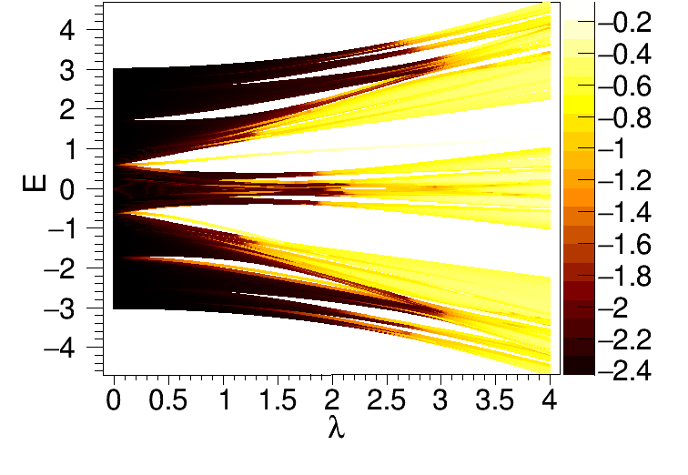
Figure 15: Inverse participation ratio (IPR), in $10$-base log-scale, for two coupled Aubry-André chains ($S=2$ and $L=200$), with single-site shifted energies, $\epsilon(i+1,1)=\epsilon(i,2)$, and with nearest-neighbor hopping $t_{1}=t^{d}_{0}=1$.

V.2 Many coupled chains with shift

We can now put together more than two chains with single-site energy shifts between nearest neighbor chains. When the number of chains $S$ is of the same order of the length of the chains $L$ we realize the generalization of the Aubry-André model in two dimensions, on a square lattice. For $t_{0}^{d}=t_{1}=1$ and $S=L=50$ the results for IPR in logarithmic scale ($\log_{10}(I_{P}^{(n)})$ for any energy levels $n$) are reported in Fig. 16. Although the IPR is expected to takes value between $1/SL$ and $1$, we observe that, even for large potential $\lambda$, the IPR is far from $1$ (its log is far from $0$) meaning that the eigenstates are far from being strongly localized.

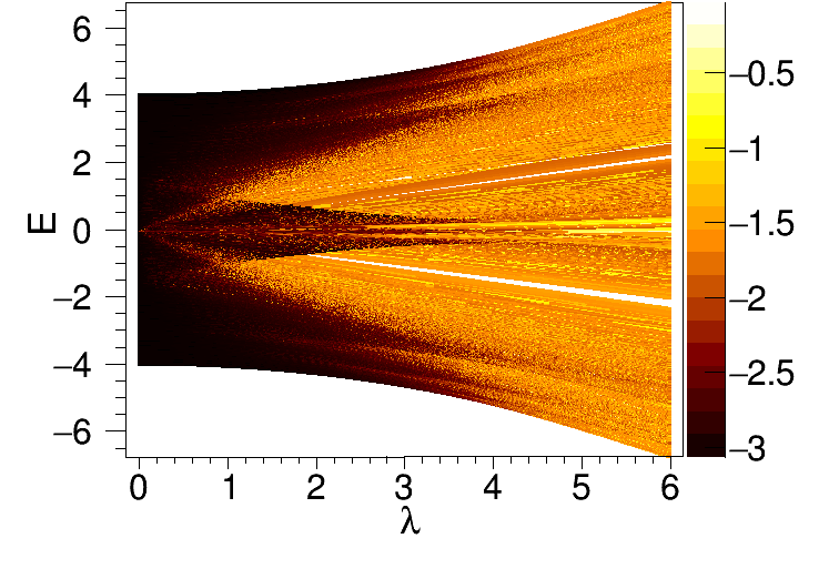
Figure 16: Inverse participation ratio (IPR), in $10$-base log-scale, for many coupled Aubry-André models, Eqs. (52), (53), with $L=S=50$, and nearest-neighbor hopping $t_{1}=t_{0}^{d}=1$.

This result suggests that, even for large quasidisorder potential, the eigenstates remain somewhat extended, with values of $I_{P}$ of order of magnitude $1/L$.
This behavior can be explained in the thermodynamic limit, for $S,L\rightarrow\infty$, where a transverse periodicity occurs, by applying the transformation $\hat{c}_{i,\alpha}=\sum_{k}e^{-\imath k(i-\alpha)}\hat{c}_{i+\alpha}(k)$, so that the Hamiltonian, Eq. (52) with Eq. (53), can be written as $\mathcal{H}=\sum_{k}\mathcal{H}_{k}$, where

$$\mathcal{H}_{k}=t(k)\sum_{i,\delta=\pm 1}{\hat{c}}^{\dagger}_{i}(k)\hat{c}_{i+\delta}(k)+\sum_{i}\epsilon(i){\hat{c}}^{\dagger}_{i}(k)\hat{c}_{i}(k)$$ (55)

with $\epsilon(i)=\lambda\cos(2\pi\tau i)$ and $t(k)=2t_{1}\cos(k)$, for $t_{1}=t_{0}^{d}$. As a result the system is decoupled to infinitely many 1D Aubry-André models labeled by the mode numbers $k$, for which the transition occurs at $\lambda=2|t(k)|$. This means that for $\lambda<4t_{1}$ we have localized and extended states while for $\lambda>4t_{1}$ we have only localized states (as clearly shown in Fig. 16), still in $(\hat{x}-\hat{y})$-direction, being the system periodic, the states remain extended. The localization is therefore only partial so that, for $L\sim S$, the IPR goes like $1/L$ for large $\lambda$ (see Fig. 18, the red curve for the average IPR).
A stronger localization can be obtained by coupling chains which are randomly shifted, namely with energies as in Eq. (53) but where $\ell$ takes random integer values. The corresponding IPR is more blurred than that of Fig. 16 while for large $\lambda$ it behaves like the IPR of the 2D Anderson model (see the violet dashed line in Fig. 18 which is the average IPR, where $\ell$ takes randomly the values $-1,0,1$, uniformly distributed).

V.3 Truly aperiodic 2D Aubry-André model

Finaly, let us consider a truly aperiodic 2D Aubry-André model, with on-site energies given by Eq. (54) (we used $p=\sqrt{2}$). In this case the system is not periodic in any directions. We calculated the eigenvalues and eigenstates numerically finding that the IPR exhibits again a sharp phase transition at $\lambda=2$ (in units of $t_{1}=t_{0}^{d}$), as one can clearly see from Fig. 17. In this case the all states are localized for $\lambda>2$ and the localization is more pronunced than that of the prevous system, made by shifted chains, and that of a 2D Anderson model, with the IPR which goes rapidly to $1$.

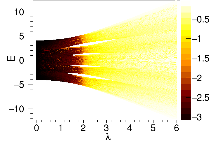
Figure 17: Inverse participation ratio (IPR), in $10$-base log-scale, for the 2D Aubry-André, with energies given by Eq. (54), with $p=\sqrt{2}$, and where $L=S=50$, and nearest-neighbor hopping $t_{1}=t_{d}=1$.

V.4 Comparison with 2D Anderson model

In order to clarify the results for the 2D Aubry-André model it is useful to make a comparison with what one might obtain if the quasidisorder were replaced by a true uncorrelated disorder, as in the 2D Anderson model. We, therefore, solve the eigenproblem for an Hamiltonian as in Eq.  (52), with $\varepsilon(i,\alpha)$ replaced by random variables uniformly distributed between $-\lambda$ and $\lambda$. The value of $\lambda$ is, therefore, the strength of disorder.

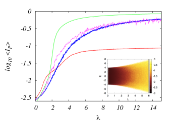
Figure 18: Average inverse participation ratio, over all the eigenstates, in $10$-base log-scale, for the generalized 2D Aubry-André model obtained by uniformly shifting the chains, Eq. (53) (red curve), for the same Aubry-André model but where the coupled chains are randomly shifted (violet dashed line), for the 2D Anderson model (blue curve), and for the truly aperiodic 2D Aubry-André model, Eq. (54) (green line). All these models are defined on a square lattice with size $L=S=30$ and nearest-neighbor hopping $t_{1}=t_{0}^{d}=1$. Inset: Inverse participation ratio, in $10$-base log scale, for the 2D Anderson model with $S=L=30$ and $t_{1}=t_{0}^{d}=1$, as function of the energy levels and $\lambda$.

In Fig. 18 we plot the average inverse participation ratio, $\langle I_{P}\rangle=\frac{1}{SL}\sum_{n=1}^{SL}I_{P}^{(n)}$, for 2D Aubry-André model obtained by coupling many chains uniformly shifted (red curve) or randomly shifted (violet dashed line), so that the potential is given by Eq. (53), or by applying an aperiodic potential like Eq. (54), so that we get a truly aperiodic 2D Aubry-André model (green line), in order to compare with the 2D Anderson model where the potential is an uncorrelated disorder (blue line). We observe that $\langle I_{P}\rangle$ depends weakly on $\lambda$, in the strong quasidisorder regime, for the system composed of shifted chains (red line). Indeed the curve is flat upon increasing $\lambda$, almost fixed at a value of the order of $1/L$. On the contrary, for the 2D Anderson model with large disorder, supposing $\langle I_{P}\rangle\sim 1/\xi^{2}$, where $\xi$ is the localization length, we find numerically that $\xi\sim e^{c/\lambda}$ (with $c\approx 5$ in units of $t_{1}=t_{0}^{d}$) in agreement with the theory of disorder systems in two dimensions Abrahams . For uncorrelated disorder, therefore, the eigenstates, on average, are much more localized than those obtained with the Aubry-André potential in Eq. (53). This finding suggests that the connectivity in a quasidisordered network is much higher than that of a disordered one. On the contrary, if the 2D system is made by randomly coupling many Aubry-André chains (violet dashed line) the localization effect is similar to the 2D Anderson model on average. A definitely stronger and sharper transition to localization regime is obtained by applying an aperiodic potential in both directions as described by Eq. (54) (green line).

VI Conclusions

We studied the physics of coupled Aubry-André models showing how an intermediate phase can appear, where localized and extended states coexist. This coexistence is actually a mixture of states which can be understood easily after decoupling the system and getting effective decoupled Aubry-André chains with different transition points. We suggest that a weak coupling among the chains that are produced in the experiments can contribute to the discrepancy between the theoretical predictions of a vanishing intermediate phase and the observations of a wider regime of coexistence in the tight binding limit. We derive the conditions under which there is a unique well-defined mobility edge in such coupled systems that separates unambiguously the localized from the extended wavefunctions. Finally we study some localization properties in the case of a 2D Aubry-André model obtained by coupling several chains with shifted on-site energies, finding that the extension of the wavefunctions is, on average, much greater than that of the states obtained solving the Anderson model. On the contrary, using a quasiperiodic potential in both directions as described in Eq. (54) the localization regime is more pronounced and a sharp phase transition occurs.

Appendix A Two shifted coupled chains

We can rewrite the Hamiltonian (52), for two chains with energies (53) and $\ell=1$, similarly to Eq. (8), introducing the spinor $\hat{b}_{i}=\left(\begin{matrix}\hat{c}_{i,1}\\ \hat{c}_{i-1,2}\end{matrix}\right)$, also in the following way

$$\mathcal{H}=\sum_{i}{\hat{b}}^{\dagger}_{i}{\cal{E}}(i)\hat{b}_{i}+\sum_{i}\left({\hat{b}}^{\dagger}_{i}T^{t}\,\hat{b}_{i+1}+{\hat{b}}^{\dagger}_{i+1}{T}\,\hat{b}_{i}\right),$$ (56)

with ${\cal E}(i)=\left(\begin{matrix}\epsilon(i)&0\\ 0&\epsilon(i)\end{matrix}\right)$, $T=\left(\begin{matrix}t_{1}&0\\ t^{d}_{0}&t_{1}\end{matrix}\right)=\left(\begin{matrix}1&0\\ 1&1\end{matrix}\right)$ and $T^{t}$ its transpose matrix, where we choose $t_{1}=t_{0}^{d}=1$. Writing

$$\phi(i)=\left(\begin{matrix}\psi^{(1)}_{n,i}\\ \psi^{(2)}_{n,i-1}\end{matrix}\right)$$ (57)

we get the following equation

$$\left[E-\epsilon(i)\right]\phi(i)=T\phi(i-1)+T^{t}\phi(i+1)$$ (58)

Let us introduce the following transformation $\phi(i)=\left(e^{\imath\alpha}\sigma_{y}\right)^{i}\tilde{\phi}(i)$, with $e^{\imath\alpha}$ an arbitrary phase, and $\sigma_{y}$ the second Pauli matrix, so that

$$\left[E-\epsilon(i)\right]\left(e^{\imath\alpha}\sigma_{y}\right)^{i}\tilde{\phi}(i) =T\left(e^{\imath\alpha}\sigma_{y}\right)^{i-1}\tilde{\phi}(i-1)$$

$$+T^{t}\left(e^{\imath\alpha}\sigma_{y}\right)^{i+1}\tilde{\phi}(i+1)$$ (59)

We have to distinguish two cases: when $i$ is even ($i=2\ell$),

$$\left[E-\epsilon(2\ell)\right]\tilde{\phi}(2\ell) =T\sigma_{y}e^{-\imath\alpha}\tilde{\phi}(2\ell-1)$$

$$+T^{t}\sigma_{y}e^{\imath\alpha}\tilde{\phi}(2\ell+1)$$ (60)

or when $i$ is odd ($i=2\ell+1$),

$$\left[E-\epsilon(2\ell+1)\right]\tilde{\phi}(2\ell+1) =\sigma_{y}Te^{-\imath\alpha}\tilde{\phi}(2\ell)$$

$$+\sigma_{y}T^{t}e^{\imath\alpha}\tilde{\phi}(2\ell+2)$$ (61)

Since $[T\sigma_{y},T^{t}\sigma_{y}]=0$ and $[\sigma_{y}T,\sigma_{y}T^{t}]=0$, we can find a basis to decouple the hopping terms in both cases. Making the transformation $\tilde{\phi}(i)=P(i)\Psi(i)$, where

$$P(i)=\left(\begin{matrix}1&1\\ \frac{-(-1)^{i}-\imath\sqrt{3}}{2}&\frac{-(-1)^{i}+\imath\sqrt{3}}{2}\end{matrix}\right),$$ (62)

and calling $P_{o}=P(2\ell-1)$ and $P_{e}=P(2\ell)$, after applying $P_{o}^{-1}$ in Eq. (60) and $P_{e}^{-1}$ in Eq. (61), we get for the both cases

$$\left[E-\epsilon(i)\right]\tilde{E}(i)\Psi(i)={D}_{L}\Psi(i-1)+{D}_{R}\Psi(i+1)$$ (63)

where

$$D_{L} = e^{-\imath\alpha}P^{-1}_{o}T\sigma_{y}P_{o}=e^{-\imath\alpha}P^{-1}_{e}\sigma_{y}TP_{e}$$ (64)

$$= e^{-\imath\alpha}\left(\begin{matrix}\frac{-\sqrt{3}-\imath}{2}&0\\ 0&\frac{\sqrt{3}-\imath}{2}\end{matrix}\right)$$

$$D_{R} = e^{\imath\alpha}P^{-1}_{o}T^{t}\sigma_{y}P_{o}=e^{\imath\alpha}P^{-1}_{e}\sigma_{y}T^{t}P_{e}$$ (65)

$$= e^{\imath\alpha}\left(\begin{matrix}\frac{-\sqrt{3}+\imath}{2}&0\\ 0&\frac{\sqrt{3}+\imath}{2}\end{matrix}\right)$$

$$\tilde{E}(i)=\left(\begin{matrix}1-\frac{\imath}{\sqrt{3}}(-1)^{i}&-\frac{\imath}{\sqrt{3}}(-1)^{i}\\ \frac{\imath}{\sqrt{3}}(-1)^{i}&1+\frac{\imath}{\sqrt{3}}(-1)^{i}\end{matrix}\right)$$ (66)

where $E(2\ell)=P_{o}^{-1}P_{e}$ and $E(2\ell+1)=P_{e}^{-1}P_{o}$.
$D_{L}=D_{R}^{*}$ and choosing $e^{-\imath\alpha}=\left(\frac{-\sqrt{3}+\imath}{2}\right)$, we get $D_{L}=D_{R}^{*}=\left(\begin{matrix}1&0\\ 0&\frac{-1+\imath\sqrt{3}}{2}\end{matrix}\right)$. The matrix $\tilde{E}(i)$, instead, has only eigenvalue $1$ with multiplicity $2$, therefore not diagonalizable, and it is also 2-periodic, $\tilde{E}(i)=\tilde{E}(i+1)^{*}=\tilde{E}(i+2)$.

References

- (1) P.W. Anderson, Absence of diffusion in certain random lattices, Phys. Rev. 109, 1492 (1958)
- (2) N.F. Mott, W.D. Twose, The theory of impurity conduction, Adv. Phys. 10, 107 (1961); N.F. Mott, Electrons in disordered structures, Adv. Phys. 16, 49 (1967).
- (3) E. Abrahams, P. W. Anderson, D. C. Licciardello, T.V. Ramakrishnan, Scaling Theory of Localization: Absence of Quantum Diffusion in Two Dimensions, Phys. Rev. Lett. 42, 673 (1979).
- (4) P. G. Harper, The General Motion of Conduction Electrons in a Uniform Magnetic Field, with Application to the Diamagnetism of Metals, Proc. Roy. Soc. London, Ser. A 68, 874 (1955)
- (5) S. Aubry and G. André, Analyticity breaking and Anderson localization in incommensurate lattices, Ann. Israel Phys. Soc. 3, 133 (1980).
- (6) T. Giamarchi, H.J. Schulz, Anderson localization and interactions in one-dimensional metals, Phys. Rev. B 37, 325 (1988).
- (7) J. Billy, et al. Direct observation of Anderson localization of matter-waves in a controlled disorder, Nature 453, 891 (2008).
- (8) G. Roati, et al. Anderson localization of a non-interacting Bose–Einstein condensate, Nature 453, 895 (2008).
- (9) J. Biddle, S. Das Sarma, Predicted Mobility Edges in One-Dimensional Incommensurate Optical Lattices: An Exactly Solvable Model of Anderson Localization, Phys. Rev. Lett. 104, 070601 (2010)
- (10) C. Danieli, J. D. Bodyfelt, S. Flach Flatband engineering of mobility edges, Phys. Rev. B 91, 235134 (2015)
- (11) T. Devakul, D. A. Huse, Anderson localization transitions with and without random potentials, Phys. Rev. B 96, 214201 (2017)
- (12) S. Gopalakrishnan, Self-dual quasiperiodic systems with power-law hopping, Phys. Rev. B 96, 054202 (2017)
- (13) F. A. An, R. J. Meier, B. Gadway, Engineering a flux-dependent mobility edge in disordered zigzag chains, Phys. Rev. X 8, 031045 (2018)
- (14) A. Purkayastha, A. Dhar, M. Kulkarni, Nonequilibrium phase diagram of a one-dimensional quasiperiodic system with a single-particle mobility edge, Phys. Rev. B 96, 180204(R) (2017)
- (15) P. Bordia, H.P. Lüschen, S.S. Hodgman, M. Schreiber, I. Bloch, U. Schneider, Coupling Identical one-dimensional Many-Body Localized Systems, Phys. Rev. Lett. 116, 140401 (2016)
- (16) P. Bordia, et al. Probing slow relaxation and many-body localization in two-dimensional quasi-periodic systems, Phys. Rev. X 7, 041047 (2017).
- (17) H. P. Lüschen, S. Scherg, T. Kohlert, M. Schreiber, P. Bordia, X. Li, S. Das Sarma, I. Bloch, Exploring the single-particle mobility edge in a one-dimensional quasiperiodic optical lattice, Phys. Rev. Lett. 120, 160404 (2018).
- (18) Y.E. Kraus, Y. Lahini, Z. Ringel, M. Verbin, and O. Zilberberg, Topological States and Adiabatic Pumping in Quasicrystals, Phys. Rev. Lett. 109, 106402 (2012).
- (19) M. Lohse, C. Schweizer, H.M. Price, O. Zilberberg, I. Bloch, Exploring 4D Quantum Hall Physics with a 2D Topological Charge Pump, Nature 553, 55 (2018).
- (20) S. Sil, S.K. Maiti, A. Chakrabarti, Metal-insulator transition in an aperiodic ladder network: an exact result, Phys. Rev. Lett. 101, 076803 (2008)
- (21) S. Flach, C. Danieli, Comment on ”Metal-insulator transition in an aperiodic ladder network: an exact result”, arxiv:1402.2742, 2014
- (22) S.Y. Jitomirskaya, Metal-insulator transition for the almost Mathieu operator, Ann. Math. 150, 1159 (1999)
- (23) D. J. Boers, B. Goedeke, D. Hinrichs, M. Holthaus, Mobility edges in bichromatic optical lattices, Phys. Rev. A 75, 063404 (2007)
- (24) R. Ramakumar, A.N. Das, and S. Sil, Lattice bosons in a quasi-disordered environment: the effects of next-nearest-neighbor hopping on localization and bose–einstein condensation, Physica A 401, 214 (2014)
- (25) X. Li, X. Li, and S. Das Sarma. Mobility edges in one-dimensional bichromatic incommensurate potentials, Phys. Rev. B, 96, 085119 (2017)
- (26) A.M. Guo, X.C. Xie, Q.-f. Sun,Delocalization and scaling properties of low-dimensional quasiperiodic systems, Phys. Rev. B 89, 075434 (2014)