Metric Cones, N-body collisions, and Marchal’s lemma
Abstract.
Marchal’s lemma is the basic tool for eliminating collisions when using the direct method of the calculus of variations to establish existence of “designer” solutions to the classical N-body problem. Our goal here is to understand why Marchal’s lemma holds, by taking a metric geometry perspective and employing the Jacobi-Maupertuis [JM] metric reformulation of mechanics. Using analysis inspired by the conical metric nature of the standard Kepler problem at zero-energy, we are able to manufacture potentials, or “counterexamples”, for which Marchal’s lemma fails. These counterexamples, overlap significantly with results obtained by Barutello et al [2]. A novel feature in our proof for the counterexample is the use of piecewise constant potentials, and the resulting piecewise constant metrics.
The direct method of the calculus of variations has become a basic tool for establishing the existence of interesting new periodic solution to the N-body problem [6], [14]. The possibility that an action minimizer might suffer a collision is the main theoretical obstacle to overcome in establishing existence using the direct method. Marchal’s lemma is the fundamental tool for overcoming this obstacle.
Background Theorem 1 (Marchal’s Lemma).
An “ interior collision point” means a collision point along the solution path which is not one of its endpoints.
Despite this lemma being such a fundamental tool, I felt like I never understood why the lemma was true. In an effort to understand why, I will recast the lemma in metric terms, and relate the validity of the lemma to the inextendibility of Jacobi-Maupertuis geodesics. Using this relation, I construct counterexamples to Marchal’s lemma, which is to say, potentials for which the lemma fails. These examples give me a better understanding of why the lemma works. A central ingredient in constructing these examples is the conical nature of the JM metric near collision as explained in Proposition 2.
Barutello et al [2], [3] answer this “why?” question from a somewhat different perspective, and in so doing providing quite sharp and illuminating counterexamples to Marchal’s lemma. See section 9 here for some details on their work and comparisons to our perspective.
Both their work and mine rely in an essential way on the homogeneity of the potentials. It may be of interest to get rid of this homogeneity condition, perhaps replacing it by a local homogeneity at collision. In the hopes of doing so we begin without any homogeneity assumptions.
1. Set-up
Take configuration space to be a Euclidean vector space, , endowed with a continuous function , the negative of the usual potential,
Newton’s equations
are the Euler Lagrange equations for the action whose Lagrangian is
The conserved energy associated to Newton’s equations is
where
is the usual kinetic energy.
Definition 1.
By a “collision point” we mean a point for which . We will also refer to collisions as “poles”
We assume that is smooth away from the collision points. For simplicity we imagine that the collision set is a stratified algebraic subvariety although it is not clear how essential this is for the development of the theory.
Example 1 (Newtonian N-body and Power law potentials).
The configuration space of N point masses moving in -dimensional space has dimension . We write to represent the location of the th body, , so that a vector represents the locations of all N bodies. Write for the distance between body and body . Then the power law potentials are
| (1) |
Here the represent the masses and a “gravitational constant”. The standard Newtonian case corresponds to and . A collision occurs in the sense of our definition exactly when a collision occurs in the usual sense of for some . To get the correct N-body equations we must use the “mass inner product”
to define the gradient in Newton’s equations. Here the dot product of is the standard dot product of . We also must use the mass metric to define kinetic energy.
By the fixed endpoint, fixed time action minimization problem we mean the problem where we fix two end points and a positive time and ask to minimize the action over all paths which join to in time .
Definition 2.
Marchal’s lemma holds for the potential if every minimizer for the fixed-end point, fixed time action minimization problem is free of interior collision points, this being true for every choice of endpoints and positive time defining the problem.
2. The Jacobi-Maupertuis metric
Fix a value for the energy . Any solution to Newton’s equations having this energy will lie in the associated Hill’s region . On the Hill region we have the Jacobi-Maupertuis [JM] metric
| (2) |
where denotes the standard flat Euclidean metric on . This metric is Riemannian on the open set and the well-known notion of geodesics and their equations hold here. In this context the following theorem is well-known. (See for example section 173 of [15], or exercise 3.4D of [1].)
Background Theorem 2.
Geodesic arcs for the JM metric at energy which lie in the region are, after reparameterization, solutions to Newton’s equations having energy . Conversely, solution arcs to Newton’s equations which have energy and satisfying are geodesic arcs for the JM metric at energy .
What happens to geodesics when they pass through points where the conformal factor vanishes or becomes infinite? It is somewhat unclear what “geodesic” even means at such points. To give a definition, we start with the Jacobi-Maupertuis length functional . Define the length of an absolutely continuous curve lying in the Hill region to be where , and allowing to pass through regions where the conformal factor blows up or vanishes.
Definition 3.
A curve lying in the Hill region and joining two points and is a Jacobi-Maupertuis [JM] minimizing geodesic for the energy if and if for all other absolutely continuous curves lying in the Hill region and joining to .
Definition 4.
We say that the potential satisfies the Jacobi-Maupertuis-Marchal [JM-Marchal] lemma at energy , if no minimizing JM geodesic for energy has an interior collision point.
Question. Does the Marchal lemma hold if and only if the JM-Marchal lemma holds for some (or every?) energy ?
We answer the question in one direction:
Theorem 1.
If the Marchal lemma holds for a potential , then the zero-energy JM-Marchal lemma holds for this potential .
Under homogeneity assumptions we obtain the other direction of the implication.
Theorem 2.
Let be negative, homogeneous of degree for some , and smooth away from . If the zero-energy JM-Marchal lemma holds for , then the Marchal lemma holds for .
Remark. Under the assumptions of Theorem 2 the only collision point is the origin.
Remark. The homogeneities of primary interest in the theorem are . This is because the assertion of the theorem is vacuous for since in this range every path having a collision has infinite action and infinite JM length.
Theorem 3.
See Theorem 4 below for a description of the counterexample potentials.
3. From Action to JM length. Proving Theorem 1.
For any real numbers we have with equality if and only if . Setting and we find that with equality if and only if . But the squared norm of the vector with respect to the zero-energy JM metric is (see eq (2)), so that is the integrand for computing the zero-energy JM arclength of a curve . Integrating our pointwise inequality yields
with equality if and only if is zero a.e.
This inequality holds for any absolutely continuous path whatsoever. Apply the inequality to any curve connecting a point p to a point q in any time interval and take the infimum over all such curves. The left hand side becomes the 0-energy JM distance function. Since the left-hand side equals the right hand side only when the curve is parameterized so as to have zero energy, which is to say at speed , we see that the right and left hand side infimums are equal on the set of reparameteriziations of 0-energy JM geodesics joining p to q. Note also that the right hand side is parameterization independent, so the infimum of the left hand side is also parameterization independent.
We have proved:
Proposition 1.
A curve minimizes the zero-energy JM length among all curves sharing its endpoints if and only if , upon being reparameterized to have zero energy, is a free-time action minimizer for the action among all curves having its same endpoints.
Here we have used
Definition 5.
A free-time minimizer for the fixed endpoint problem for the action is a curve such that for all curves for which we have .
Notice that we allow in the definition.
Proof of Theorem 1: Marchal implies JM-Marchal.
We prove that if the zero-energy Jacobi-Marchal does not hold for the potential , then the Marchal lemma fails for . Suppose, then, that the zero-energy Jacobi-Marchal lemma fails for . Then there exist two points and a zero-energy JM-Marchal minimizer joining them which suffers an interior collision. Reparameterize this minimizer so as to have zero energy Ḃy proposition 1 this reparameterized curve is a free-time minimizer for the action between p and q. Free-time minimizers are automatically fixed time minimizers, the time being the total time needed to connect the two points in the reparameterization 111The question arises: is finite? The answer is yes. To see this we can suppose that the JM minimizer is parameterized by arclength , so that . The new parameterization variable is to satisfy . The relation and some algebra yields . Since at collision, the latter factor is integrable with finite integral. Indeed we could have begun by taking the initial endpoints p and q sufficiently close to collision so that all along the JM minimizer joining them we have . . Since the minimizer has an interior collision point, Marchal’s lemma fails for . QED.
4. The Kepler Cone
Our metric understanding of Marchal’s lemma began by working out details in the case of the Kepler problem in the plane. The potential is , so and the Jacobi-Maupertuis metric at energy 0 is
where is the standard Euclidean metric. In polar coordinates we have , so
Two metrics related to each other by a positive constant have the same geodesics, so we can delete the overall factor and work with the metric
on the plane.
We will now put this metric into “standard conical normal form”: , where is a constant. We do so by a change of variables . To find set or and integrate, using . We obtain
| (3) |
and the desired form
which is the metric of the cone over a circle of radius .
Cones over Circles.
Let be an angular coordinate, a positive constant, and form the metric
The change of variables
changes this metric into which is the Euclidean metric on the plane, written in polar coordinates , except now is subject to the constraints . For these constraints define a sector in the plane bounded by the rays and . Since and are identified, we must glue the two bounding rays of this sector together to form our cone. The result is a standard cone made by gluing. We call the sectorial representation of the cone the “cut flattened cone”.
Our particular case for Kepler corresponds to a half-plane, with the bounding rays part of a single line, the line which forms the half-plane’s boundary. This half space is the fundamental domain for the action of on the Euclidean plane by , which, on the boundary of the half-plane corresponds to the identification of the two bounding rays leaving the origin. Consequently, the Kepler cone is isometric to the metric quotient .
Remark. It has been known for some time that the Jacobi-Maupertuis metric for the zero energy Kepler problem is flat away from collisions. See for example section 244 of [15], where Winter remarks that the Gaussian curvature of the JM metric at energy is in the open region .
Minimizing geodesics on the cut flattened cone are Euclidean line segments. Using this fact we can prove:
Lemma 1.
On the cone over a circle of radius , , any geodesic ending at the cone point is inextendible: it cannot be extended and remain geodesic.
We refer the reader to our Appendix on Metric Geometry for the precise notion of ‘geodesic’ and ‘inextendible geodesic’ in a general metric space. See in particular definition 6 of that Appendix. Our definition of the JM-Marchal lemma holding is equivalent to the assertion that the every geodesic ending in collision is inextendible.
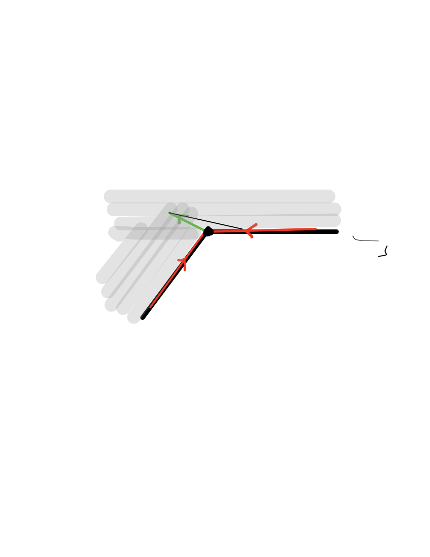
Proof. Geodesics are line segments. We must show that the concatenation of a line segment coming in to the cone point with one exiting the cone point always fails to minimize length. So consider an incoming geodesic ray (in red) and outgoing geodesic segment (green). See figure 1. By rotational symmetry, we can assume that the incoming ray coincides with one of the sector’s bounding rays. Because the two bounding rays are identified to form the cone, the incoming ray actually corresponds to both bounding rays. Since , however we orient the outgoing geodesic segment (green), its angle with one or the other of the two bounding rays is less than . Hence we can “cut the corner” (in black in the figure), skipping the cone point, and shortening the resulting concatenated curve. QED
Lemma 1 establishes the validity of the zero-energy Jacobi-Marchal lemma for the Kepler case, and hence, upon invoking Theorem 2, the Marchal lemma.
Metrics Cones, Generally.
A brief discussion of more general metrics cones is in order.
If is a manifold with Riemannian metric , we form the “metric cone over ” by putting the metric
on , and noting that as the metric on the factor shrinks to zero. Thus, we crunch to a single point, called the cone point. Topologically, crunching is achieved by dividing out by the equivalence relation in which all points are identified with each other. The resulting topological space is the “cone over ”, denoted . The function is then the distance from the cone point, and the ‘spheres” about the cone point are copies of , with the ’s metric scaled by . The case of a cone over the circle corresponds to the case where is a circle of radius . For the theory of general length spaces, and for cones over them, we refer the reader to Burago et al [4].
5. Cones and the zero energy JM metric
The zero energy JM metric is
where is the standard Euclidean metric on . Use spherical coordinates with , , a unit vector. Now assume that is homogeneous of degree . Then we have the “shape potential” , or “normalized potential”
| (4) |
The kinetic energy in spherical coordinates is
where is the standard round metric on the unit sphere . Thus
Solve
with the boundary condition when to get, for 222If then the integral of from to diverges as , this change of variables cannot be made.
and finally
| (5) |
Observe that is the metric for the cone over the sphere of radius . We have shown
Proposition 2.
The zero-energy JM metric for any negative potential which is homogeneous of degree , is given by the expression (5), which is that of a metric conformal to the cone over the sphere of radius with conformal factor the normalized shape potential .
6. The counterexample: Theorem 3.
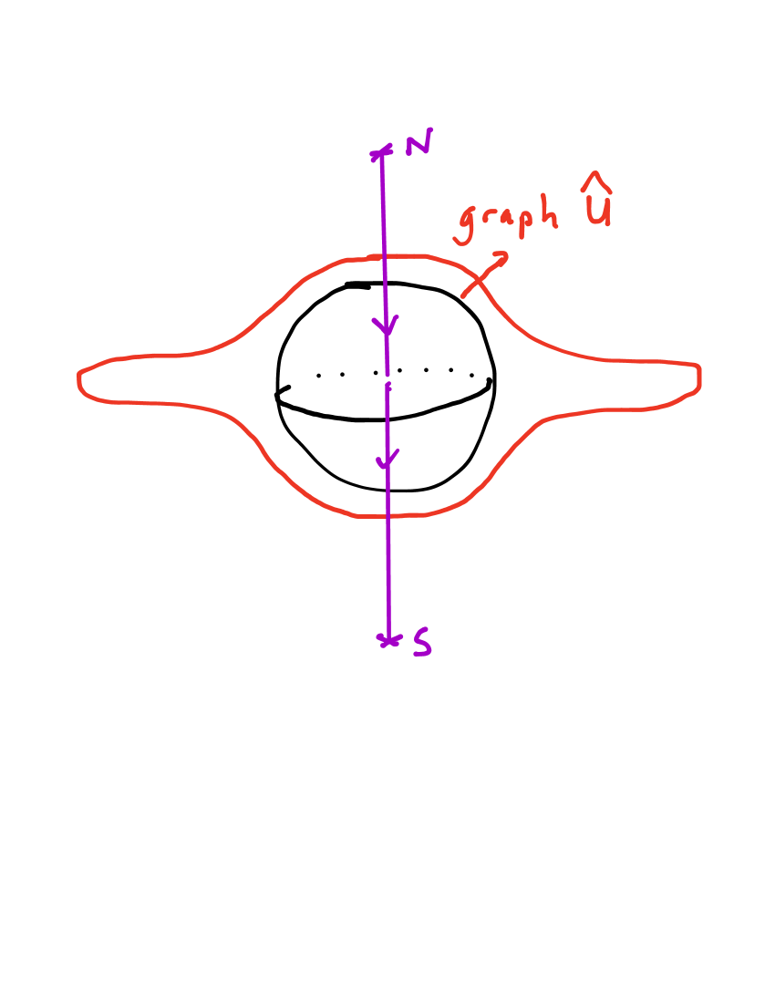
The normal form, eq (5) described in Proposition 2, provides the idea of how to construct a counterexample to Marchal’s lemma, i.e. a potential for which the lemma fails. Design to have absolute minima at the poles N, S of the sphere, while at the same time to be very large in a band surrounding the equator. Look for minimizers from to . Burying straight down through the earth by travelling the Euclidean line segment in joining N to S is a collision path which will be much shorter than travelling along the earth’s surface from N to S since in so doing we must climb the high mountains surrounding the equatorial band. See figure 2. With work this simple idea can be promoted to a proof of Theorem 3.
Let
denote the height coordinate of a point on the sphere so that the North and South poles of the sphere, N and S, are given by while its equator (an -sphere) is defined by . (Here is the last basis vector of our Euclidean configuration space .) For the locus is an equatorial band of thickness . Suppose there are positive constants , and such that satisfies
-
•
(A) achieves its absolute minimum value of at the two poles N and S
-
•
(B) for .
Theorem 4.
Suppose that the normalized potential satisfies (A) and (B) above, that the degree of homogeneity of the potential is with , and that , where . Identify the sphere with the locus as per the representation of eq. (5) and proposition 2. Then the JM-minimizing geodesic connecting the two poles N and S is the Euclidean line segment. In particular, this minimizer passes through collision,showing that the JM Marchal lemma fails for this potential.
6.1. Proof of Theorem 4.
It follows immediately from condition (A) that the minimizing geodesics connecting the sphere to total collision at the origin are the Euclidean line segments obtained by fixing the shape to be one of the two poles and letting vary from to . The length of either segment is , so their concatenation, the line segment described in the statement of the theorem, has length , connects to , and has as an interior collision point. We must show that any curve joining to and avoiding collision has length greater than .
Replace by the piecewise constant function
| (6) |
with corresponding piecewise conical metric
| (7) |
Since and since the two functions agree at the poles we have while . Thus, to prove the theorem it suffices to show that for any curve joining to and not passing through the origin.
Suppose is such a curve. Since joins N to S and along , the spherical part of must cross the equator at some point E. Consider the Euclidean half plane spanned by N and E, and lying on the E side of the line NS. This half-plane is parameterized by and an angle , with which parameterizes the semi-circular longitude N E S. We first show that we may assume that lies inside this half plane. Consider the projection operator
onto the half plane which can be obtained by rotating the spherical part of the point with coordinates until it lies on the longitude NES, while keeping the radial part fixed. Write for a point lying on the equator which is the unit -dimensional Euclidean sphere orthogonal to . Then any point of the sphere can be written
Thus . To see that observe that we can write the spherical element of arclength occuring in eq (5) as and along while . It follows that along the curve the integrand used to compute is less than the same integrand along for and consequently with equality if and only if .
We have reduced our problem to a problem of computing lengths for curves on the half plane relative to the step metric. The metric on the half plane has the form
| (8) |
where we have used polar coordinates , to coordinatize the half-plane. This half plane is cut into three sectors, namely and on which is constant. Now any metric of the form , a positive constant, is locally isometric to the flat Euclidean metric, as we saw earlier in the Kepler section by using the trick of making the substitution which converts the metric to . At this stage it becomes crucial that , as this factor shrinks the opening angle of the half plane to the angle of . Writing
the opening angles of our three sectors are , and . See figure 3
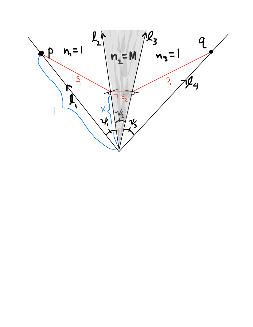
Our step metric on the half-plane consists of a Euclidean metric on each sector, with jump discontinuity as we pass from one sector to the other. Geodesics within each sector are Euclidean lines. The direction of the line suffers a jump discontinuity in crossing from one sector to another according to Snell’s law of optics. The constants and play the role of the index of refraction in Snell’s law.
We now give the final piece of intuition underlying our proof. If then the metric is a uniform Euclidean metric across all sectors and so geodesics are Euclidean straight lines, rather than piecewise linear curves. The metric on the half plane has total opening angle between its bounding rays, rays and , so that the line segment joining N to S does not intersect . Now fix and let increase. The minimizing geodesic bends closer to the vertex, spending less time in the middle region. See the red curve in figure 3. This process is monotonic in M. Eventually, at some critical value the minimizer from N to S disappears into the bounding rays. From then on, for all , the minimizer coincides with . The proof is finished by showing that .
We now fill in the details. Label the bounding rays of the three sectors so that N lies on , lies on and and bound the central sector whose index of refraction is M. Reflection leaves invariant and so is an isometry of the step metric. Since this reflection takes N to S, it follows that any minimizer from N to S is invariant under this reflection. In particular, if the minimizer does enter into the interior of the middle sector, crossing ray a distance from the vertex, then it must leave that middle sector along at the same distance from the vertex. Here we measure relative to the underlying Euclidean metric , which is the metric we multiply by or to get the metric in the various sectors. We have reduced the proof of the proposition to a single variable calculus problem, that of minimizing the step lengths of our one parameter family of “test curves” . Again, see figure 3.
Let us write for the step-length of the test curve labelled by . Then where the are the lengths of the line segments of the test curve in the underlying Euclidean metric and we use the reflectional symmetry to get that . By the law of cosines
while, from trigonometry
Thus
Differentiating with respect to yields
We will show that this derivative is always positive for , provided the condition holds.
Set and observe that . Consequently, the first term of the derivative is . which is always less than or equal to in absolute value. Thus implies that . Now and where we recall the significance of was that for . See item (B) of the conditions 6 above. Now use the inequality which is valid for and . We see that . Thus implies that for . The positivity of this derivative means that the length of these test curves increase monotonically from their absolute minimum value of when , and thus there is no minimizer interior to the sector. QED.
7.
8. Homogeneity. Blow-up. Reduction to zero energy. Theorem 2
Throughout this section we assume that is negative, homogeneous of degree , and smooth away from . We will begin using blow-up to show how the zero energy and nonzero energy JM Marchal lemma are related.
A key step in the usual proof of the Marchal lemma is blow-up: a rescaling argument which reduces the investigation of action minimizers with collision to the case of zero energy action minimizers having a collision. Blow-up is based on the fact that if is homogeneous of degree and if solves the corresponding Newton’s equations then with also solves Newton’s equations. If had energy then has energy .
We proceed to a metric version of blow-up. Consider the dilation map of . Pull back the JM metric by to obtain . Thus
Now a metric and a constant times that metric have the same geodesics, and if a geodesic is a minimizer for one, then it is a minimizer for the other. It follows that if is a minimizing geodesic for joining to then is a minimizing geodesic for joining to . As the curves are uniformly bounded on compact sets , so a subsequence of them converges to a minimizing geodesic for the zero-energy JM metric , one which ends at the cone point. Similarly, if for some there is a minimizing geodesic which ends at the cone point and can be extended past it, then by dilating and taking subsequences, we arrive at extendible minimizing geodesics passing through the cone point.
We have proved
Proposition 3.
Suppose that is homogeneous of degree for , negative, and smooth away from zero. Then the JM-Marchal lemma holds for at energy if and only if it holds for at energy .
8.1. Proof of theorem 2
[due to Andrea Venturelli] We proceed by proving the contrapositive. Suppose that the Marchal lemma for total collisions 333i.e. the only collision available under our hypothesis, fails for a particular potential of homogeneity . We will show that the JM-Marchall lemma also fails for this potential. The failure of the Marchal lemma for total collisions means that there exists a curve which has an internal total collision and is a fixed time minimizer between its endpoints. Translate time so the total collision occurs at time . By a standard argument ([14], [5], section 3.2.1), the rescaled family , with , converges as , to a curve
which is the concatenation of two parabolic homothetic solutions, defined for and for . (The convergence is uniform on bounded intervals containing .) Moreover, is a global fixed time minimzer: that is, for each pair of times the segment is a fixed time action minimizers between its endpoints and . If we knew the concatenation was a free time minimizer, rather than just a fixed-time minimizer, between all pairs of its points then we would be done, by Proposition 1 . But we don’t know that yet.
We now argue by contradiction. Suppose that the concatenation is not a global free time minimizer. Then there must exist two points along , one before collision, one after, for which there is curve joining these two points and having smaller action. Write the points as and , for . Then the curve satisfies and . Set . For large positive consider the concatentation
with two of the curves in this concatenation requiring a time shift in their parameterizations to guarantee that they take off when the previous curve ends. The action of is
where
However, the the interval parameterizing is not but rather whose length is . To finish off the proof we must reparameterize so as to be parameterized an interval of length with the penalty of possibly increasing the action, but not enough to swamp the . We will estimate that this this increase due to reparameterization is , so that taking sufficiently large will complete the proof.
The ratio of the two intervals of parameterization is
So set
yielding a reparameterization of by an interval of length . If the action then one computes that where . But where , and . Thus which is less than and gives us our contradiction.
QED.
9. Comparison with the Work of Barutello et al
In a tour-de-force of variational and dynamical analysis Barutello, Terracini and Verzini [2], [3] have thoroughly investigated a class of problems very similar to ours. They consider negatively homogeneous potentials for which is positive, sufficiently smooth and takes on its minimum at precisely two distinct points . The authors also assume both minima are nondegenerate. Denote the set of all such normalized potentials on the sphere by . Then they coordinatize the space of all their potentials by and where . For each such potential they ask “does the free time action minimizer joining to pass through total collision ()?” If the answer is ‘yes’ they call the potential labelled by an ‘IN’ potential, and otherwise they call that potential an “OUT” potential, in this manner decomposing the space of all potentials into two disjoint sets. Their main result is that there is a continuous function such that if then is an IN potential, while if then this potential is an OUT potential. (The function is denoted in their paper.)
From the perspective of Barutello et al then, our theorem 4 asserts that if then the potential is of “IN” type. Doing some algebra, we see that this inequality holds if and only if , which logically implies the estimate .
Barutello et al have a quite pleasing characterization of the value as a “phase transition” in variational behavioir. To begin the characterization they need to define wha it means to be a “free-time Morse minimizer”. In our definition above of “ free-time minimizer”, the minimizer joined two fixed points , and had domain a closed bounded interval . (Barutello, Terracini and Verzini call this type of minimizer a “Bolza minimizers”.) If the domain of is the entire line and if its restriction to any compact sub-interval is a free-time minimizer in our sense, then is called a free-time Morse minimizer. (In [9] this type of minimizer is called a “‘global free time minimizer”.) The value is the unique value of the homogeneity for which a free-time Morse minimizer exists. To see what happens, choose endpoints on the ray and on the ray with and join and by a free-time minimizer . Now let . For the curves disappears off to infinity. For the curves converge to the collision-ejection concatenation of two parabolic minimizers, which is the case where the Marchal lemma fails. Exactly at we get a nice convergence of to a free-time Morse minimizer. This limit curve is a parabolic non-colliision solution to Newton’s equation connecting to .
To compare our set-up in Theorem 4 with theirs, observe that we have specialized to the case , but have relaxed the condition that these two points are the only two absolute minima, thus allowing for the minimum level set to be a continuum, as it will be for any potential with a continuous symmetry group.
10. Back to Why
Armed with the knowledge of how the Marchal lemma can fail, let us ammend and return to our original question: “Why does Marchal’s lemma hold for the power law potentials?” I will not give a full metric-inspired proof of the lemma, but rather a sketch of plausible geometric mechanisms behind the lemma.
The heart of the idea is contained in section 4. I would like to answer “Marchal’s lemma holds due to the conical nature of the JM metric near collisions.”. This answer is incomplete for two reasons. First, at total collision the metric is not actually conical, but rather is conformal to a conical metric (Proposition 2), and we have seen that certain conformal factors can make the lemma fail (Theorem 4). The second reason is that there is no longer a single total collision point, but rather an entire collision locus and the nature of the metric depends on which stratum of this locus we are approaching.
Before describing this plausibility mechanism, suppose that I could show that Theorem 2 held for the power law potentials, which is to say that for these potentials the zero energy JM Marchal lemma implied the standard Marchal lemma. Then it would be legitimate to focus my attention on establishing the zero energy JM Marchal lemma.
The zero energy JM-metric is a Riemannian metric defined away from collisions and so yields a metric distance function on where denotes the collision locus. When and any point on the collision locus can be reached by any point on the non-collision locus by a path of finite JM length. Moreover all paths to infinity have infinite JM length. Thus, the metric completion of with this distance function is all of . The assertion of Marchal’s lemma now becomes any geodesic for this metric which ends in collision is inextendible. See Appendix A for the notion of geodesics on metric spaces, and definition 6 there for that of a geodesics being inextendible.
To this end, let be any minimizing geodesic ending in collision. Then any subsegment of is also a minimizing geodesic. Moreover cannot lie on the collision locus for if it did its length would be infinite. So there is a non-collision point along . Let be the first collision time greater than along , so that while is collision-free. The aim is to show that is inextendible.
If is a total collision point then we can use the normal form (Prop. 2) for the metric. Let denote the central configurations, which is to say, the critical points of on the unit sphere , . For each , the ray , reparameterized, and traversed backwards, is a geodesic ending in total collision. These rays are the usual homothetic parabolic central configuration solutions in the N-body problem. Then is asymptotic to one of these central configuration geodesics as . Any geodesic extension of past would be asympotic to some other central configuration geodesic as . Using the metric dilations of the cone, we can expand to the limiting case where both the incoming and outgoing geodesics are central configuration rays.
We are now in a situation similar to that investigated in the proof of Theorem 4. There we proved the geodesic could be extended. We want to prove our initial geodesic cannot be extended. Any extension would correspond to concatenating the incoming geodesic with an outgoing one, itself asymptotic to another outgoing central configuration ray. So we reduce, as in the usual proof of Marchal, to the case of two central configuration rays concatentated at total collision. The idea for showing that this concatenation cannot be a minimizer is to first establish that between any two central configurations there is a low mountain pass. In other words, given any two central configurations, there is a path on the sphere which joins them and along which the maximum of is fairly small, while the path’s length is not so long. We will call such a path a “mountain pass path”. In the three-body case, imagine the incoming and outgoing rays to be the positively and negatively oriented Lagrange triangles – the North and South pole of the shape sphere – while the mountain pass curve cuts through the collinear equator at an Euler point. The alleged result then, would be that if we work on the cone over this mountain pass path, we can connect the two central configurations without ever touching total collision, or indeed any collision, since this mountain pass path will be collision-free.
What do we do if is not a total collision? My idea here is more vague. I propose copying the transformations around cluster expansions as used in the inductive arguments of one or the other of the standard proofs of Marchal’s lemma ([7], [14]) and arguing that near collision the metric approximately “splits” into a metric governing motion normal to the stratum (“cluster type”) of the collision point, and a metric tangential to the stratum, the latter being times a blowing up factor where is distance from the stratum. Project geodesics onto the normal part of the metric. Hope that the structure of the metric along this normal part is such that the previous (and incomplete) total collision argument can be used.
This sketch of a proof is conjectural, but the picture it gives affords me some satisfaction. Morevoer, the argument can legitemately be run backwards, since we know that Marchal implies the zero energy JM-Marchal lemma (Theorem 1), thus giving some information regarding the geometry around mountain passes associated to the power law on the sphere.
Appendix A Appendix. Metric Geometry and Collision Mechanics.
We recall a few concepts from metric geometry and relate them to the JM metric. A “length space” is a metric space such that the distance between any two points is equal to infimum of the lengths of the paths joining the two points. A minimizing geodesic between p and q is a curve joining them which realizes this infimum: its length equals . Any minimizing geodesic can be parameterized by arclength, in which case for all in the domain of .
What then, is a geodesic in ? Let be a sub-interval, possibly infinite in one or both directions. A ‘geodesic” in is a curve which is parameterized by arclength and such that about any point in the interior of the time interval there is an such that the restriction of to is a minimizing geodesic between its endpoints. (If is an endpoint of we make a similar minimality requirement, using intervals having one endpoint instead.)
Definition 6.
A geodesic is inextendible beyond if it admits no extension which is a geodesic.
Example 2.
If is the upper half plane with its usual Euclidean metric, then the geodesics are line segments lying in . A geodesic is inextendible if it begins in the interior of the upper half plane and ends on the boundary.
The JM length functional defines a metric geometry away from the Hill boundary and collisions, which is to say, on the domain of . The distance between two points of the domain is the infimum of the lengths of all paths lying in the domain and joining to .
However, this distance will typically not complete be complete. We can try to complete it by adding points of the closure of the domain, which is to say the Hill boundary and the collision locus , together, possibly, with some points at infinity. Now if and lie in the same path component of the Hill boundary we can travel from p to q by a path lying in the boundary in which case . So we have a choice: accept that the extended metric is not a true metric, but rather only a semi-metric, or collapse each boundary component of the Hill boundary to a single point.
Suppose, for simplicity, that our potential is negative so that the Hill boundary is empty when the energy is zero or negative. Then we can ignore problems with the Hill boundary. Suppose also that the collision locus does not separate . Then the distance is well-defined and finite for any two non-collision points. Let us also suppose that any path tending to infinity (meaning along which is unbounded) has infinite length. Then the metric completion of is obtained by adding back in all those collision points for which there is a finite length path which ends in them.
For example, with the power law potentials, this completion strategy works beautifully when . When and the energy is zero, then all paths to collision have infiniite length and so is already complete. (See [10].) When any path ending in collision continues to have infinite length, but now there are finite length radial paths extending out to infiniity , so that points (only one?) at infinity must be added to obtain the metric completion of .
The general case of negative potentials having homogeneity which are not power law potentials, and which have collision points besides the origin, could yield JM metrics with quite complicated metric completion, depending crucially on how the potential blows up along “spherical directions” as points of the collision locus are approached. It would be of interest to encounter important or useful examples of such potentials.
Appendix B Appendix. Metric Geometry of Hill boundary
The Jacobi-Maupertuis metric degenerates to zero at the Hill boundary . Newtonian solutions with energy reflect off the Hill boundary, retracing their path. At the instant of reflection the kinetic energy is zero and hence the velocity is zero. Such solutions are called “brake solutions” with the brake instant.
To establish that this retracing occurs observe that whenever is a solution to Newton’s equations, so is . Now both and have that same initial conditions, namely , at . It follows from uniqueness that the two solutions are equal: , which is the assertion of retracing. Geodesics cannot retrace their own paths. Brake solutions, insofar as they can be considered to be JM geodesics, are inextendible past the brake moment.
Acknowledgements
I would like to thank Andrea Venturelli, Mark Levi, Alain Albouy, Alain Chenciner, Vivina Barutello, Rick Moeckel, and Hector Sanchez for helpful conversations. I thankfully acknowledges support by the NSF, grant DMS-20030177.
Appendix C
References
- [1] R. Abraham and J. E. Marsden, Foundations of Mechanics, 2nd ed. Benjamin/Cummings, 1978.
- [2] V. Barutello, S. Terracini, and G. Verzini, Entire minimal parabolic trajectories: the planar anisotropic Kepler problem, Arch. Ration. Mech. Anal., 207(2):583-609, (2013).
- [3] V. Barutello, S. Terracini, and G. Verzini,Entire parabolic trajectories as minimal phase transitions, Calc. Var. Partial Differential Equations, vol. 49, no. 1-2, 391-429, (2014).
- [4] D. Burago, Y. Burago, S. Ivanov, A course in metric geometry. Graduate Studies in Mathematics, 33. American Mathematical Society, Providence, RI, 2001.
- [5] A. Chenciner, Action minimizing solutions of the n-body problem: from homology to symmetry, Proceedings of the Int. Congress of Mathematicians, (ICM 2002), Peking, vol. III, pp. 279-294, (2002).
- [6] A. Chenciner and R. Montgomery, A remarkable periodic solution of the three-body problem in the case of equal masses, with Alain Chenciner, Annals of Mathematics, 152, 881-901 (2000).
- [7] D. Ferrario and S. Terracini, On the existence of collisionless equivariant minimizers for the classical n-body problem, Invent. Math. vol. 155, no. 2, 305-362, (2004),
- [8] W. Gordon, A minimizing property of Keplerian orbits, Am J. Math., v. 99, no. 5, 961-971, (1977).
- [9] R. Moeckel, R. Montgomery, and H. Sanchez, Free time minimizers for the planar three-body problem , Celestial Mechanics and Dynamical Astronomy, vol. 130, no. 3, article 28 (on-line version), ( 2018).
- [10] R. Montgomery, Fitting hyperbolic pants to a three-body problem, Ergodic Theory Dynam. Systems, v. 25, no. 3, 921–947, (2005).
- [11] R. Montgomery, Who’s afraid of the Hill boundary? -conjugate loci clustering at the boundary, SIGMA vol. 10, pp 101, (2014)
- [12] C. Marchal How the method of minimization of action avoids singularities, Celestial Mechanics and Dynamical Astronomy, vol. 83, no. 1, pp. 325–353, (2002). DOI : 10.1023/A:1020128408706
- [13] H. Seifert, Periodische Bewegungen Mechanischer Systeme, Math. Z. , vol. 51, (1948). (an English translation is available at: http://people.ucsc.edu/~rmont/papers/list.html under the year 2006.)
- [14] A. Venturelli Une caractérisation variationnelle des solutions de Lagrange du problème plan des trois corps, C.R. Acad. Sci. Paris, t. 332, Série I, p. 641-644, (2001).
- [15] A. Wintner, The Analytical Foundations of Celestial Mechanics, Princeton Mathematical Series, v. 5. Princeton University Press, Princeton, N. J., 1941