3D Fluid Flow Estimation with Integrated Particle Reconstruction

Abstract

The standard approach to densely reconstruct the motion in a volume of fluid is to inject high-contrast tracer particles and record their motion with multiple high-speed cameras. Almost all existing work processes the acquired multi-view video in two separate steps, utilizing either a pure Eulerian or pure Lagrangian approach. Eulerian methods perform a voxel-based reconstruction of particles per time step, followed by 3D motion estimation, with some form of dense matching between the precomputed voxel grids from different time steps. In this sequential procedure, the first step cannot use temporal consistency considerations to support the reconstruction, while the second step has no access to the original, high-resolution image data. Alternatively, Lagrangian methods reconstruct an explicit, sparse set of particles and track the individual particles over time. Physical constraints can only be incorporated in a post-processing step when interpolating the particle tracks to a dense motion field. We show, for the first time, how to jointly reconstruct both the individual tracer particles and a dense 3D fluid motion field from the image data, using an integrated energy minimization. Our hybrid Lagrangian/Eulerian model reconstructs individual particles, and at the same time recovers a dense 3D motion field in the entire domain. Making particles explicit greatly reduces the memory consumption and allows one to use the high-resolution input images for matching. Whereas the dense motion field makes it possible to include physical a-priori constraints and account for the incompressibility and viscosity of the fluid. The method exhibits greatly ($\approx\!70\%$) improved results over our recently published baseline with two separate steps for 3D reconstruction and motion estimation. Our results with only two time steps are comparable to those of state-of-the-art tracking-based methods that require much longer sequences.

1 Introduction

Motion estimation of fluids is a challenging task in experimental fluid mechanics with important applications in research and industry: Observations of fluid motion and fluid-structure interaction form the basis of experimental fluid dynamics. Measuring and understanding flow and turbulence patterns is important for aero- and hydrodynamics in the automotive, aeronautic and ship-building industries, e.g. to design efficient shapes and to test the elasticity of components. Biological sciences are another application field, e.g., behavioral studies about aquatic organisms that live in flowing water, or the analysis of the flight dynamics of birds and insects (Michalec et al.,, 2015; Wu et al.,, 2009).

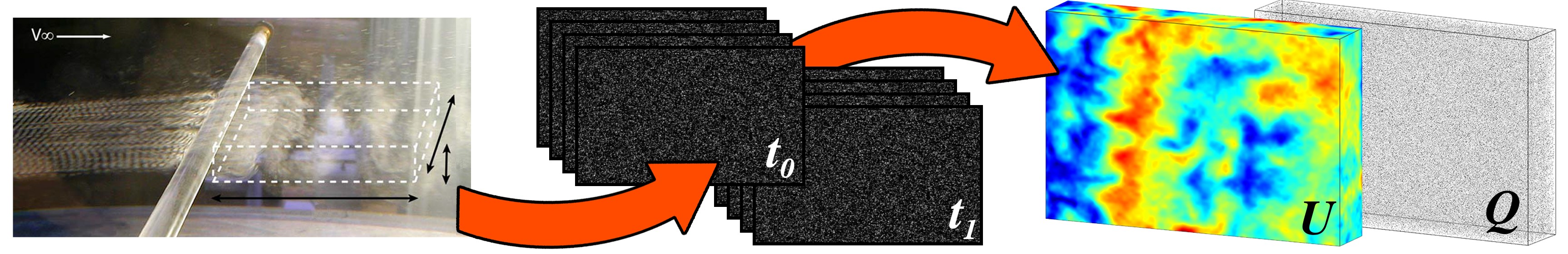
Figure 1: From 2D images of a fluid injected with tracer particles, recorded at two consecutive time steps, we jointly reconstruct the particles $\mathcal{Q}$ and a dense 3D motion field $\mathcal{U}$. The example shows the experimental setup of Michaelis et al., (2006).

To capture fluid motion, one common approach is to inject tracer particles into the fluid, which densely cover the illuminated area of interest, and to record them with one or multiple high-speed cameras. From this idea two strategies have evolved in experimental fluid mechanics: particle image velocimetry (PIV) and particle tracking velocimetry (PTV) (Adrian and Westerweel,, 2011; Raffel et al.,, 2018). PIV outputs a dense velocity field (Eulerian view), while PTV computes a flow vector at each particle location (Lagrangian view).

In the standard 2D-PIV setup, a thin slice of the measurement area is illuminated by a laser scanner, allowing only for 2D in-plane motion estimation. Motion vectors are recovered on a dense regular grid by correspondence matching of local support windows (in PIV terminology “interrogation windows”). In contrast, particle tracking velocimetry (PTV) employs a Lagrangian view of the problem by tracking individual particles over multiple time steps and effectively describing the motion of the fluid only on those sparse locations. Since individual particles have to be identified, the maximum allowed seeding density is usually lower than for PIV measurements, where particle constellations are matched instead.

In the 3D setup, a measurement volume is illuminated with a thick laser slice and observed by synchronized cameras from multiple viewpoints. We illustrate the basic setup in Fig. 1: 3D Particle locations and a dense motion field are recovered from a set of input images from two consecutive time steps. There is a trade-off regarding the seeding density of the particles: A higher density delivers an increased effective spatial resolution, but also raises the ambiguity of the matching.

Both Eulerian and Lagrangian approches have been proposed to tackle the problem in 3D (c.f. Maas et al., (1993); Elsinga et al., (2006); Champagnat et al., (2011); Discetti and Astarita, (2012); Cheminet et al., (2014); Lasinger et al., (2017); Schanz et al., (2016)), coming with their individual architectural problems. Eulerian approaches perform 3D reconstruction and motion estimation in two sequential steps and require large voxel volumes to represent the high-frequency particle data. Lagrangian approaches, on the other hand, require tracking over multiple time steps to resolve ambiguities in the triangulation, and cannot directly incorporate physical constraints.

In this work we propose a joint energy model for the reconstruction of the particles and the 3D motion field from two time steps, so as to capture the inherent mutual dependencies. The model uses the full information – all available images from both time steps at full resolution – to solve the problem. We opt for a hybrid Lagrangian/Eulerian formulation: particles are modeled individually, while the motion field is represented on a dense grid. Recovering explicit particle locations and intensities sidesteps the costly 3D parameterization of voxel occupancy, as well as the use of a large matching window. Instead, it directly compares evidence for single particles in the images, yielding significantly higher accuracy.

To represent the motion field, we opt for a trilinear finite element basis. Modeling the 3D motion densely allows us to incorporate physical priors that account for incompressibility and viscosity of the observed fluid, similar to our previous work (Lasinger et al.,, 2017). This can be done efficiently, at a much lower voxel resolution than would be required for particle reconstruction, due to the smoothness of the 3D motion field (Cheminet et al.,, 2014; Lasinger et al.,, 2017).

We model our problem in a variational setting. To better resolve particle ambiguities, we add a prior to our energy that encourages sparsity. In order to overcome weak minima of the non-convex energy, we include a proposal generation step that detects putative particles in the residual images, and alternates with the energy minimization. For the optimization itself, we can rely on the very efficient inertial Proximal Alternating Linearized Minimization (iPALM) (Bolte et al.,, 2014; Pock and Sabach,, 2016). It is guaranteed to converge to a stationary point of the energy and has a low memory footprint, so that we can reconstruct large volumes.

Compared to the baselines of Elsinga et al., (2006) and our own previous work (Lasinger et al.,, 2017), which both address the problem sequentially with two independent steps, we achieve particle reconstructions with higher precision and recall, at all tested particle densities; as well as greatly improved motion estimates. The estimated fluid flow visually appears on par with state-of-the-art techniques like Schanz et al., (2016), which use tracking over multiple time steps and highly engineered post-processing (Schneiders and Scarano,, 2016; Gesemann et al.,, 2016).

The present paper is based on the preliminary version (Lasinger et al.,, 2019). We have extended the original approach by integrating also the polynomial camera model by Soloff et al., (1997). This model compensates for refractions at air-glass and glass-water transitions and thus allows for experiments with liquids, such as water. Furthermore, we have added additional experiments and visualizations for setups both in water and air.

2 Related Work

We focus here on 3D-PIV and PTV approaches, and refer to Adrian and Westerweel, (2011) or Raffel et al., (2018) for an exhaustive review of 2D techniques. The first method to operate on 3D fluid volumes was the Lagrangian 3D-PTV method (Maas et al.,, 1993), where individual particles are detected in different views, triangulated and tracked over time. Yet, as the seeding density increases the particles quickly start to overlap in the images, leading to ambiguities. Therefore, 3D-PTV is only recommended for densities $<0.005$ ppp (particles per pixel). To handle higher seeding densities, Elsinga et al., (2006) introduced the Eulerian Tomo-PIV method. They first employ a tomographic reconstruction (e.g. MART) (Atkinson and Soria,, 2009) per time step, to obtain a 3D voxel space of occupancy probabilities. Cross-correlation with large local 3D windows ($\geq 35^{3}$) (Champagnat et al.,, 2011; Discetti and Astarita,, 2012; Cheminet et al.,, 2014) then yields the flow. Effectively, this amounts to matching particle constellations, assuming constant flow in large windows, which smooths the output to low effective resolution. Recently, a new Lagrangian particle tracking method Shake-the-Box (StB) was introduced (Schanz et al.,, 2016). It builds on the idea of iterative particle reconstruction (IPR) (Wieneke,, 2013), where triangulation is performed iteratively, with a local position and intensity refinement after every triangulation step. In subsequent time steps, particle locations are predicted from trajectory information from previous time steps, and refined by small perturbations in all directions (”shaking”) to find the location with the lowest reprojection error.

None of the above methods accounts for the physics of (incompressible) fluids during reconstruction. In StB (Schanz et al.,, 2016), a post-process interpolates sparse tracks to a regular grid. At that step, but not during reconstruction, physical constraints can be included (Schneiders and Scarano,, 2016; Gesemann et al.,, 2016). Variational approaches that impose physically consistent regularizers were first proposed for the 2D PIV setup. Ruhnau and Schnörr, (2007) presented an optical flow-based approach that incorporates physical priors using the Stokes equations. In (Ruhnau et al.,, 2006) this idea was further extended to the full Navier-Stokes equations. With the help of the vorticity transport equation they obtain a spatio-temporal regularization that can model turbulent fluids. A drawback of the method is that the vorticity is usually not known beforehand, thus it has to be initialized with $\omega=0$, and observations from several time steps are needed for the estimation to converge ($\approx 5$ in their experiments).

In our earlier work (Lasinger et al.,, 2017) we have proposed a 3D variational approach that combines TomoPIV with variational 3D flow estimation. We account for physical constraints with a regularizer derived from the stationary Stokes equations, similar to Ruhnau and Schnörr, (2007). However, the voxel-based data term requires a huge, high-resolution intensity volume, and a local window of $11^{3}$ voxels for matching, which lowers spatial resolution, albeit less than earlier local matching. To overcome the memory bottleneck, we have further proposed a sparse particle representation (Lasinger et al.,, 2018). 3D particle reconstruction and motion estimation are still performed sequentially. Then local particle constellations are encoded in a descriptor and matched. The need to rely on spatial context limits the spatial resolution of the resulting flow field. Gregson et al., (2014) proposed an approach similar to Lasinger et al., (2017) for dye-injected two-media fluids. Their aim are visually pleasing, rather than physically correct results, computed for relatively small volumes ($\approx\!100^{3}$ voxels). We note that dye leads to data that is very different from tracer particles, i.e., it produces structures along the transition surface between water and dye that can be matched well across time, but does not afford data evidence in large parts of the volume. Dalitz et al., (2017) use compressive sensing to jointly recover the location and motion of a sparse, time-varying signal with a mathematical recovery guarantee. Results are only shown for small grids ($256^{3}$), and the physics of fluids is not considered. Barbu et al., (2013) introduce a joint approach for 3D reconstruction and flow estimation, however, without considering physical properties of the problem. Their purely Eulerian, voxel-based setup limits the method to small volume sizes, i.e., the method is only evaluated on a $61\times 61\times 31$ grid and a rather low seeding density of 0.02 ppp. Xiong et al., (2017) propose a joint formulation for their single-camera PIV setup. The volume is illuminated by rainbow-colored light planes that encode depth information. This permits the use of only a single camera with the drawback of lower depth accuracy and limited particle seeding density. Voxel occupancy probabilities are recovered on a 3D grid. To handle the ill-conditioned problem from a single camera, constraints on particle sparsity and motion consistency (including physical constraints) are incorporated in the optimization. The method operates on a “thin” maximum volume of $512\times 270\times 20$. The single-camera setup does not allow a direct comparison with standard 3D PIV/PTV, but can certainly not compete in terms of depth resolution. In contrast, by separating the representation of particles and motion field, our hybrid Lagrangian/Eulerian approach allows for sub-pixel accurate particle reconstruction and large fluid volumes. Finally, Ruhnau et al., (2005) propose a hybrid discrete particle and continuous variational motion estimation approach. Particle reconstruction and motion estimation are performed sequentially, and without physically plausible regularization of the flow.

Volumetric fluid flow is also related to variational scene-flow estimation, especially methods that parameterize the scene in 3D space (Basha et al.,, 2010; Vogel et al.,, 2011). Like those, we search for the geometry and motion of a dynamic scene and exploit multiple views, yet our goal is a dense reconstruction in a given volume, rather than a pixel-wise motion field. Scene flow has undergone an evolution similar to the one for 3D fluid flow. Early methods started with a fixed, precomputed geometry estimate (Wedel et al.,, 2011; Rabe et al.,, 2010), with a notable exception (Huguet and Devernay,, 2007). Later work moved to a joint reconstruction of geometry and motion (Basha et al.,, 2010; Valgaerts et al.,, 2010; Vogel et al.,, 2011). Likewise, Elsinga et al., (2006) and Lasinger et al., (2017) precompute the 3D tracer particles before estimating their motion. The method described in the present paper is, to our knowledge, the first multi-camera PIV scheme that jointly determines the explicit locations of all particles and the physically constrained motion of the fluid.

Several scene flow methods (Vogel et al.,, 2013, 2015; Menze and Geiger,, 2015) overcome the large state space by sampling geometry and motion proposals, and perform discrete optimization over those samples. In a similar spirit, we employ IPR to generate discrete particle proposals, but then combine them with a continuous, variational optimization scheme. We note that discrete labeling does not suit our task: The volumetric setting would require an excessive number of labels (3D vectors), and enormous amounts of memory. And it does not lend itself to sub-voxel accurate inference.

The discretization of our motion field is based on the finite element method (FEM) (Courant,, 1943; Reddy,, 1993; Brezzi and Fortin,, 1991). FEM has been applied to variational problems in computer vision, including 2D PIV (Ruhnau et al.,, 2006; Ruhnau and Schnörr,, 2007) and semantic 3D reconstruction (Richard et al.,, 2017).

3 Method

To set the scene, we restate the goal of our method: densely predict the 3D flow field in a fluid seeded with tracer particles, from multiple 2D views acquired at two adjacent time steps.

We aim to do this in a direct, integrated fashion. The joint particle reconstruction and motion estimation is cast into a hybrid Lagrangian/Eulerian model, where we recover individual particles and keep track of their position and appearance, but reconstruct a continuous 3D motion field in the entire domain. A dense sampling of the motion field makes it technically and numerically easier to adhere to physical constraints like incompressibility. In contrast, modeling particles explicitly takes advantage of the low particle density in PIV data. Practical densities are around $0.1$ particles per pixel (ppp) in the images. Depending on the desired voxel resolution, this corresponds to 10-1000 times lower volumetric density. Our complete pipeline is depicted in Fig. 2. It alternates between generating particle proposals (Sec. 3.2) based on the current residual images (starting from the raw input images), and energy minimization to update all particles and motion vectors (Sec. 3.3). The corresponding variational energy function is described in Sec. 3.1. In the process, particle locations and flow estimates are progressively refined and provide a better initialization for further particle proposals.

Particle triangulation is highly ambiguous, so the proposal generator will inevitably introduce many spurious “ghost” particles (Fig. 3). A sparsity term in the energy reduces the influence of low intensity particles that usually correspond to such ghosts, while true particles, given the preliminary flow estimate, receive additional support from the data of the second time step. In later iterations, already reconstructed particles vanish in the residual images. This allows for a refined localization of remaining particles, as particle overlaps are resolved.

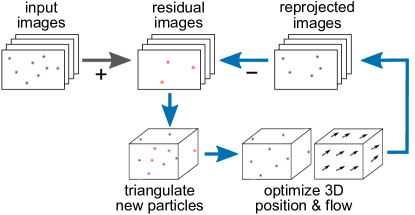
Figure 2: Particle position and flow estimation pipeline. We alternate between joint optimization of 3D particle positions and dense flow vectors, and adding new candidate particles by triangulation from the residual images.

Notation and Preliminaries.

The scene is observed by $K$ calibrated cameras $\mathcal{K}_{k},k=1,\ldots,K$, recording the images $\mathcal{I}^{t}_{k}$ at time $t$. Parameterizing the scene with 3D entities obviates the need for image rectification. Fluid experiments typically need sophisticated models to deal with refraction (air-glass and glass-water), or an optical transfer function derived from volume self-calibration (Wieneke,, 2008; Schanz et al.,, 2012). We keep the formulation general with a generic projection operator $\Pi_{k}$ per camera. For convenience, we include two important cases of $\Pi_{k}$, the pinhole camera model (e.g. for measurements in air) and a polynomial camera model designed for multi-media experiments (air-glass-water) (Soloff et al.,, 1997).

The dependency on time is denoted via superscript $t_{0},t_{1}$, and omitted when possible. We denote the set of particles $\mathcal{Q}:=\{(p_{i},c_{i})\}_{i=1}^{Q}$, composed of a set of intensities $\mathcal{C}:=\{c_{i}\}_{i=1}^{Q}$, $c_{i}\in\mathbb{R}^{+}_{0}$ and positions $\mathcal{P}:=\{p_{i}\}_{i=1}^{Q}$, where each $p_{i}\in\mathbb{R}^{3}$ is located in the rectangular domain $\Omega\subset\mathbb{R}^{3}$. The 3D motion field at position $x\in\Omega$, between times $t_{0}$ and $t_{1}$, is $u(x,\mathcal{U})$. The set $\mathcal{U}$ contains motion vectors $u\in\mathbb{R}^{3}$ located at a finite set of positions $y\in\mathcal{Y}\subset\Omega$. If we let these locations coincide with the particle positions, we would arrive at a fully Lagrangian design, also referred to as smoothed particle hydrodynamics (Monaghan,, 2005; Adams et al.,, 2007). In this work, we prefer a fixed set $\mathcal{Y}$ and represent the functional $u(x,\mathcal{U})$ by trilinear interpolation, i.e. we opt for an Eulerian description of the motion. Our model is, thus, similar to the so-called particle in cell design (Zhu and Bridson,, 2005). Without loss of generality, we assume $\mathcal{Y}\subset\Omega\cap\mathbb{Z}^{3}$, i.e., we set up a regular grid of vertices $\mathbf{i}\in\mathcal{Y}$ of size $N\times M\times L$, which induce a voxel covering $V(\Omega)$ of size $N-1\times M-1\times L-1$ of the whole domain. We use a trilinear FEM discretization, i.e., each grid vertex $\mathbf{i}=(\mathbf{i}_{1},\mathbf{i}_{2},\mathbf{i}_{3})^{\!\mathsf{T}}$ is associated with a trilinear basis function:

$$\begin{split}\mathbf{b}_{\mathbf{i}}(x):=\prod_{l=1}^{3}\max(0,1-|&x_{l}-\mathbf{i}_{l}|),\\[-8.61108pt] &\textrm{ for }x=(x_{1},x_{2},x_{3})^{\!\mathsf{T}}.\end{split}$$ (1)

The elements $u_{\mathbf{i}}\in\mathcal{U}$ now represent the coefficients of our motion field function $u(x,\mathcal{U}),x\in\Omega$ that is given by:

$$\begin{split}u(x,\mathcal{U})=&\big{(}u_{1}(x,\mathcal{U}),u_{2}(x,\mathcal{U}),u_{3}(x,\mathcal{U})\big{)}^{\!\mathsf{T}}\\[4.30554pt] &\textrm{with}\ u_{l}(x,\mathcal{U})=\sum_{\mathbf{i}\in\mathcal{Y}}\mathbf{b}_{\mathbf{i}}(x)u_{\mathbf{i},l}\;,\ l=\textrm{1,2,3}.\end{split}$$ (2)

Finally, in our energy formulation we make use of the indicator function $\delta_{\mathcal{C}}$ defined for a (not necessarily convex) set $\mathcal{C}$ (Boyd and Vandenberghe,, 2004; Bertsekas,, 1999):

$$\delta_{\mathcal{C}}(x):=\left\{\begin{array}[]{cc}0&\quad\textrm{ if }x\in\mathcal{C}\\ \infty&\quad\textrm{else}\end{array}\right..$$ (3)

3.1 Energy Model

With the definitions above, we can write the energy

$$E(\mathcal{P},\mathcal{C},\mathcal{U}):=\frac{1}{2}E_{\textrm{D}}(\mathcal{P},\mathcal{C},\mathcal{U})+\frac{\lambda}{2}E_{\textrm{S}}(\mathcal{U})+\mu E_{\textrm{Sp}}(\mathcal{C}),$$ (4)

with a data term $E_{\textrm{D}}$, a smoothness term $E_{\textrm{S}}$ operating on the motion field, and a sparsity prior $E_{\textrm{Sp}}$ operating on the intensities of the particles.

3.1.1 Data Term

To compute the data term, the images of all cameras at both time steps are predicted from the particles’ positions and intensities, and the 3D motion field. $E_{\textrm{D}}$ penalizes deviations between predicted and observed images:

$$\begin{split}&E_{D}(\mathcal{P},\mathcal{C},\mathcal{U}):=\\ &\;\frac{1}{K}\!\sum_{k=1}^{K}\!\int_{\Gamma_{k}}\!\!\!\big{|}\mathcal{I}^{t_{0}}_{k}(x)\!-\!\!\sum_{i=1}^{P}\!\Pi_{k}(c_{i}\!\cdot\!\mathcal{N}(p_{i},\sigma)(x)\!)\big{|}_{2}^{2}\mathrm{d}x\ +\\ &\;\frac{1}{K}\!\sum_{k=1}^{K}\!\int_{\Gamma_{k}}\!\!\!\big{|}\mathcal{I}^{t_{1}}_{k}(x)\!-\!\!\sum_{i=1}^{P}\!\Pi_{k}(c_{i}\!\cdot\!\mathcal{N}(p_{i}\!+\!u(p_{i},\mathcal{U}),\sigma)(x)\!)\big{|}_{2}^{2}\mathrm{d}x.\end{split}$$ (5)

Following an additive (in terms of particles) image formation model, we integrate over the image plane $\Gamma_{k}$ of camera $k$. Individual particles $(p,c)\in\mathcal{Q}$ are represented by Gaussian blobs with variance $\sigma^{2}$. Particles do not exhibit strong shape or material variations. Their distance to the light source does influence the observed intensity. But since it changes smoothly and the cameras record with high frame-rate, assuming constant intensity is a valid approximation for our two-frame model.

In practical setups, the depth range of the volume $\Omega$ is small compared to the distance from the cameras. Therefore, the projection is close to orthographic, such that particles undergo almost no perspective distortion, and their image projections are 2D Gaussian blobs. In that regime, and omitting constant terms, the expression for a projected particle simplifies to

$$\begin{split}\Pi\big{(}&\mathcal{N}(\cdot,\sigma)(x)\big{)}\approx\\ &\mathcal{N}\big{(}\Pi(\cdot),\sigma\big{)}(x)\propto\sigma^{-1}\exp\big{(}-|\Pi(\cdot)-x|^{2}\sigma^{-2}\big{)}.\end{split}$$ (6)

When computing the derivatives of (5) w.r.t. the set of parameters, we do not integrate the particle blobs over the whole image, but restrict the area of influence of (6) to a radius of $3\sigma$, covering $99.7$% of its total intensity.

Camera Model.

For measurements in air a simple pinhole camera model is sufficient to model the camera geometry. However, when performing experiments in water, cameras are positioned outside of the water tank. Hence, light gets refracted at air-glass and glass-water transitions. To model this complex setup, Soloff et al., (1997) proposed a polynomial camera model which is commonly used for 3D-PIV/PTV measurements. Both proposed camera models are special cases of the cubic rational polynomial camera model (Hartley and Saxena,, 1997).

The projection operator $\Pi_{K}(p_{i})$ maps 3D particle locations $p_{i}$ to 2D camera coordinates $(u_{K,i},v_{K,i})$. We omit the subscript $K$ per camera and the particle index $i$ in the following for better readability. For the pinhole camera model the mapping is defined as follows:

$$u=\frac{P^{1T}p}{P^{3T}p},\quad v=\frac{P^{2T}p}{P^{3T}p}.$$ (7)

For the polynomial camera model by Soloff et al., (1997), 38 parameters $a_{i}\in\mathbb{R}^{2},i=0\ldots,18$ are needed to model the cubic dependencies in $x$ and $y$ direction and the quadratic dependency in $z$ direction (assuming the thinnest extend in $z$ direction). Also note that the perspective division is omitted, which is possible due to the specific 3D-PIV/PTV setup with thin measurement volumes:

$$\begin{split}(u,v)&=a_{0}+a_{1}p_{x}+a_{2}p_{y}+a_{3}p_{z}+a_{4}p_{x}^{2}+a_{5}p_{x}p_{y}\\ &+a_{6}p_{y}^{2}+a_{7}p_{x}p_{z}+a_{8}p_{y}p_{z}+a_{9}p_{z}^{2}+a_{10}p_{x}^{3}\\ &+a_{11}p_{x}^{2}p_{y}+a_{12}p_{x}p_{y}^{2}+a_{13}p_{y}^{3}+a_{14}p_{x}^{2}p_{z}\\ &+a_{15}p_{x}p_{y}p_{z}+a_{16}p_{y}^{2}p_{z}+a_{17}p_{x}p_{z}^{2}+a_{18}p_{y}p_{z}^{2}.\end{split}$$ (8)

3.1.2 Sparsity Term

The majority of the generated candidate particles do not correspond to true particles. To suppress the influence of the large set of low-intensity ghost particles one can exploit the expected sparsity of the solution, e.g. Petra et al., (2009). In other words, we aim to reconstruct the observed scenes with few, bright particles, by introducing the following energy term:

$$E_{\textrm{Sp}}(\mathcal{C}):=\sum_{i=1}^{Q}|c_{i}|_{\diamond}+\delta_{\{\geq 0\}}(c_{i}).$$ (9)

Here, $\delta_{\Delta}(\cdot)$ denotes the indicator function of the set $\Delta$. Note, this term additionally excludes negative intensities. Although not directly related to sparsity, we identified (9) as a convenient place to include this constraint. Popular sparsity-inducing norms $|\cdot|_{\diamond}$ are either the $1$- or $0$-norm ($|\cdot|_{\diamond}=|\cdot|_{1}$, respectively $|\cdot|_{\diamond}=|\cdot|_{0}$). We have investigated both choices and prefer the stricter $0$-norm for the final model. The $0$-norm counts the number of non-zero intensities and rapidly discards particles that fall below a certain intensity threshold (modulated by $\mu$ in (4)). While the $1$-norm only gradually reduces the intensities of weakly supported particles.

3.1.3 Smoothness Term

As in our previous work (Lasinger et al.,, 2017) we employ a quadratic regularizer per component of the flow gradient and a term that enforces a divergence-free motion field to define a suitable smoothness prior:

$$E_{\textrm{S}}(\mathcal{U}):=\int_{\Omega}\sum_{l=1}^{3}|\nabla u_{l}(x,\mathcal{U})|_{2}^{2}+\delta_{\{0\}}\big{(}\nabla\!\cdot\!u(x,\mathcal{U})\big{)}\mathrm{d}x.$$ (10)

In (Lasinger et al.,, 2017) we have shown that (10) has a physical interpretation, in that the stationary Stokes equations emerge as the Euler-Lagrange equations of the energy (10), including an additional force field. Thus, (10) models the incompressibility of the fluid, while $\lambda$ represents its viscosity. In (Lasinger et al.,, 2017) we also suggest a variant in which the hard divergence constraint is replaced with a soft penalty:

$$E_{\textrm{S},\alpha}(\mathcal{U}):=\int_{\Omega}\sum_{l=1}^{3}|\nabla u_{l}(x,\mathcal{U})|_{2}^{2}+\alpha|\nabla\!\cdot\!u(x,\mathcal{U})|^{2}\mathrm{d}x.$$ (11)

This version simplifies the numerical optimization, trading off speed for accuracy. For adequate (large) $\alpha$, the results are similar to the hard constraint in (10). Eq. (10) requires the computation of divergence $\nabla\!\cdot\!$ and gradients $\nabla$ of the 3D motion field. Following the definition (2) of the flow field, both entities are linear in the coefficients $\mathcal{U}$ and constant per voxel $v\in V(\Omega)$. A valid discretization of the divergence operator can be achieved via the divergence theorem:

$$\begin{split}&\int_{v}\nabla\!\cdot\!u(x)\mathrm{d}x=\int_{\partial v}\langle\mathbf{\nu}(x),u(x)\rangle\mathrm{d}x=\\ &\sum_{\mathbf{i}}\int_{\partial v}\!\!b_{\mathbf{i}}(x)\langle\mathbf{\nu}(x),u_{\mathbf{i}}\rangle\mathrm{d}x=\frac{1}{4}\sum_{l=1}^{3}\sum_{(\mathbf{i},\mathbf{j})\in\mathcal{Y}\cap v:\mathbf{i}-\mathbf{j}=e_{l}}\!\!\!\!\!\!\!\!\!\!\!u_{\mathbf{i},l}-u_{\mathbf{j},l},\end{split}$$ (12)

where we let $\nu(x)$ denote the outward-pointing normal of voxel $v$ at position $x\in v$ and $e_{l}$ the unit vector in direction $l$. The final sum considers pairs of corner vertices $(\mathbf{i},\mathbf{j})\in\mathcal{Y}\cap v$ of voxel $v$, adjacent in direction $l$. The definition of the per-voxel gradient follows from (2) in a similar manner.

Our approach ressembles that of conforming FEM, with a trilinear basis for the velocity field and a per-voxel constant basis for the dual functions (constant pressure per voxel). Consequently, for velocity fields contained in the trilinear subspace of functions Eq. (12) computes the divergence for every point of the continuous domain contained in the interior of voxel $v$. Despite being popular and in many applications adequate (Langtangen et al.,, 2002), our pair of trial and test FEM spaces does not fulfill the Babuska-Brezzi condition (Brezzi and Fortin,, 1991). In our experiments, we did not observe any artifacts in the estimated flow fields, however, within our framework it is straightforward to apply various known stabilization techniques (Langtangen et al.,, 2002), or to switch to a FEM representation that does satify the condition, for instance the Taylor-Hood element (Taylor and Hood,, 1973).

3.2 Particle Initialization

To find putative particles, we employ a direct detect-and-triangulate strategy like IPR (Wieneke,, 2013). Having found an initial set of particles, we minimize the energy (4), reproject the reconstructed 3D particles, compute residual images, and rerun the particle detection to find additional particles. This alternation scheme continues until no new particles are found (c.f. Fig. 2).

Particle triangulation is extremely ambiguous and not decidable with local cues (Fig. 3). Instead, all plausible correspondences are instantiated. One can interpret the process as a proposal generator for the set of particles, which interacts with the sparsity constraint (9). This proposal generator creates new candidate particles where image evidence remains unexplained. The sparsity prior ensures that only “good” particles survive and contribute to the data costs; whereas those of low intensity, which do not contribute to lowering the energy, fade to “zero-intensity” particles (particles of very low intensity are uncommon in reality). After each iteration the zero-intensity particles are actively discarded from $\mathcal{Q}$ to reduce the workload. Note that this does not change the energy of the current solution. After the first particles and a coarse motion field have been reconstructed, a better initialization is available to spawn further particles, in locations suggested by the residual maps between predicted and observed images. Particles that contribute to the data are retained in the subsequent optimization and help to refine the motion field, etc.

The procedure is inspired by the heuristic, yet highly efficient, iterative approach of (Wieneke,, 2013). They also refine particle candidates triangulated from residual images. Other than theirs, our updated particle locations follow from a joint spatio-temporal objective, and thus also integrate information from the second time step.

In more detail, each round of triangulation proceeds as follows: first, detect peaks in 2D image space for all cameras at time step $t_{0}$. In the first iteration this is done in the raw inputs, then in the residual images $\mathcal{I}_{k,\textrm{res}}^{t_{0}}:=\int_{\Gamma_{k}}\mathcal{I}^{t_{0}}_{k}(x)-\sum_{i=1}^{Q}\Pi_{k}(c_{i}\cdot\mathcal{N}\big{(}p_{i},\sigma)(x)\big{)}\mathrm{d}x$. Peaks are found by non-maximum suppression with a $3\times 3$ kernel, followed by sub-pixel refinement of all peaks with intensity above a threshold $I_{min}$. We treat one of the cameras, $k=1$, as reference and compute the entry and exit points to $\Omega$ for a ray passing through each peak. Reprojecting the entry and exit into other views yields epipolar line segments, along which we scan for (putatively) matching peaks (Fig. 3). Whenever we find peaks in all views that can be triangulated with a reprojection error below a tolerance $\epsilon$, we generate a new candidate particle. Its initial intensity is set as a function of the intensity in the reference view and the number of candidates: if $m$ proposals $p_{i}$ are generated at a peak in the reference image, we set $c_{i}:=\mathcal{I}_{1}\big{(}\Pi_{1}(p_{i})\big{)}K/(K-1+m)$ for each of them.

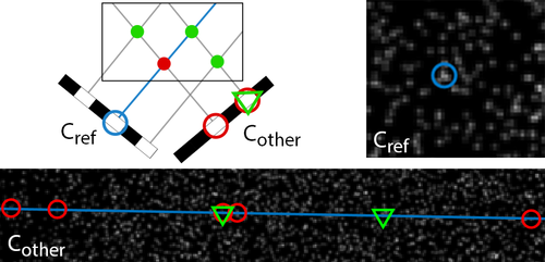
Figure 3: A particle in the reference camera (circle) can lead to multiple epipolar-consistent putative matches (circles). However, only a subset of them represents true 3D particles (triangles). Left: 1D-illustration. Right: peak in reference camera (0.1ppp). Bottom: other camera view with 5 putative matches that are consistent over all 4 cameras. Moreover, one true particle has initially not been found, due to visually overlapping ones that bias peak detection; but will be found in subsequent iterations, when the overlapping particles have been reconstructed and removed from the residual images or the triangulation threshold has been relaxed.

3.3 Energy Minimization

Our optimization is embedded in a two-fold coarse-to-fine scheme. On the one hand, we start with a larger value for $\sigma$, so as to increase the particles’ basins of attraction and improve convergence. During optimization, we progressively reduce $\sigma$ until we reach $\sigma=1$, meaning that a particle blob covers approximately the same area as in the input images. On the other hand, we also start at a coarser grid $\mathcal{Y}$ and refine the grid resolution along with $\sigma$.

To minimize the non-convex and non-smooth energy (4) for a given $\sigma$, we employ PALM (Bolte et al.,, 2014), in its inertial variant (Pock and Sabach,, 2016). Because our energy function is semi-algebraic (Bolte et al.,, 2014), it satisfies the Kurdyka-Lojasiewicz property (Bolte et al.,, 2007), therefore the sequence generated by PALM globally converges to a critical point of the energy. The key idea of PALM is to split the variables into blocks, such that the problem is decomposed into one smooth function on the entire variable set, and a sum of non-smooth functions in which each block is treated separately. We start by arranging the locations and intensities of the particles $\mathcal{Q}$ into two separate vectors $\mathbf{p}:=(p_{1}^{\!\mathsf{T}},\ldots,p_{Q}^{\!\mathsf{T}})^{\!\mathsf{T}}\in\mathbb{R}^{3Q}$ and $\mathbf{c}:=(c_{1},\ldots,c_{Q})^{\!\mathsf{T}}\in\mathbb{R}^{Q}$. Similarly, we stack the coefficients of the trilinear basis $\mathbf{u}:=(u_{\mathbf{i},1}^{\!\mathsf{T}},u_{\mathbf{i},2}^{\!\mathsf{T}},u_{\mathbf{i},3}^{\!\mathsf{T}})_{\mathbf{i}\in\mathcal{Y}}^{\!\mathsf{T}}\in\mathbb{R}^{3NML}$. With these groups, we split the energy functional into a smooth part $H$ and two non-smooth functions, $F_{\mathbf{c}}$ for the intensities $\mathbf{c}$ and $F_{\mathbf{u}}$ for the motion vectors $\mathbf{u}$:

$$\begin{split}&E(\mathbf{p},\mathbf{c},\mathbf{u}):=H(\mathbf{p},\mathbf{c},\mathbf{u})+F_{\mathbf{c}}(\mathbf{c})+F_{\mathbf{u}}(\mathbf{u})+F_{\mathbf{p}}(\mathbf{p}),\\ &\textrm{with}\\ &H(\mathbf{p},\mathbf{c},\mathbf{u}):=E_{D}(\mathbf{p},\mathbf{c},\mathbf{u})+\lambda\sum\nolimits_{l=1}^{3}\|\nabla\mathbf{u}_{l}\|^{2},\\ &F_{\mathbf{c}}(\mathbf{c}):=\mu E_{Sp}(\mathbf{c}),\\ &F_{\mathbf{u}}(\mathbf{u}):=\delta_{\{0\}}(\nabla\!\cdot\!\mathbf{u}),\\ &F_{\mathbf{p}}(\mathbf{p}):=0.\end{split}$$ (13)

For notation convenience, we define $F_{\mathbf{p}}(\mathbf{p}):=0$. The algorithm then alternates the steps of a proximal forward-backward scheme: take an explicit step w.r.t. one block of variables $z\in\{\mathbf{p},\mathbf{c},\mathbf{u}\}$ on the smooth part $H$ of the energy function, then take a backward (proximal) step on the non-smooth part $F_{z}$ w.r.t. the same variables. That is, we alternate steps of the form

$$\begin{split}z^{n+1}=\ &\textrm{prox}^{F_{z}}_{t}(z):=\operatorname*{arg\,min}_{y}F_{z}(y)+\frac{t}{2}\|y-z\|^{2},\\ &\textrm{ with }z=z^{n}-\frac{1}{t}\nabla_{z}H(\cdot,z^{n},\cdot),\end{split}$$ (14)

with a suitable step size $1/t$ for each block of variables. Here and in the following, the placeholder variable $z$ can stand for $\mathbf{c}$, $\mathbf{p}$ or $\mathbf{u}$, as required.

A key property is that, throughout the iterations, the partial gradient of function $H$ w.r.t. a variable block $z\in\{\mathbf{p},\mathbf{c},\mathbf{u}\}$ must be globally Lipschitz-continuous with some modulus $L_{z}$ at the current solution:

$$\|\nabla_{z}H(\cdot,z_{1},\cdot)-\nabla_{z}H(\cdot,z_{2},\cdot)\|\leq L_{z}(\cdot,\cdot)\|z_{1}-z_{2}\|\,\forall z_{1},z_{2}.$$ (15)

In other words, before we accept an update $z^{n+1}$ computed with (14), we need to verify that the step size $t$ in (14) fulfills the descent lemma (Bertsekas and Tsitsiklis,, 1989):

$$\begin{split}E(\cdot,z^{n+1},\cdot)\leq&E(\cdot,z^{n},\cdot)+\langle\nabla_{z}H(\cdot,z^{n},\cdot),z^{n+1}-z^{n}\rangle\\ &+\frac{t}{2}\|z^{n+1}-z^{n}\|^{2}.\end{split}$$ (16)

Note that Lipschitz continuity of the gradient of $H$ need not be tested globally, but can be verified locally at the current solution. This property allows for a back-tracking approach to determine the Lipschitz constant, e.g. Beck and Teboulle, (2009). Algorithm 1 provides pseudo-code for our scheme to minimize the energy (13). To accelerate convergence we apply extrapolation (lines 4/8/12). These inertial steps, c.f. Pock and Sabach, (2016); Beck and Teboulle, (2009), significantly reduce the number of iterations in the algorithm, while leaving the computational cost per step practically untouched. We also found it useful to not only reduce the step sizes (lines 7/11/15 in Alg. 1), but also to increase them, as long as (16) is fulfilled, so as to make the steps per iteration as large as possible.

Algorithm 1 iPalm implementation for energy (13)

1:procedure ipalm($\mathbf{p}^{0},\mathbf{c}^{0},\mathbf{u}^{0}$)

2:     $\mathbf{p}^{-1}\leftarrow\mathbf{p}^{0};\mathbf{c}^{-1}\leftarrow\mathbf{c}^{0};\mathbf{u}^{-1}\leftarrow\mathbf{u}^{0};$

3:     $\tau\leftarrow\frac{1}{\sqrt{2}};L_{\mathbf{p}}\leftarrow 1;L_{\mathbf{c}}\leftarrow 1;L_{\mathbf{u}}\leftarrow 1;$

4:     for n:=0 to $n_{\textrm{steps}}$ and while not converged do

5:         $\mathbf{\hat{p}}\leftarrow\mathbf{p}^{n}+\tau(\mathbf{p}^{n}-\mathbf{p}^{n-1});$ // inertial step

6:         while true do

7:              $\mathbf{p}^{n+1}:=\mathbf{\hat{p}}-1/L_{\mathbf{p}}\nabla_{\mathbf{p}}H(\mathbf{\hat{p}},\mathbf{c}^{n},\mathbf{u}^{n})$;

8:              if $\mathbf{p}^{n+1},L_{\mathbf{p}}$ fulfill (16) then break;

9:              else $L_{\mathbf{p}}=2L_{\mathbf{p}}$;                       

10:         $\mathbf{\hat{c}}\leftarrow\mathbf{c}^{n}+\tau(\mathbf{c}^{n}-\mathbf{c}^{n-1})$; // inertial step

11:         while true do

12:              $\mathbf{c}:=\mathbf{\hat{c}}-1/L_{\mathbf{c}}\nabla_{\mathbf{c}}H(\mathbf{p}^{n+1},\mathbf{\hat{c}},\mathbf{u}^{n});$

13:              $\mathbf{c}^{n+1}:=\textrm{prox}^{F_{\mathbf{c}}}_{L_{\mathbf{c}}}(\mathbf{c})$; // Eq. (14)

14:              if $\mathbf{c}^{n+1},L_{\mathbf{c}}$ fulfill (16) then break;

15:              else $L_{\mathbf{c}}=2L_{\mathbf{c}}$;                        

16:         $\mathbf{\hat{u}}\leftarrow\mathbf{u}^{n}+\tau(\mathbf{u}^{n}-\mathbf{u}^{n-1})$; // inertial step

17:         while true do

18:              $\mathbf{u}:=\mathbf{\hat{u}}-1/L_{\mathbf{u}}\nabla_{\mathbf{u}}H(\mathbf{p}^{n+1},\mathbf{c}^{n+1},\mathbf{\hat{u}})$;

19:              $\mathbf{u}^{n+1}:=\textrm{prox}^{F_{\mathbf{u}}}_{L_{\mathbf{u}}}(\mathbf{u})$; // Eq. (14)

20:              if $\mathbf{u}^{n+1},L_{\mathbf{u}}$ fulfill (16) then break;

21:              else $L_{\mathbf{u}}=2L_{\mathbf{u}}$;                             

One last thing needs to be explained, namely how we find the solution of the proximal steps on the intensities $\mathbf{c}$ and flow vectors $\mathbf{u}$. The former can be solved point-wise, leading to the following 1D-problem:

$$\textrm{prox}^{F_{c}}_{t}(\bar{c}):=\operatorname*{arg\,min}_{c}\mu|c|_{\diamond}+\delta_{\{\geq 0\}}(c)+\frac{t}{2}|c-\bar{c}|^{2},$$ (17)

which admits for a closed-form solution for both the $0$-norm $|c|_{0}$ and the $1$-norm $|c|_{1}$:

$$\textrm{prox}^{|\cdot|_{0}}_{t}(\bar{c}):=\left\{\begin{array}[]{c@{\hspace{0.2cm}}l}0\hfil\hskip 5.69046pt&\textrm{if }t\bar{c}^{2}<2\mu\textrm{ or }\bar{c}<0\\ \bar{c}\hfil\hskip 5.69046pt&\textrm{else},\end{array}\right.,$$ (18)

$$\textrm{prox}^{|\cdot|_{1}}_{t}(\bar{c}):=\max(0,\bar{c}-\mu/t).$$ (19)

The proximal step for the flow vector, $\textrm{prox}^{F_{\mathbf{u}}}_{t}(\mathbf{\bar{u}}):=\operatorname*{arg\,min}_{\mathbf{u}}\delta_{\{0\}}(\nabla\!\cdot\!\mathbf{u})+\frac{t}{2}\|\mathbf{u}-\mathbf{\bar{u}}\|^{2}$, requires the projection of $\mathbf{\bar{u}}$ onto the space of divergence-free 3D vector fields. Hence, given $\mathbf{\bar{u}}$, the solution is independent of the step size $1/t$, which we omit in the following. We construct the Lagrangian by introducing the multiplier $\mathbf{\phi}$, a scalar vector field whose physical meaning is the pressure in the fluid (Lasinger et al.,, 2017):

$$\min_{\mathbf{u}}\max_{\mathbf{\phi}}\frac{1}{2}\|\mathbf{u}-\mathbf{\bar{u}}\|^{2}+\mathbf{\phi}^{\!\mathsf{T}}\nabla\cdot\mathbf{u}.$$ (20)

To prevent confusion, we introduce $D\mathbf{u}$ as matrix notation for the linear divergence operator $(\nabla\!\cdot\!\mathbf{u})$ in (12). The KKT conditions of the Lagrangian yield a linear equation system. Simplification with the Schur complement leads to a Poisson system, which we solve for the pressure $\mathbf{\phi}$ to get the divergence-free solution:

$$\textrm{prox}^{F_{\mathbf{u}}}_{t}(\mathbf{\bar{u}}):=\mathbf{\bar{u}}-D^{\!\mathsf{T}}\mathbf{\phi}\quad\textrm{with }\;D^{\!\mathsf{T}}D\mathbf{\phi}=D^{\!\mathsf{T}}\mathbf{\bar{u}}.$$ (21)

Again interpreted physically, the divergence of the motion field is removed by subtracting the gradient of the resulting pressure field. For our problem of fluid flow estimation, it is not necessary to exactly solve the Poisson system in every iteration. Instead, we keep track of the pressure field $\mathbf{\phi}$ during optimization, and warm-start the proximal step. In this way, a few (10-20) iterations of preconditioned conjugate gradient descent suffice to update $\mathbf{\phi}$.

If we replace the hard divergence constraint with the soft penalty $E_{S,\alpha}$ from (11), we add $E_{S,\alpha}$ to the smooth function $H$ in (13). Then only the proximal step on the intensities $\mathbf{c}$ is needed in Alg. 1. We conclude by noting that accelerating the projection step is in itself an active research area in fluid simulation (Ladický et al.,, 2015; Tompson et al.,, 2016).

4 Evaluation

Since there is no other measurement technique that could deliver ground truth for fluid flow, we follow the standard practice and generate datasets for quantitative evaluation via direct numerical simulations (DNS) of turbulent flow, using the Johns Hopkins Turbulence Database (JHTDB) (Li et al.,, 2008; Perlman et al.,, 2007). This allows us to render realistic input images with varying particle densities and flow magnitudes, together with ground truth vectors on a regular grid. We evaluate how our approach performs with different smoothness terms, particle densities, initialization methods, particle sizes and temporal sampling rates. Additionally, we show results on “test case D” of the 4${}^{\text{th}}$ International PIV Challenge (Kähler et al.,, 2016) and quantitatively compare to the best performing method (Schanz et al.,, 2016).

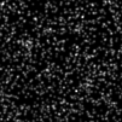
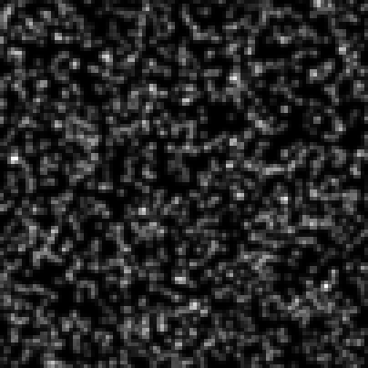
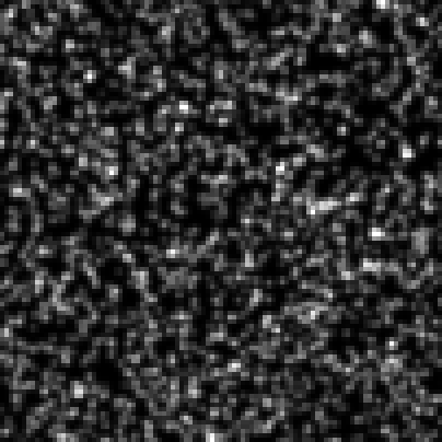
Figure 4: Detail of rendered 2D particle images for particle densities of 0.125, 0.175 and 0.225 ppp (from left to right).

Simulated dataset.

We follow the guidelines of the 4${}^{\text{th}}$ International PIV Challenge (Kähler et al.,, 2016) for the setup of our own dataset: Randomly sampled particles are rendered to four symmetric cameras of resolution $1500\times 800$ pixels, with viewing angles of $\pm 35^{\circ}$ w.r.t. the $yz$-plane of the volume, respectively $\pm 18^{\circ}$ w.r.t. the $xz$-plane. If not specified otherwise, particles are rendered as Gaussian blobs with $\sigma=1$ and varying intensity. We sample 12 datasets from 6 non-overlapping spatial and 2 temporal locations ($t=0.364$ and $t=8.364$) of the forced isotropic turbulence simulation of the JHTDB. Discretizing each DNS grid point with 4 voxels, identical to Kähler et al., (2016), each dataset corresponds to a volume size of $1024\times 512\times 352$. Standard temporal difference between two consecutive time steps is $\Delta t=0.004$. For each dataset we sample $480,000$ seeding particles at random locations within the volume and ground truth flow vectors at each DNS grid location. A subset of those particles is rendered on the actual camera views depending on the desired particle seeding density. In Fig. 4 we show $100\times 100$ patches of rendered camera views with seeding densities of $0.125$, $0.175$ and $0.225$ ppp. Note that with higher seeding densities particle occlusions and overlaps increase. For our flow fields with flow magnitudes up to $8.8$ voxels, we use $10$ pyramid levels with downsampling factor $0.94$. At every level we alternate between triangulation of candidate particles and minimization of the energy function (at most $40$ iteration per level).

The effective resolution of the reconstructed flow field is determined by the particle density. At a standard density of $\approx 0.1$ ppp and a depth range of $352$ voxels, we get a density of $\approx 0.0003$ particles per voxel. This suggests to estimate the flow on a coarser grid. We empirically found a particle density of $0.3$ per voxel to still deliver good results. Hence, we operate on a subsampled voxel grid of 10-times lower resolution per dimension in all our experiments, to achieve a notable speed-up and memory saving. The computed flow is then upsampled to the target resolution, with barely any loss of accuracy.

We always require a 2D intensity peak in all four cameras to instantiate a candidate particle. We start with a strict threshold of $\epsilon=0.8$ for the triangulation error, as suggested in (Wieneke,, 2013), which is relaxed to $\epsilon=2.0$ in later iterations. The idea is to first recover particles with strong support, and gradually add more ambiguous ones, as the residual images become less cluttered. We set $\lambda=0.04$ for our dataset. Since $\lambda$ corresponds to the viscosity it should be adapted for other fluids. We empirically set the sparsity weight $\mu=0.0001$.

Table 1: Endpoint error (AEE), angular error (AAE) and absolute divergence (AAD) for different regularizers (0.1 ppp).

	$E_{\textrm{S}}$	$E_{\textrm{S},64}$	$E_{\textrm{S},0}$	Lasinger et al., (2017)
AEE	0.136	0.135	0.157	0.406
AAE	2.486	2.463	2.870	6.742
AAD	0.001	0.008	0.100	0.001

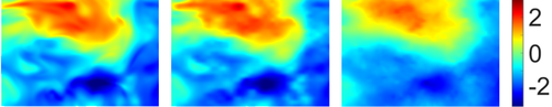
Figure 5: Detail from an $xy$-slice of the flow in $X$-direction. Left to right: Ground truth, our method and result of Lasinger et al., (2017).

Table 2: Influence of particle density on our joint approach, as well as several baselines.

ppp	IPR joint			IPR sequential			MART			true particles
	AEE	prec.	recall	AEE	prec.	recall	AEE	prec.	recall	AEE	prec.	recall
0.1	0.136	99.98	99.95	0.136	99.97	99.96	0.232	70.39	83.93	0.136	100	100
0.125	0.124	91.00	99.95	0.157	61.55	97.55	0.270	48.51	73.83	0.125	100	100
0.15	0.115	82.82	99.95	0.310	33.46	85.09	0.323	44.61	70.17	0.118	100	100
0.175	0.111	71.37	99.93	0.332	26.63	71.07	0.385	40.89	65.29	0.110	100	100
0.2	0.108	55.43	99.86	0.407	19.42	64.26	0.506	36.88	58.13	0.105	100	100
0.225	0.113	34.39	99.87							0.101	100	100
0.25	0.134	24.54	99.51							0.098	100	100

Regularization.

Our framework allows us to plug in different smoothness terms. We show results for hard ($E_{\textrm{S}}$) and soft divergence regularization ($E_{\textrm{S},\alpha}$). Average endpoint error (AEE), average angular error (AAE), and average absolute divergence (AAD) are displayed in Tab. 1. Compared to our default regularizer $E_{\textrm{S}}$, removing the divergence constraint ($\alpha=0$), increases the error by $\approx 15\%$. With the soft constraint at high $\alpha=64$, the results are equal to those of $E_{\textrm{S}}$. We also compare to our previous sequential Eulerian-based approach (Lasinger et al.,, 2017). Our joint model improves the performance by $\approx 70\%$ over that recent baseline, on both error metrics. In Fig. 5 we visually compare our results (with hard divergence constraint) to those of Lasinger et al., (2017). The figure shows the flow in $X$-direction in one particular $xy$-slice of the volume. Our method recovers a lot finer details, and is clearly closer to the ground truth.

Particle Density & Initialization Method.

There is a trade-off for choosing the seeding density: A higher density raises the observable spatial resolution, but at the same time makes matching more ambiguous. This causes false positives, commonly called “ghost particles”. Very high densities are challenging for all known reconstruction techniques. The additive image formation model of Eq. (5) also suggests an upper bound on the maximal allowed particle density. Tab. 2 reports results for varying particle densities. We measure recall (fraction of reconstructed ground truth particles) and precision (fraction of reconstructed particles that coincide with true particles to $<1$ pixel). In Fig. 6 visualizations of our estimated flow fields for two different particle densities are shown.

To provide an upper bound, we initialize our method with ground truth particle locations at time step 0 and optimize only for the flow estimation. We also evaluate a sequential version of our method, in which we separate energy (4) into particle reconstruction and subsequent motion field estimation. In addition to our proposed IPR-like triangulation, we initialize particles with the popular volumetric tomography method MART (Elsinga et al.,, 2006). MART creates a full, high-resolution voxel grid of intensities (with, hopefully, lower intensities for ghost particles and very low ones in empty space). To extract a set of sub-voxel accurate 3D particle locations we perform peak detection, similar to the 2D case for triangulation. Since MART always returns the same particle set we run it only once, but increase the number of iterations for the minimizer from $40$ to $160$.

Starting from a perfect particle reconstruction (true particles) the flow estimate improves with increasing particle density. Remarkably, our proposed iterative triangulation approach achieves results comparable to the ground truth initialization, up to high particle densities and is able to resolve most particle ambiguities. In contrast, MART and the sequential baseline struggle with increasing particle density, which supports our claim that joint energy minimization can better reconstruct the particles.

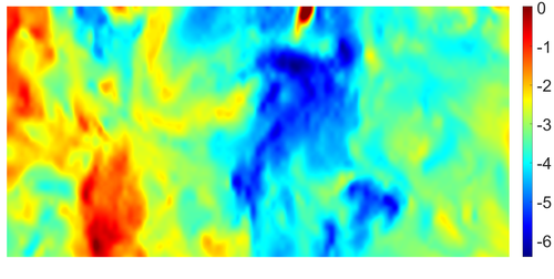
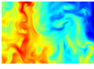
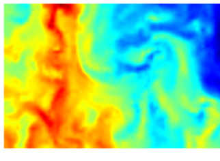
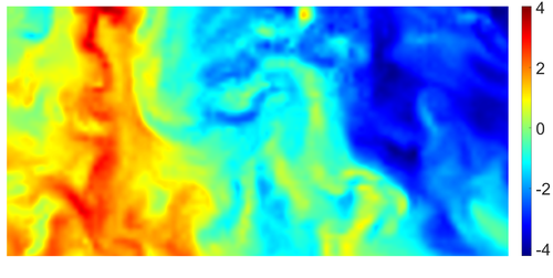
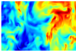
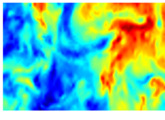
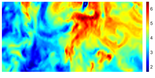
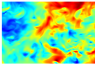
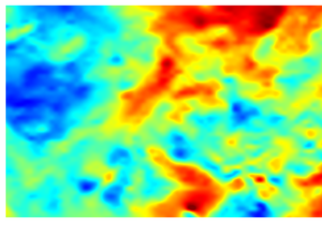
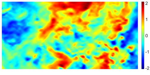
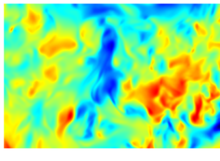
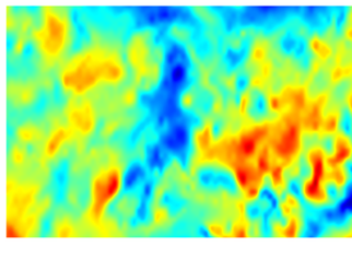
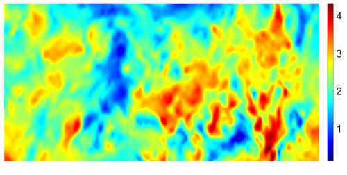
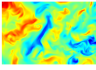
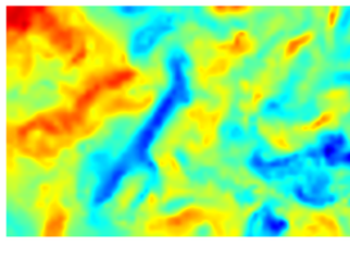
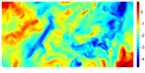
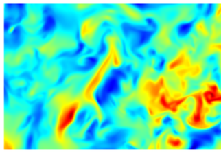
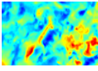
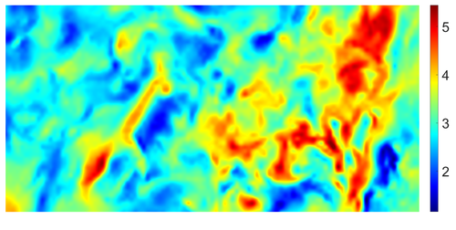
Figure 6: Visualization of center $xy$-slice ($z=176$) of the flow for two of our tested datasets. Left to right: Ground truth, $0.0125$ppp, $0.0225$ppp. Top to bottom: X-,Y-,Z-component and magnitude. Note that with higher particle density details are recovered better, but the method starts to fail in certain areas (see highlighted areas in first row).

Sparsity Term.

In Tab. 3 we show a comparison between the two proposed sparsity norms and their influence on precision of the particle reconstruction and the flow endpoint error. The 0-norm performs slightly better than the 1-norm by eliminating more ghost particles that occur at high seeding densities.

Particle Size.

For the above experiments, we have rendered the particles into the images as Gaussian blobs with fixed $\sigma=1$, and the same is done when re-rendering for the data term, respectively, proposal generator. We now test the influence of particle size on the reconstruction, by varying $\sigma$. Tab. 4 shows results with hard divergence constraint and fixed particle density $0.1$, for varying $\sigma\in[0.6\ldots 1.6]$. For small enough particles, size does not matter, very large particles lead to more occlusions and degrade the flow. Furthermore, we verify the sensitivity of the method to unequal particle size. To that end, we draw an individual $\sigma$ for each particle from the normal distribution $\mathcal{N}(1,0.1^{2})$, while still using a fixed $\sigma=1$ during inference. As expected, the mismatch between actual and rendered particles causes slightly larger errors.

Temporal Sampling.

To quantify the stability of our method to different flow magnitudes we modify the time interval between the two discrete time steps and summarize the results in Tab. 5, together with the respective maximum flow magnitude $|u|_{2}$. For lower frame rate (1.25x and 1.5x), and thus larger magnitudes, we set our pyramid downsampling factor to $0.93$.

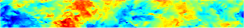
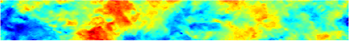
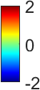
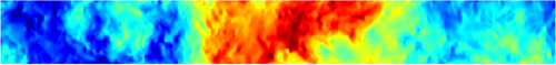
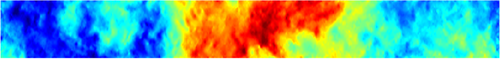
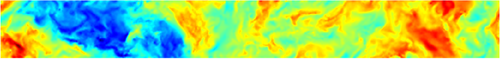
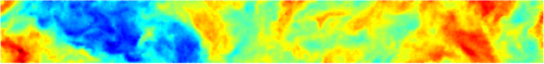
Figure 7: $xy$-slice of the flow field for snapshot 10 of the 4${}^{\text{th}}$ PIV Challenge. Top to bottom: $X,Y,Z$ flow components. Left: multi-frame StB Schanz et al., (2016). Right: our 2-frame method.

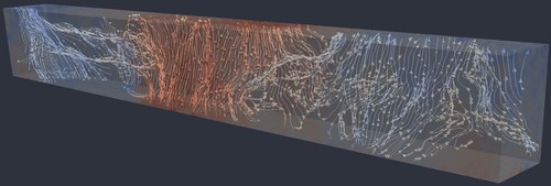
Figure 8: PIV Challenge: Streamline visualizations of our results for snapshot 10 of the 4${}^{\text{th}}$ PIV Challenge Kähler et al., (2016) with y component of the flow color coded.

Table 3: Influence of different sparsity norms: 0-norm vs. 1-norm ($0.2$ ppp).

Norm	$|\cdot|_{0}$	$|\cdot|_{1}$
AEE	0.108	0.110
prec.	55.43	25.23
recall	99.86	99.94

Table 4: Influence of particle size on reconstruction quality (0.1 ppp).

$\sigma$	0.6	0.8	1	1.2	1.4	1.6	$\mathcal{N}_{1,0.1^{2}}$
AEE	0.194	0.135	0.136	0.140	0.217	0.235	0.155
AAE	3.388	2.465	2.486	2.561	4.002	4.575	2.879

Table 5: Varying the sampling distance between frames ($0.1$ ppp).

Temp. dist.	0.75x	1.0x	1.25x	1.5x
AEE	0.102	0.136	0.170	0.283
Max. $|u|_{2}$	6.596	8.795	10.993	13.192

PIV Challenge.

Unfortunately, no ground truth is provided for the data of the 4${}^{\text{th}}$ PIV Challenge Kähler et al., (2016), such that we cannot run a quantitative evaluation on that dataset. However, Schanz et al., (2016) kindly provided us results for their method, StB, for snapshot 10. StB was the best-performing method in the challenge with an endpoint error of $\approx$0.24 voxels (compared to errors $>$0.3 for all competitors). The average endpoint difference between our approach and StB is $<$0.14 voxels. In Fig. 7 both results appear to be visually comparable, yet, note that StB includes a tracking procedure that requires data of multiple time steps ($15$ for the given particle density $0.1$). Fig. 8 shows a streamline visualization of our results at snapshot 10.

5 Experimental Data

We show qualitative results of two experiments in both air and water, utilizing the pinhole camera model and the polynomial camera model respectively.

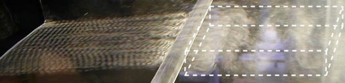
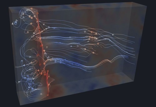
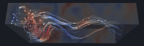
Figure 9: Experimental setup in air: Top: Karman street behind cylinder. Middle and bottom: Streamline visualizations of our results with color coding based on z component of the flow (where the Karman street can be observed best).

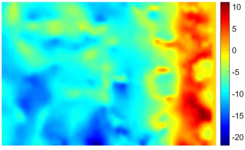
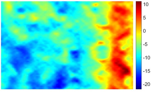
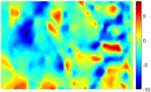
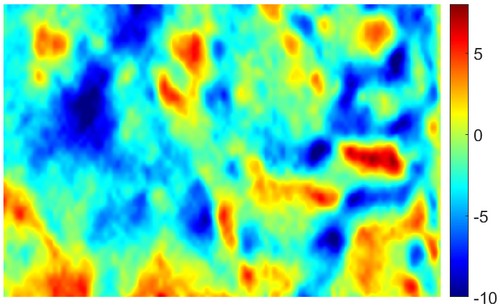
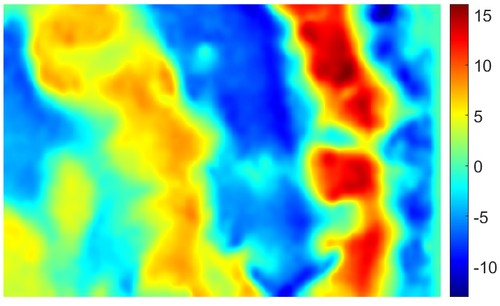
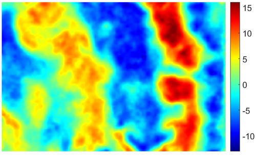
Figure 10: Experimental setup in air: $xy$-slice of the flow at $z=203$. Left: Reference flow field provided by LaVision (TomoPIV). Right: Results with our approach. (top to bottom: flow in $X$, $Y$ and $Z$-direction).

Experiment in air.

We test our approach on experimental data provided by LaVision (see Michaelis et al., (2006)). The experiment captures the wake flow behind a cylinder, which forms a so-called Karman vortex street (see Fig. 1 and 9). Data is provided in form of a tomographic reconstruction of the particle volume. In order to run our method, we backproject the particle volume to four arbitrary camera views (we take the same as for our simulated dataset) and use those backprojected images as input to our method. Since particle densities allow it and the provided reference flow is of low resolution, we downsample the input volume by a factor of 2 from $2107\times 1434\times 406$ to $1054\times 717\times 203$ and render to 2D images of dimensions $1500\times 1100$ with particle size $\sigma=0.6$. Note, that since those camera locations do not necessarily coincide with the original camera locations, ghost particles in the reconstructed volume may lead to wrong particles in the backprojected image. However, as results in Fig. 10 indicate, our algorithm is able to recover a detailed flow field that corresponds with the reference flow despite these deflections in the data. In addition to our own result, we show results provided by LaVision. The provided reference flow field was estimated with TomoPIV (Elsinga et al.,, 2006), using a final interrogation volume size of $48^{3}$ and an overlap of $75\%$, i.e. one flow vector at every 12 voxel locations. It can be seen in Fig. 10 that our method recovers much finer details of the flow, due to the avoidance of large interrogation volumes. In order to cope with flow magnitudes up to 15.5 voxel we chose 16 pyramid levels and a pyramid downsampling factor of $0.92$. Note, that in the resulting flow field the cylinder is positioned to the right of the volume and the general flow direction is towards the left. Effects of the Karman vortex street can be primarily seen in the z component of the flow (periodically alternating flow directions with decreasing magnitude from right to left).

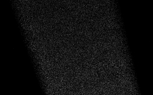
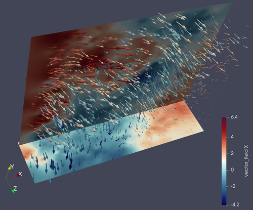
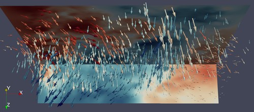
Figure 11: Experimental setup in water: Top: Input camera image for one view. Bottom: Visualization of flow vectors with X-flow for color coding and flow magnitude for vector size.

Experiment in water.

To test our polynomial camera model we show results of an isotropic turbulence experiment in water. The experimental setup includes a cylinder filled with water and two discs, located on the top and bottom of the cylinder, which are rotating in opposite direction. This setup is also known as French washing machine. The rotating discs lead to a turbulent flow, with multiple rotational patterns. In Fig. 11 we show one of the input camera images together with visualizations of the resulting flow field, obtained from two time steps. The arrow size encodes the magnitude of the flow and the color denotes its motion in X-direction (red positive, blue negative). One can see a clock-wise rotating vortex on the left side of the volume and a counter-clockwise rotating vortex with lower magnitude on the right. The camera was calibrated from 20000 point correspondences, which were kindly provided together with the data by Daniel Schanz (DLR). Following Hartley and Saxena, (1997), we use DLT to get an initial estimate of the 38 parameters of the polynomial camera model and optimize the result using the iterative Levenberg-Marquardt method. Input images have a resolution of $2560\times 2600$. Based on the given point correspondences and the image resolution we chose a down-sampled volume of $162\times 114\times 36$ voxels for our motion field estimation.

6 Conclusion

We have presented the first variational model that jointly solves sparse particle reconstruction and dense 3D fluid motion estimation in PIV/PTV data for the common multi-camera setup. The sparse particle representation allows us to utilize the high-resolution image data for matching, while keeping memory consumption low enough to process large volumes. Densely modeling the fluid motion in 3D enables the direct use of physically motivated regularizers, in our case viscosity and incompressibility. The proposed joint optimization captures the mutual dependencies between particle reconstruction and flow estimation. This yields results that are clearly superior to traditional, sequential methods (Elsinga et al.,, 2006; Lasinger et al.,, 2017); and, using only 2 frames, competes with the best available multi-frame methods, which require sequences of 15-30 time steps. We have validated the performance of our approach both quantitatively on synthetic data and qualitatively on real experiments in water and air.

In our experiments we have demonstrated that the proposed joint formulation allows for much higher seeding densities than traditional sequential approaches, by implicitly utilizing information of both time steps also for the particle reconstruction, thus reducing the amount of wrongly reconstructed ghost particles.

One limitation of our current regularization scheme is that it does not account for turbulent (non-Stokes) flow of high Reynolds numbers. Here, an extension in the spirit of Ruhnau and Schnörr, (2007) could be a promising future direction. Another interesting extension is to put more focus also on the recovery of the pressure field. To that end one might again follow Ruhnau and Schnörr, (2007) and move to a discretization scheme with mixed finite elements, which fulfills the Babuska-Brezzi condition (Brezzi and Fortin,, 1991). Our approach could further be extended to more than two time steps to even better exploit temporal consistency. Besides resolving some of the remaining ambiguities of the particle reconstruction, this would also facilitate the use of additional physical constraints, e.g., incorporating the transport equations (inertial part) of the Navier-Stokes model (c.f. Ruhnau et al.,, 2006). Such an integrated model over multiple time steps will considerably increase the computational cost, and may require additional efforts to make energy minimization more efficient. Also, when dealing with longer sequences one will have to account for the possibility that particles enter or leave the measurement volume, and for particles’ intensity changes over time.

Acknowledgements.

This work was supported by ETH grant 29 14-1. Thomas Pock and Christoph Vogel acknowledges support from the ERC starting grant 640156, ’HOMOVIS’. We thank Daniel Schanz for kindly sharing their results on the 4th PIV Challenge and for providing experimental data in water.

References

- Adams et al., (2007) Adams, B., Pauly, M., Keiser, R., and Guibas, L. J. (2007). Adaptively sampled particle fluids. ACM SIGGRAPH.
- Adrian and Westerweel, (2011) Adrian, R. and Westerweel, J. (2011). Particle Image Velocimetry. Cambridge University Press.
- Atkinson and Soria, (2009) Atkinson, C. and Soria, J. (2009). An efficient simultaneous reconstruction technique for tomographic particle image velocimetry. Experiments in Fluids, 47(4).
- Barbu et al., (2013) Barbu, I., Herzet, C., and Mémin, E. (2013). Joint Estimation of Volume and Velocity in TomoPIV. In 10th Int’l Symp. on Particle Image Velocimetry - PIV13.
- Basha et al., (2010) Basha, T., Moses, Y., and Kiryati, N. (2010). Multi-view scene flow estimation: a view centered variational approach. CVPR.
- Beck and Teboulle, (2009) Beck, A. and Teboulle, M. (2009). A fast iterative shrinkage-thresholding algorithm for linear inverse problems. SIAM journal on imaging sciences, 2(1).
- Bertsekas, (1999) Bertsekas, D. (1999). Nonlinear Programming. Athena Scientific.
- Bertsekas and Tsitsiklis, (1989) Bertsekas, D. P. and Tsitsiklis, J. N. (1989). Parallel and Distributed Computation: Numerical Methods. Prentice-Hall.
- Bolte et al., (2007) Bolte, J., Daniilidis, A., and Lewis, A. (2007). The Lojasiewicz inequality for nonsmooth subanalytic functions with applications to subgradient dynamical systems. SIAM J Optimiz, 17(4).
- Bolte et al., (2014) Bolte, J., Sabach, S., and Teboulle, M. (2014). Proximal alternating linearized minimization for nonconvex and nonsmooth problems. Math Programming, 146(1).
- Boyd and Vandenberghe, (2004) Boyd, S. and Vandenberghe, L. (2004). Convex Optimization. Cambridge University Press, New York, NY, USA.
- Brezzi and Fortin, (1991) Brezzi, F. and Fortin, M. (1991). Mixed and Hybrid Finite Element Methods. Springer-Verlag, Berlin, Heidelberg.
- Champagnat et al., (2011) Champagnat, F., Plyer, A., Le Besnerais, G., Leclaire, B., Davoust, S., and Le Sant, Y. (2011). Fast and accurate PIV computation using highly parallel iterative correlation maximization. Experiments in Fluids, 50(4).
- Cheminet et al., (2014) Cheminet, A., Leclaire, B., Champagnat, F., Plyer, A., Yegavian, R., and Le Besnerais, G. (2014). Accuracy assessment of a lucas-kanade based correlation method for 3D PIV. In Int’l Symp. Applications of Laser Techniques to Fluid Mechanics.
- Courant, (1943) Courant, R. (1943). Variational methods for the solution of problems of equilibrium and vibrations. Bulletin of the American Mathematical Society, 49(1).
- Dalitz et al., (2017) Dalitz, R., Petra, S., and Schnörr, C. (2017). Compressed motion sensing. SSVM.
- Discetti and Astarita, (2012) Discetti, S. and Astarita, T. (2012). Fast 3D PIV with direct sparse cross-correlations. Experiments in Fluids, 53(5).
- Elsinga et al., (2006) Elsinga, G. E., Scarano, F., Wieneke, B., and Oudheusden, B. W. (2006). Tomographic particle image velocimetry. Experiments in Fluids, 41(6).
- Gesemann et al., (2016) Gesemann, S., Huhn, F., Schanz, D., and Schröder, A. (2016). From noisy particle tracks to velocity, acceleration and pressure fields using B-splines and penalties. Int’l Symp. on Applications of Laser Techniques to Fluid Mechanics.
- Gregson et al., (2014) Gregson, J., Ihrke, I., Thuerey, N., and Heidrich, W. (2014). From capture to simulation: connecting forward and inverse problems in fluids. ACM ToG, 33(4).
- Hartley and Saxena, (1997) Hartley, R. I. and Saxena, T. (1997). The cubic rational polynomial camera model. In In Image Understanding Workshop.
- Huguet and Devernay, (2007) Huguet, F. and Devernay, F. (2007). A variational method for scene flow estimation from stereo sequences. ICCV.
- Kähler et al., (2016) Kähler, C. J. et al. (2016). Main results of the 4th International PIV Challenge. Experiments in Fluids, 57(6).
- Ladický et al., (2015) Ladický, L., Jeong, S., Solenthaler, B., Pollefeys, M., and Gross, M. (2015). Data-driven fluid simulations using regression forests. ACM ToG, 34(6).
- Langtangen et al., (2002) Langtangen, H. P., Mardal, K.-A., and Winther, R. (2002). Numerical methods for incompressible viscous flow. Advances in Water Resources, 25(8).
- Lasinger et al., (2018) Lasinger, K., Vogel, C., Pock, T., and Schindler, K. (2018). Variational 3d-PIV with sparse descriptors. Measurement Science and Technology, 29(6).
- Lasinger et al., (2019) Lasinger, K., Vogel, C., Pock, T., and Schindler, K. (2019). 3d fluid flow estimation with integrated particle reconstruction. GCPR.
- Lasinger et al., (2017) Lasinger, K., Vogel, C., and Schindler, K. (2017). Volumetric flow estimation for incompressible fluids using the stationary stokes equations. ICCV.
- Li et al., (2008) Li, Y. et al. (2008). A public turbulence database cluster and applications to study Lagrangian evolution of velocity increments in turbulence. J. of Turbulence, 9.
- Maas et al., (1993) Maas, H. G., Gruen, A., and Papantoniou, D. (1993). Particle tracking velocimetry in three-dimensional flows. Experiments in Fluids, 15(2).
- Menze and Geiger, (2015) Menze, M. and Geiger, A. (2015). Object scene flow for autonomous vehicles. CVPR.
- Michaelis et al., (2006) Michaelis, D., Poelma, C., Scarano, F., Westerweel, J., and Wieneke, B. (2006). A 3d time-resolved cylinder wake survey by tomographic piv. In ISFV12.
- Michalec et al., (2015) Michalec, F.-G., Schmitt, F., Souissi, S., and Holzner, M. (2015). Characterization of intermittency in zooplankton behaviour in turbulence. European Physical J, 38(10).
- Monaghan, (2005) Monaghan, J. J. (2005). Smoothed particle hydrodynamics. Reports on Progress in Physics, 68(8).
- Perlman et al., (2007) Perlman, E., Burns, R., Li, Y., and Meneveau, C. (2007). Data exploration of turbulence simulations using a database cluster. In Conf. on Supercomputing.
- Petra et al., (2009) Petra, S., Schröder, A., and Schnörr, C. (2009). 3d tomography from few projections in experimental fluid dynamics. In Imaging Meas. Methods for Flow Analysis.
- Pock and Sabach, (2016) Pock, T. and Sabach, S. (2016). Inertial proximal alternating linearized minimization (iPALM) for nonconvex and nonsmooth problems. SIAM J Imaging Sci, 9(4).
- Rabe et al., (2010) Rabe, C., Müller, T., Wedel, A., and Franke, U. (2010). Dense, robust, and accurate motion field estimation from stereo image sequences in real-time. ECCV.
- Raffel et al., (2018) Raffel, M., Willert, C. E., Wereley, S., and Kompenhans, J. (2018). Particle image velocimetry: a practical guide. Springer.
- Reddy, (1993) Reddy, J. N. (1993). An introduction to the finite element method. New York.
- Richard et al., (2017) Richard, A., Vogel, C., Blaha, M., Pock, T., and Schindler, K. (2017). Semantic 3d reconstruction with finite element bases. In BMVC.
- Ruhnau et al., (2005) Ruhnau, P., Guetter, C., Putze, T., and Schnörr, C. (2005). A variational approach for particle tracking velocimetry. Measurement Science and Technology, 16(7).
- Ruhnau and Schnörr, (2007) Ruhnau, P. and Schnörr, C. (2007). Optical stokes flow estimation: an imaging-based control approach. Experiments in Fluids, 42(1).
- Ruhnau et al., (2006) Ruhnau, P., Stahl, A., and Schnörr, C. (2006). On-line variational estimation of dynamical fluid flows with physics-based spatio-temporal regularization. GCPR.
- Schanz et al., (2016) Schanz, D., Gesemann, S., and Schröder, A. (2016). Shake-The-Box: Lagrangian particle tracking at high particle image densities. Experiments in Fluids, 57(5).
- Schanz et al., (2012) Schanz, D., Gesemann, S., Schröder, A., Wieneke, B., and Novara, M. (2012). Non-uniform optical transfer functions in particle imaging: calibration and application to tomographic reconstruction. Measurement Science & Technology, 24(2).
- Schneiders and Scarano, (2016) Schneiders, J. F. and Scarano, F. (2016). Dense velocity reconstruction from tomographic PTV with material derivatives. Exp. in Fluids, 57(9).
- Soloff et al., (1997) Soloff, S. M., Adrian, R. J., and Liu, Z.-C. (1997). Distortion compensation for generalized stereoscopic particle image velocimetry. Measurement Science and Technology.
- Taylor and Hood, (1973) Taylor, C. and Hood, P. (1973). A numerical solution of the Navier-Stokes equations using the finite element technique. Computers & Fluids, 1(1).
- Tompson et al., (2016) Tompson, J., Schlachter, K., Sprechmann, P., and Perlin, K. (2016). Accelerating eulerian fluid simulation with convolutional networks. CoRR, abs/1607.03597.
- Valgaerts et al., (2010) Valgaerts, L., Bruhn, A., Zimmer, H., Weickert, J., Stoll, C., and Theobalt, C. (2010). Joint estimation of motion, structure and geometry from stereo sequences. ECCV.
- Vogel et al., (2011) Vogel, C., Schindler, K., and Roth, S. (2011). 3D scene flow estimation with a rigid motion prior. ICCV.
- Vogel et al., (2013) Vogel, C., Schindler, K., and Roth, S. (2013). Piecewise rigid scene flow. ICCV.
- Vogel et al., (2015) Vogel, C., Schindler, K., and Roth, S. (2015). 3D scene flow estimation with a piecewise rigid scene model. IJCV, 115(1).
- Wedel et al., (2011) Wedel, A., Brox, T., Vaudrey, T., Rabe, C., Franke, U., and Cremers, D. (2011). Stereoscopic scene flow computation for 3d motion understanding. IJCV, 95(1).
- Wieneke, (2008) Wieneke, B. (2008). Volume self-calibration for 3d particle image velocimetry. Experiments in fluids, 45(4).
- Wieneke, (2013) Wieneke, B. (2013). Iterative reconstruction of volumetric particle distribution. Measurement Science & Technology, 24(2).
- Wu et al., (2009) Wu, Z., Hristov, N., Hedrick, T., Kunz, T., and Betke, M. (2009). Tracking a large number of objects from multiple views. ICCV.
- Xiong et al., (2017) Xiong, J., Idoughi, R., Aguirre-Pablo, A. A., Aljedaani, A. B., Dun, X., Fu, Q., Thoroddsen, S. T., and Heidrich, W. (2017). Rainbow particle imaging velocimetry for dense 3d fluid velocity imaging. ACM Trans. Graph., 36(4).
- Zhu and Bridson, (2005) Zhu, Y. and Bridson, R. (2005). Animating sand as a fluid. ACM ToG, 24(3).