Image Moment Models for Extended Object Tracking

Abstract

In this paper, a novel image moments based model for shape estimation and tracking of an object moving with a complex trajectory is presented. The camera is assumed to be stationary looking at a moving object. Point features inside the object are sampled as measurements. An ellipsoidal approximation of the shape is assumed as a primitive shape. The shape of an ellipse is estimated using a combination of image moments. Dynamic model of image moments when the object moves under the constant velocity or coordinated turn motion model is derived as a function for the shape estimation of the object. An Unscented Kalman Filter-Interacting Multiple Model (UKF-IMM) filter algorithm is applied to estimate the shape of the object (approximated as an ellipse) and track its position and velocity. A likelihood function based on average log-likelihood is derived for the IMM filter. Simulation results of the proposed UKF-IMM algorithm with the image moments based models are presented that show the estimations of the shape of the object moving in complex trajectories. Comparison results, using intersection over union (IOU), and position and velocity root mean square errors (RMSE) as metrics, with a benchmark algorithm from literature are presented. Results on real image data captured from the quadcopter are also presented.

I Introduction

Traditional target tracking literature[1], such as simultaneous localization and mapping (SLAM) [2, 3], structure from motion (SfM) [4, 5] and target tracking [6], models the targets as point targets. Once the estimation is performed, another layer of optimization is used to estimate the shape of the target. With the increased resolution of the modern sensors, such as phased array radar, laser range finder, 2D/3D cameras, the sensors are capable of giving more than one point measurement from an observed target at a single time instance. For instance, in a camera image, multiple SIFT/SURF points can be obtained inside a chosen region of interest (ROI) or 3D cameras, such as Kinect camera gives a collection of points in a given ROI. The multiple measurements from a target can be used to estimate and track not only the position and velocity of the centroid but also its spatial extent. The combined target tracking and shape estimation is commonly referred to as an extended object tracking (EOT) problem [7, 8].

Multiple feature points such as SIFT and SURF points can not be identified consistently and tracked individually over long period of time inside an object or multiple objects. With multiple noisy measure points generated from the target at each time step without association, the target can be roughly estimated as an ellipse shape, which will provide the kinematic (position and velocity of the centroid) and spatial extent information (orientation and size) useful for real world applications. The extended object is modeled by stick [9], Gaussian mixture model [10], rectangle [11], Gaussian process model [12], and splines [13]. Two widely used models to represent targets with spatial extent are random matrix model (RMM) [14] and elliptic random hyper-surface model (RHM) [15], where the true shape of the object is approximated by an ellipse. In RMM, the shape of the target object is represented by using a symmetric positive definite (SPD) matrix. The elements of the matrix along with the centroid of the object are used as a state vector, which is estimated by using a filter. Multiple improvements to the RMM model are presented in literature [16, 17, 18, 19]. The situation when the measurement noise is comparable to the extent of the target and can not be neglected is considered in [16, 20]. Considering the target will change the size and shape abruptly especially during the maneuvering movement, the rotation matrix or scaling matrix is multiplied on both sides of the positive symmetric matrix and the corresponding filters are derived in [17, 18, 19]. The RHM model assumes each measurement source lies on a scaled version of the true ellipse describing the object, and the extent of the object is represented by the entries from the Cholesky decomposition of the SPD matrix [21, 22, 23]. In [24], a multiplicative noise term in the measurement equation is used to model the spatial distribution of the measurements and a second order extended Kalman filter is derived for a closed form recursive measurement update. In [25], comparisons between the RHM with RMM are illustrated. RHM with Fourier series expansion and level-set are applied for modeling star-convex and non-convex shapes, respectively [23, 26]. By approximating the complex shapes as the combination of multiple ellipse sub-objects, the elliptic RMMs are investigated to model irregular shapes [17, 27]. A comprehensive overview of the extended object tracking can be found in [8, 7].

The dynamic model for a moving extended object describes how the target’s kinematic parameters and extent evolve over time. For tracking a point object, the kinematic parameters such as position, velocity or acceleration can fully describe the state of the object. However, for an extended object, the object shape estimation is also important, especially when the target conducts maneuvering motion or the shape of the extended target changes abruptly. For tracking extended object using RMM, there is no explicit dynamic model and the update for the extent is based on simple heuristics which increase the extent’s covariance, while keeping the expected value constant [14]. An alternative to the heuristic update is to use Wishart distribution to approximate the transition density of the spatial extent [14, 28, 18]. The prediction update of extended targets within the RMM framework is explored by multiplying the rotation matrix or scaling matrix on the both sides of the positive symmetric matrix in [19, 18]. In [18], a comprehensive comparison results between four process models are presented. For tracking elliptic extended object using RHM, the covariance matrix of the uncertainty of the object’s shape parameters is increased at each time step to capture the variations in the shape [15].

Image moments have found a wide use in tracking, visual servoing and pattern recognition [29, 30, 2, 31]. Hu’s moments [32] invariant under translation, rotation and scaling of the object, are widely investigated in pattern recognition. In this paper, an alternative representation, using image moments, to describe an ellipse shape that can be used to approximate an extended object is presented. Dynamic models of image moments that are used to represent an extended object for the target moving in an uniform motion and a coordinated turn motion are presented. The image moments based RHM is used with the interacting multiple model (IMM) approach [33, 34, 35] for tracking extended target undergoing complex trajectories. A novel likelihood function based on average log-likelihood is derived for the IMM. An unscented Kalman filter (UFK) is used to estimate the states of each individual model of the UKF-IMM filter. The UKF-IMM approach assumes the target obeys one of the finite number of motion models and identifies the beginning and the end of the motion models by updating the mode probabilities. The adaptation via model probability update of the UKF-IMM approach keeps the estimation errors low, both during maneuvers as well as non-maneuver intervals. The contributions of the paper are briefly summarized as follows:

• The minimal, complete, and non-ambiguous representation of an elliptic object based on image moments is presented for extended object tracking. UKF-IMM filter is adopted based on the multiple dynamic models and corresponding image moments based RHM.

• A novel method of calculating the likelihood function, based on average log-likelihood of the image moments based RHM, is proposed for the UKF-IMM filter. In order to estimate the model probability consistently, the calculation of the average log-likelihood function by unscented transformation is proposed.

• Results of the UKF-IMM filter with the image moments based model are presented and compared with a benchmark algorithm to validate the performance of the proposed approach.

Rest of the paper is organized as follows. In Section II, the image moments based random hypersurface model is proposed to approximate an elliptic object and its dynamic models are analytically derived. Following the framework of the random hypersurface model, the measurement model is also provided. in Section III, the Bayesian inference of the position, velocity and extent of the object from the noisy measurement points uniformly generated from the object is illustrated. Since the dynamic or measurement model is nonlinear, UKF is applied to estimate the extended object. For tracking the moving target switching between maneuvering and non-maneuvering motions, the proposed image moments based RHM is embedded within the framework of the interacting multiple model (IMM) in section IV. The UKF-IMM algorithm is illustrated with the proposed image moments based RHM, and the algorithm for the calculation of the likelihood function by using the average log-likelihood function and unscented transformation is also proposed. In section V, the proposed image moments based RHM with its dynamic models is evaluated in three tests: (1) static scenario for validating the measurement model; (2) constant velocity and coordinated turn motion to validate the dynamic models; (3) two complex trajectories are used to validate the UKF-IMM algorithm with the proposed image moments based RHM, and its performance is compared with the RMM models in [20] as the benchmark. The estimation results show that the proposed model provides comparable and accurate results. In Section VI, the proposed algorithm is applied for tracking a moving car with the real trajectory. Conclusion and future work are given in Section VII. To improve legibility, the subindices, such as the time step $k$ and the measurement number $l$ will be dropped unless needed in the following.

II Image Moments based Random Hypersurface Model

II-A Representation of the Ellipse using Image Moments

In this section, a generalized representation of the ellipse using image moments is presented. The $(i+j\mathrm{)th}$ moment of an object $m_{ij}$ in a 2D plane is defined by [29]

$$m_{ij}=\iintop_{R(t)}x^{i}y^{j}dxdy,\;\>\forall\,i,j\in\mathbb{N}$$ (1)

where $R(t)$ is the surface of the object and $\mathbb{N}$ is a set of natural numbers. The centered moment is defined as [29]

$$\eta_{ij}=\iintop_{R(t)}h(\bar{x},\bar{y})dxdy$$ (2)

where $h(\bar{x},\bar{y})=(\bar{x})^{i}(\bar{y})^{j}$, $\bar{x}=x-x_{c}$, $\bar{y}=y-y_{c}$ and $(x_{c,}y_{c})$ is the centroid of the object.

Any point on the surface of the object can be represented as a point located on the boundary of the scaled ellipse. The general equation of a family of ellipses in terms of semi-major, and semi-minor axes, centroid, and orientation is given by

$$\frac{(x-x_{c}+t(y-y_{c}))^{2}}{a_{1}^{2}(1+t^{2})}+\frac{(y-y_{c}-t(x-x_{c}))^{2}}{a_{2}^{2}(1+t^{2})}-s^{2}=0$$ (3)

where $a_{1}$ and $a_{2}$ are its semi-major and semi-minor axes, respectively, $t$ is related to the orientation of ellipse $\alpha$, as $t=\tan\alpha$, and $s$ is a scale factor. The points $(x,y)$ inside the ellipse can be represented by varying $s$ from $0$ to $1$ in (3). Rewriting (3) as follows

$$\frac{a_{1}^{2}t^{2}+a_{2}^{2}}{a_{1}^{2}a_{2}^{2}(1+t^{2})}\bar{x}^{2}+\frac{t^{2}a_{2}^{2}+a_{1}^{2}}{a_{1}^{2}a_{2}^{2}(1+t^{2})}\bar{y}^{2}+\frac{a_{2}^{2}-a_{1}^{2}}{a_{1}^{2}a_{2}^{2}}\frac{2t}{1+t^{2}}\bar{x}\bar{y}=s^{2}$$ (4)

Consider normalized centered moments $n_{11}=\frac{\eta_{11}}{a}$, $n_{02}=\frac{\eta_{02}}{a}$, $n_{20}=\frac{\eta_{20}}{a}$, where $a$ is the area of the ellipse, $\eta_{11}$, $\eta_{02}$, and $\eta_{20}$ are centered moments. The following relationships between parameters of ellipse $a_{1},$ $a_{2}$, $t$, and the normalized centered image moments ($n_{20}$, $n_{02}$, $n_{11}$) can be derived [29]

$$a_{1}^{2} =2\left(n_{02}+n_{20}+\sqrt{\left(n_{20}-n_{02}\right)^{2}+4n_{11}^{2}}\right)$$

$$a_{2}^{2} =2\left(n_{02}+n_{20}-\sqrt{\left(n_{20}-n_{02}\right)^{2}+4n_{11}^{2}}\right)$$ (5)

$$t =\frac{1}{2n_{11}}\left(n_{02}-n_{20}+\sqrt{\left(n_{20}-n_{02}\right)^{2}+4n_{11}^{2}}\right)$$

Substituting (5) into (4), the following expression is obtained

$$\frac{4n_{02}}{a_{1}^{2}a_{2}^{2}}\bar{x}^{2}+\frac{4n_{20}}{a_{1}^{2}a_{2}^{2}}\bar{y}^{2}-\frac{8n_{11}}{a_{1}^{2}a_{2}^{2}}\bar{x}\bar{y}=s^{2}$$ (6)

The area of ellipse, $a$, can be written in normalized centered moments $n_{ij}$ and parameters $a_{1}$, and $a_{2}$ as follows [29]

$$a=\pi a_{1}a_{2}=4\pi\sqrt{n_{20}n_{02}-n_{11}^{2}}$$ (7)

Using (7), (6) can be represented as follows

$$\begin{split}\frac{n_{02}}{4\left(n_{20}n_{02}-n_{11}^{2}\right)}\bar{x}^{2}+\frac{n_{20}}{4\left(n_{20}n_{02}-n_{11}^{2}\right)}\bar{y}^{2}\\ -\frac{2n_{11}}{4\left(n_{20}n_{02}-n_{11}^{2}\right)}\bar{x}\bar{y}=s^{2}\end{split}$$ (8)

Let $\mathbf{p}=[\mathbf{p}_{\mathrm{IM}}^{T},\mathbf{p}_{\mathrm{pos}}^{T}]^{T}$, where $\mathbf{p}_{\mathrm{IM}}=[n_{11},n_{20},n_{02}]^{T}$ can be used to estimate the shape of the ellipse and $\mathbf{p}_{\mathrm{pos}}=[x_{c},y_{c}]^{T}$ represents the location of the centroid of the ellipse. An ellipse can be expressed using minimal, complete, and non-ambiguous representation of parameters $\mathbf{p}$, in the following form

$$g(x,y,\mathbf{p})\!\!= \frac{n_{02}}{4\left(n_{20}n_{02}-n_{11}^{2}\right)}\bar{x}^{2}+\frac{n_{20}}{4\left(n_{20}n_{02}-n_{11}^{2}\right)}\bar{y}^{2}$$ (9)

$$-\frac{2n_{11}}{4\left(n_{20}n_{02}-n_{11}^{2}\right)}\bar{x}\bar{y}-s^{2}=0$$

II-B Dynamic Motion Models

In order to derive the differential equation for $n_{ij}$, the time derivative of the centered moment, $\eta_{ij}$ is derived first. The time derivative of centered moment $\eta_{ij}$ can be obtained from the time derivative of the contour of the ellipse as [29]

$$\dot{\eta}_{ij}=\ointop_{C(t)}h(x,y)\mathbf{v}^{T}\bar{\mathbf{n}}dl$$ (10)

where $C(t)$ is the contour of the ellipse, $\mathbf{v}=\left[\dot{x},\dot{y}\right]{}^{T}$ is the velocity of the contour point $\mathbf{x}=\left[x,y\right]^{T}$, $\mathbf{\bar{n}}$ is the unitary vector normal to $C(t)$ at point $\mathbf{x}$, and $dl$ is an infinitesimal element of $C(t)$. If $C(t)$ is piece-wise continuous, and vector $h(x,y)\mathbf{\dot{x}}$ is tangent to $R(t)$ and continuously differentiable, $\forall\mathbf{x}\in R(t)$, the Green’s theorem can be used to represent (10) as [29]

$$\dot{\eta}_{ij}=\iint_{R(t)}\mathrm{div}[h(x,y)\mathbf{v}]dxdy$$ (11)

Using the constant velocity and coordinated turn models, specific differential equation of $\eta_{ij}$ is derived for each case.

II-B1 Linear Motion Model

When an elliptical object is moving with a linear motion, each point inside the ellipse at time $t$ obeys $\mathbf{v}=\mathbf{v}_{0}+\mathbf{a}t$, where $\mathbf{v_{0}}\in\mathbb{R}^{2}$ is the initial velocity and $\mathbf{a}\in\mathbb{R}^{2}$ is the acceleration. The centered moments of the ellipse $\mu_{ij}$ can be calculated by putting $h(x,y)=(x-x_{c})^{i}(y-y_{c})^{j}$ in (11) as

$$\dot{\eta}_{ij}= \iint_{R(t)}[\frac{\partial h}{\partial x}\dot{x}+\frac{\partial h}{\partial y}\dot{y}+h(x,y)(\frac{\partial\dot{x}}{\partial x}+\frac{\partial\dot{y}}{\partial y})]dxdy$$ (12)

Since $\frac{\partial h}{\partial x}$ and $\frac{\partial h}{\partial y}$ are odd functions and $R$ is symmetric with respect to the centroid, the state space representation of the normalized centered moments of the ellipse $\mathbf{p}_{\mathrm{IM}}=\left[n_{11},\>n_{20},\>n_{02}\right]^{T}$ is

$$\mathbf{\dot{p}}_{\mathrm{IM}}=0$$ (13)

The state at discrete time $k$ is given by $\mathbf{p}_{k}=[\begin{array}[]{cc}\mathbf{p}_{\mathit{\mathrm{IM}},k}^{T},&\mathbf{p}_{\mathrm{CV},k}^{T}\end{array}]^{T}$, where $\mathbf{p}_{\mathit{\mathrm{IM}},k}$ is a component of the state related to image moments, $\mathbf{p}_{\mathrm{CV},k}=[\begin{array}[]{cccc}x_{c,k},&\dot{x}_{c,k},&y_{c,k},&\dot{y}_{c,k}\end{array}]^{T}$ is the vector that includes the position and velocity of the centroid of the extended object. The discretized state equation is given as follows

$$\mathbf{p}_{k+1}=\mathbf{F}_{\mathrm{CV}}\mathbf{p}_{k}+\mathbf{w}_{k}$$ (14)

where the state transition matrix $\mathbf{F}_{\mathrm{CV}}=\mathbf{diag}(\mathbf{I}_{3\times 3},\mathbf{A}),$ with $\mathbf{A}=\left[\begin{smallmatrix}1&T&0&0\\ 0&1&0&0\\ 0&0&1&T\\ 0&0&0&1\end{smallmatrix}\right]$, and $\mathbf{w}_{k}$ is the zero-mean Gaussian noise with covariance matrix $\mathbf{C}_{\mathrm{CV},k}=\mathbf{diag}(\mathbf{C}_{\mathrm{IM},k},\mathbf{C}_{k}^{\mathbf{w}},\mathbf{C}_{k}^{\mathbf{w}})$, where $\mathbf{C}_{\mathrm{IM},k}\in\mathbb{R}^{3\times 3}$ is the noise covariance for the image moments and $\mathbf{C}_{k}^{\mathbf{w}}=\left[\begin{smallmatrix}\frac{1}{3}T^{3}&\frac{1}{2}T^{2}\\ \frac{1}{2}T^{2}&T\end{smallmatrix}\right]q$ , where $q$ is the power spectral density. Notice that the discretized white noise acceleration model is adopted for the state vector $\mathbf{p}_{\mathrm{CV},k}^{T}$, which is the same as the dynamic model for point based tracking. Other kinematic models for point based tracking also can be used for the state vector $\mathbf{p}_{\mathrm{CV},k}^{T}$ and can be found in [33].

II-B2 Coordinated Turn Motion Model

Coordinated turn (CT) model, characterized by constant turning rate and constant speed, are commonly used in tracking applications (cf. [33]). An elliptic extended object during the coordinated turn is shown in Fig. 1. For any point $O(x,y)$ that belongs to the ellipse moving with a CT motion, the motion model of the ellipse can be represented as follows

$$\dot{x}= -\omega(y-y_{r})$$ (15)

$$\dot{y}= \omega(x-x_{r})$$

where $\omega$ is the turning rate and $\sigma=\left[x_{r},y_{r}\right]^{T}$ is the displacement between the origins of the reference frame $XY$ and reference frame $X_{0}Y_{0}$, the origin of the reference frame $X_{0}Y_{0}$ is the instantaneous center of rotation ($ICR$) of the object.

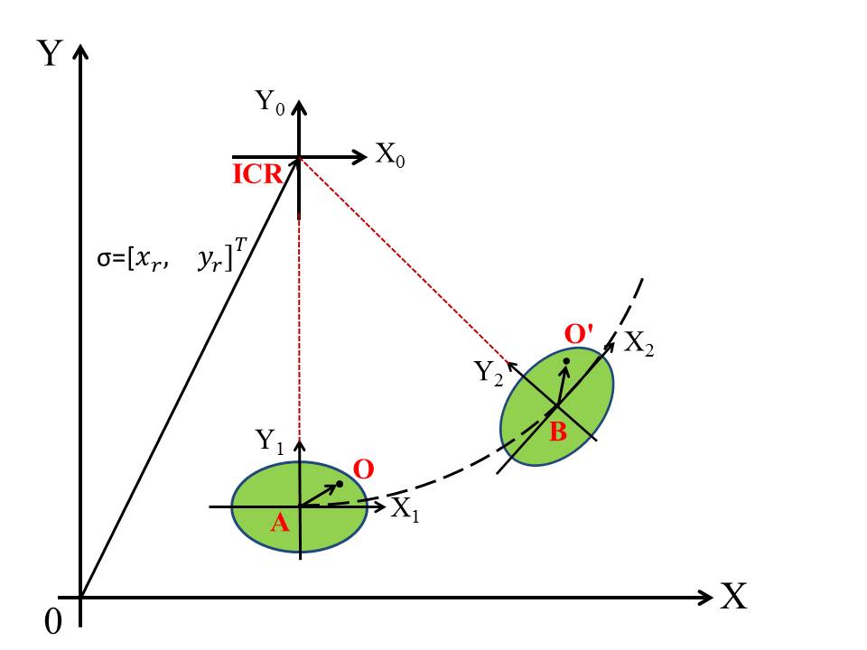
Figure 1: Coordinated turn model of the elliptic extended object.

Substituting (15) into (12), the differential equation of centered moments of ellipse when the object is undergoing coordinated turn motion is given by

$$\dot{\eta}_{ij} =\omega\iint_{R}[\frac{\partial h}{\partial x}(y_{r}-y)+\frac{\partial h}{\partial y}(x-x_{r})]dxdy$$

$$=\omega\iint_{R}[(\frac{\partial h}{\partial y}x-\frac{\partial h}{\partial x}y)+(-\frac{\partial h}{\partial y}x_{r}+\frac{\partial h}{\partial x}y_{r})]dxdy$$ (16)

The dynamic models of the normalized centered moments of the ellipse can be calculated using (16) as

$$\dot{n}_{11}= \omega(n_{20}-n_{02})$$ (17)

$$\dot{n}_{20}= -2\omega n_{11}$$

$$\dot{n}_{02}= 2\omega n_{11}$$

The state space representation of the normalized centered moments of the ellipse $\mathbf{p}_{\mathrm{IM}}=[n_{11},n_{20},n_{02}]^{T}$ are

$$\mathbf{\dot{p}}_{\mathrm{IM}}=\left[\begin{array}[]{ccc}0&\omega&-\omega\\ -2\omega&0&0\\ 2\omega&0&0\end{array}\right]\mathbf{p}_{\mathrm{IM}}$$ (18)

and the solution to the state space in (18) is

$$\mathbf{p}_{\mathrm{\mathrm{IM}}}(t)=\mathbf{M}(t,t_{0})\mathbf{p}_{\mathrm{IM}}(t_{0})$$ (19)

where the transition matrix $\mathbf{M(t,t_{0})}=\left[\begin{smallmatrix}\mathrm{cos}2\theta&\frac{1}{2}\mathrm{sin}2\theta&-\frac{1}{2}\mathrm{sin}2\theta\\ -\mathrm{sin}2\theta&\mathrm{cos}^{2}\theta&\mathrm{sin}^{2}\theta\\ \mathrm{sin}2\theta&\mathrm{sin}^{2}\theta&\mathrm{cos}^{2}\theta\end{smallmatrix}\right]$, where $\theta=\omega\left(t-t_{0}\right)$. The derivation of the transition matrix is shown in the Appendix A.

At each time step $k$, the complete state to be tracked is $\mathbf{p}_{k}=[\begin{array}[]{cc}\mathbf{p}_{\mathrm{IM},k}^{T},&\mathbf{p}_{\mathrm{CT},k}^{T}\end{array}]^{T}$, where $\mathbf{p}_{\mathrm{IM},k}$ is a component of the state corresponding to the image moments, $\mathbf{p}_{\mathrm{CT},k}=[\begin{array}[]{ccccc}x_{c,k},&\dot{x}_{c,k},&y_{c,k},&\dot{y}_{c,k},&\omega_{k}\end{array}]^{T}$ is the vector that includes the position, velocity of the centroid of the extended object and the turning rate of the extended object. The state equation is given as follows

$$\mathbf{p}_{k+1}=\mathbf{F}_{\mathrm{CT}}\mathbf{p}_{k}+\mathbf{\Gamma}\mathbf{w}_{k}$$ (20)

where the state transition matrix $\mathbf{F}_{\mathrm{CT}}=\mathbf{diag}(\mathbf{M},\mathbf{A}),$ $\mathbf{M}=\left[\begin{smallmatrix}\mathrm{cos}2\omega_{k}T&\frac{1}{2}\mathrm{sin}2\omega_{k}T&-\frac{1}{2}\mathrm{sin}2\omega_{k}T\\ -\mathrm{sin}2\omega_{k}T&\mathrm{cos}^{2}\omega_{k}T&\mathrm{sin}^{2}\omega_{k}T\\ \mathrm{sin}2\omega_{k}T&\mathrm{sin}^{2}\omega_{k}T&\mathrm{cos}^{2}\omega_{k}T\end{smallmatrix}\right]$ is obtained from (19), $T$ is a sampling period, $\mathbf{A}=\left[\begin{smallmatrix}1&\frac{\mathrm{sin}\omega_{k}T}{\omega_{k}}&0&-\frac{1-\mathrm{cos}\omega_{k}T}{\omega_{k}}&0\\ 0&\mathrm{cos}\omega_{k}T&0&-\mathrm{sin}\omega_{k}T&0\\ 0&\frac{1-\mathrm{cos}\omega_{k}T}{\omega_{k}}&1&\frac{\mathrm{sin}\omega_{k}T}{\omega_{k}}&0\\ 0&\mathrm{sin}\omega_{k}T&0&\mathrm{cos}\omega_{k}T&0\\ 0&0&0&0&1\end{smallmatrix}\right]$, $\Gamma=\mathbf{diag}(\begin{array}[]{cc}\mathbf{I}_{3\times 3},&\Gamma_{\mathrm{CT}}\end{array})$ with $\Gamma_{\mathrm{CT}}=\left[\begin{smallmatrix}\frac{1}{2}T^{2}&0&0\\ T&0&0\\ 0&\frac{1}{2}T^{2}&0\\ 0&T&0\\ 0&0&T\end{smallmatrix}\right]$, and $\mathbf{w}_{k}\in\mathbb{R}^{6\times 1}$ is the zero-mean Gaussian noise vector. Notice that this model is piece-wise continuous.

II-C Measurement Model

Assuming the uniformly generated measurement $\mathbf{\bar{z}}=[\begin{array}[]{cc}x,&y\end{array}]^{T}$ without the sensor noise, (9) maps the unknown parameters $\mathbf{p}$ to the pseudo-measurement $0$ with the squared scale term $s^{2}\sim\mathcal{U}(0,1)$. The scaling factor $s$ is approximated to be Gaussian distributed with mean $\nicefrac{{2}}{{3}}$ and variance $\nicefrac{{1}}{{18}}$ [12]. Consider the real measurement $\mathbf{z}=[\begin{array}[]{cc}\tilde{x},&\tilde{y}\end{array}]^{T}$ of the unknown true measurement $\mathbf{\bar{z}}=[\begin{array}[]{cc}x,&y\end{array}]^{T}$ in the presence of the additive white Gaussian noise $\boldsymbol{\mathbf{\nu}}=[\nu_{x},\nu_{y}]^{T}$, where $\nu_{x}\sim\mathcal{N}(\begin{array}[]{cc}0,&\sigma_{x}^{2}\end{array})$ and $\nu_{y}\sim\mathcal{N}(\begin{array}[]{cc}0,&\sigma_{y}^{2}\end{array})$, the real measurement $\mathbf{z}$ can be expressed as $\mathbf{z}=\mathbf{\bar{z}}+\mathbf{\boldsymbol{\nu}}$. To find the relationship between the state vector $\mathbf{p}$ and the real measurement $\mathbf{z}=[\begin{array}[]{cc}\tilde{x},&\tilde{y}\end{array}]^{T}$, the measurement model is derived by substituting $\mathbf{z}$ in (9). The following expression can be obtained

$$g(\bar{\mathbf{z}},\mathbf{p})=g(\mathbf{z},\mathbf{p})-f(\mathbf{z},\mathbf{\boldsymbol{\nu},p})=v$$ (21)

where $v$ is the pseudo-measurement with the true value of $0$ and $f(\mathbf{z},\mathbf{\boldsymbol{\nu},p})$ is a polynomial related to the white noise $\mathbf{\boldsymbol{\nu}}$, which has the mean

$$E\left[f(\mathbf{z},\mathbf{\boldsymbol{\nu},p})\right]=\rho(n_{02}\sigma_{x}^{2}+n_{20}\sigma_{y}^{2})$$ (22)

and covariance as

$$C_{f(\mathbf{z},\mathbf{\boldsymbol{\nu},p})} =\rho^{2}\biggl{\{}2n_{02}^{2}\sigma_{x}^{4}+2n_{20}^{2}\sigma_{y}^{4}+4n_{11}^{2}\sigma_{x}^{2}\sigma_{y}^{2}$$ (23)

$$+4\left[n_{02}(\widetilde{x}-x_{g})-n_{11}(\widetilde{y}-y_{g})\right]^{2}\sigma_{x}^{2}$$

$$+4\left[n_{20}(\widetilde{y}-y_{g})-n_{11}(\widetilde{x}-x_{g})\right]^{2}\sigma_{y}^{2}\biggr{\}}$$

where $\rho=\nicefrac{{1}}{{4\left(n_{20}n_{02}-n_{11}^{2}\right)}}$. The derivation of $f(\mathbf{z},\mathbf{\boldsymbol{\nu},p})$ and its first two moments are shown in the Appendix B. Since the measurement model is highly nonlinear, the UKF presented in next section, is used to estimate the state vector $\mathbf{p}$.

III UKF for Extended Object Tracking using Image Moments Based RHM

On the basis of the dynamic motion models and the measurement model, a recursive Bayesian state estimator for tracking the elliptic extended objects is derived. The state vector of the elliptic extended object is $\mathbf{p}$. At each time step, several measurement points from the volume or area of the object’s extent are received. The task of the Bayesian state estimator is to perform backward inference, inferring the true state parameters from the measurement points. The measurement points at time step $k$ is denoted as $\mathbf{Z}_{k}=\{\mathbf{z}_{k,l}\}_{l=1}^{L_{k}}$, assuming there are $L_{k}$ measurements at time $k$ and each measurement point is $\mathbf{z}_{k,l}=[\begin{array}[]{cc}x,&y\end{array}]^{T}$. The state vector up to time step $k$ when all the measurements are incorporated is denoted as $\mathbf{p}_{k}$. Suppose that the posterior probability density function (pdf) $p(\mathbf{p}_{k-1}\mid\mathbf{Z}_{k-1})$ at time step $k-1$ is available, the prediction $p(\mathbf{p}_{k}\mid\mathbf{Z}_{k-1})$ for time step $k$ is given by the Chapman-Kolmogorov equation as [36]

$$p(\mathbf{p}_{k}\mid\mathbf{Z}_{k-1})=\int p(\mathbf{p}_{k}\mid\mathbf{p}_{k-1})p(\mathbf{p}_{k-1}\mid\mathbf{Z}_{k-1})d\mathbf{p}_{k-1}$$ (24)

the state vector evolves by the conditional density function $p(\mathbf{p}_{k}\mid\mathbf{p}_{k-1})$. Assuming the Markov model is conformed, the conditional density function $p(\mathbf{p}_{k}\mid\mathbf{p}_{k-1})$ can be derived based on different dynamic models in Subsection II-B. Assuming the measurements $\mathbf{Z}_{k}=\{\mathbf{z}_{k,l}\}_{l=1}^{L_{k}}$ at time $k$ are independent, the prediction $p(\mathbf{p}_{k}\mid\mathbf{z}_{k,l})$ is updated recursively via Bayes rule as

$$p(\mathbf{p}_{k}\mid\mathbf{z}_{k,l})\wasypropto p(\mathbf{z}_{k,l}\mid\mathbf{p}_{k})p(\mathbf{p}_{k}\mid\mathbf{z}_{k,l-1})$$ (25)

where $p(\mathbf{p}_{k}\mid\mathbf{z}_{k,0})=p(\mathbf{p}_{k}\mid\mathbf{Z}_{k-1})$ and $p(\mathbf{p}_{k}\mid\mathbf{Z}_{k})=p(\mathbf{p}_{k}\mid\mathbf{z}_{k,L_{k}})$.

When the target is moving with uniform motion (constant velocity model, which is a linear system), its states $\mathbf{p}_{k|k-1}$ and covariance $C_{k|k-1}$ are predicted based on the dynamic model (14) as

$$\mathbf{p}_{k|k-1} =\mathbf{F}_{\mathrm{CV}}\mathbf{p}_{k}$$ (26)

$$C_{k|k-1} =\mathbf{F}_{\mathrm{CV}}\mathbf{p}_{k}\mathbf{F}_{\mathrm{CV}}^{T}+\mathbf{C}_{\mathrm{CV}}$$ (27)

However, the proposed image moments based RHM and its dynamic model such as coordinated turn model are nonlinear. When the system is nonlinear, the linearization method like the extended Kalman filter (EKF) will introduce large errors in the true posterior mean and covariance. UKF addresses this problem by the method of unscented transformation (UT), which doesn’t require the calculations of the Jacobian and Hessian matrices. The UT sigma point selection scheme results in approximations that are accurate to the third order for Gaussian inputs for all nonlinearities and has the same order of the overall number of computations as the EKF [37]. When the state variables in $\mathbf{p}\in\mathbb{R}^{M\times 1}$ with mean $\mathbf{\bar{p}}$ and covariance $C_{\mathbf{p}}$ are propagating through a nonlinear function $\mathbf{y}=f(\mathbf{p})$, such as (19) or (21), the mean $\bar{\mathbf{y}}$ and covariance $C_{\mathbf{y}}$ of $\mathbf{y}$ are approximated by generating the UT sigma points $\mathcal{X}_{i}$ as [37]

$$\bar{\mathbf{y}} =\sum_{i=0}^{2M}W_{i}^{(m)}\mathcal{Y}_{i}$$ (28)

$$C_{\mathbf{y}} =\sum_{i=0}^{2M}W_{i}^{(C)}\left\{\mathcal{Y}_{i}-\bar{\mathbf{y}}\right\}\left\{\mathcal{Y}_{i}-\bar{\mathbf{y}}\right\}$$ (29)

where $\mathcal{Y}_{i}=f(\mathbf{\mathcal{X}}_{i})$. The sigma points $\mathcal{X}_{i}$ and the weights $W_{i}^{(m)}$ and $W_{i}^{(C)}$ are calculated by [37]

$$\mathcal{X}_{0} =\mathbf{\bar{p}}$$ (30)

$$\mathcal{X}_{i} =\mathbf{\bar{p}}+\left(\sqrt{(M+\lambda)C_{\mathbf{p}}}\right)_{i} i=1,\ldots,M$$

$$\mathcal{X}_{i} =\mathbf{\bar{p}}-\left(\sqrt{(M+\lambda)C_{\mathbf{p}}}\right)_{i} i=M+1,\ldots 2M$$

$$W_{0}^{(m)} =\lambda/(M+\lambda)$$

$$W_{0}^{(C)} =\lambda/(M+\lambda)+(1-\alpha^{2}+\beta)$$

$$W_{i}^{(m)} =W_{i}^{(C)}=1/\left[2(M+\lambda)\right] i=1,\ldots,2M$$

where $\lambda$ is the scaling parameter as $\lambda=\alpha^{2}(M+\kappa)-M$, $\alpha$ is the parameter determines the spread of the sigma points around the mean $\bar{\mathbf{p}}$, $\kappa$ is the secondary scaling parameter usually set to $0$ and $\beta$ is the parameter to incorporate the prior knowledge of the distribution of $\mathbf{p}$. The UKF for image moments based random hypersurface model is illustrated in Algorithm. 1.

Set the time steps ${N}$;

Set the initial state vector $\mathbf{p}_{0}$ and covariance $C_{0}$ ;

for $k$=1 to N do

      

      case Constant velocity model do

            

            State $\mathbf{p}_{k|k-1}$ is predicted as in (26);

            Covariance $C_{k|k-1}$ is predicted as in (27);

      

      case Coordinated turn model do

            

            Augment the state vector $\mathbf{p}_{k-1}^{a}=\left[\left(\mathbf{p}_{k-1}\right)^{T},\mathbf{w}_{k}^{T}\right]^{T}$;

            Calculate sigma points using (30);

            States prediction based on (20) with sigma points;

            Using (28), (29) to calculate the mean and covariance of the state vector $\mathbf{p}_{k|k-1}$;

      

      Obtain the measurement points $\mathbf{Z}_{k}=\{\mathbf{z}_{k,l}\}_{l=1}^{L_{k}}$ at time step $k$;

      

      for $l$=1 to $L_{k}$ do

            

            Calculate the mean and covariance of $f(\mathbf{z}_{k,l},\mathrm{\mathrm{\mathbf{\boldsymbol{\nu}}}},\mathbf{p}_{k|k-1})$ using (22) and (23);

            

            Augment the state vector $\mathbf{p}_{k|k-1,l}^{a}=\left[\left(\mathbf{p}_{k|k-1,l}\right)^{T},f(\mathbf{z}_{k,l},\mathrm{\mathrm{\mathbf{\boldsymbol{\nu}}}},\mathbf{p}_{k|k-1}),s\right]^{T}$;

            

            Calculate sigma points using (30);

            

            Pseudo-measurement $v_{k,l}$ calculated based on (21) for measurement point $\mathbf{z}_{k,l}$;

            

            Using (28), (29) to calculate the mean and covariance of the $v_{k,l}$;

            

            Update state vector $\mathbf{p}_{k,l}$;

            

      

Algorithm 1 UKF with sequential processing of measurements.

IV Tracking extended target with IMM

The proposed image moments based random hypersurface model is embedded with the IMM approach for tracking extended target undergoing complex trajectories in this section. When the extended target is switching between maneuvering and non-maneuvering behaviors, its kinematic state and spatial extent may change abruptly. Multiple model approaches, such as interacting multiple model (IMM), are effective to track the target with complex trajectories, especially with high maneuvering index (larger than $0.5$) [34, 33, 35]. The IMM approach assumes the target obeys one of a finite number of motion models and identifies the beginning and the end of the motion models by updating the model probabilities. The adaptation via model probability update helps the IMM approach keep the estimation errors consistently low, both during maneuvers as well as no-maneuver intervals. Details about the IMM for point target tracking can be found in literature such as [33].

The proposed image moments based random hypersurface model with the dynamic motion models, such as the constant velocity motion model and the coordinated turn motion model in Section II, are integrated in an IMM framework. Since the dynamic motion model and the measurement model are nonlinear, the UKF-IMM algorithm is proposed. The flowchart of the UKF-IMM algorithm are shown in Fig. 2, where $\mu_{k-1}^{i|j}$ is the mixing probability, $p_{i|j}$ is the Markov chain transition matrix between the $i\mathrm{th}$ and $j\mathrm{th}$ models and $\Lambda_{k}^{j}$ are likelihood function corresponding to the $j\mathrm{th}$ model. There are multiple measurement points at each time step, the sequential approach is adopted for UKF and the likelihood function is generated based on the measurement model.

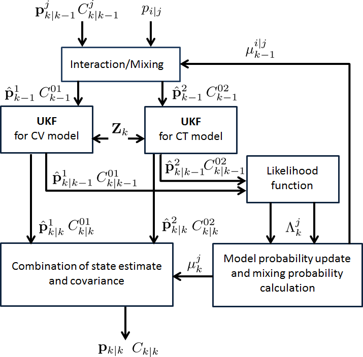
Figure 2: Flowchart of UKF-IMM framework.

At each time step, assuming there are $L_{k}$ measurements $\mathbf{Z}_{k}=\{\mathbf{z}_{k,l}\}_{l=1}^{L_{k}}$. The pseudo-measurement variable $v_{k,l}$ can be generated for each measurement $\mathbf{z}_{k,l}$, based on the predicted state vector $\mathbf{p}_{k|k-1}^{j}$, covariance $C_{k|k-1}^{j}$ and the measurement model in (21). The mean and the covariance of the pseudo-measurement variable $v_{k,l}$, can be obtained by the method of unscented transformation (UT). Assuming the measurements $\mathbf{Z}_{k}=\{\mathbf{z}_{k,l}\}_{l=1}^{L_{k}}$ are independent identically Gaussian distributed, the log-likelihood function based on the pseudo-measurement variable $v_{k,l}$ is

$$\log\Lambda_{k}^{j}=\sum_{l=1}^{L_{k}}\left[-\frac{(0-\mu_{v,l})^{2}}{2\sigma_{v,l}^{2}}-\log\left(\sqrt{2\pi\sigma_{v,l}^{2}}\right)\right]$$ (31)

where $\mu_{v,l}$ and $\sigma_{v,l}^{2}$ are the mean and covariance of the pseudo-measurement $v_{k,l}$, generated for each measurement point $\mathbf{z}_{k,l}$. In many cases, the likelihood $\Lambda^{j}\left(k\right)$ can become extremely small. To avoid this issue, the average log-likelihood $\log\bar{\Lambda}^{j}\left(k\right)$ is used which is given by

$$\log\bar{\Lambda}_{k}^{j}=\frac{1}{n_{k}}\log\Lambda_{k}^{j}$$ (32)

and

$$\bar{\Lambda}_{k}^{j}=\exp\left(\log\bar{\Lambda}_{k}^{j}\right)$$ (33)

which is the value of the measurement likelihood between $0$ and $1$. This measurement likelihood is used in the IMM filter. The details of the calculation of the measurement likelihood is show in Algorithm 2.

Obtain the predicted state vector $\mathbf{p}_{k|k-1}^{j}$ and covariance $C_{k|k-1}^{j}$ of model $j$;

Obtain the measurement points $\mathbf{Z}_{k}=\{\mathbf{z}_{k,l}\}_{l=1}^{L_{k}}$ at time step $k$;

for $l$=1 to $L_{k}$ do

      

      Calculate the mean and covariance of $f(\mathbf{z}_{k,l},\mathrm{\mathrm{\mathbf{\boldsymbol{\nu}}}},\mathbf{p}_{k|k-1})$ using (22) and (23);

      

      Augment the state vector $\mathbf{p}_{k|k-1,l}^{a}=\left[\left(\mathbf{p}_{k|k-1,l}^{j}\right)^{T},f(\mathbf{z}_{k,l},\mathrm{\mathbf{\boldsymbol{\nu}}},\mathbf{p}_{k|k-1}),s\right]^{T}$;

      

      Calculate sigma points $\mathcal{X}$ using (30);

      

      Propagate sigma points $\mathcal{X}$ through the measurement model in (21);

      

      Using (28), (29) to calculate the mean and covariance of the pseudo-measurement $v_{k,l}$;

      

      Summation of the value of the log-likelihood function using (31);

      

Calculation of the value of the average log-likelihood function using (32) and the measurement likelihood using (33);

Algorithm 2 Calculation of the measurement likelihood $\bar{\Lambda}_{k}^{j}$ corresponding to the $j\mathrm{th}$ model by unscented transformation.

V Simulation Results

In this section, several simulation tests are conducted to evaluate the performance of the proposed image moments based extended object tracking. To validate the measurement model in (21), the shapes of the static objects are estimated with different noise levels in the first simulation. Then the tracking of the extended target moving with linear motion and coordinated turn motion are demonstrated. The constant velocity model in (14) and the nearly coordinated turn model in (20) are used and validated for these cases. Two targets with the shapes of the plus-sign and ellipse are used in the simulations. At last, tracking of targets moving with maneuvering and non-maneuvering intervals are presented. Two scenarios are simulated in this test. One with slow motion and maneuvers and the other with fast motion and maneuvers. The UKF-IMM algorithm with constant velocity model and the nearly coordinated turn model is applied in these cases. The RMM and its combination with the IMM in [20] are implemented as a benchmark comparison for our proposed image moments based random hypersurface model.

The intersection over union (IoU) is used as the metric to evaluate the proposed algorithm. The IoU is defined as the area of the intersection of the estimated shape and the true shape divided by the union of the two shapes[38]

$$\mathbf{IoU}=\frac{area(\mathbf{p})\cap area(\mathbf{\hat{p}})}{area(\mathbf{p})\cup area(\mathbf{\hat{p}})}$$ (34)

where $\mathbf{p}$ is the true state vector and $\mathbf{\hat{p}}$ is the estimated state vector. $\mathbf{IoU}$ is between $0$ and $1$, where the value $1$ corresponds to a perfect match between the estimated area and the ground-truth. Additionally, the root mean squared errors (RMSE) of the estimated position and velocity of the centroid $(x_{c,}y_{c})$ of the extended target are also evaluated, which are defined as

$$\mathbf{RMSE}=\sqrt{\frac{1}{N}\sum_{i=1}^{N}\xi_{i}^{2}}$$ (35)

where $N$ is the Monte Carlo runs, $\xi_{i}$ is the error of the estimation from the $i$th run. For the RMSE of the position, $\xi_{i,p}\triangleq(\hat{x}_{c}-x_{c})^{2}+(\hat{y}_{c}-y_{c})^{2}$, where $(\hat{x}_{c,}\hat{y}_{c})$ is the estimated centroid of the extended target and $(x_{c,}y_{c})$ is the ground-truth. Similarly, for the RMSE of the velocity, the estimation error is defined as $\xi_{i,v}\triangleq(\hat{\dot{x}}_{c}-\dot{x}_{c})^{2}+(\hat{\dot{y}}_{c}-\dot{y}_{c})^{2}$, where $(\hat{\dot{x}}_{c,}\hat{\dot{y}}_{c})$ is the estimated velocity of the centroid and $(\dot{x}_{c,}\dot{y}_{c})$ is the ground-truth.

V-A Static Extended Objects

The plus-sign shaped target is made up of two rectangles with the width and height of $3\mathrm{cm}$ and $0.5\mathrm{cm}$, and $0.5\mathrm{cm}$ and $2\mathrm{cm}$, respectively. The major and minor axes of the elliptic target are set to $3\mathrm{cm}$ and $2\mathrm{cm}$, respectively. The simulation is performed by uniformly sampling $400$ points from the static extended objects. Three different levels of additive Gaussian white noises with variances such as $\mathbf{diag}(\begin{array}[]{cc}0.1^{2},&0.1^{2}\end{array})$ (low), $\mathbf{diag}(\begin{array}[]{cc}0.5^{2},&0.5^{2}\end{array})$ (medium) and $\mathbf{diag}(\begin{array}[]{cc}1,&1\end{array})$ (high) are used to generate the noisy measurements.

UFK is used for estimating the state given noisy measurements of points uniformly sampled from the plus-sign-shaped and ellipse-shaped extended objects. The state is initialized as a circle with radius of $0.89\mathrm{cm}$ located at the origin. The estimation results for the plus-sign-shaped object are shown in Figs. 3(a), 3(b), 3(c) and the estimation results for the ellipse-shaped object are shown in Figs. 3(d), 3(e), 3(f). The mean values of the IoU of the static ellipse and the plus-sign-shaped targets with $3$ different noise levels are shown in Table I. The image moments based measurement model can precisely estimate the shape of the targets. With the increases in covariance of the measurement noise, the proposed image moments based model also gives a shape close to the actual shape of the targets. The IoU value for the plus-sign shaped target is lower than the elliptical target because the ellipse is used to roughly estimate the plus-sign shape.

    

    

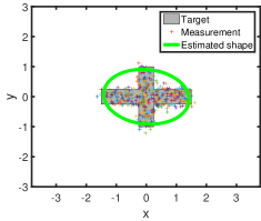
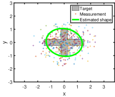
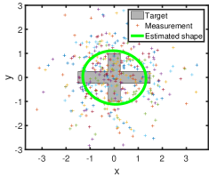
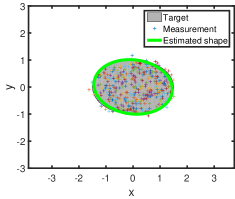
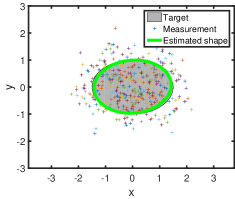
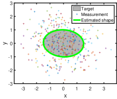
Figure 3: Estimation of the shape of extended targets with different measurement noise levels in a particular run; estimation of the shape is drawn in green color and the gray shape is the ground truth. (a) - (c) estimations of the shape of the extended target (with the shape of the plus-sign) with three different measurement noise levels; (d) - (f) estimations of the elliptic target with three different measurement noise levels.

Table I: The mean value of Intersection-Over-Union (IoU) between the true and the estimated target region in different simulated scenarios. Three noise levels (low , medium and high) are used to evaluate the static targets (ellipse and plus-sign-shaped target). The mean value is calculated over 100 Monte Carlo runs.

Target shape	Static target			Linear motion	Coordinated turn motion
	Low	Medium	High
Ellipse	$0.90$	0.88	0.85	0.88	0.87
Plus-sign	$0.48$	0.48	0.47	0.46	0.48

         

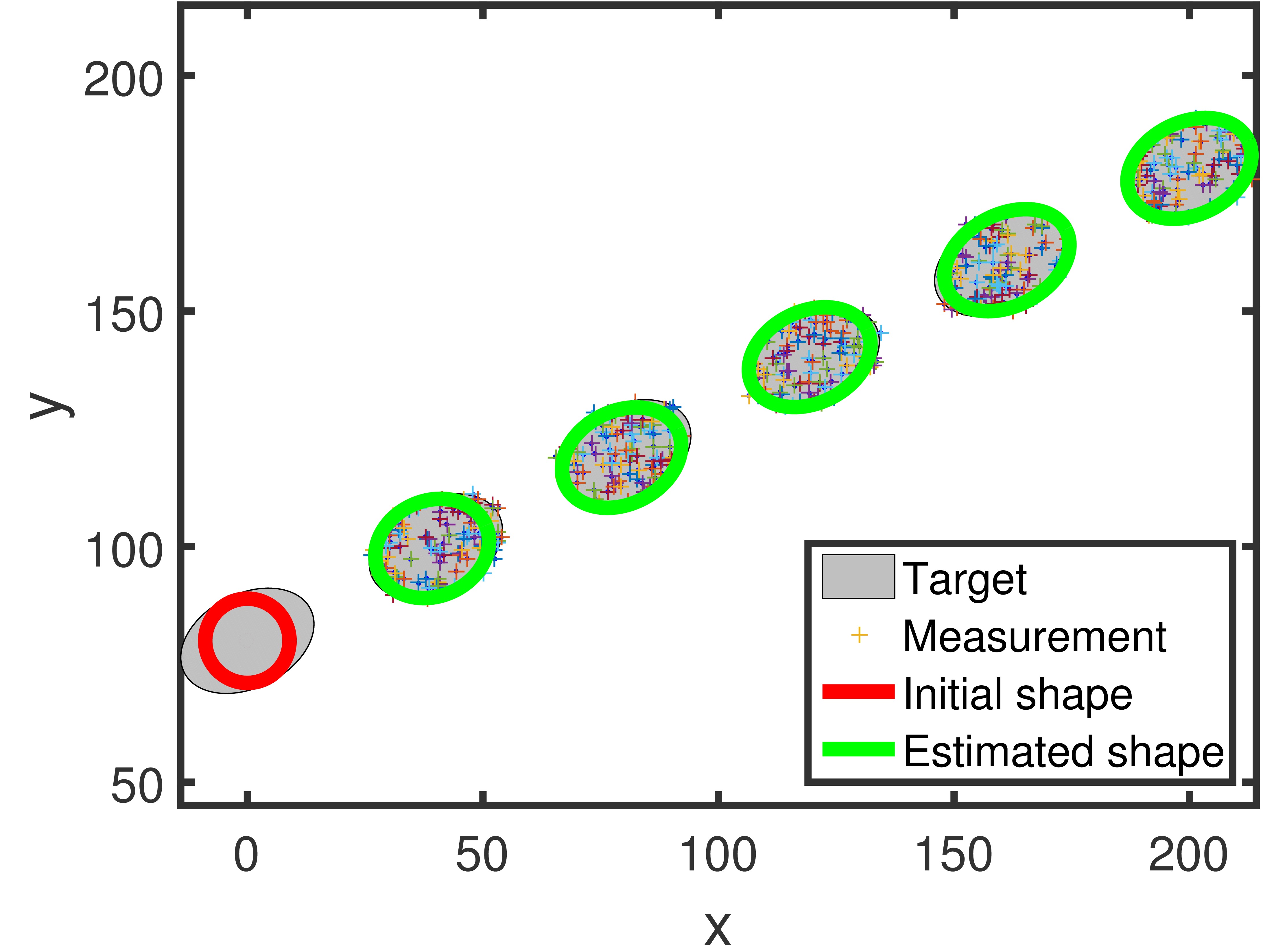
(a) ellipse

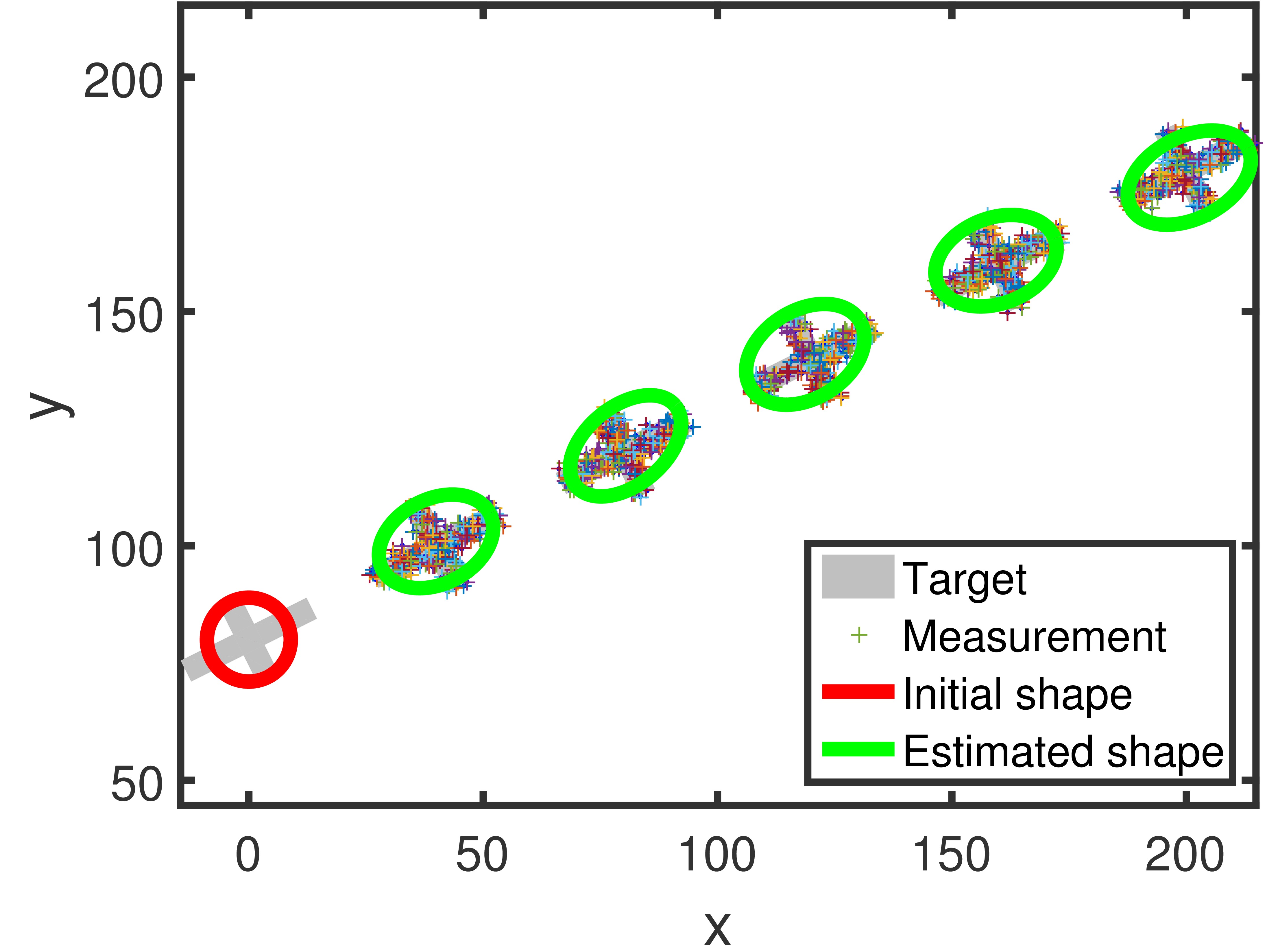
(b) plus-sign

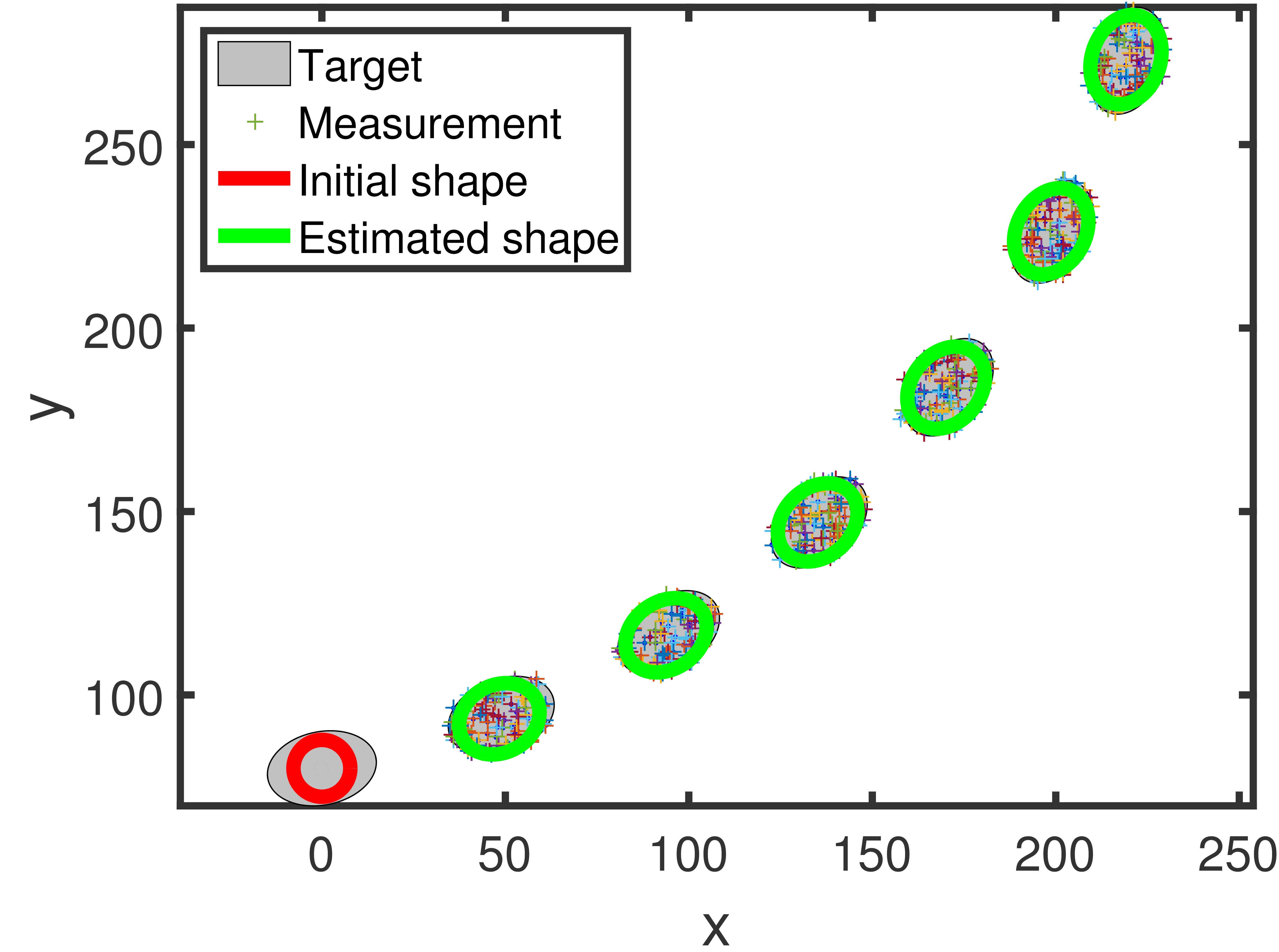
(c) ellipse

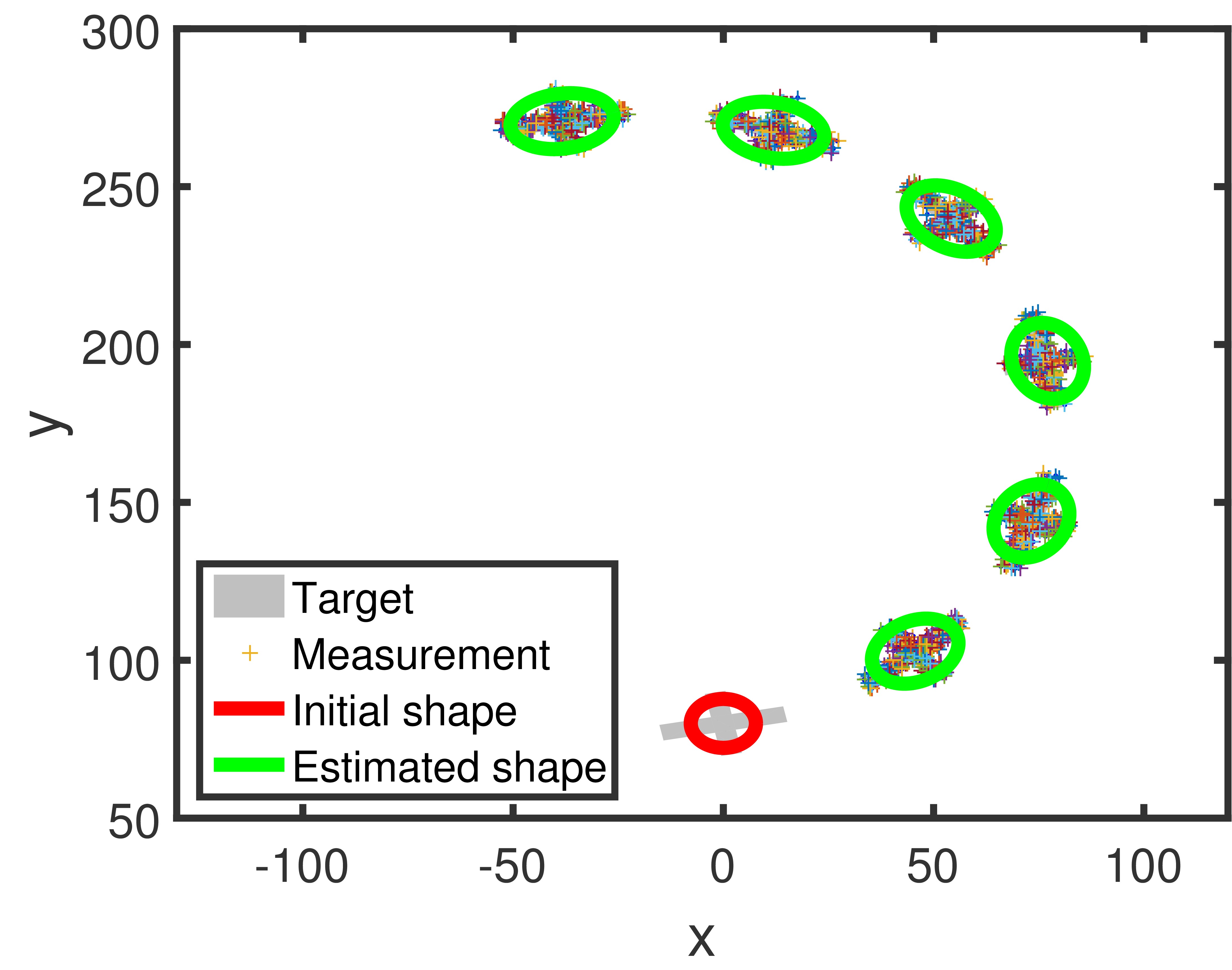
(d) plus-sign

Figure 4: Tracking of the extended objects during constant velocity model or coordinated turn model in a particular run; Initial shape is shown in red color, estimation of the shape is drawn in green color and the gray shape is the ground truth; (a) ellipse with a constant velocity; (b) plus-sign with a constant velocity; (c) the ellipse executes a $1^{\circ}/s$ coordinated turn; (d) the plus-sign executes a $3^{\circ}/s$ coordinated turn.

V-B Linear Motion

In this subsection, extended objects with plus-sign and elliptical shapes moving with a constant velocity are simulated. The plus-sign shaped target is made up of two rectangles with the width and height of $30\mathrm{cm}$ and $5\mathrm{cm}$, and $5\mathrm{cm}$ and $20\mathrm{cm}$, respectively. For the ellipse-shaped object, the major and minor axes are set to $30\mathrm{cm}$ and $20\mathrm{cm}$, respectively. The extended objects start moving from position $[\begin{array}[]{cc}0,&80\end{array}]^{T}$$\mathrm{cm}$ with a constant velocity of $[\begin{array}[]{cc}4,&2\end{array}]^{T}$$\nicefrac{\mathrm{cm}}{\mathrm{s}}$ for $60$ seconds and the measurements are generated from the targets at every $10$ seconds. At each time step $k$, $100$ measurement points uniformly sampled from the objects are generated.

For UKF implementation, the states are initialized as a circle with radius of $8.9\mathrm{cm}$, located at $[\begin{array}[]{cc}0,&80\end{array}]^{T}$$\mathrm{cm}$ with a constant velocity of $[\begin{array}[]{cc}4,&2\end{array}]^{T}$$\nicefrac{\mathrm{cm}}{\mathrm{s}}$. The Gaussian white noise variance is selected as $\mathbf{diag}(\begin{array}[]{cc}1&1\end{array})$ for each point measurement. The parameter $q$ for the process noise covariance in the constant velocity model in (14) is set as $q=0.2$ and $\mathbf{C}_{\mathrm{IM}}=\mathrm{\mathbf{diag}}(0.1,0.1,0.1)$. The tracking results for ellipse-shaped extended object are shown in Fig. 4(a) and for plus-sign-shaped extended object are shown in Fig. 4(b). It can be seen that the shapes of targets are being estimated accurately as more measurements are obtained. The mean value of the RMSE of the position over $100$ Monte Carlo runs is $0.58\mathrm{cm}$ for ellipse and $1.29\mathrm{cm}$ for the plus-sign. The mean value of the RMSE of the velocity over $100$ Monte Carlo runs is $0.50\nicefrac{\mathrm{cm}}{\mathrm{s}}$ for ellipse and $0.25\nicefrac{\mathrm{cm}}{\mathrm{s}}$ for the plus-sign. The mean values of the IoU of the ellipse and the plus-sign-shaped targets during the linear motion are shown in Table I.

V-C Coordinated Turn Motion

The extended object undergoing coordinated turn is simulated in this case. The extended object with the shape of the plus-sign starts from $\left[\begin{array}[]{cc}0,&80\end{array}\right]^{T}\mathrm{cm}$ with velocity $\left[\begin{array}[]{cc}5,&1\end{array}\right]^{T}\nicefrac{\mathrm{cm}}{\mathrm{s}}$ at time $t=0$, then it executes a $1^{\circ}/s$ coordinated turn for $60$ seconds. The extended elliptic object executes a $3^{\circ}/s$ coordinated turn for $60$ seconds. The sampling interval is $10$ seconds. At each time step, $100$ noisy measurement points are uniformly generated from the extents of the targets. The noise variance is selected as $\mathbf{diag}(\begin{array}[]{cc}1,&1\end{array})$ for each point measurement.

The extended objects executing a coordinated turn are estimated based on the dynamic model (20). The states are initialized as a circular shape with radius of $7.8\mathrm{cm}$. The tracking results for ellipse-shaped object are shown in Fig. 4(c) and tracking results for plus-sign-shaped object are shown in Fig. 4(d). The mean value of the RMSE of the position over $100$ Monte Carlo runs is $0.81\mathrm{cm}$ for ellipse and $0.96\mathrm{cm}$ for the plus-sign. The mean value of the RMSE of the velocity over $100$ Monte Carlo runs is $0.45\nicefrac{\mathrm{cm}}{\mathrm{s}}$ for ellipse and $0.32\nicefrac{\mathrm{cm}}{\mathrm{s}}$ for the plus-sign. The mean values of the IoU of the ellipse and the plus-sign-shaped targets during the coordinated turn motion are shown in Table I. The image moments based model, which provides a dynamic model for the shape of extended object undergoing a coordinated turn, can estimate the positions and velocities of the target, as well as the orientations and extents of the targets very accurately.

V-D Complex trajectories

The image moments based RHM is embedded in the IMM framework. The proposed model is tested in two simulations of the extended elliptical objects switching between maneuvering and non-maneuvering intervals multiple times.

V-D1 Slow motion and maneuvering case

The target is moving with a constant velocity of $50\nicefrac{\mathrm{km}}{\mathrm{h}}$, with initial state in Cartesian coordinates $\mathbf{p}_{0}=\left[x_{c},\dot{x}_{c},y_{c},\dot{y}_{c}\right]^{T}=[0,9.8,0,-9.8]^{T}$(with position in m). The target first executes a $45^{\circ}$ coordinated turn with the turning rate of $0.46\nicefrac{{\circ}}{{s}}$ at 260 second for 100 seconds, then it goes through two $90^{\circ}$ coordinated turns with the turning rate of $0.90\nicefrac{{\circ}}{{s}}$ at 570 second and 830 second for $100$ seconds. The trajectory is shown in Fig. 5. The major and minor axes of the elliptical target are set to $340$m and $80$m, respectively. The number of the measurements in each scan is generated based on the Poisson distribution with mean of $10$, and the measurement points are uniformly distributed. The variance of the measurement noise is $\mathbf{diag}(\begin{array}[]{cc}10^{2},&10^{2}\end{array})$, and the sampling time is $10$s.

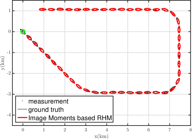
Figure 5: The trajectory, measurements and one example run of the simulation. Estimation results are shown for every $30$ seconds.

      

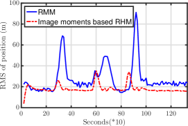
(a) Average RMSE of position

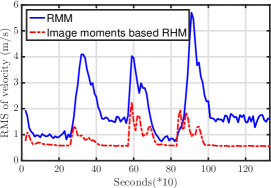
(b) Average RMSE of velocity

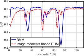
(c) Average IoU

Figure 6: Simulation results of the proposed image moments based RHM algorithm compared with the RMM algorithm in [20] over $1000$ Monte Carlo runs: (a) The average RMSE of the position of the centroid; (b) The average RMSE of the velocity of the centroid; (c) The average IoU.

The proposed Image moments based random hypersurface model with UKF-IMM algorithm is compared with the RMM with IMM algorithm in [20]. The RMM-IMM algorithm uses two models. The model with a high kinematic process noise and a high extension agility accounts for abrupt changes in shape and orientation during maneuvers, and another model with low kinematic noise and a low extension agility accounts for the non-maneuvers. The extension agility is set as 10 and 5 separately for both models. The kinematic states of both models use the constant velocity model (the kinematic dynamic model in (14)), and the parameter $q$ in (14) is set as $10$ and $0.1$ respectively. The proposed image moments based RHM with the UKF-IMM filter combines the constant velocity model in (14) and the coordinated turn model in (20). The parameter $q$ for the process noise covariance in the constant velocity model in (14) is set as $0.01$ and $\mathbf{C}_{\mathrm{IM}}=\mathrm{\mathbf{diag}}(1,1,1)$. For the coordinated turn model in (20), $\mathbf{w}_{k}=[0.01,0.01,0.01,0.0001,0.0001,\left(0.02\times\pi/180\right)^{2}]^{T}$. The initial probability $\mu_{0}^{j}$ of the two models in the IMM filter for both algorithms is set as equal and the Markov chain transition matrix is selected to be $p_{i|j}=\left[\begin{smallmatrix}0.90&0.10\\ 0.25&0.75\end{smallmatrix}\right]$. The model probability of the proposed algorithm is shown in Fig. 7. With the same trajectory, the two algorithms run with 1000 Monte Carlo runs and their simulation results are shown in Fig. 6. The proposed algorithm has lower RMS errors both for position and velocity and the RMM algorithm in [20] has better IOU values.

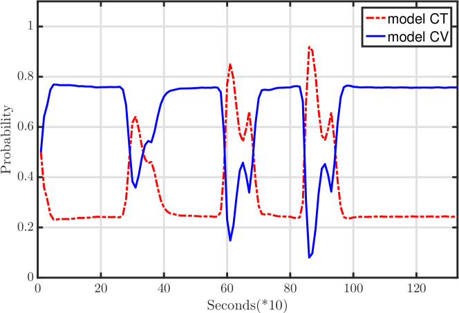
Figure 7: Model probability of the UKF-IMM filter for the image moments based RHM.

V-D2 Fast motion and maneuvering case

The typical trajectory from [33] is used for this simulation and shown in Fig. 8. The target is moving with a constant velocity of $250\nicefrac{\mathrm{m}}{\mathrm{s}}$, with initial state in Cartesian coordinates $\mathbf{p}_{0}=\left[x_{c},\dot{x}_{c},y_{c},\dot{y}_{c}\right]^{T}=[0,0,0,250]^{T}$(with position in m). The details of its maneuvering and non-maneuvering intervals are shown in Table II. For easily visualizing, the major and minor axes of the elliptical target are enlarged to $300$m and $150$m, respectively. The number of the measurements in each scan is generated based on the Poisson distribution with mean of $50$, and the measurement points are uniformly distributed. The variance of the sensor noise is $\mathbf{diag}(\begin{array}[]{cc}3^{2},&3^{2}\end{array})$, and the sampling time is $10$s.

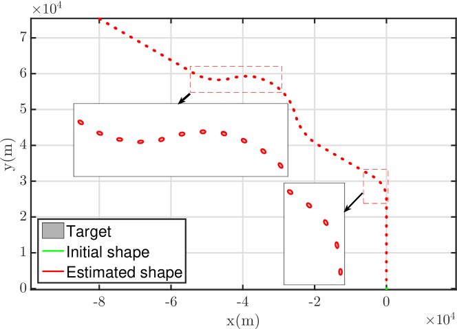
Figure 8: Trajectory of the extended object and the estimation results of the image moments based RHM in one run.

Table II: Details on the complex trajectory.

Time (second)	Model	Turning rate (${}^{\circ}/s$)	Turning direction	Acceleration
$0-100$	CV	0	$-$	$-$
$100-130$	CT	2	left	0.89g
$130-200$	CV	0	$-$	$-$
$200-245$	CT	1	right	0.45g
$245-335$	CT	1	left	0.45g
$335-380$	CT	1	right	0.45g
$380-500$	CV	0	$-$	$-$

The RMM-IMM algorithm [20] also consists of two models. The extension agility is set as 10 and 5 separately for both models. The kinematic states of both models use the constant velocity model (the kinematic dynamic model in (14)), and the parameter $q$ in (14) is set as $100$ and $0.3$ separately. The proposed image moments based RHM with the UKF-IMM filter combines the constant velocity model in (14) and the coordinated turn model in (20). The parameter $q$ for the process noise covariance in the constant velocity model in (14) is set as $0.05$ and $\mathbf{C}_{\mathrm{IM}}=\mathrm{\mathbf{diag}}(50000,50000,50000)$. For the coordinated turn model in (20), $\mathbf{w}_{k}=[1000,1000,1000,0.5,0.5,\left(0.05\times\pi/180\right)^{2}]^{T}$. The initial probability $\mu_{0}^{j}$ of the two models in the IMM filter for both algorithms is set as equal and the Markov chain transition matrix is selected to be $p_{i|j}=\left[\begin{smallmatrix}0.85&0.15\\ 0.90&0.10\end{smallmatrix}\right]$. The model probability of the proposed algorithm is shown in Fig. 10. With the same trajectory, the two algorithms run with 1000 Monte Carlo runs and their simulation results are shown in Fig. 9.

      

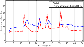
(a) Average RMSE of position

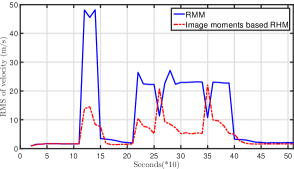
(b) Average RMSE of velocity

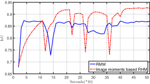
(c) Average IoU

Figure 9: Comparison of the estimation results of the image moments based RHM and the RMM algorithm developed in [20].

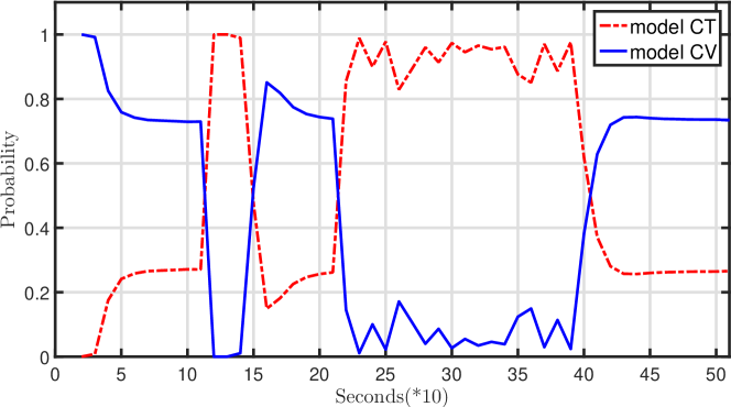
Figure 10: Average model probabilities in $1000$ runs.

The proposed image moments based RHM and its measurement and dynamic models are validated in the simulations of the static targets, the targets with linear motion and with the coordinated turn motion. As the noise levels are increased, the size of the estimated elliptical shape doesn’t increase as the sensor noise increases. When the targets are performing during the linear motion or the coordinated turn motion, the proposed algorithm can predict the position and velocity of the moving target, as well as the spatial extent and orientation of the targets. To estimate the target moves switching between the maneuvering and non-maneuvering intervals. the proposed image moments based RHM is embedded with the IMM framework. The proposed average measurement log-likelihood function can estimate the model probability accurately and consistently. The RMSE values of the position and velocity of the target’s centroid is lower than the results from the RMM. The state variables of the RMM is the centroid and the random matrix, which is updated based on the mean and spread matrix of the measurement points[20]. The proposed RHM using the centroid and the three image moments as the state variables, which is updated based on each individual measurement point. When the number of the measurement points is small or noisy, the proposed image moments based RHM estimates the position and velocity of the centroid accurately, while the mean of the measurement points is far away from the position of the centroid. The accurate dynamic model has the advantage of predicting the location of the target, especially when predict the location of the target undergoing fast motion and the sampling frequency is relatively low.

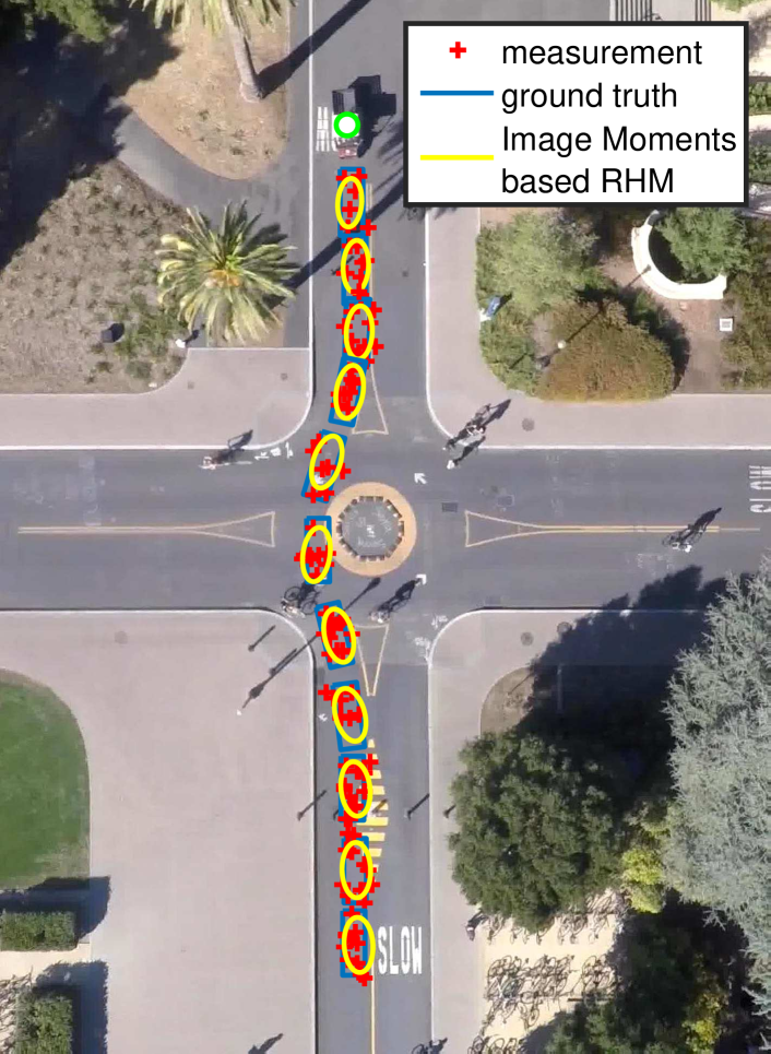
Figure 11: Illustration of the estimation results in a particular run by the proposed image moments based RHM; The target is at first estimated as the circle ( green circle ) with the radius of 20 pixels; The estimated results (yellow ellipse), the measurements (red crossing) and the ground truth (blue box) are shown for every 40 frames.

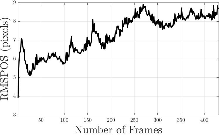
(a) Average RMSE of the position

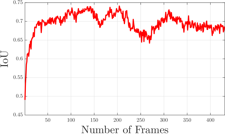
(b) Average IoU

Figure 12: Tracking results of the proposed image moments based RHM algorithm over $1000$ Monte Carlo runs.

VI Experiment

In this section, the proposed image moments based RHM is applied for tracking a moving car represented as an extended object in a real video. A short video clip from the Stanford drone dataset [39] is used, which shows a moving car from a bird’s eye view. The video is captured with a 4k camera mounted on a quadcopter platform (a 3DR solo) hovering above an intersection on a university campus at an altitude of approximately $80$ meters which contains 431 frames with the image size of 1422 by 1945 pixels and the video has been undistorted and stabilized [39]. The ground truth is manually labeled at each frame and the measurement points are uniformly generated inside the bounding box of the ground truth. The number of measurements in each frame is generated based on the Poisson distribution with mean of $10$. The sensor noise is Gaussian white noise with variance $\mathbf{diag}(\begin{array}[]{cc}10^{2},&10^{2}\end{array})$. In Fig. 11, the first top-view scene of the moving car is shown and $11$ snapshots of the estimation results out of the 431 frames are plotted in the same figure. The target is moving switching between the linear motions and the rotational motions. The constant velocity model in (14) and the coordinated turn model in (20) with the UKF-IMM filter are applied to track the moving car. The parameter $q$ for the process noise covariance in the constant velocity model in (14) is set as $0.1$ and $\mathbf{C}_{\mathrm{IM}}=\mathrm{\mathbf{diag}}(0.01,0.01,0.01)$. For the coordinated turn model in (20), $\mathbf{w}_{k}=[0.01,0.01,0.01,0.01,0.01,\left(0.1\times\pi/180\right)^{2}]^{T}$ (with position is in pixels). The initial probability $\mu_{0}^{j}$ of the two models in the IMM filter for both algorithms is set as equal and the Markov chain transition matrix is selected to be $p_{i|j}=\left[\begin{smallmatrix}0.90&0.10\\ 0.10&0.90\end{smallmatrix}\right]$.

The proposed algorithms run with 1000 Monte Carlo runs and their estimation results are shown in Fig. 12. The mean value of the RMSE of the centroid position over $1000$ Monte Carlo runs is $7.28\mathrm{pixels}$. The mean value of the IoU (the ground truth is approximated as an ellipse with the axes are same as the width and height of the corresponding bounding box and they have the same orientation) over $1000$ Monte Carlo runs is $0.70$.

VII Conclusion

In this paper, the minimal, complete, and non-ambiguous representation of an elliptic object is modeled based on image moments for extended object tracking. The measurement model and the dynamic models of the image moments for linear motion and coordinated turn motion are analytically derived. The unscented Kalman filter and its combination with the interacting multiple model approach is applied for estimating the position, velocity and spatial extent based on the noisy measurement points uniformly generated from the extended target. The proposed image moments based random hypersurface model and its filters are validated and evaluated in different simulation scenarios and one real trajectory. The evaluation results show that the proposed model and its inference can provide accurate estimations of the position, velocity and extents of the targets. The proposed Image moments based RHM for tracking the extended objects can be embedded into other Bayesian based methods, such as multiple hypothesis tracking techniques or probabilistic data association filters.

Appendix A Transition matrix of the coordinated turn motion

$$\mathbf{\dot{p}}_{\mathrm{IM}}=\mathbf{A}\mathbf{p}_{\mathrm{IM}}$$ (36)

where $\mathbf{A}=\left[\begin{array}[]{ccc}0&\omega&-\omega\\ -2\omega&0&0\\ 2\omega&0&0\end{array}\right]$. The solution to this linear time-invariant state space equation (36) is

$$\mathbf{p}_{\mathrm{\mathrm{IM}}}(t)=e^{\mathbf{A}\tau}\mathbf{p}_{\mathrm{IM}}(t_{0})$$ (37)

which $\tau=t-t_{0}$.

The interpolation polynomial method [33] is used to get the transition matrix of the dynamic equation $f(\lambda)=e^{\lambda\tau}$. Firstly, By solving $\left|\lambda\mathbf{I}-\mathbf{A}\right|=\lambda(\lambda^{2}+4\omega^{2})=0$, the eigenvalues of the matrix $\mathbf{A}$ is calculated as $\lambda_{1}=0$, $\lambda_{2}=2\omega j$ and $\lambda_{3}=-2\omega j$. Then, a polynomial of degree of $2$ as $g(\lambda)=\sum_{k=0}^{2}g_{k}\lambda^{k}$ is found, which is equal to $f(\lambda)=e^{\lambda\tau}$ on the spectrum of $\mathbf{A}$, that is

$$\frac{\partial^{j}}{\partial\lambda^{j}}g(\lambda)|_{\lambda=\lambda_{i}}=\frac{\partial^{j}}{\partial\lambda^{j}}f(\lambda)|_{\lambda=\lambda_{i}}$$ (38)

which $i=1,\cdots,3$ and $j=0$. The polynomial $g(\lambda)$ is calculated as

$$g(\lambda)=1+\frac{sin(2\omega\tau)}{2\omega}\lambda+\frac{sin^{2}(\omega\tau)}{2\omega^{2}}\lambda^{2}$$ (39)

Then, $f(\mathbf{A})=e^{\mathbf{A}\tau}$ is calculated by making it equal to $g(\mathbf{A})$. The transition matrix $f(\mathbf{A})=e^{\mathbf{A}\tau}$ is calculated as $e^{\mathbf{A}\tau}=\left[\begin{smallmatrix}\mathrm{cos}2\theta&\frac{1}{2}\mathrm{sin}2\theta&-\frac{1}{2}\mathrm{sin}2\theta\\ -\mathrm{sin}2\theta&\mathrm{cos}^{2}\theta&\mathrm{sin}^{2}\theta\\ \mathrm{sin}2\theta&\mathrm{sin}^{2}\theta&\mathrm{cos}^{2}\theta\end{smallmatrix}\right]$, where $\theta=\omega\tau$.

Appendix B Derivation and Moment matching of the random variable $m$

Consider the real measurement $\mathbf{z}=[\begin{array}[]{cc}\tilde{x},&\tilde{y}\end{array}]^{T}$ of the unknown true measurement $\mathbf{\bar{z}}=[\begin{array}[]{cc}x,&y\end{array}]^{T}$ is expressed as $\mathbf{z}=\mathbf{\bar{z}}+\mathbf{\boldsymbol{\nu}}$, where $\mathbf{\boldsymbol{\nu}}=\left[\nu_{x},\nu_{y}\right]^{T}$is the additive white Gaussian noise with $\nu_{x}\sim\mathcal{N}(\begin{array}[]{cc}0,&\sigma_{x}^{2}\end{array})$, $\nu_{y}\sim\mathcal{N}(\begin{array}[]{cc}0,&\sigma_{y}^{2}\end{array})$ and they are independent with each other. Replacing the unknown true measurement $\mathbf{\bar{z}}$ with the real measurement $\mathbf{\mathbf{z}=\mathbf{\bar{z}}+\mathbf{\boldsymbol{\nu}}}$ in (9) and separate the terms including the noise $\mathbf{\boldsymbol{\nu}}$ as

$$g(\mathbf{z},\mathbf{p})=g(\bar{\mathbf{z}},\mathbf{p})-f(\mathbf{z},\mathbf{\boldsymbol{\nu}},\mathbf{p})$$ (40)

where $f(\mathbf{z},\mathbf{\boldsymbol{\nu}},\mathbf{p})$ is the polynomial containing the white noise terms as

$$\begin{split}f(\mathbf{z},\mathbf{\boldsymbol{\nu}},\mathbf{p})=\rho&\biggl{[}\nu_{x}^{2}n_{02}+\nu_{y}^{2}n_{20}+2\nu_{x}\nu_{y}n_{11}\\ &+2(n_{02}\nu_{x}-n_{11}\nu_{y})(\widetilde{x}-x_{c})\\ &+2(n_{20}\nu_{y}-n_{11}\nu_{x})(\widetilde{y}-y_{c})\biggr{]}\end{split}$$ (41)

where $\rho=\nicefrac{{1}}{{4\left(n_{20}n_{02}-n_{11}^{2}\right)}}$. The polynomial $f(\mathbf{z},\mathbf{\boldsymbol{\nu}},\mathbf{p})$ can be considered as a random variable with Gaussian distribution, which has the same mean and covariance as $f(\mathbf{z},\mathbf{\boldsymbol{\nu}},\mathbf{p})$ by moment matching. The closed-form expression of the first two moments of $f(\mathbf{z},\mathbf{\boldsymbol{\nu}},\mathbf{p})$ are

$$E\left[f(\mathbf{z},\mathbf{\boldsymbol{\nu}},\mathbf{p})\right]=\rho\biggl{[}n_{02}\sigma_{x}^{2}+n_{20}\sigma_{y}^{2}\biggr{]}$$ (42)

$$\begin{split}E\left[f(\mathbf{z},\mathbf{\boldsymbol{\nu}},\mathbf{p})^{2}\right]=\rho^{2}&\biggl{\{}3n_{02}^{2}\sigma_{x}^{4}+3n_{20}^{2}\sigma_{y}^{4}+(2n_{02}n_{20}+4n_{11}^{2})\sigma_{x}^{2}\sigma_{y}^{2}\\ &+4\left[n_{02}(x-x_{c})-n_{11}(y-y_{c})\right]^{2}\sigma_{x}^{2}\\ &+4\left[n_{20}(y-y_{c})-n_{11}(x-x_{c})\right]^{2}\sigma_{y}^{2}\biggr{\}}\end{split}$$ (43)

The covariance of $f(\mathbf{z},\mathbf{\boldsymbol{\nu}},\mathbf{p})$ is derived as

$$C_{f(\mathbf{z},\mathbf{\boldsymbol{\nu}},\mathbf{p})} =E\left[f(\mathbf{z},\mathbf{\boldsymbol{\nu}},\mathbf{p})^{2}\right]-E\left[f(\mathbf{z},\mathbf{\boldsymbol{\nu}},\mathbf{p})\right]^{2}$$ (44)

$$=\rho^{2}\biggl{\{}2n_{02}^{2}\sigma_{x}^{4}+2n_{20}^{2}\sigma_{y}^{4}+4n_{11}^{2}\sigma_{x}^{2}\sigma_{y}^{2}$$

$$+4\left[n_{02}(x-x_{c})-n_{11}(y-y_{c})\right]^{2}\sigma_{x}^{2}$$

$$+4\left[n_{20}(y-y_{c})-n_{11}(x-x_{c})\right]^{2}\sigma_{y}^{2}\biggr{\}}$$

References

- [1] Y. Bar Shalom, P. K. Willett, and X. Tian, Tracking and data fusion. YBS publishing, 2011.
- [2] A. Dani, G. Panahandeh, S.-J. Chung, and S. Hutchinson, “Image moments for higher-level feature based navigation,” in IEEE/RSJ International Conference on Intelligent Robots and Systems (IROS). IEEE, 2013, pp. 602–609.
- [3] J. Yang, A. Dani, S.-J. Chung, and S. Hutchinson, “Vision-based localization and robot-centric mapping in riverine environments,” Journal of Field Robotics, vol. 34, no. 3, pp. 429–450, 2017.
- [4] A. P. Dani, N. R. Fischer, and W. E. Dixon, “Single camera structure and motion,” IEEE Trans. on Automatic Control, vol. 57, no. 1, pp. 238–243, 2012.
- [5] D. Chwa, A. P. Dani, and W. E. Dixon, “Range and motion estimation of a monocular camera using static and moving objects,” IEEE Transactions on Control Systems Technology, vol. 24, no. 4, pp. 1174–1183, 2016.
- [6] G. Yao, M. Williams, and A. Dani, “Gyro-aided visual tracking using iterative Earth Mover’s Distance,” in 19th International Conference on Information Fusion. ISIF, 2016, pp. 2317–2323.
- [7] K. Granstrom and M. Baum, “Extended Object Tracking: Introduction, Overview and Applications,” arXiv preprint arXiv:1604.00970, 2016.
- [8] L. Mihaylova, A. Y. Carmi, F. Septier, A. Gning, S. K. Pang, and S. Godsill, “Overview of Bayesian sequential monte carlo methods for group and extended object tracking,” Digital Signal Processing, vol. 25, pp. 1–16, 2014.
- [9] J. Vermaak, N. Ikoma, and S. J. Godsill, “Sequential monte carlo framework for extended object tracking,” IEE Proceedings-Radar, Sonar and Navigation, vol. 152, no. 5, pp. 353–363, 2005.
- [10] K. Granström, C. Lundquist, and U. Orguner, “A gaussian mixture PHD filter for extended target tracking,” in 13th Conference on Information Fusion (FUSION), 2010, pp. 1–8.
- [11] K. Granström, S. Reuter, D. Meissner, and A. Scheel, “A multiple model PHD approach to tracking of cars under an assumed rectangular shape,” in 17th International Conference on Information Fusion (FUSION), 2014, pp. 1–8.
- [12] N. Wahlström and E. Özkan, “Extended target tracking using Gaussian processes,” IEEE Transactions on Signal Processing, vol. 63, no. 16, pp. 4165–4178, 2015.
- [13] A. Zea, F. Faion, and U. D. Hanebeck, “Tracking elongated extended objects using splines,” in 19th International Conference on Information Fusion (FUSION), 2016, pp. 612–619.
- [14] J. W. Koch, “Bayesian approach to extended object and cluster tracking using random matrices,” IEEE Transactions on Aerospace and Electronic Systems, vol. 44, no. 3, pp. 1042–1059, 2008.
- [15] M. Baum, B. Noack, and U. D. Hanebeck, “Extended object and group tracking with elliptic random hypersurface models,” in International Conference on Information Fusion, 2010.
- [16] M. Feldmann and D. Franken, “Advances on tracking of extended objects and group targets using random matrices,” in International Conference on Information Fusion, 2009, pp. 1029–1036.
- [17] J. Lan and X. R. Li, “Tracking of maneuvering non-ellipsoidal extended object or target group using random matrix,” IEEE Transactions on Signal Processing, vol. 62, no. 9, pp. 2450–2463, 2014.
- [18] K. Granström and U. Orguner, “New prediction for extended targets with random matrices,” IEEE Transactions on Aerospace and Electronic Systems, vol. 50, no. 2, pp. 1577–1589, 2014.
- [19] J. Lan and X. R. Li, “Tracking of extended object or target group using random matrix: new model and approach,” IEEE Transactions on Aerospace and Electronic Systems, vol. 52, no. 6, pp. 2973–2989, 2016.
- [20] M. Feldmann, D. Franken, and W. Koch, “Tracking of extended objects and group targets using random matrices,” IEEE Transactions on Signal Processing, vol. 59, no. 4, pp. 1409–1420, 2011.
- [21] M. Baum and U. D. Hanebeck, “Shape tracking of extended objects and group targets with star-convex RHMs,” in International Conference on Information Fusion, 2011.
- [22] M. Baum, F. Faion, and U. D. Hanebeck, “Tracking ground moving extended objects using RGB-D data,” in IEEE Conference on Multisensor Fusion and Integration for Intelligent Systems, 2012, pp. 186–191.
- [23] M. Baum and U. D. Hanebeck, “Extended object tracking with random hypersurface models,” IEEE Transactions on Aerospace and Electronic Systems, vol. 50, no. 1, pp. 149–159, 2014.
- [24] S. Yang and M. Baum, “Second-order extended Kalman filter for extended object and group tracking,” in 19th International Conference on Information Fusion (FUSION), 2016, pp. 1178–1184.
- [25] M. Baum, M. Feldmann, D. Fränken, U. D. Hanebeck, and W. Koch, “Extended object and group tracking: A comparison of random matrices and random hypersurface models,” in GI Jahrestagung (2). Citeseer, 2010, pp. 904–906.
- [26] A. Zea, F. Faion, M. Baum, and U. D. Hanebeck, “Level-set random hypersurface models for tracking nonconvex extended objects,” IEEE Transactions on Aerospace and Electronic Systems, vol. 52, no. 6, pp. 2990–3007, 2016.
- [27] P. Zong and M. Barbary, “Improved multi-bernoulli filter for extended stealth targets tracking based on sub-random matrices,” IEEE Sensors Journal, vol. 16, no. 5, pp. 1428–1447, 2016.
- [28] J. Lan and X. R. Li, “Tracking of extended object or target group using random matrix-part i: New model and approach,” in International Conference on Information Fusion, 2012, pp. 2177–2184.
- [29] F. Chaumette, “Image moments: a general and useful set of features for visual servoing,” IEEE Transactions on Robotics, vol. 20, no. 4, pp. 713–723, 2004.
- [30] O. Tahri and F. Chaumette, “Point-based and region-based image moments for visual servoing of planar objects,” IEEE Transactions on Robotics, vol. 21, no. 6, pp. 1116–1127, 2005.
- [31] R. Spica, P. R. Giordano, and F. Chaumette, “Plane estimation by active vision from point features and image moments,” in IEEE International Conference on Robotics and Automation, 2015, pp. 6003–6010.
- [32] M.-K. Hu, “Visual pattern recognition by moment invariants,” IRE Transactions on Information Theory, vol. 8, no. 2, pp. 179–187, 1962.
- [33] Y. Bar Shalom, X. R. Li, and T. Kirubarajan, Estimation with applications to tracking and navigation: theory algorithms and software. John Wiley & Sons, 2004.
- [34] T. Kirubarajan and Y. Bar-Shalom, “Kalman filter versus IMM estimator: when do we need the latter?” IEEE Transactions on Aerospace and Electronic Systems, vol. 39, no. 4, pp. 1452–1457, 2003.
- [35] K. Granstrom, P. Willett, and Y. Bar-Shalom, “Systematic approach to IMM mixing for unequal dimension states.” IEEE Transactions on Aerospace and Electronic Systems, vol. 51, no. 4, pp. 2975–2986, 2015.
- [36] Y. Bar Shalom, P. K. Willett, and X. Tian, Tracking and data fusion. YBS publishing, 2011.
- [37] E. A. Wan and R. Van Der Merwe, “The unscented Kalman filter for nonlinear estimation,” in Adaptive Systems for Signal Processing, Communications, and Control Symposium, 2000, pp. 153–158.
- [38] S. Yang, M. Baum, and K. Granström, “Metrics for performance evaluation of elliptic extended object tracking methods,” in International Conference on Multisensor Fusion and Integration for Intelligent Systems (MFI), 2016, pp. 523–528.
- [39] A. Robicquet, A. Sadeghian, A. Alahi, and S. Savarese, “Learning social etiquette: Human trajectory understanding in crowded scenes,” in European conference on computer vision. Springer, 2016, pp. 549–565.