Neural models of factuality

Abstract

We present two neural models for event factuality prediction, which yield significant performance gains over previous models on three event factuality datasets: FactBank, UW, and MEANTIME. We also present a substantial expansion of the It Happened portion of the Universal Decompositional Semantics dataset, yielding the largest event factuality dataset to date. We report model results on this extended factuality dataset as well.

1 Introduction

A central function of natural language is to convey information about the properties of events. Perhaps the most fundamental of these properties is factuality: whether an event happened or not.

A natural language understanding system’s ability to accurately predict event factuality is important for supporting downstream inferences that are based on those events. For instance, if we aim to construct a knowledge base of events and their participants, it is crucial that we know which events to include and which ones not to.

The event factuality prediction task (EFP) involves labeling event-denoting phrases (or their heads) with the (non)factuality of the events denoted by those phrases (Saurí and Pustejovsky, 2009, 2012; de Marneffe et al., 2012). Figure 1 exemplifies such an annotation for the phrase headed by leave in , which denotes a factual event ($\oplus$=factual, $\ominus$=nonfactual).

. Jo failed to leave no trace. $\oplus$

Figure 1: Event factuality ($\oplus$=factual) and inside v. outside context for leave in the dependency tree.

In this paper, we present two neural models of event factuality (and several variants thereof). We show that these models significantly outperform previous systems on four existing event factuality datasets – FactBank (Saurí and Pustejovsky, 2009), the UW dataset (Lee et al., 2015), MEANTIME (Minard et al., 2016), and Universal Decompositional Semantics It Happened v1 (UDS-IH1; White et al., 2016) – and we demonstrate the efficacy of multi-task training and ensembling in this setting. In addition, we collect and release an extension of the UDS-IH1 dataset, which we refer to as UDS-IH2, to cover the entirety of the English Universal Dependencies v1.2 (EUD1.2) treebank (Nivre et al., 2015), thereby yielding the largest event factuality dataset to date.

We begin with theoretical motivation for the models we propose as well as discussion of prior EFP datasets and systems (§2). We then describe our own extension of the UDS-IH1 dataset (§3), followed by our neural models (§4). Using the data we collect, along with the existing datasets, we evaluate our models (§6) in five experimental settings (§5) and analyze the results (§7).

2 Background

2.1 Linguistic description

Words from effectively every syntactic category can convey information about the factuality of an event. For instance, negation [a], modal auxiliaries [b], determiners [c], adverbs [d], verbs [e], adjectives [f], and nouns [g] can all convey that a particular event – in the case of , a leaving event – did not happen.

. . Jo didn’t leave. .̱ Jo might leave. .̧ Jo left no trace. .̣ Jo never left. . Jo failed to leave. . Jo’s leaving was fake. . Jo’s leaving was a hallucination.

Further, such words can interact to yield non-trivial effects on factuality inferences: [a] conveys that the leaving didn’t happen, while the superficially similar [b] does not.

. . Jo didn’t remember to leave. $\ominus$ .̱ Jo didn’t remember leaving. $\oplus$

A main goal of many theoretical treatments of factuality is to explain why these sorts of interactions occur and how to predict them. It is not possible to cover all the relevant literature in depth, and so we focus instead on the broader kind of interactions our models need to be able to capture in order to correctly predict the factuality of an event denoted by a particular predicate—namely, interactions between that predicate’s outside and inside context, exemplified in Figure 1.

Outside context

Factuality information coming from the outside context is well-studied in the domain of clause-embedding predicates, which break into at least four categories: factives, like know and love (Kiparsky and Kiparsky, 1970; Karttunen, 1971b; Hintikka, 1975); implicatives, like manage and fail (Karttunen, 1971a, 2012, 2013; Karttunen et al., 2014), veridicals, like prove and verify (Egré, 2008; Spector and Egré, 2015), and non-veridicals, like hope and want.

Consider the factive-implicative verb forget (Karttunen, 1971a; White, 2014).

. . Jo forgot that Bo left. $\oplus$ .̱ Jo forgot to leave. $\ominus$

. . Jo didn’t forget that Bo left. $\oplus$ .̱ Jo didn’t forget to leave. $\oplus$

When a predicate directly embedded by forget is tensed, as in [a] and [a], we infer that that predicate denotes a factual event, regardless of whether forget is negated. In contrast, when a predicate directly embedded by forget is untensed, as in [b] and [b], our inference is dependent on whether forget is negated. Thus, any model that correctly predicts factuality will need to not only be able to represent the effect of individual words in the outside context on factuality inferences, it will furthermore need to represent their interaction.

Inside context

Knowledge of the inside context is important for integrating factuality information coming from a predicate’s arguments—e.g. from determiners, like some and no.

. . Some girl ate some dessert. $\oplus$ .̱ Some girl ate no dessert. $\ominus$ .̧ No girl ate no dessert. $\oplus$

In simple monoclausal sentences like those in , the number of arguments that contain a negative quantifier, like no, determine the factuality of the event denoted by the verb. An even number (or zero) will yield a factuality inference and an odd number will yield a nonfactuality inference. Thus, as for outside context, any model that correctly predicts factuality will need to integrate interactions between words in the inside context.

The (non)necessity of syntactic information

One question that arises in the context of inside and outside information is whether syntactic information is strictly necessary for capturing the relevant interactions between the two. To what extent is linear precedence sufficient for accurately computing factuality?

We address these questions using two bidirectional LSTMs—one that has a linear chain topology and another that has a dependency tree topology. Both networks capture context on either side of an event-denoting word, but each does it in a different way, depending on its topology. We show below that, while both networks outperform previous models that rely on deterministic rules and/or hand-engineered features, the linear chain-structured network reliably outperforms the tree-structured network.

2.2 Event factuality datasets

Saurí and Pustejovsky (2009) present the FactBank corpus of event factuality annotations, built on top of the TimeBank corpus (Pustejovsky et al., 2006). These annotations (performed by trained annotators) are discrete, consisting of an epistemic modal {certain, probable, possible} and a polarity {$+$,$-$}. In FactBank, factuality judgments are with respect to a source; following recent work, here we consider only judgments with respect to a single source: the author. The smaller MEANTIME corpus (Minard et al., 2016) includes similar discrete factuality annotations. de Marneffe et al. (2012) re-annotate a portion of FactBank using crowd-sourced ordinal judgments to capture pragmatic effects on readers’ factuality judgments.

Lee et al. (2015) construct an event factuality dataset – henceforth, UW – on the TempEval-3 data (UzZaman et al., 2013) using crowdsourced annotations on a $[-3,3]$ scale (certainly did not happen to certainly did), with over 13,000 predicates. Adopting the $[-3,3]$ scale of Lee et al. (2015), Stanovsky et al. (2017) assemble a Unified Factuality dataset, mapping the discrete annotations of both FactBank and MEANTIME onto the UW scale. Each scalar annotation corresponds to a token representing the event, and each sentence may have more than one annotated token.

The UDS-IH1 dataset (White et al., 2016) consists of factuality annotations over 6,920 event tokens, obtained with another crowdsourcing protocol. We adopt this protocol, described in §3, to collect roughly triple this number of annotations. We train and evaluate our factuality prediction models on this new dataset, UDS-IH2, as well as the unified versions of UW, FactBank, and MEANTIME.

Table 1 shows the number of annotated predicates in each split of each factuality dataset used in this paper. Annotations relevant to event factuality and polarity appear in a number of other resources, including the Penn Discourse Treebank (Prasad et al., 2008), MPQA Opinion Corpus (Wiebe and Riloff, 2005), the LU corpus of author belief commitments (Diab et al., 2009), and the ACE and ERE formalisms. Soni et al. (2014) annotate Twitter data for factuality.

Dataset	Train	Dev	Test	Total
FactBank	6636	2462	663	9761
MEANTIME	967	210	218	1395
UW	9422	3358	864	13644
UDS-IH2	22108	2642	2539	27289

Table 1: Number of annotated predicates in each split of each factuality dataset used.

2.3 Event factuality systems

Nairn et al. (2006) propose a deterministic algorithm based on hand-engineered lexical features for determining event factuality. They associate certain clause-embedding verbs with implication signatures (Table 2), which are used in a recursive polarity propagation algorithm. TruthTeller is also a recursive rule-based system for factuality (“predicate truth”) prediction using implication signatures, as well as other lexical- and dependency tree-based features (Lotan et al., 2013).

A number of systems combine rule-based features or systems with an SVM or other supervised method. Diab et al. (2009) and Prabhakaran et al. (2010) use SVMs and CRFs over lexical and dependency features for predicting author belief commitments, which they treat as a sequence tagging problem. Lee et al. (2015) also train an SVM on lexical and dependency path features for their factuality dataset. Saurí and Pustejovsky (2012) and Stanovsky et al. (2017) train support vector models over the outputs of rule-based systems, the latter with TruthTeller.

3 Data collection

Even the largest currently existing event factuality datasets are extremely small from the perspective of related tasks, like natural language inference (NLI). Where FactBank, UW, MEANTIME, and the original UDS-IH1 dataset have on the order of 30,000 labeled examples combined, standard NLI datasets, like the Stanford Natural Language Inference (SNLI; Bowman et al. 2015) dataset, have on the order of 500,000.

To begin to remedy this situation, we collect an extension of the UDS-IH1 dataset. The resulting UDS-IH2 dataset covers all predicates in EUD1.2. Beyond substantially expanding the amount of publicly available event factuality annotations, another major benefit is that EUD1.2 consists entirely of gold parses and has a variety of other annotations built on top of it, making future multi-task modeling possible.

We use the protocol described by White et al. (2016) to construct UDS-IH2. This protocol involves four kinds of questions for a particular predicate candidate:

1. understandable: whether the sentence is understandable

2. predicate: whether or not a particular word refers to an eventuality (event or state)

3. happened: whether or not, according to the author, the event has already happened or is currently happening

4. confidence: how confident the annotator is about their answer to happened from 0-4

If an annotator answers no to either understandable or predicate, happened and confidence do not appear.

The main differences between this protocol and the others discussed above are: (i) instead of asking about annotator confidence, the other protocols ask the annotator to judge either source confidence or likelihood; and (ii) factuality and confidence are separated into two questions. We choose to retain White et al.’s protocol to maintain consistency with the portions of EUD1.2 that were already annotated in UDS-IH1.

Annotators

We recruited 32 unique annotators through Amazon’s Mechanical Turk to annotate 20,580 total predicates in groups of 10. Each predicate was annotated by two distinct annotators. Including UDS-IH1, this brings the total number of annotated predicates to 27,289.

Raw inter-annotator agreement for the happened question was 0.84 (Cohen’s $\kappa$=0.66) among the predicates annotated only for UDS-IH2. This compares to the raw agreement score of 0.82 reported by White et al. (2016) for UDS-IH1.

To improve the overall quality of the annotations, we filter annotations from annotators that display particularly low agreement with other annotators on happened and confidence. (See the Supplementary Materials for details.)

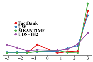
Figure 2: Relative frequency of factuality ratings in training and development sets.

Pre-processing

To compare model results on UDS-IH2 to those found in the unified datasets of Stanovsky et al. (2017), we map the happened and confidence ratings to a single factuality value in [-3,3] by first taking the mean confidence rating for each predicate and mapping factuality to $\frac{3}{4}$confidence if happened and -$\frac{3}{4}$confidence otherwise.

Response distribution

Figure 2 plots the distribution of factuality ratings in the train and dev splits for UDS-IH2, alongside those of FactBank, UW, and MEANTIME. One striking feature of these distributions is that UDS-IH2 displays a much more entropic distribution than the other datasets. This may be due to the fact that, unlike the newswire-heavy corpora that the other datasets annotate, EUD1.2 contains text from genres – weblogs, newsgroups, email, reviews, and question-answers – that tend to involve less reporting of raw facts. One consequence of this more entropic distribution is that, unlike the datasets discussed above, it is much harder for systems that always guess 3 – i.e. factual with high confidence/likelihood – to perform well.

4 Models

We consider two neural models of factuality: a stacked bidirectional linear chain LSTM (§4.1) and a stacked bidirectional child-sum dependency tree LSTM (§4.2). To predict the factuality $v_{t}$ for the event referred to by a word $w_{t}$, we use the hidden state at $t$ from the final layer of the stack as the input to a two-layer regression model (§4.3).

4.1 Stacked bidirectional linear LSTM

We use a standard stacked bidirectional linear chain LSTM (stacked L-biLSTM), which extends the unidirectional linear chain LSTM (Hochreiter and Schmidhuber, 1997) by adding the notion of a layer $l\in\{1,\ldots,L\}$ and a direction $d\in\{\rightarrow,\leftarrow\}$ (Graves et al., 2013; Sutskever et al., 2014; Zaremba and Sutskever, 2014).

$\displaystyle\begin{aligned} \mathbf{f}^{(l,d)}_{t}&=\sigma\left(\mathbf{W}^{(l,d)}_{\mathrm{f}}\left[\mathbf{h}^{(l,d)}_{\mathbf{prev}_{d}(t)};\mathbf{x}^{(l,d)}_{t}\right]+\mathbf{b}^{(l,d)}_{\mathrm{f}}\right)\\ \mathbf{i}^{(l,d)}_{t}&=\sigma\left(\mathbf{W}^{(l,d)}_{\mathrm{i}}\left[\mathbf{h}^{(l,d)}_{\mathbf{prev}_{d}(t)};\mathbf{x}^{(l,d)}_{t}\right]+\mathbf{b}^{(l,d)}_{\mathrm{i}}\right)\\ \mathbf{o}^{(l,d)}_{t}&=\sigma\left(\mathbf{W}^{(l,d)}_{\mathrm{o}}\left[\mathbf{h}^{(l,d)}_{\mathbf{prev}_{d}(t)};\mathbf{x}^{(l,d)}_{t}\right]+\mathbf{b}^{(l,d)}_{\mathrm{o}}\right)\\ \hat{\mathbf{c}}^{(l,d)}_{t}&=g\left(\mathbf{W}^{(l,d)}_{\mathrm{c}}\left[\mathbf{h}^{(l,d)}_{\mathbf{prev}_{d}(t)};\mathbf{x}^{(l,d)}_{t}\right]+\mathbf{b}^{(l,d)}_{\mathrm{c}}\right)\\ \mathbf{c}^{(l,d)}_{t}&=\mathbf{i}^{(l,d)}_{t}\circ\hat{\mathbf{c}}^{(l,d)}_{t}+\mathbf{f}^{(l,d)}_{t}\circ\mathbf{c}^{(l,d)}_{\mathbf{prev}_{d}(t)}\\ \mathbf{h}^{(l,d)}_{t}&=\mathbf{o}^{(l,d)}_{t}\circ g\left(\mathbf{c}^{(l,d)}_{t}\right)\\ \end{aligned}$

where $\circ$ is the Hadamard product; $\mathbf{prev}_{\rightarrow}(t)=t-1$ and $\mathbf{prev}_{\leftarrow}(t)=t+1$, and $\mathbf{x}^{(l,d)}_{t}=\mathbf{x}_{t}$ if $l=1$; and $\mathbf{x}^{(l,d)}_{t}=[\mathbf{h}^{(l-1,\rightarrow)}_{t};\mathbf{h}^{(l-1,\leftarrow)}_{t}]$ otherwise. We set $g$ to the pointwise nonlinearity tanh.

4.2 Stacked bidirectional tree LSTM

We use a stacked bidirectional extension to the child-sum dependency tree LSTM (T-LSTM; Tai et al., 2015), which is itself an extension of a standard unidirectional linear chain LSTM (L-LSTM). One way to view the difference between the L-LSTM and the T-LSTM is that the T-LSTM redefines $\mathbf{prev}_{\rightarrow}(t)$ to return the set of indices that correspond to the children of $w_{t}$ in some dependency tree. Because the cardinality of these sets varies with $t$, it is necessary to specify how multiple children are combined. The basic idea, which we make explicit in the equations for our extension, is to define $\mathbf{f}_{tk}$ for each child index $k\in\mathbf{prev}_{\rightarrow}(t)$ in a way analogous to the equations in §4.1 – i.e. as though each child were the only child – and then sum across $k$ within the equations for $\mathbf{i}_{t}$, $\mathbf{o}_{t}$, $\hat{\mathbf{c}}_{t}$, $\mathbf{c}_{t}$, and $\mathbf{h}_{t}$.

Our stacked bidirectional extension (stacked T-biLSTM) is a minimal extension to the T-LSTM in the sense that we merely define the downward computation in terms of a $\mathbf{prev}_{\leftarrow}(t)$ that returns the set of indices that correspond to the parents of $w_{t}$ in some dependency tree (cf. Miwa and Bansal 2016, who propose a similar, but less minimal, model for relation extraction). The same method for combining children in the upward computation can then be used for combining parents in the downward computation. This yields a minimal change to the stacked L-biLSTM equations.

$\displaystyle\begin{aligned} \mathbf{f}^{(l,d)}_{tk}&=\sigma\left(\mathbf{W}^{(l,d)}_{\mathrm{f}}\left[\mathbf{h}^{(l,d)}_{k};\mathbf{x}^{(l,d)}_{t}\right]+\mathbf{b}^{(l,d)}_{\mathrm{f}}\right)\\ \hat{\mathbf{h}}^{(l,d)}_{t}&=\sum_{k\in\mathbf{prev}_{d}(t)}\mathbf{h}^{(l,d)}_{k}\\ \mathbf{i}^{(l,d)}_{t}&=\sigma\left(\mathbf{W}^{(l,d)}_{\mathrm{i}}\left[\hat{\mathbf{h}}^{(l,d)}_{t};\mathbf{x}^{(l,d)}_{t}\right]+\mathbf{b}^{(l,d)}_{\mathrm{i}}\right)\\ \mathbf{o}^{(l,d)}_{t}&=\sigma\left(\mathbf{W}^{(l,d)}_{\mathrm{o}}\left[\hat{\mathbf{h}}^{(l,d)}_{t};\mathbf{x}^{(l,d)}_{t}\right]+\mathbf{b}^{(l,d)}_{\mathrm{o}}\right)\\ \hat{\mathbf{c}}^{(l,d)}_{t}&=g\left(\mathbf{W}^{(l,d)}_{\mathrm{c}}\left[\hat{\mathbf{h}}^{(l,d)}_{t};\mathbf{x}^{(l,d)}_{t}\right]+\mathbf{b}^{(l,d)}_{\mathrm{c}}\right)\\ \mathbf{c}^{(l,d)}_{t}&=\mathbf{i}^{(l,d)}_{t}\circ\hat{\mathbf{c}}^{(l,d)}_{t}+\sum_{k\in\mathbf{prev}_{d}(t)}\mathbf{f}^{(l,d)}_{tk}\circ\mathbf{c}^{(l,d)}_{k}\\ \mathbf{h}^{(l,d)}_{t}&=\mathbf{o}^{(l,d)}_{t}\circ g\left(\mathbf{c}^{(l,d)}_{t}\right)\\ \end{aligned}$

We use a ReLU pointwise nonlinearity for $g$. These minimal changes allow us to represent the inside and the outside contexts of word $t$ (at layer $l$) as single vectors: $\hat{\mathbf{h}}^{(l,\rightarrow)}_{t}$ and $\hat{\mathbf{h}}^{(l,\leftarrow)}_{t}$.

An important thing to note here is that – in contrast to other dependency tree-structured T-LSTMs (Socher et al., 2014; Iyyer et al., 2014) – this T-biLSTM definition does not use the dependency labels in any way. Such labels could be straightforwardly incorporated to determine which parameters are used in a particular cell, but for current purposes, we retain the simpler structure (i) to more directly compare the L- and T-biLSTMs and (ii) because a model that uses dependency labels substantially increases the number of trainable parameters, relative to the size of our datasets.

4.3 Regression model

To predict the factuality $v_{t}$ for the event referred to by a word $w_{t}$, we use the hidden states from the final layer of the stacked L- or T-biLSTM as the input to a two-layer regression model.

$\displaystyle\begin{aligned} \mathbf{h}^{(L)}_{t}&=[\mathbf{h}^{(L,\rightarrow)}_{t};\mathbf{h}^{(L,\leftarrow)}_{t}]\\ \hat{v_{t}}&=\mathbf{V}_{2}\;g\left(\mathbf{V}_{1}\mathbf{h}^{(L)}_{t}+\mathbf{b}_{1}\right)+\mathbf{b}_{2}\end{aligned}$

where $\hat{v_{t}}$ is passed to a loss function $\mathbb{L}(\hat{v_{t}},v_{t})$: in this case, smooth L1 – i.e. Huber loss with $\delta=1$. This loss function is effectively a smooth variant of the hinge loss used by Lee et al. (2015) and Stanovsky et al. (2017).

We also consider a simple ensemble method, wherein the hidden states from the final layers of both the stacked L-biLSTM and the stacked T-biLSTM are concatenated and passed through the same two-layer regression model. We refer to this as the H(ybrid)-biLSTM.

5 Experiments

Implementation

We implement both the L-biLSTM and T-biLSTM models using pytorch 0.2.0. The L-biLSTM model uses the stock implementation of the stacked bidirectional linear chain LSTM found in pytorch, and the T-biLSTM model uses a custom implementation, which we make available at decomp.net.

Word embeddings

We use the 300-dimensional GloVe 42B uncased word embeddings (Pennington et al., 2014) with an UNK embedding whose dimensions are sampled iid from a Uniform[-1,1]. We do not tune these embeddings during training.

Hidden state sizes

We set the dimension of the hidden states $\mathbf{h}_{t}^{(l,d)}$ and cell states $\mathbf{c}_{t}^{(l,d)}$ to 300 for all layers of the stacked L- and stacked T-biLSTMs – the same size as the input word embeddings. This means that the input to the regression model is 600-dimensional, for the stacked L- and T-biLSTMs, and 1200-dimensional, for the stacked H-biLSTM. For the hidden layer of the regression component, we set the dimension to half the size of the input hidden state: 300, for the stacked L- and T-biLSTMs, and 600, for the stacked H-biLSTM.

Bidirectional layers

We consider stacked L-, T-, and H-biLSTMs with either one or two layers. In preliminary experiments, we found that networks with three layers badly overfit the training data.

Verb	Signature	Type	Example
know	$+|+$	fact.	Jo knew that Bo ate.
manage	$+|-$	impl.	Jo managed to go.
neglect	$-|+$	impl.	Jo neglected to call Bo.
hesitate	$\circ|+$	impl.	Jo didn’t hesitate to go.
attempt	$\circ|-$	impl.	Jo didn’t attempt to go.

Table 2: Implication signature features from Nairn et al. (2006). As an example, a signature of $-|+$ indicates negative implication under positive polarity (left side) and positive implication under negative polarity (right side); $\circ$ indicates neither positive nor negative implication.

Dependency parses

For the T- and H-biLSTMs, we use the gold dependency parses provided in EUD1.2 when training and testing on UDS-IH2. On FactBank, MEANTIME, and UW, we follow Stanovsky et al. (2017) in using the automatic dependency parses generated by the parser in spaCy (Honnibal and Johnson, 2015).

Lexical features

Recent work on neural models in the closely related domain of genericity/habituality prediction suggests that inclusion of hand-annotated lexical features can improve classification performance (Becker et al., 2017). To assess whether similar performance gains can be obtained here, we experiment with lexical features for simple factive and implicative verbs Kiparsky and Kiparsky (1970); Karttunen (1971a). When in use, these features are concatenated to the network’s input word embeddings so that, in principle, they may interact with one another and inform other hidden states in the biLSTM, akin to how verbal implicatives and factives are observed to influence the factuality of their complements. The hidden state size is increased to match the input embedding size. We consider two types:

Signature features We compute binary features based on a curated list of 92 simple implicative and 95 factive verbs including their their type-level “implication signatures,” as compiled by Nairn et al. (2006). These signatures characterize the implicative or factive behavior of a verb with respect to its complement clause, how this behavior changes (or does not change) under negation, and how it composes with other such verbs under nested recursion. We create one indicator feature for each signature type.

Mined features Using a simplified set of pattern matching rules over Common Crawl data Buck et al. (2014), we follow the insights of Pavlick and Callison-Burch (2016) – henceforth, PC – and use corpus mining to automatically score verbs for implicativeness. The insight of PC lies in Karttunen’s (1971a) observation that “the main sentence containing an implicative predicate and the complement sentence necessarily agree in tense.”

Accordingly, PC devise a tense agreement score – effectively, the ratio of times an embedding predicate’s tense matches the tense of the predicate it embeds – to predict implicativeness in English verbs. Their scoring method involves the use of fine-grained POS tags, the Stanford Temporal Tagger (Chang and Manning, 2012), and a number of heuristic rules, which resulted in a confirmation that tense agreement statistics are predictive of implicativeness, illustrated in part by observing a near perfect separation of a list of implicative and non-implicative verbs from Karttunen (1971a).

dare to	1.00	intend to	0.83
bother to	1.00	want to	0.77
happen to	0.99	decide to	0.75
forget to	0.99	promise to	0.75
manage to	0.97	agree to	0.35
try to	0.96	plan to	0.20
get to	0.90	hope to	0.05
venture to	0.85

Table 3: Implicative (bold) and non-implicative (not bold) verbs from Karttunen (1971a) are nearly separable by our tense agreement scores, replicating the results of PC.

	FactBank		UW		Meantime		UDS-IH2
	MAE	r	MAE	r	MAE	r	MAE	r
All-3.0	0.8	NAN	0.78	NAN	0.31	NAN	2.255	NAN
Lee et al. 2015	-	-	0.511	0.708	-	-	-	-
Stanovsky et al. 2017	0.59	0.71	0.42†	0.66	0.34	0.47	-	-
L-biLSTM(2)-S	0.427	0.826	0.508	0.719	0.427	0.335	0.960†	0.768
T-biLSTM(2)-S	0.577	0.752	0.600	0.645	0.428	0.094	1.101	0.704
L-biLSTM(2)-G	0.412	0.812	0.523	0.703	0.409	0.462	-	-
T-biLSTM(2)-G	0.455	0.809	0.567	0.688	0.396	0.368	-	-
L-biLSTM(2)-S+lexfeats	0.429	0.796	0.495	0.730	0.427	0.322	1.000	0.755
T-biLSTM(2)-S+lexfeats	0.542	0.744	0.567	0.676	0.375	0.242	1.087	0.719
L-biLSTM(2)-MultiSimp	0.353	0.843	0.503	0.725	0.345	0.540	-	-
T-biLSTM(2)-MultiSimp	0.482	0.803	0.599	0.645	0.545	0.237	-	-
L-biLSTM(2)-MultiBal	0.391	0.821	0.496	0.724	0.278	0.613†	-	-
T-biLSTM(2)-MultiBal	0.517	0.788	0.573	0.659	0.400	0.405	-	-
L-biLSTM(1)-MultiFoc	0.343	0.823	0.516	0.698	0.229†	0.599	-	-
L-biLSTM(2)-MultiFoc	0.314	0.846	0.502	0.710	0.305	0.377	-	-
T-biLSTM(2)-MultiFoc	1.100	0.234	0.615	0.616	0.395	0.300	-	-
L-biLSTM(2)-MultiSimp w/UDS-IH2	0.377	0.828	0.508	0.722	0.367	0.469	0.965	0.771†
T-biLSTM(2)-MultiSimp w/UDS-IH2	0.595	0.716	0.598	0.609	0.467	0.345	1.072	0.723
H-biLSTM(2)-S	0.488	0.775	0.526	0.714	0.442	0.255	0.967	0.768
H-biLSTM(1)-MultiSimp	0.313†	0.857†	0.528	0.704	0.314	0.545	-	-
H-biLSTM(2)-MultiSimp	0.431	0.808	0.514	0.723	0.401	0.461	-	-
H-biLSTM(2)-MultiBal	0.386	0.825	0.502	0.713	0.352	0.564	-	-
H-biLSTM(2)-MultiSimp w/UDS-IH2	0.393	0.820	0.481	0.749†	0.374	0.495	0.969	0.760

Table 4: All 2-layer systems, and 1-layer systems if best in column. State-of-the-art results in bold; ^† indicates best in column (corresponding row shaded in purple). Key: L=linear, T=tree, H=hybrid, (1,2)=# layers, S=single-task specific, G=single-task general, +lexfeats=with all lexical features, MultiSimp=multi-task simple, MultiBal=multi-task balanced, MultiFoc=multi-task focused, w/UDS-IH2=trained on all data including UDS-IH2. All-3.0 is a constant baseline, always predicting 3.0.

We replicate this finding by employing a simplified pattern matching method over 3B sentences of raw Common Crawl text. We efficiently search for instances of any pattern of the form: I $VERB to * $TIME, where $VERB and $TIME are pre-instantiated variables so their corresponding tenses are known, and ‘*’ matches any one to three whitespace-separated tokens at runtime (not pre-instantiated). Our results in Table 3 are a close replication of PC’s findings. Prior work such as by PC is motivated in part by the potential for corpus-linguistic findings to be used as fodder in downstream predictive tasks: we include these agreement scores as potential input features to our networks to test whether contemporary models do in fact benefit from this information.

Training

For all experiments, we use stochastic gradient descent to train the LSTM parameters and regression parameters end-to-end with the Adam optimizer (Kingma and Ba, 2015), using the default learning rate in pytorch (1e-3). We consider five training regimes:

1. single-task specific (-S) Train a separate instance of the network for each dataset, training only on that dataset.

2. single-task general (-G) Train one instance of the network on the simple concatenation of all unified factuality datasets, {FactBank, UW, MEANTIME}.

3. multi-task simple (-MultiSimp) Same as single-task general, except the network maintains a distinct set of regression parameters for each dataset; all other parameters (LSTM) remain tied. “w/UDS-IH2” is specified if UDS-IH2 is included in training.

4. multi-task balanced (-MultiBal) Same as multi-task simple but upsampling examples from the smaller datasets to ensure that examples from those datasets are seen at the same rate.

5. multi-task focused (-MultiFoc) Same as multi-task simple but upsampling examples from a particular target dataset to ensure that examples from that dataset are seen 50% of the time and examples from the other datasets are seen 50% (evenly distributed across the other datasets).

Calibration

Post-training, network predictions are monotonically re-adjusted to a specific dataset using isotonic regression (fit on train split only).

		Mean	Linear	Tree
Modal	Negated	Label	MAE	MAE	#
none	no	1.00	0.93	1.03	2244
none	yes	-0.19	1.40	1.69	98
may	no	-0.38	1.00	0.99	14
would	no	-0.61	0.85	0.99	39
ca(n’t)	yes	-0.72	1.28	1.55	11
can	yes	-0.75	0.99	0.86	6
(wi)’ll	no	-0.94	1.47	1.14	8
could	no	-1.03	0.97	1.32	20
can	no	-1.25	1.02	1.21	73
might	no	-1.25	0.66	1.06	6
would	yes	-1.27	0.40	0.86	5
should	no	-1.31	1.20	1.01	22
will	no	-1.88	0.75	0.86	75

Table 5: Mean gold labels, counts, and MAE for L-biLSTM(2)-S and T-biLSTM(2)-S model predictions on UDS-IH2-dev, grouped by modals and negation.

Evaluation

Following Lee et al. (2015) and Stanovsky et al. (2017), we report two evaluation measures: mean absolute error (MAE) and Pearson correlation (r). We would like to note, however, that we believe correlation to be a better indicator of performance for two reasons: (i) for datasets with a high degree of label imbalance (Figure 2), a baseline that always guesses the mean or mode label can be difficult to beat in terms of MAE but not correlation, and (ii) MAE is harder to meaningfully compare across datasets with different label mean and variance.

Development

Under all regimes, we train the model for 20 epochs – by which time all models appear to converge. We save the parameter values after the completion of each epoch and then score each set of saved parameter values on the development set for each dataset. The set of parameter values that performed best on dev in terms of Pearson correlation for a particular dataset were then used to score the test set for that dataset.

6 Results

Table 4 reports the results for all of the 2-layer L-, T-, and H-biLSTMs. The best-performing system for each dataset and metric are highlighted in purple, and when the best-performing system for a particular dataset was a 1-layer model, that system is included in Table 4.

New state of the art

For each dataset and metric, with the exception of MAE on UW, we achieve state of the art results with multiple systems. The highest-performing system for each is reported in Table 4. Our results on UDS-IH2 are the first reported numbers for this new factuality resource.

	Mean
Relation	Label	L-biLSTM	T-biLSTM	#
root	1.07	1.03	0.96	949
conj	0.37	0.44	0.46	316
advcl	0.46	0.53	0.45	303
xcomp	-0.42	-0.57	-0.49	234
acl:relcl	1.28	1.40	1.31	193
ccomp	0.11	0.31	0.34	191
acl	0.77	0.59	0.58	159
parataxis	0.44	0.63	0.79	127
amod	1.92	1.88	1.81	76
csubj	0.36	0.38	0.27	37

Table 6: Mean predictions for linear (L-biLSTM-S(2)) and tree models (T-biLSTM-S(2)) on UDS-IH2-dev, grouped by governing dependency relation. Only the 10 most frequent governing dependency relations in UDS-IH2-dev are shown.

Linear v. tree topology

On its own, the biLSTM with linear topology (L-biLSTM) performs consistently better than the biLSTM with tree topology (T-biLSTM). However, the hybrid topology (H-biLSTM), consisting of both a L- and T-biLSTM is the top-performing system on UW for correlation (Table 4). This suggests that the T-biLSTM may be contributing something complementary to the L-biLSTM.

Evidence of this complementarity can be seen in Table 6, which contains a breakdown of system performance by governing dependency relation, for both linear and tree models, on UDS-IH2-dev. In most cases, the L-biLSTM’s mean prediction is closer to the true mean. This appears to arise in part because the T-biLSTM is less confident in its predictions – i.e. its mean prediction tends to be closer to 0. This results in the L-biLSTM being too confident in certain cases – e.g. in the case of the xcomp governing relation, where the T-biLSTM mean prediction is closer to the true mean.

Lexical features have minimal impact

Adding all lexical features (both signature and mined) yields mixed results. We see slight improvements on UW, while performance on the other datasets mostly declines (compare with single-task specific). Factuality prediction is precisely the kind of NLP task one would expect these types of features to assist with, so it is notable that, in our experiments, they do not.

Multi-task helps

Though our methods achieve state of the art in the single-task setting, the best performing systems are mostly multi-task (Table 4 and Supplementary Materials). This is an ideal setting for multi-task training: each dataset is relatively small, and their labels capture closely-related (if not identical) linguistic phenomena. UDS-IH2, the largest by a factor of two, reaps the smallest gains from multi-task.

7 Analysis

As discussed in §2, many discrete linguistic phenomena interact with event factuality. Here we provide a brief analysis of some of those interactions, both as they manifest in the UDS-IH2 dataset, as well as in the behavior of our models. This analysis employs the gold dependency parses present in EUD1.2.

Table 5 illustrates the influence of modals and negation on the factuality of the events they have direct scope over. The context with the highest factuality on average is no direct modal and no negation (first row); all other modal contexts have varying degrees of negative mean factuality scores, with will as the most negative. This is likely a result of UDS-IH2 annotation instructions to mark future events as not having happened.

Attribute	#
Grammatical error present, incl. run-ons	16
Is an auxiliary or light verb	14
Annotation is incorrect	13
Future event	12
Is a question	5
Is an imperative	3
Is not an event or state	2
One or more of the above	43

Table 7: Notable attributes of 50 instances from UDS-IH2-dev with highest absolute prediction error (using H-biLSTM(2)-MultiSim w/UDS-IH2).

Table 7 shows results from a manual error analysis on 50 events from UDS-IH2-dev with highest absolute prediction error (using H-biLSTM(2)-MultiSim w/UDS-IH2). Grammatical errors (such as run-on sentences) in the underlying text of UDS-IH2 appear to pose a particular challenge for these models; informal language and grammatical errors in UDS-IH2 is a substantial distinction from the other factuality datasets used here.

manage to	2.78	agree to	-1.00
happen to	2.34	forget to	-1.18
dare to	1.50	want to	-1.48
bother to	1.50	intend to	-2.02
decide to	0.10	promise to	-2.34
get to	-0.23	plan to	-2.42
try to	-0.24	hope to	-2.49

Table 8: UDS-IH2-train: Infinitival-taking verbs sorted by the mean annotation scores of their complements (xcomp), with direct negation filtered out. Implicatives are in bold.

In §6 we observe that the linguistically-motivated lexical features that we test (+lexfeats) do not have a big impact on overall performance. Tables 8 and 9 help nuance this observation.

Table 8 shows that we can achieve similar separation between implicatives and non-implicatives as the feature mining strategy presented in §5. That is, those features may be redundant with information already learnable from factuality datasets (UDS-IH2). Despite the underperformance of these features overall, Table 9 shows that they may still improve performance in the subset of instances where they appear.

Verb	L-biLSTM(2)-S	+lexfeats	#
decide to	3.28	2.66	2
forget to	0.67	0.48	2
get to	1.55	1.43	9
hope to	1.35	1.23	5
intend to	1.18	0.61	1
promise to	0.40	0.49	1
try to	1.14	1.42	12
want to	1.22	1.17	24

Table 9: MAE of L-biLSTM(2)-S and L-biLSTM(2)-S+lexfeats, for predictions on events in UDS-IH2-dev that are xcomp-governed by an infinitival-taking verb.

8 Conclusion

We have proposed two neural models of event factuality prediction – a bidirectional linear-chain LSTM (L-biLSTM) and a bidirectional child-sum dependency tree LSTM (T-biLSTM) – which yield substantial performance gains over previous models based on deterministic rules and hand-engineered features. We found that both models yield such gains, though the L-biLSTM generally outperforms the T-biLSTM; for some datasets, a simple ensemble of the two (H-biLSTM) improves over either alone.

We have also extended the UDS-IH1 dataset, yielding the largest publicly-available factuality dataset to date: UDS-IH2. In experiments, we see substantial gains from multi-task training over the three factuality datasets unified by Stanovsky et al. (2017), as well as UDS-IH2. Future work will further probe the behavior of these models, or extend them to learn other aspects of event semantics.

Appendix A Appendix

A.1 Dataset filtering

We filter our dataset to remove annotators with very low agreement in two ways: (i) based on the their agreement with other annotators on the happened question; and (ii) based on the their agreement with other annotators on the confidence question.

For the happened question, we computed, for each pair of annotators and each item that both of those annotators annotated, whether the two responses were equal. We then fit a random effects logistic regression to response equality with random intercepts for annotator. The Best Linear Unbiased Predictors (BLUPs) for each annotator were then extracted and $z$-scored. Annotators were removed if their $z$-scored BLUP was less than -2.

For the confidence question, we first ridit-scored the ratings by annotator; and for each pair of annotators and each item that both of those annotators annotated, we computed the difference between the two ridit-scored confidences. We then fit a random effects linear regression to the resulting difference after logit-transformation with random intercepts for annotator. The same BLUP-based exclusion procedure was then used.

This filtering results in the exclusion of one annotator, who is excluded for low agreement on happened. 4,179 annotations are removed in the filtering, but because we remove only a single annotator, there remains at least one annotation for every predicate.

A.2 Mining Implicatives

All options for instantiating the $TIME pattern variable, described in §5, are listed here.

• Past Tense Phrases: earlier today, yesterday, last week, last month, last year

• Future Tense Phrases: later today, tomorrow, next week, next month, next year

A.3 Full Results

Table 10 presents the full set of results, including all 1-layer and 2-layer models, and performance on development splits.

	FactBank				UW				Meantime				UD
	dev		test		dev		test		dev		test		dev		test
	MAE	r	MAE	r	MAE	r	MAE	r	MAE	r	MAE	r	MAE	r	MAE	r
All-3.0	-	-	0.8	0	-	-	0.78	0	-	-	0.31	0	-	-	2.255	0
Lee et al. 2015	-	-	-	-	0.462	0.749	0.511	0.708	-	-	-	-	-	-	-	-
Stanovsky et al. 2017	-	-	0.59	0.71	-	-	0.42	0.66	-	-	0.31	0.47	-	-	-	-
L-biLSTM(1)-S	0.411	0.78	0.399	0.816	0.435	0.797	0.508	0.718	0.239	0.631	0.337	0.359	0.978	0.768	0.986	0.765
L-biLSTM(2)-S	0.482	0.772	0.427	0.826	0.426	0.799	0.508	0.719	0.357	0.601	0.427	0.335	0.95	0.771	0.96	0.768
T-biLSTM(1)-S	0.564	0.711	0.48	0.748	0.491	0.734	0.574	0.652	0.297	0.564	0.36	0.155	1.043	0.739	1.053	0.725
T-biLSTM(2)-S	0.595	0.71	0.577	0.752	0.497	0.735	0.6	0.645	0.351	0.371	0.428	0.094	1.06	0.719	1.101	0.704
L-biLSTM(1)-G	0.432	0.798	0.383	0.819	0.426	0.807	0.517	0.717	0.252	0.625	0.343	0.505	-	-	-	-
L-biLSTM(2)-G	0.439	0.799	0.412	0.812	0.42	0.809	0.523	0.703	0.291	0.604	0.409	0.462	-	-	-	-
T-biLSTM(1)-G	0.468	0.758	0.405	0.82	0.472	0.76	0.571	0.662	0.336	0.509	0.408	0.384	-	-	-	-
T-biLSTM(2)-G	0.498	0.764	0.455	0.809	0.481	0.757	0.567	0.688	0.298	0.527	0.396	0.368	-	-	-	-
L-biLSTM(1)-S+lexfeats:sign	0.423	0.78	0.396	0.805	-	-	-	-	-	-	-	-	-	-	-	-
L-biLSTM(2)-S+lexfeats:sign	0.459	0.768	0.423	0.82	-	-	-	-	-	-	-	-	-	-	-	-
T-biLSTM(1)-S+lexfeats:sign	0.54	0.718	0.51	0.762	-	-	-	-	-	-	-	-	-	-	-	-
T-biLSTM(2)-S+lexfeats:sign	0.552	0.731	0.558	0.748	-	-	-	-	-	-	-	-	-	-	-	-
L-biLSTM(1)-S+lexfeats:mine	0.468	0.781	0.453	0.801	-	-	-	-	-	-	-	-	-	-	-	-
L-biLSTM(2)-S+lexfeats:mine	0.416	0.768	0.373	0.808	-	-	-	-	-	-	-	-	-	-	-	-
T-biLSTM(1)-S+lexfeats:mine	0.546	0.725	0.525	0.751	-	-	-	-	-	-	-	-	-	-	-	-
T-biLSTM(2)-S+lexfeats:mine	0.567	0.727	0.573	0.72	-	-	-	-	-	-	-	-	-	-	-	-
L-biLSTM(1)-S+lexfeats:both	0.443	0.781	0.413	0.805	0.428	0.803	0.507	0.722	0.319	0.481	0.373	0.369	1.002	0.762	1.002	0.766
L-biLSTM(2)-S+lexfeats:both	0.485	0.764	0.429	0.796	0.433	0.792	0.495	0.73	0.356	0.662	0.427	0.322	0.977	0.767	1	0.755
T-biLSTM(1)-S+lexfeats:both	0.503	0.728	0.449	0.793	0.485	0.743	0.589	0.643	0.282	0.493	0.348	0.191	1.04	0.738	1.073	0.718
T-biLSTM(2)-S+lexfeats:both	0.565	0.724	0.542	0.744	0.481	0.747	0.567	0.676	0.352	0.404	0.375	0.242	1.049	0.738	1.087	0.719
L-biLSTM(1)-MultiSimp	0.408	0.804	0.365	0.834	0.414	0.825	0.506	0.736	0.241	0.506	0.286	0.453	-	-	-	-
L-biLSTM(2)-MultiSimp	0.393	0.811	0.353	0.843	0.417	0.817	0.503	0.725	0.314	0.56	0.345	0.54	-	-	-	-
T-biLSTM(1)-MultiSimp	0.464	0.756	0.408	0.807	0.472	0.754	0.555	0.67	0.248	0.546	0.318	0.357	-	-	-	-
T-biLSTM(2)-MultiSimp	0.517	0.753	0.482	0.803	0.493	0.754	0.599	0.645	0.474	0.52	0.545	0.237	-	-	-	-
L-biLSTM(1)-MultiBal	0.387	0.805	0.332	0.841	0.412	0.822	0.52	0.722	0.232	0.57	0.256	0.544	-	-	-	-
L-biLSTM(2)-MultiBal	0.441	0.8	0.391	0.821	0.414	0.815	0.496	0.724	0.251	0.624	0.278	0.613	-	-	-	-
T-biLSTM(1)-MultiBal	0.475	0.746	0.405	0.817	0.472	0.752	0.578	0.629	0.237	0.56	0.344	0.266	-	-	-	-
T-biLSTM(2)-MultiBal	0.56	0.73	0.517	0.788	0.499	0.734	0.573	0.659	0.252	0.567	0.4	0.405	-	-	-	-
L-biLSTM(1)-MultiFoc	0.378	0.79	0.343	0.823	0.414	0.813	0.516	0.698	0.256	0.48	0.229	0.599	-	-	-	-
L-biLSTM(2)-MultiFoc	0.379	0.808	0.314	0.846	0.409	0.81	0.502	0.71	0.227	0.524	0.305	0.377	-	-	-	-
T-biLSTM(1)-MultiFoc	0.469	0.748	0.401	0.81	0.474	0.754	0.579	0.654	0.29	0.533	0.354	0.293	-	-	-	-
T-biLSTM(2)-MultiFoc	1.091	0.231	1.1	0.234	0.508	0.731	0.615	0.616	0.293	0.456	0.395	0.3	-	-	-	-
L-biLSTM(1)-MultiSimp w/UDS-IH2	0.417	0.802	0.381	0.813	0.421	0.802	0.486	0.741	0.385	0.51	0.353	0.565	0.972	0.771	0.977	0.765
L-biLSTM(2)-MultiSimp w/UDS-IH2	0.439	0.794	0.377	0.828	0.418	0.803	0.508	0.722	0.305	0.541	0.367	0.469	0.959	0.774	0.965	0.771
T-biLSTM(1)-MultiSimp w/UDS-IH2	0.535	0.732	0.498	0.778	0.492	0.746	0.611	0.61	0.377	0.44	0.413	0.395	1.061	0.735	1.069	0.728
T-biLSTM(2)-MultiSimp w/UDS-IH2	0.597	0.717	0.595	0.716	0.526	0.706	0.598	0.609	0.427	0.471	0.467	0.345	1.048	0.736	1.072	0.723
H-biLSTM(1)-S	0.42	0.789	0.378	0.831	0.427	0.804	0.518	0.704	0.349	0.437	0.405	0.085	0.989	0.767	0.992	0.765
H-biLSTM(2)-S	0.505	0.739	0.488	0.775	0.467	0.765	0.526	0.714	0.352	0.595	0.442	0.255	0.948	0.775	0.967	0.768
H-biLSTM(1)-MultiSimp	0.395	0.802	0.313	0.857	0.417	0.821	0.528	0.704	0.267	0.601	0.314	0.545	-	-	-	-
H-biLSTM(2)-MultiSimp	0.472	0.77	0.431	0.808	0.431	0.792	0.514	0.723	0.359	0.547	0.401	0.461	-	-	-	-
H-biLSTM(1)-MultiBal	0.398	0.803	0.334	0.853	0.402	0.829	0.497	0.733	0.229	0.59	0.264	0.432	-	-	-	-
H-biLSTM(2)-MultiBal	0.42	0.797	0.386	0.825	0.418	0.811	0.502	0.713	0.302	0.571	0.352	0.564	-	-	-	-
H-biLSTM(1)-MultiSimp w/UDS-IH2	0.431	0.785	0.365	0.833	0.431	0.8	0.513	0.733	0.277	0.569	0.341	0.286	0.982	0.765	0.98	0.761
H-biLSTM(2)-MultiSimp w/UDS-IH2	0.44	0.79	0.393	0.82	0.422	0.815	0.481	0.749	0.306	0.556	0.374	0.495	0.97	0.764	0.969	0.76

Table 10: Full table of results, including all 1-layer and 2-layer models.

References

- Becker et al. (2017) Maria Becker, Michael Staniek, Vivi Nastase, Alexis Palmer, and Anette Frank. 2017. Classifying Semantic Clause Types: Modeling Context and Genre Characteristics with Recurrent Neural Networks and Attention. In Proceedings of the 6th Joint Conference on Lexical and Computational Semantics (*SEM 2017). pages 230–240.
- Bowman et al. (2016) Samuel R Bowman, Jon Gauthier, Abhinav Rastogi, Raghav Gupta, Christopher D Manning, and Christopher Potts. 2016. A fast unified model for parsing and sentence understanding. In Proceedings of the 54th Annual Meeting of the Association for Computational Linguistics. Association for Computational Linguistics, Berlin, Germany, pages 1466–1477.
- Bowman et al. (2015) Samuel R. Bowman, Christopher Potts, and Christopher D. Manning. 2015. Learning distributed word representations for natural logic reasoning. In Proceedings of the AAAI Spring Symposium on Knowledge Representation and Reasoning.
- Buck et al. (2014) Christian Buck, Kenneth Heafield, and Bas van Ooyen. 2014. N-gram Counts and Language Models from the Common Crawl. In Proceedings of the Ninth International Conference on Language Resources and Evaluation (LREC-2014). European Language Resources Association (ELRA), Reykjavik, Iceland.
- Chang and Manning (2012) Angel X. Chang and Christopher Manning. 2012. Sutime: A library for recognizing and normalizing time expressions. In Nicoletta Calzolari (Conference Chair), Khalid Choukri, Thierry Declerck, Mehmet Uğur Doğan, Bente Maegaard, Joseph Mariani, Asuncion Moreno, Jan Odijk, and Stelios Piperidis, editors, Proceedings of the Eight International Conference on Language Resources and Evaluation (LREC’12). European Language Resources Association (ELRA), Istanbul, Turkey.
- de Marneffe et al. (2012) Marie-Catherine de Marneffe, Christopher D. Manning, and Christopher Potts. 2012. Did it happen? The pragmatic complexity of veridicality assessment. Computational Linguistics 38(2):301–333.
- Diab et al. (2009) Mona T Diab, Lori Levin, Teruko Mitamura, Owen Rambow, Vinodkumar Prabhakaran, and Weiwei Guo. 2009. Committed belief annotation and tagging. In Proceedings of the Third Linguistic Annotation Workshop. Association for Computational Linguistics, pages 68–73.
- Egré (2008) Paul Egré. 2008. Question-embedding and factivity. Grazer Philosophische Studien 77(1):85–125.
- Graves et al. (2013) Alex Graves, Navdeep Jaitly, and Abdel-rahman Mohamed. 2013. Hybrid speech recognition with deep bidirectional LSTM. In Automatic Speech Recognition and Understanding (ASRU), 2013 IEEE Workshop on. IEEE, pages 273–278.
- Hintikka (1975) Jaakko Hintikka. 1975. Different Constructions in Terms of the Basic Epistemological Verbs: A Survey of Some Problems and Proposals. In The Intentions of Intentionality and Other New Models for Modalities, Dordrecht: D. Reidel, pages 1–25.
- Hochreiter and Schmidhuber (1997) Sepp Hochreiter and Jürgen Schmidhuber. 1997. Long short-term memory. Neural Computation 9(8):1735–1780.
- Honnibal and Johnson (2015) Matthew Honnibal and Mark Johnson. 2015. An Improved Non-monotonic Transition System for Dependency Parsing. In Proceedings of the 2015 Conference on Empirical Methods in Natural Language Processing. Association for Computational Linguistics, Lisbon, Portugal, pages 1373–1378.
- Iyyer et al. (2014) Mohit Iyyer, Jordan Boyd-Graber, Leonardo Claudino, Richard Socher, and Hal Daumé III. 2014. A neural network for factoid question answering over paragraphs. In Proceedings of the 2014 Conference on Empirical Methods in Natural Language Processing (EMNLP). pages 633–644.
- Karttunen (1971a) Lauri Karttunen. 1971a. Implicative verbs. Language pages 340–358.
- Karttunen (1971b) Lauri Karttunen. 1971b. Some observations on factivity. Papers in Linguistics 4(1):55–69.
- Karttunen (2012) Lauri Karttunen. 2012. Simple and phrasal implicatives. In Proceedings of the First Joint Conference on Lexical and Computational Semantics. Association for Computational Linguistics, pages 124–131.
- Karttunen (2013) Lauri Karttunen. 2013. You will be lucky to break even. In Tracy Holloway King and Valeria dePaiva, editors, From Quirky Case to Representing Space: Papers in Honor of Annie Zaenen, pages 167–180.
- Karttunen et al. (2014) Lauri Karttunen, Stanley Peters, Annie Zaenen, and Cleo Condoravdi. 2014. The Chameleon-like Nature of Evaluative Adjectives. In Christopher Piñón, editor, Empirical Issues in Syntax and Semantics 10. CSSP-CNRS, pages 233–250.
- Kingma and Ba (2015) Diederik Kingma and Jimmy Ba. 2015. Adam: A Method for Stochastic Optimization. In Proceedings of the 3rd International Conference on Learning Representations (ICLR). San Diego, CA, USA.
- Kiparsky and Kiparsky (1970) Paul Kiparsky and Carol Kiparsky. 1970. Fact. In Manfred Bierwisch and Karl Erich Heidolph, editors, Progress in Linguistics: A collection of papers, Mouton, The Hague, pages 143–173.
- Lee et al. (2015) Kenton Lee, Yoav Artzi, Yejin Choi, and Luke Zettlemoyer. 2015. Event Detection and Factuality Assessment with Non-Expert Supervision. In Proceedings of the 2015 Conference on Empirical Methods in Natural Language Processing. Association for Computational Linguistics, Lisbon, Portugal, pages 1643–1648.
- Lotan et al. (2013) Amnon Lotan, Asher Stern, and Ido Dagan. 2013. TruthTeller: Annotating Predicate Truth. In Proceedings of the 2013 Conference of the North American Chapter of the Association for Computational Linguistics: Human Language Technologies. Association for Computational Linguistics, Atlanta, Georgia, pages 752–757.
- Minard et al. (2016) Anne-Lyse Minard, Manuela Speranza, Ruben Urizar, Begoña Altuna, Marieke van Erp, Anneleen Schoen, and Chantal van Son. 2016. MEANTIME, the NewsReader Multilingual Event and Time Corpus. In Nicoletta Calzolari (Conference Chair), Khalid Choukri, Thierry Declerck, Sara Goggi, Marko Grobelnik, Bente Maegaard, Joseph Mariani, Helene Mazo, Asuncion Moreno, Jan Odijk, and Stelios Piperidis, editors, Proceedings of the Tenth International Conference on Language Resources and Evaluation (LREC 2016). European Language Resources Association (ELRA), Paris, France, pages 23–28.
- Miwa and Bansal (2016) Makoto Miwa and Mohit Bansal. 2016. End-to-End Relation Extraction using LSTMs on Sequences and Tree Structures. In Proceedings of the 54th Annual Meeting of the Association for Computational Linguistics. Association for Computational Linguistics, Berlin, Germany, pages 1105–1116.
- Mou et al. (2016) Lili Mou, Zhao Meng, Rui Yan, Ge Li, Yan Xu, Lu Zhang, and Zhi Jin. 2016. How transferable are neural networks in nlp applications? In Proceedings of the 2016 Conference on Empirical Methods in Natural Language Processing. Association for Computational Linguistics, Austin, Texas, pages 479–489.
- Nairn et al. (2006) Rowan Nairn, Cleo Condoravdi, and Lauri Karttunen. 2006. Computing relative polarity for textual inference. In Proceedings of the Fifth International Workshop on Inference in Computational Semantics (ICoS-5). Association for Computational Linguistics, Buxton, England, pages 20–21.
- Nivre et al. (2015) Joakim Nivre, Zeljko Agic, Maria Jesus Aranzabe, Masayuki Asahara, Aitziber Atutxa, Miguel Ballesteros, John Bauer, Kepa Bengoetxea, Riyaz Ahmad Bhat, Cristina Bosco, Sam Bowman, Giuseppe G. A. Celano, Miriam Connor, Marie-Catherine de Marneffe, Arantza Diaz de Ilarraza, Kaja Dobrovoljc, Timothy Dozat, Tomaž Erjavec, Richárd Farkas, Jennifer Foster, Daniel Galbraith, Filip Ginter, Iakes Goenaga, Koldo Gojenola, Yoav Goldberg, Berta Gonzales, Bruno Guillaume, Jan Hajič, Dag Haug, Radu Ion, Elena Irimia, Anders Johannsen, Hiroshi Kanayama, Jenna Kanerva, Simon Krek, Veronika Laippala, Alessandro Lenci, Nikola Ljubešić, Teresa Lynn, Christopher Manning, Cătălina Mărănduc, David Mareček, Héctor Martínez Alonso, Jan Mašek, Yuji Matsumoto, Ryan McDonald, Anna Missilä, Verginica Mititelu, Yusuke Miyao, Simonetta Montemagni, Shunsuke Mori, Hanna Nurmi, Petya Osenova, Lilja Øvrelid, Elena Pascual, Marco Passarotti, Cenel-Augusto Perez, Slav Petrov, Jussi Piitulainen, Barbara Plank, Martin Popel, Prokopis Prokopidis, Sampo Pyysalo, Loganathan Ramasamy, Rudolf Rosa, Shadi Saleh, Sebastian Schuster, Wolfgang Seeker, Mojgan Seraji, Natalia Silveira, Maria Simi, Radu Simionescu, Katalin Simkó, Kiril Simov, Aaron Smith, Jan Štěpánek, Alane Suhr, Zsolt Szántó, Takaaki Tanaka, Reut Tsarfaty, Sumire Uematsu, Larraitz Uria, Viktor Varga, Veronika Vincze, Zdeněk Žabokrtský, Daniel Zeman, and Hanzhi Zhu. 2015. Universal Dependencies 1.2. http://universaldependencies.github.io/docs/ .
- Pavlick and Callison-Burch (2016) Ellie Pavlick and Chris Callison-Burch. 2016. Tense Manages to Predict Implicative Behavior in Verbs. In Proceedings of the 2016 Conference on Empirical Methods in Natural Language Processing. Association for Computational Linguistics, Austin, Texas, pages 2225–2229.
- Pennington et al. (2014) Jeffrey Pennington, Richard Socher, and Christopher D. Manning. 2014. Glove: Global Vectors for Word Representation. In Proceedings of the 2014 Conference on Empirical Methods in Natural Language Processing (EMNLP). Association for Computational Linguistics, Doha, Qatar, pages 1532–1543.
- Prabhakaran et al. (2010) Vinodkumar Prabhakaran, Owen Rambow, and Mona Diab. 2010. Automatic committed belief tagging. In Proceedings of the 23rd International Conference on Computational Linguistics: Posters. Association for Computational Linguistics, pages 1014–1022.
- Prasad et al. (2008) Rashmi Prasad, Nikhil Dinesh, Alan Lee, Eleni Miltsakaki, Livio Robaldo, Aravind Joshi, and Bonnie Webber. 2008. The Penn Discourse Treebank 2.0. In Proceedings of the 6th International Conference on Language Resources and Evaluation (LREC). European Language Resources Association (ELRA), Marrakech, Morocco.
- Pustejovsky et al. (2006) James Pustejovsky, Marc Verhagen, Roser Saurí, Jessica Littman, Robert Gaizauskas, Graham Katz, Inderjeet Mani, Robert Knippen, and Andrea Setzer. 2006. TimeBank 1.2. Linguistic Data Consortium 40.