Visual Tracking Using Sparse Coding and Earth Mover’s Distance

Abstract

1

An efficient iterative Earth Mover’s Distance (iEMD) algorithm for visual tracking is proposed in this paper. The Earth Mover’s Distance (EMD) is used as the similarity measure to search for the optimal template candidates in feature-spatial space in a video sequence. The computation of the EMD is formulated as the transportation problem from linear programming. The efficiency of the EMD optimization problem limits its use for visual tracking. To alleviate this problem, a transportation-simplex method is used for EMD optimization and a monotonically convergent iterative optimization algorithm is developed. The local sparse representation is used as the appearance models for the iEMD tracker. The maximum-alignment-pooling method is used for constructing a sparse coding histogram which reduces the computational complexity of the EMD optimization. The template update algorithm based on the EMD is also presented. The iEMD tracking algorithm assumes small inter-frame movement in order to guarantee convergence. When the camera is mounted on a moving robot, e.g., a flying quadcopter, the camera could experience a sudden and rapid motion leading to large inter-frame movements. To ensure that the tracking algorithm converges, a gyro-aided extension of the iEMD tracker is presented, where synchronized gyroscope information is utilized to compensate for the rotation of the camera. The iEMD algorithm’s performance is evaluated using eight publicly available datasets. The performance of the iEMD algorithm is compared with seven state-of-the-art tracking algorithms based on relative percentage overlap. The robustness of this algorithm for large inter-frame displacements is also illustrated.

2 Keywords:

Visual tracking; Earth Mover’s Distance; Sparse coding; Gyro-aided tracking; Transportation Simplex Method

3 Introduction

Visual tracking is an important problem in the field of computer vision. Given a sequence of images, tracking is the procedure of generating the inference about the motion of the target. There are a variety of applications for visual tracking. The information generated from these images by the tracking algorithm can be utilized by vehicle navigation, human-robot interaction, and motion-based recognition algorithms (Dani et al., 2013; Ravichandar and Dani, 2015; Chwa et al., 2016). Visual tracking algorithms provide important information for visual simultaneous localization and mapping (SLAM), structure from motion (SfM) and video-based control (Dani et al., 2012; Yang et al., 2015; Davison et al., 2007).

Image-based tracking algorithms are categorized as point tracking, kernel tracking, or silhouette tracking (Yilmaz et al., 2006). Distinguishing features, such as color, shape, and region are selected to identify objects for visual tracking. Modeling the object which could adapt to the slowly changing appearance is challenging, due to the illumination variants, object deformation, occlusion, motion blur or background clutters. Supervised or unsupervised online learning algorithms are often used to robustly find and update the distinguishing features of the object, such as using variance ratios of the feature value’s log likelihood (Collins et al., 2005), the online Ada-boost feature selection method (Grabner and Bischof, 2006) and incremental learning (Ross et al., 2008).

Approaches in visual tracking could be generally classified into two groups, either generative methods or discriminative methods. For generative methods, the tracked object is modeled based on the selected features, such as the color histogram, sparse coding representation or kernels. Then, correspondence or similarity measurement between the target and the candidate across frames is constructed. Similarity measurements are derived through several methods, such as the Normalized Cross Correlation (NCC) (Bolme et al., 2010; Zhu et al., 2016), the Earth Mover’s Distance (EMD) (Zhao et al., 2010; Oron et al., 2012; Karavasilis et al., 2011), the Bhattacharyya Coefficient (BC) (Comaniciu et al., 2003) and point-to-set distance metric (Wang et al., 2015, 2016). Location of the candidate object in the consecutive frames is estimated by using the Kalman filter, particle filter or gradient descent method. Discriminative methods regard tracking as a classification problem and build a classifier or ensemble of classifiers to distinguish the object from the background. Representative classification tracking algorithms are the structured Support Vector Machine (SVM) (Hare et al., 2011), Convolutional Neural Nets (Li et al., 2016). Ensemble based algorithms such as ensemble tracking (Avidan, 2007), multiple instance learning (MIL) (Babenko et al., 2011), and online boosting tracker (Grabner and Bischof, 2006).

In order to robustly track moving objects in challenging situations, many tracking frameworks are proposed. Tracking algorithms with Bayesian filtering are developed to track moving objects. These algorithms can handle complete occlusion (Zivkovic et al., 2009). The non-adaptive methods, usually only model the object from the first frame. Although less error prone to occlusions and drift, they are hard to track the object undergoing appearance variations. However, adaptive methods are usually prone to drift because they rely on self updates of an online learning method. In order to deal with this problem, combining adaptive methods with the complementary tracking approaches leads to more stable results. For example, parallel robust online simple tracking (PROST) framework combines three different trackers (Santner et al., 2010): tracking-learning-detection (TLD) framework uses P-N experts to make the decision on the location of the moving object, based on the results from the Median-Flow tracker and detectors (Kalal et al., 2012), and online adaptive hidden Markov model for multi-tracker fusion (Vojir et al., 2016).

The emphasis of this paper is on the similarity measurement and target localization. The EMD is adopted as the similarity measure and an efficient iterative EMD algorithm is proposed for visual tracking. The contributions of the paper are summarized as follows:

• The maximum-alignment-pooling method for local sparse coding is used to build a histogram of appearance model. An iEMD tracking algorithm is developed based on this local sparse coding representation of the appearance model. It is shown using videos from publicly available benchmark datasets that the iEMD tracker shows good performance in terms of percentage overlap compared to the state-of-the-art trackers available in literature.

• Gyro-measurements are used to compensate for the pan, tilt, and roll of the camera. Then the iEMD visual tracking algorithm is used to track the target after compensating for the movement of the camera. By this method, the convergence of the algorithm is ensured, thus providing a more robust tracker which is more capable of real-world tracking tasks.

The paper is organized as follows. Related work on the computation of the EMD and its application for visual tracking is illustrated in Section 2. In Section 3, the iEMD algorithm for visual tracking is developed. In Section 4, the target is modeled as the sparse coding histogram. For the sparse coding histogram, the maximum-alignment-pooling method is proposed to represent the local image patches. In Section 5, two extensions of the iEMD algorithm that includes the template update method, and the method of using the gyroscope data for ego-motion compensation are discussed. In Section 6, the iEMD tracker is validated on eight publicly available datasets, and the comparisons with seven state-of-the-art trackers are shown. Experimental results using the gyro-aided iEMD algorithm are compared with tracking results without gyroscope information. The conclusions are given in Section 7.

4 Related Work

In real-world tracking applications, variations in appearance are a common phenomenon caused by illumination changes, moderate pose changes or partial occlusions. The Earth Mover’s Distance (EMD) as a similarity measure, also known as 1-Wasserstein distance (Baum et al., 2015; Guerriero et al., 2010), is robust to these situations (Rubner et al., 2000). However, the major problem with the EMD is its computational complexity. Several algorithms for the efficient computation of the EMD are proposed. For example, the EMD-$L_{1}$ algorithm is used for histogram comparison (Ling and Okada, 2007) and the EMDs are computed with the thresholded ground distances (Pele and Werman, 2009). In the context of visual tracking, although the EMD has the merit of being robust to moderate appearance variations, the efficiency of the computation is still a problem. Since solving the EMD is a transportation problem – a linear programming problem (Rubner et al., 2000), the direct differential method cannot be used. There are some efforts to employ the EMD for object tracking. The Differential Earth Mover’s Distance (DEMD) algorithm (Zhao et al., 2010) is first proposed for visual tracking, which adopts the sensitivity analysis to approximate the derivative of the EMD. However, the selection of the basic variables and the process of identifying and deleting the redundant constraints still affect the efficiency of the algorithm (Zhao et al., 2010). The DEMD algorithm combined with the Gaussian Mixture Model (GMM), which has fewer parameters for EMD optimization, is proposed in (Karavasilis et al., 2011). The EMD as the similarity measure combined with the particle filter for visual tracking is proposed in (Oron et al., 2012).

Sparse coding has been successfully applied to visual tracking (Zhang et al., 2013). In sparse coding for visual tracking, the largest sum of the sparse coefficients or the smallest reconstruction error is used as the metric to find the target from the candidate templates using particle filter (Mei and Ling, 2009; Jia et al., 2016). The sparse coding process is usually the $L_{1}$ norm minimization problem, which makes the sparse representation and dictionary learning computationally expensive. To reduce the computational complexity, the sparse representation as the appearance model is combined with the Mean-shift (Liu et al., 2011) or Mean-transform method (Zhang and Hong Wong, 2014). After a small number of iterations by these methods, the maximum value of the Bhattacharyya coefficient corresponding to the best candidate is obtained.

The success of the gradient descent based tracking algorithm depends on the assumption that the object motion is smooth and contains only small displacements (Yilmaz et al., 2006). However, in practice, this assumption is always violated due to the abrupt rotation and shaking movement of the camera mounted on a robot, such as a flying quadcopter. Efforts have been made to combine the gyroscope data with tracking algorithms, such as the Kanade-Lucas-Tomasi (KLT) tracker or the MI tracker (Hwangbo et al., 2011; Ravichandar and Dani, 2014; Park et al., 2013). To robustly track a static object using a moving camera, gyroscope data are directly utilized to estimate the initial location of the static object. When both the camera and the object being tracked are in motion, the gyroscope sensor data are utilized to compensate for the rotation of the camera, because rotation has a greater impact on the positional changes compared with the translation in video frames. Then, the visual tracking algorithm is applied to track the moving object. The robustness of the tracking algorithm is improved due to the compensation of the camera’s ego-motion. Therefore, our method makes the EMD tracker more robust to this situation.

5 Iterative EMD Tracking Algorithm

In the context of visual tracking, first a feature space is chosen to characterize the object, then, the target model and the candidate model are built in the feature-spatial space. The probability density functions (histograms) representing the target model and the candidate model are (Comaniciu et al., 2003)

target model: $\hat{\mathbf{p}}=\left\{\hat{p}_{u}\right\}_{u=1,\ldots,N_{T}}$ and $\sum_{1}^{N_{T}}\hat{p}_{u}=1$

candidate model: $\hat{\mathbf{q}}(\mathbf{y})=\left\{\hat{q}_{v}(\mathbf{y})\right\}_{u=1,\ldots,N_{C}}$ and $\sum_{1}^{N_{C}}\hat{q}_{v}(\mathbf{y})=1$, where $\hat{p}_{u}$ is the weight of the $u\mathrm{th}$ bin of the target model $\hat{\mathbf{p}}$, assuming the center of the template target is at $\left(0,0\right)$, $\hat{q}_{v}$ is the weight of the $v\mathrm{th}$ bin of the candidate model $\hat{\mathbf{q}}(\mathbf{y})$, assuming the center of the template candidate is at $\mathbf{y}$, $N_{T}$ and $N_{C}$ are the numbers of the bins.

Based on the target model and the candidate model, the dissimilarity function is denoted as $f(\hat{\mathbf{p}},\hat{\mathbf{q}}(\mathbf{y}))$. The optimization problem for tracking is to estimate the optimal displacement $\hat{\mathbf{y}}$ which gives the smallest value of $f(\hat{\mathbf{p}},\hat{\mathbf{q}}(\mathbf{y}))$. Thus, the optimization problem is formulated as

$$\hat{\mathbf{y}}\,=\arg\ \underset{\mathbf{y}}{\min}\ f(\hat{\mathbf{p}},\hat{\mathbf{q}}(\mathbf{y}))$$ (1)

In (1), the center of the template target is assumed to be positioned at $\left(0,0\right)$, and the center of the template candidate is at $\mathbf{y}$. The goal is to find the candidate model located at $\hat{\mathbf{y}}$ that gives the smallest value of the dissimilarity function $f(\hat{\mathbf{p}},\hat{\mathbf{q}}(\mathbf{y}))$. The differential tracking approaches are usually applied to solve this optimization problem, with the assumption that the displacement of the target between two consecutive frames is very small.

The optimization problem in (1) is solved using the iEMD algorithm as described in the following sub-sections. The iEMD algorithm iterates between finding the smallest EMD between template target and the template candidate based on the current position $\mathbf{y}_{k}$ by the transportation-simplex method (see Section 5.2 for details) and finding the best position $\mathbf{y}_{k+1}$ leading to the smallest EMD by gradient method (see Section 5.3 for details).

5.1 EMD as a Similarity Measure

In this section, the Earth Mover’s Distance (EMD) between the target model $\hat{\mathbf{p}}$ and the candidate model $\hat{\mathbf{q}}(\mathbf{y})$ is used as the similarity measure. Solving the EMD is a transportation problem – a linear programming problem as shown in Fig. 1. Intuitively, given the target model and the candidate model, one is thought of as a set of factories and the other as a set of shops. Suppose that a given amount of goods produced by the factories are required to be delivered to the shops, each with a given limited capacity. The cost to ship a unit of goods from every factory to different shops is not equivalent. Then the EMD is considered as the smallest overall cost of sending the weights (goods) from the target model to the candidate model. The EMD is defined as (Rubner et al., 2000)

$$D^{\star}(f_{uv}(\mathbf{\hat{\mathbf{p}},\hat{\mathbf{q}}}(\mathbf{y})))\triangleq\underset{f_{uv}}{\min}\,\left(\sum_{u=1}^{N_{T}}\sum_{v=1}^{N_{C}}d_{uv}f_{uv}(\hat{\mathbf{p}},\hat{\mathbf{q}}(\mathbf{y}))\right)$$ (2)

subject to

$$\sum_{u=1}^{N_{T}}f_{uv}(\hat{\mathbf{p}},\hat{\mathbf{q}}(\mathbf{y}))=w_{C,v},1\leq v\leq N_{C}$$ (3)

$$\sum_{v=1}^{N_{C}}f_{uv}(\hat{\mathbf{p}},\hat{\mathbf{q}}(\mathbf{y}))=w_{T,u},1\leq u\leq N_{T}$$ (4)

$$\sum_{u=1}^{N_{T}}\sum_{v=1}^{N_{C}}f_{uv}(\hat{\mathbf{p}},\hat{\mathbf{q}}(\mathbf{y}))=1$$ (5)

$$f_{uv}(\hat{\mathbf{p}},\hat{\mathbf{q}}(\mathbf{y}))\geq 0,1\leq u\leq N_{T},1\leq v\leq N_{C}$$ (6)

where $D^{\star}$ is the optimal solution to this transportation problem, $f_{uv}(\hat{\mathbf{p}},\hat{\mathbf{q}}(\mathbf{y}))$ is the flow (weight) from the $u\mathrm{th}$ bin of $\hat{\mathbf{p}}$ to the $v\mathrm{th}$ bin of $\hat{\mathbf{q}}(\mathbf{y})$, $d_{uv}$ is the ground distance (cost) between the $u\mathrm{th}$ and the $v\mathrm{th}$ bins, the subscript $T$ denotes the object target and $C$ is the object candidate, $w_{T,u}$ is the weight from the $u\mathrm{th}$ bin of $\hat{\mathbf{p}}$, and $w_{C,v}$ is the weight from the $v\mathrm{th}$ bin of $\hat{\mathbf{q}}(\mathbf{y})$.

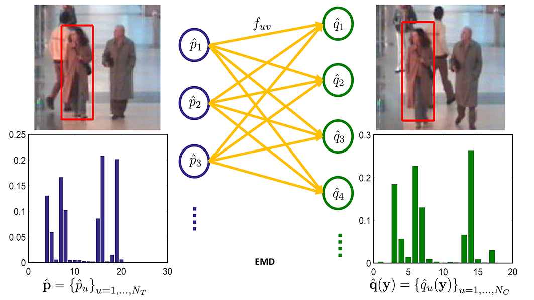
Figure 1: EMD comparison of the two templates.

5.2 EMD as a Function of Weights

Writing the above equation set (2)-(6) in a matrix form as

$$\begin{array}[]{cc}&D^{\star}=\underset{\mathbf{f}}{\mathrm{min\,}}\mathbf{d^{\mathit{T}}}\mathbf{f}\\ \mathrm{s.t.}&\mathbf{H}\mathbf{f}=\mathbf{w};\,\mathbf{f}>0\end{array}$$ (7)

where the $\mathbf{d}=[d_{11},\cdots d_{1N_{C}},\cdots d_{N_{T}1},\cdots d_{N_{T}N_{C}}]^{T}\in\mathbb{R}^{N_{T}N_{C}}$ is the ground distance vector, $\mathbf{f}=[f_{11},\cdots f_{1,N_{C}},\cdots f_{N_{T}1,}\cdots f_{N_{T}N_{C}}]^{T}\in\mathbb{R}^{N_{T}N_{C}}$ is the flow vector, $\mathbf{w}=[\mathbf{w_{\mathit{N_{C}}}^{\mathit{T}}},\mathbf{w}_{N_{T}}^{T}]^{T}\in\mathbb{R}^{N_{T}+N_{C}}$ is the weight vector consisting of the weight vectors $\mathbf{w_{\mathit{N_{C}}}}\in\mathbb{R}^{N_{C}}$ from $\hat{\mathbf{q}}(\mathbf{y})$ and $\mathbf{w_{\mathit{N_{T}}}}\in\mathbb{R}^{N_{T}}$ from $\hat{\mathbf{p}}$, and $\mathbf{H\in\mathbb{R}}^{(N_{T}+N_{C})\times N_{T}N_{C}}$ is the matrix which consists of $0s$ and $1s$.

In order to relate the EMD with the weight vector, the above primal problem in (7) is restated in its dual form as (Dantzig and Thapa, 2006)

$$\begin{array}[]{cc}&D^{\star}=\underset{\mathbf{\pi}}{\mathrm{max}\,}\mathbf{w^{\mathit{T}}}\mathbf{\mathbf{\pi}}\\ \mathrm{s.t.}&\mathbf{H}^{T}\mathbf{\pi}\leq\mathbf{d}\end{array}$$ (8)

where $\pi\in\mathbb{R}^{N_{T}+N_{C}}$ is a vector of variables to be optimized in the dual problem. By solving this dual problem in (8), the optimal solution $D^{\star}$ is calculated and directly represented as the linear equation of weights. However, considering the computation efficiency, the optimal solution (EMD) is first calculated from the primal problem in (7) using the transportation-simplex method, and then the EMD is represented as the function of the weights by the matrix transformation.

Using the transportation-simplex method (Rubner et al., 2000), the optimal solution to the EMD problem in (7) is calculated. The transportation-simplex method is a streamlined simplex algorithm, which is built on the special structure of the transportation problem. In order to reduce the number of iterations of the transportation-simplex method, the Russell’s method is used to compute the initial basic feasible solution (Rubner et al., 2000; Ling and Okada, 2007). The DEMD algorithm (Zhao et al., 2010) uses the standard simplex method to compute the optimal solution to the linear optimization problem in (7). Compared with the standard simplex method, the transportation-simplex method greatly decreases the number of operations (Ling and Okada, 2007). Thus, the iEMD algorithm is more efficient in terms of the number of operations to solve the EMD problem compared with the DEMD algorithm in (Zhao et al., 2010).

The computation of the EMD is a transportation problem, which has exactly $N_{T}+N_{C}-1$ basic variables $\mathbf{f_{\mathit{B}}}\in\mathbb{R}^{N_{T}+N_{C}-1}$, and each constraint is a linear combination of the other $N_{T}+N_{C}-1$ constraints, which could be considered as redundant and discarded (Dantzig and Thapa, 2006). Based on the optimal solution to the linear programming problem, the flow vector is separated into basic variables and non-basic variables as $\mathbf{f}=[\mathbf{f_{\mathit{B}}^{\mathit{T}},\mathbf{\mathbf{f_{\mathit{NB}}^{\mathit{T}}}}}]^{T}\in\mathbb{R}^{N_{T}N_{C}}$, and the ground distance vector $\mathbf{d}$ and $\mathbf{H}$ will be transformed as $\mathbf{d}=[\mathbf{d_{\mathit{B}}^{\mathit{T}},\mathbf{\mathbf{d_{\mathit{NB}}^{\mathit{T}}}}}]^{T}\in\mathbb{R}^{N_{T}N_{C}}$ and $\mathbf{H}=[\mathbf{H_{\mathit{B}},\mathbf{\mathbf{H_{\mathit{NB}}}}}]^{T}\mathbf{\in\mathbb{R}}^{(N_{T}+N_{C})\times N_{T}N_{C}}$, where $\mathbf{d_{\mathit{B}}}\in\mathbb{R}^{N_{T}+N_{C}-1}$, and $\mathbf{H_{\mathit{B}}}\in\mathbb{R}^{(N_{T}+N_{C})\times(N_{T}+N_{C}-1)}$. In order to derive the EMD as a function of the weights of the candidate model, the matrix transformation is performed. First, the last row of the constraint matrices (7) is deleted which is considered as the redundant constraint and then the matrices $\mathbf{H_{\mathit{B}}}$, $\mathbf{H}$, and $\mathbf{w}$ are formulated as $\mathbf{H_{\mathit{B}}^{\ast}}\in\mathbb{R}^{(N_{T}+N_{C}-1)\times(N_{T}+N_{C}-1)}$, $\mathbf{H^{\ast}}=[\mathbf{H_{\mathit{B}}^{\ast},\mathbf{\mathbf{H_{\mathit{NB}}^{\ast}}}}]^{T}\mathbf{\in\mathbb{R}}^{(N_{T}+N_{C}-1)\times N_{T}N_{C}}$ and $\mathbf{w^{\ast}}=[\mathbf{w_{\mathit{N_{C}}}^{\mathit{T}}},\mathbf{w}_{N_{T}-1}^{T}]^{T}\in\mathbb{R}^{N_{T}+N_{C}-1}$.

The problem in (7) is reformulated based on the optimal solution as

$$D^{\star}-\mathbf{d_{B}}^{T}\mathbf{f_{B}}-\mathbf{d_{NB}}^{T}\mathbf{f_{NB}} =0$$ (9)

$$\mathbf{H_{B}^{\ast}}\mathbf{f_{B}}+\mathbf{H_{NB}^{\ast}}\mathbf{f_{NB}} =\mathbf{w^{\ast}}$$ (10)

Left multiplying (10) with $\mathbf{H_{B}^{\ast-1}}$ yields

$$\mathbf{f_{B}}+\mathbf{H_{B}^{\ast-1}\mathbf{H_{NB}^{\ast}}}\mathbf{f_{NB}}=\mathbf{H_{B}^{\ast-1}}\mathbf{w}^{\ast}$$ (11)

Left multiplying (11) by $\mathbf{d_{B}}^{T}$ and adding the resultant to (9) gives

$$D^{\star}+(-\mathbf{d_{NB}}^{T}+\mathbf{M\mathbf{H_{NB}^{\ast}}})\mathbf{f_{NB}}=\mathbf{M}\mathbf{w}^{\ast}$$ (12)

where $\mathbf{M}=\mathbf{d_{B}}^{\mathit{T}}\mathbf{H_{B}^{\ast-1}}$ is a $N_{C}+N_{T}-1$-dimensional vector. Since $\mathbf{f_{NB}}=\mathbf{0}_{N_{T}N_{C}-N_{T}-N_{C}+1}$, using (12) the EMD $D^{\star}$ is given by

$$D^{\star}=\mathbf{M[\mathbf{w_{\mathit{N_{C}}}^{\mathit{T}}},0]_{\mathit{N_{C}+N_{T}-1}}^{\mathit{T}}+M[0,\mathbf{w_{\mathit{N_{T}-1}}^{\mathit{T}}}]_{\mathit{N_{C}+N_{T}-1}}^{\mathit{T}}}$$ (13)

5.3 Gradient Method to Find the Template Displacement

Based on the equation (13) , the gradient method is utilized to find the displacement $\mathbf{y}$ of the target candidate as

$$\frac{\partial D^{\star}}{\partial\mathbf{y}}=\mathbf{M}\left[\mathbf{\frac{\partial w_{\mathit{N_{C}}}^{\mathit{T}}}{\partial y}},0\right]_{N_{C}+N_{T}-1}^{T}$$ (14)

The optimal location $\hat{\mathbf{y}}$ of the template candidate $\hat{\mathbf{q}}(\mathbf{y})$ is found by iteratively performing: (1) calculate the smallest EMD and reformulate it as (13); (2) search for the new location of the template candidate along the direction of (14). When the EMD no longer decreases, the iteration stops. By this method, the best match of the template target and the template candidate will be found. The EMD plays three roles in this algorithm: (1) it provides a metric of the matching between the template target and the template candidate; (2) it assigns more weights to the best matches between the histogram bins and assigns smaller weights or no weights to unmatched bins by linear optimization; (3) matched bins are used for finding the location of the template candidate, and the gradient vector of the EMD for searching the optimal displacement is calculated.

The pseudo-code for the iEMD tracking algorithm is given in Algorithm 1.

1 Set the maximum iteration number ${n_{iter}}$;

2

3Calculate the target model from the image ${I_{0}}$ using (18);

4

5Get the new image frame $I_{k+1}$;

6

7Construct the candidate model from $I_{k+1}$ using (19);

8

9Compute $EMD_{pre}$ between the target model and the candidate model;

10

11for $n$=0 to $n_{iter}$ do

12      

13      Represent the $EMD_{pre}$ by its weight vector $\mathbf{w}^{T}$ using (13);

14      

15      Calculate the derivative of the $EMD$ with respect to the displacement $\mathbf{y}$ using (14);

16      

17      Move the template candidate in $I_{k+1}$ along the gradient vector by one pixel;

18      

19      Compute $EMD$ between the target model and the new candidate model;

20      

21      if $EMD_{pre}<EMD$  then

22             break;

23            

24       end if

25      

26      else

27             n=n+1;

28             Set the $EMD_{pre}=EMD$ ;

29            

30       end if

31      

32 end for

33

34

Algorithm 1 iEMD tracking algorithm

6 Target Modeling Based on Histograms of Sparse Codes

Histogram of sparse codes (HSC) has been widely used as feature descriptors in many fields (Zhang et al., 2013). Given the image set of the first $L$ image templates from a video, a set of $K$ overlapped local image patches are sampled by a sliding window of size $m\times n$ from each template to build a dictionary $\mathbf{\Phi}\in\mathbb{R}^{(mn)\times(LK)}$. Each column of $\mathbf{\Phi}$ is a basis vector, which is a vectorized local image patch extracted from the set of image templates. The basis vectors are overcomplete where $mn<LK$. Similarly, for a given image template target $I$, a set of overlapped local image patches $\mathbf{E}=\left\{\epsilon_{r}|\epsilon_{r}\in\mathbb{R}^{(mn)\times 1},r=1\cdots J\right\}$ are sampled by the same sliding window of size $m\times n$ with the step size of one pixel. Each image patch $\epsilon_{r}$, which represents one fixed part of the target object, can be encoded as a linear combination of a few basis vectors of the dictionary $\mathbf{\Phi}$ as follows

$$\epsilon_{r}=\mathbf{\Phi}\mathbf{a}_{r}+\mathbf{n}$$ (15)

where $\mathbf{a}_{r}\in\mathbb{R}^{(LK)\times 1}$ is the coefficient vector which is sparse and $\mathbf{n}\in\mathbb{R}^{(mn)\times 1}$ is the noise vector. The coefficient $\mathbf{a}_{r}$ is computed by solving the following $L_{1}$ norm minimization problem (Zhang et al., 2013; Mairal et al., 2014)

$$\begin{array}[]{cc}\underset{\mathbf{a}_{r}}{\mathbf{\mathrm{min}}}&\left\|\epsilon_{r}-\mathbf{\Phi}\mathbf{a}_{r}\right\|_{2}^{2}+\lambda\left\|\mathbf{a}_{r}\right\|_{1}\\ \mathrm{s.t.}&(\mathbf{a}_{r})_{k}\geq 0,\forall k\end{array}$$ (16)

where $\mathbf{a}_{r}=\left[\begin{array}[]{ccccccc}a_{11},&\cdots,&a_{1K},&\cdots,&a_{L1},&\cdots,&a_{LK}\end{array}\right]^{T}$ is the sparse coefficients of the local patch, $a_{ij}$ corresponds to the $\mathrm{\mathit{j}\mathrm{th}}$ patch of the $i\mathrm{\mathrm{th}}$ image template of the dictionary, and $\lambda$ is the Lagrange multiplier.

Once a solution to (16) is obtained, the maximum-alignment-pooling method is used to construct the sparse coding histograms. Combining the coefficients corresponding to the dictionary patches that have the same locations in the template using $\bar{a}_{j}=\sum_{i=1}^{L}a_{ij}$ (Jia et al., 2016), a new vector $\bar{\mathbf{a}}_{r}=[\begin{array}[]{ccc}\bar{a}_{1},&\cdots,&\bar{a}_{j}\end{array}]^{T}\in\mathbb{R}^{K\times 1}$ is formulated. The weight of the $r\mathrm{th}$ local image patch $\epsilon_{r}$ in the histogram of sparse codes is computed by using $\hat{p}_{ru}=\left\|\bar{\mathbf{a}}_{r}\right\|_{\infty}$. The $\hat{p}_{ru}$ value corresponds to the $u\mathrm{th}$ image patch from $\bar{\mathbf{a}}_{r}$. With $J$ local image patches from the template target, the histogram is constructed as

$$\hat{\mathbf{p}}=[\begin{array}[]{c}\hat{p}_{11},\cdots,\hat{p}_{ru},\cdots,\hat{p}_{JK}\end{array}]^{T}\in\mathbb{R}^{J\times 1}$$ (17)

In the spatial space, the Epanechnikov kernel is used to represent the template. The Epanechnikov kernel (Comaniciu et al., 2003) is an isotropic kernel with a convex profile which assigns smaller weights to pixels away from the center. Given the target histogram $\hat{\mathbf{p}}$ in (17), the isotropic kernel is applied to generate the histograms of target weighted by the spatial locations. The weights of the histogram of the target $w_{T,u}$ are computed using

$$w_{T,u}=\gamma\sum_{r=1}^{J}\left(1-\left\|\frac{\mathbf{c}_{r}}{h}\right\|^{2}\right)\left|\hat{p}_{ru}\right|$$ (18)

where $\mathbf{c}_{r}$ is the center of the $r\mathrm{th}$ image patch of the template target, $h$ is template size and $\gamma$ is the normalization constant. The candidate histogram $\hat{\mathbf{q}}$ is built in the same way as $\hat{\mathbf{p}}$. An isotropic kernel is applied to the elements of the $\hat{\mathbf{q}}$ for generating the histogram of candidate with spatial locations. The weights of the candidate histogram $w_{C,v}(\mathbf{x_{\mathit{i}}-\mathbf{y}})$ are computed using

$$w_{C,v}(\mathbf{x_{\mathit{i}}-\mathbf{y}})=\gamma\sum_{r=1}^{J}\left(1-\left\|\frac{\mathbf{c}_{r}-\mathbf{y}}{h}\right\|^{2}\right)\left|\hat{q}_{rv}\right|$$ (19)

where $\mathbf{y}$ is the displacement of the $r\mathrm{th}$ image patch of the template candidate. The ground distance $d_{uv}$ for the EMD in (2) is defined by

$$d_{uv}=\alpha\left\|\mathbf{\epsilon}_{u}-\mathbf{\epsilon}_{v}\right\|_{2}^{2}+(1-\alpha)\left\|\mathbf{c}_{u}-\mathbf{c}_{v}\right\|_{2}^{2}$$ (20)

where $\alpha\in\left(0,1\right)$ is the weighting coefficient, $\mathbf{\epsilon}_{u}\in\mathbb{R}^{(mn)\times 1}$, $\mathbf{\epsilon}_{v}\in\mathbb{R}^{(mn)\times 1}$ are the vectors of the normalized pixel values of the image patch from the target and candidate templates, sampled in the same way as the image patches from the dictionary, and $\mathbf{c}_{u}$, $\mathbf{c}_{v}$ are the corresponding centers of the image patches.

7 Extensions of The Tracking Algorithm

7.1 Template Update

In order to make the tracker robust to significant appearance variations during long video sequences, the outdated templates in the dictionary should be replaced with the recent ones. To adapt to the appearance variations of the target and alleviate the drift problem only the latest template in dictionary is replaced based on the weight $\omega_{i}$, which is computed by

$$\omega_{i}=\gamma_{0}^{\varDelta i}\times\exp(-D_{k}^{*})$$ (21)

where $\omega_{i}$ is the weight associated with the template, $\gamma_{0}$ is a constant, $\varDelta i$ is the time elapsed since the dictionary was last updated measured in terms of image index $k$ and $D_{k}^{*}$ is the EMD value corresponding to the template $I_{k}$.

If the weight of the current template based on (21) is smaller than the weight of the latest template in the dictionary, the template is replaced with the current one. In order to avoid the errors and noises affecting the dictionary update algorithm, the reconstructed template is used to replace the one in the dictionary. Firstly, the following problem is solved in order to recompute the sparse code coefficients, $\mathbf{a}_{k}$,

$$\underset{\mathbf{a}_{k}}{\mathbf{\mathrm{min}}}\left\|I_{k}-[\begin{array}[]{cc}\mathbf{\Phi_{\mathrm{T}}}&\mathbf{I}_{mn\times mn}\end{array}]\mathbf{a}_{k}\right\|_{2}^{2}+\lambda\left\|\mathbf{a}_{k}\right\|_{1}$$ (22)

where $\mathbf{\Phi_{\mathrm{T}}\in\mathbb{R}}^{(mn)\times K}$ is a dictionary formed using the vectorized template image with the size $m\times n$ as columns, $\mathbf{I}_{mn\times mn}$ is the identity matrix, $\mathbf{a}_{k}\in\mathbb{R}^{K+mn}$ is the vector of the sparse coding coefficients, and $\lambda$ is the Lagrange multiplier (cf., (Jia et al., 2016)). Then the reconstructed template is calculated using $\mathbf{\Phi_{\mathrm{T}}}\mathbf{a}_{k}^{*}$, where $\mbox{$\mathbf{a}$}_{k}^{*}\in\mathbb{R}^{K}$ is computed using components of $\mathbf{a}_{k}$ corresponding to the dictionary. The reconstructed template is used to replace the latest template in the dictionary. The detailed steps of the update scheme are given in Algorithm 2.

1

2

Input : The tracked template $I_{k}$ and the EMD value $D_{k}^{*}$ at frame $k$, the current dictionary $\Phi_{i-1}=\left[\begin{array}[]{cccc}\mathbf{d}_{1},&\mathbf{d}_{2},&\cdots,&\mathbf{d}_{K}\end{array}\right]$ at index $i-1$, and the associated weights of the latest template in dictionary $\omega_{i-1}$.

3

Output : The updated dictionary $\Phi_{i}$ and weights $\omega_{i}$.

4

5Compute the weight of the current template using $\omega_{i}=\exp(-D_{k}^{*})$;

6

7Update $\omega_{i-1}$ via (21);

8

9if $\omega_{i}<\omega_{i-1}$  then

10      

11      $\omega_{i-1}\leftarrow\omega_{i}$;

12      

13      Calculate the reconstructed template via (22);

14      

15      $\mathbf{d}_{K}\leftarrow\mathbf{\Phi_{\mathrm{T}}}\mathbf{a}_{k}^{*}$;

16      

17 end if

18

Algorithm 2 Template update procedure.

7.2 Gyroscope Data Fusion for Rotation Compensation

The general idea of the gyro-aided iEMD tracking algorithm is combining the image frames from the camera with the angular rate generated by the gyroscope for visual tracking. Synchronization of the camera and the gyroscope in time is required. The spatial relationship between the camera and the gyroscope must also be pre-calibrated. Then, the angular rate generated by the gyroscope is applied to compensate for the ego-motion of the camera. After the compensation of the ego-motion of the camera, the iEMD tracker is applied for tracking. In this section, the gyro-aided iEMD tracking algorithm is developed and illustrated.

When a camera is mounted on a moving robot, the motion of the camera will cause a large displacement of the target between two consecutive frames. If the displacement is larger than the convergence region, the tracking algorithm will become susceptible to the large appearance changes and fail (Comaniciu et al., 2003; Hwangbo et al., 2011; Ravichandar and Dani, 2014). In order to improve the robustness of the tracking algorithm, the displacement caused by the camera rotation is estimated and compensated by fusing the data from the gyroscope, which is a commonly used sensor on flying robots. The rotation of the camera causes a larger displacement of the target compared with the translation movement in video-rate frames. Thus, the translation is neglected here.

The gyroscope provides the angular rate along three axes, which measure the pan, tilt, and roll of small time intervals $\varDelta t$. In the case of pure rotation without translation, the angular rate $\omega_{y}$ is obtained along three axes $x$, $y$ and $z$. Let $q(k),\,q(k+1)\in\mathbb{H}$ denote the quaternion of two frames $k$ and $k+1$ during time $\varDelta t$, the relationship between them is given as (cf. (Spong et al., 2006))

$$q(k+1)=q(k)+\frac{1}{2}\Omega(\omega)\cdot q(k)\cdot\varDelta t$$ (23)

where $\Omega(\omega)$ is the skew-symmetric matrix of $\omega$ as

$$\Omega(\omega)=\left[\begin{array}[]{cc}0&-\omega^{T}\\ \omega&-[\omega]_{\times}\end{array}\right]$$ (24)

After the quaternion $q(k+1)=m+a\mathbf{i}+b\mathbf{j}+c\mathbf{k}$ is normalized and updated, the rotation matrix $R_{k}^{k+1}$ is calculated as

$$R_{k}^{k+1}=\left[\begin{array}[]{ccc}1-2b^{2}-2c^{2}&2ab-2cm&2ac+2bm\\ 2ab+2cm&1-2a^{2}-2c^{2}&2bc-2am\\ 2ac-2bm&2bc+2am&1-2a^{2}-2b^{2}\end{array}\right]$$ (25)

Thus, the estimated homography matrix between two templates is estimated by

$$\mathbb{\mathcal{H}}_{\mathrm{gyro}}=KR_{k}^{k+1}K^{-1}$$ (26)

where, $K$ is the intrinsic camera calibration matrix that is accessed by calibrating the camera. The homography matrix is updated to the newest frame location $p(k+1)=[x_{c},y_{c},1]^{T}$, where $(x_{c},y_{c})$ is the center point of the template, based on the following equations:

$$\mathbb{\mathcal{H}}^{k+1}=\mathbb{\mathcal{H}}^{k}\mathbb{\mathcal{\ H}}_{\mathrm{gyro}}^{-1}$$ (27)

$$p(k+1)=\mathbb{\mathcal{H}}^{k+1}\cdot p(k)$$ (28)

for the first frame, $\mathbb{\mathcal{H}}^{0}=\mathbf{I}_{3\times 3}$. This new location $p(k+1)=[x_{c},y_{c},1]^{T}$ is then used as the initial guess of the object candidate and the probability of the tracking algorithm to find the location of the object target in the new video frame is improved.

The pseudo-code for gyro-aided iEMD algorithm is given in Algorithm 3.

1 Set the maximum iteration number ${n_{iter}}$, ${n_{scal}}$;

2Capture the image ${I_{0}}$;

3 if $t=0$ then

4       Display the first image ${I_{t}}$ ;

5       Request user to select template to be tracked ;

6      

7      Construct the target model from the template;

8      

9 end if

10

11while tracking do

12       Capture the image $I_{t+1}$;

13       Obtain the angular rate from gyroscope;

14       Integrate angular rates to obtain inter-frame rotation, $R_{t}^{t+1}$ using (25);

15       Compute 2D homography $\mathbb{\mathcal{H}}_{\mathrm{gyro}}$ using (26);

16       Initialize the location of the template using (28);

17       Track the target by the iEMD tracking algorithm from Algorithm 1

18 end while

19

Algorithm 3 Gyro-aided iEMD tracking algorithm

8 Experiments

In this section, the iEMD algorithm is validated on real datasets. The algorithm is implemented by MATLAB R2015b, the C code in (Rubner et al., 2000) is adopted for the EMD calculation, and the software in (Mairal et al., 2014) is used for sparse modeling. The platform is Microsoft Windows 7 professional with Intel(R) Core(TM) i5-4590 CPU. Eight publicly available datasets are chosen to validate the iEMD tracking algorithm. The main attributes of the video sequences are summarized in Table 1. The Car2, Walking, Woman, Subway, Bolt2, Car4, Human8, and Walking2 sequences are from the visual tracker benchmark (Wu et al., 2013) (CVPR 2013, http://www.visual-tracking.net). The length of the sequences varies between 128 and 913 frames with one object being tracked in each frame.

The tracker is initialized with the ground-truth bounding box of the target in the first frame. Then the tracking algorithm runs till the end of the sequence and generates a series of the tracked bounding boxes. Tracking results from consecutive frames are compared with the ground truth bounding boxes provided by this dataset. The relative overlap measure is used to evaluate this algorithm as (Wu et al., 2013)

$$\mathrm{overlap}=\frac{\mathbf{R}_{tr}\cap\mathbf{R}_{gt}}{\mathbf{R}_{tr}\cup\mathbf{R}_{gt}}$$ (29)

where $\mathbf{R}_{tr}$ is the tracking result, represented by the estimated image region occupied by the tracked object, $\mathbf{R}_{gt}$ is the ground truth bounding box. $\mathbf{R}_{tr}\cap\mathbf{R}_{gt}$ is the intersection and $\mathbf{R}_{tr}\cup\mathbf{R}_{gt}$ is the union of the two regions. The range of the relative overlap is from $0$ to $100\%$ .

8.1 Results for the iEMD tracker with sparse coding histograms

In this subsection, the performance of the iEMD tracker with sparse coding histograms and the template update method is evaluated using the eight sequences. In our approach, the object windows are re-sized to $32\times 32$ pixels for all the sequences, except for the Walking sequence, in which the object windows are resized to $64\times 32$ pixels due to the smaller object size. The local patches in each object window are sampled with the size $16\times 16$ pixels with step size $8$ in sequences like Car4, Walking and Car2. For other sequences, the local patches in each object window are sampled with the size $8\times 8$ pixels with step size $4$. In the case of the abrupt motions of the object, $4$ more particles are generated by moving the template in the surrounding area of the initial object position. For each particle, the template is enlarged and shrunk by $2\%$ in case of the scale variations.

Table 1: The main attributes of the video sequences. Target size: the initial target size in the first frame, IV: illumination variation, SV: scale variation, OCC: occlusion, DEF: deformation, MB: motion blur, FM: fast motion, BC: background clutters.

Sequence	Frames	Image size	Target size	IV	SV	OCC	DEF	MB	FM	BC
Car4	$659$	$360\times 240$	$107\times 87$	$\checked$	$\checked$
Walking	$412$	$768\times 576$	$24\times 79$		$\checked$	$\checked$	$\checked$
Woman	$550$	$352\times 288$	$21\times 95$	$\checked$	$\checked$	$\checked$	$\checked$	$\checked$	$\checked$
Subway	$175$	$352\times 288$	$19\times 51$			$\checked$	$\checked$			$\checked$
Bolt2	$293$	$480\times 270$	$34\times 64$				$\checked$			$\checked$
Car2	$913$	$320\times 240$	$64\times 52$	$\checked$	$\checked$			$\checked$	$\checked$	$\checked$
Human8	$128$	$320\times 240$	$30\times 91$	$\checked$	$\checked$		$\checked$
Walking2	$500$	$384\times 288$	$31\times 115$		$\checked$	$\checked$

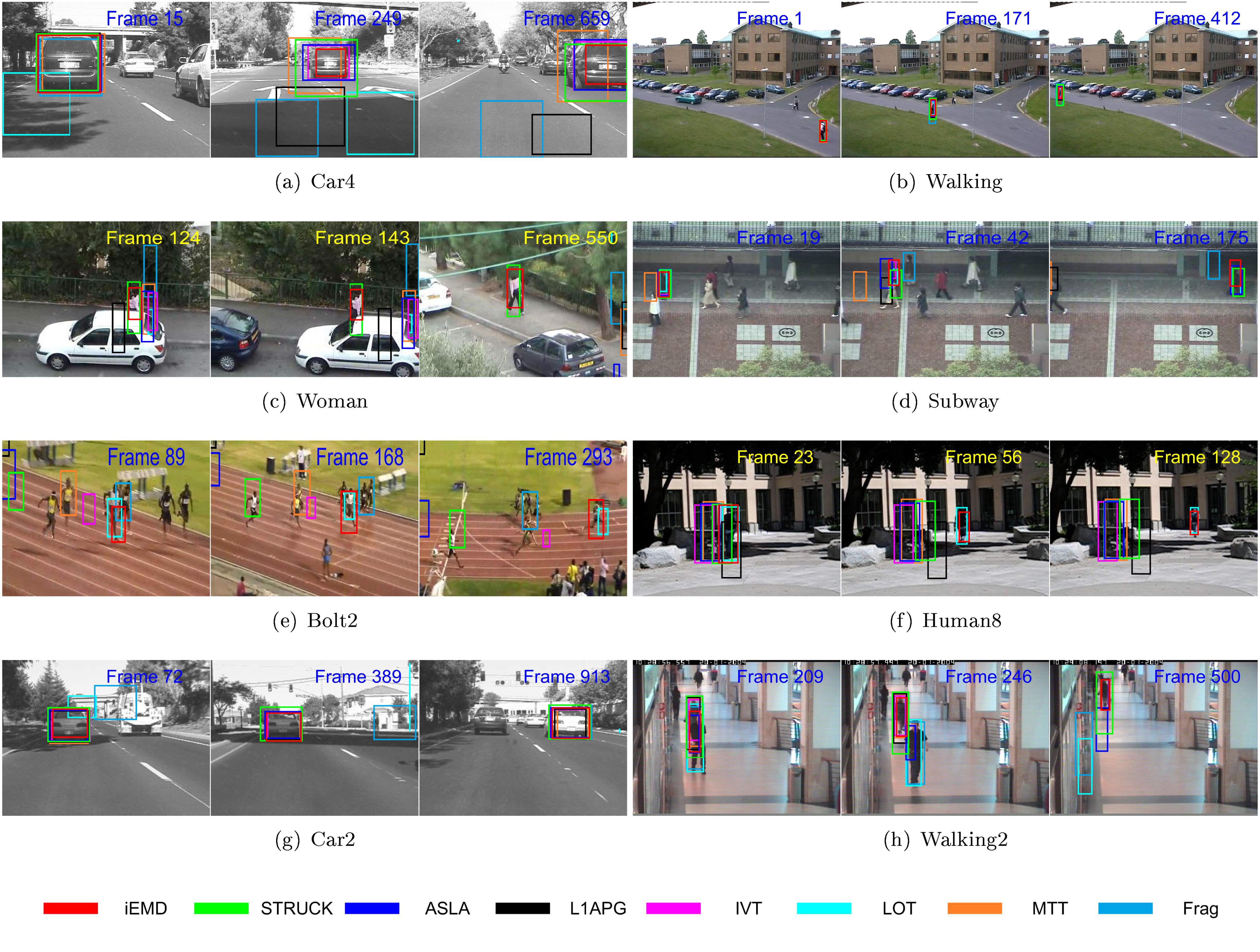
Figure 2: The visual tracking results obtained by the eight tracking algorithms on the eight video sequences.

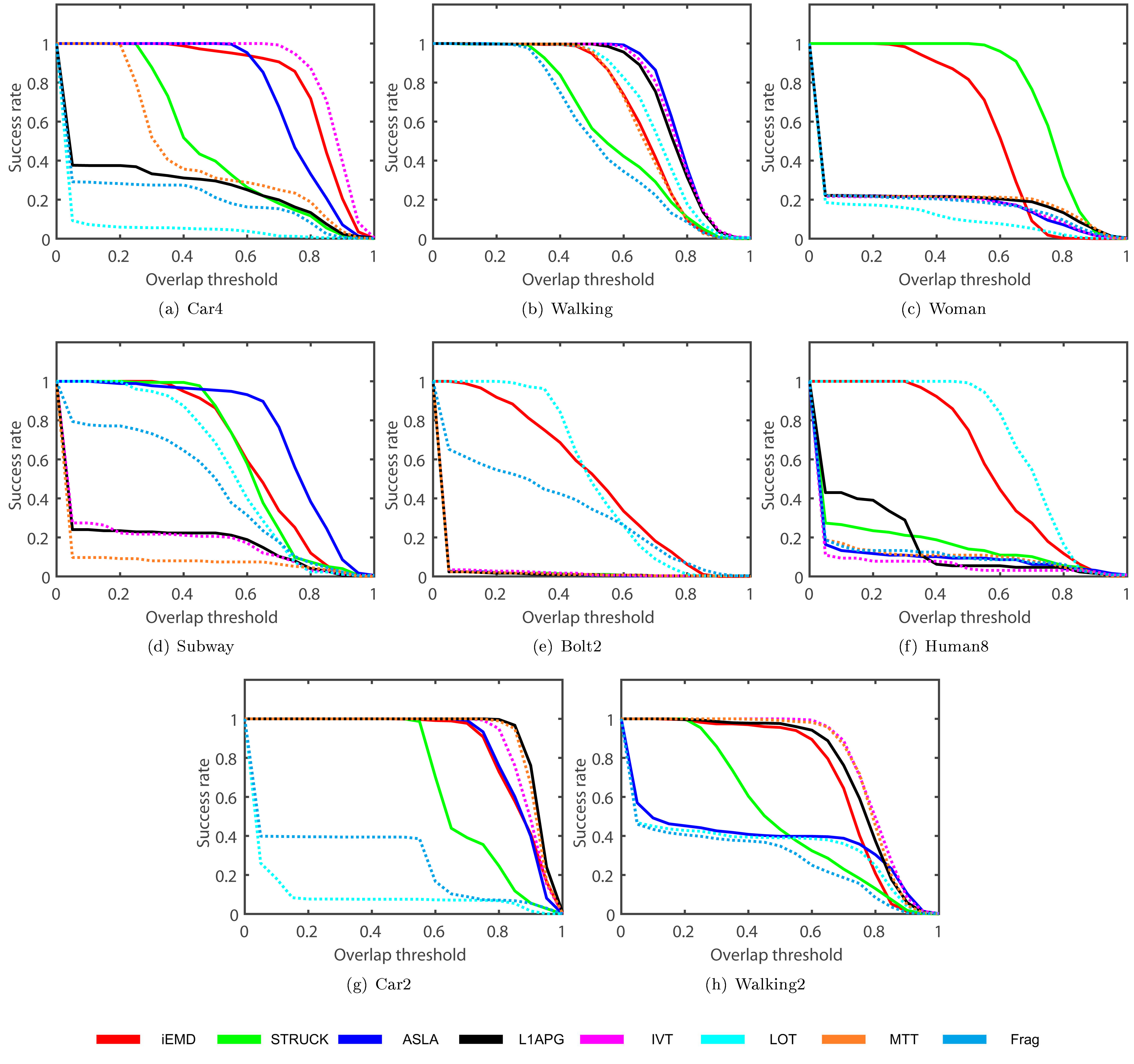
Figure 3: Success plots ((a)-(j)) for the eight tracking algorithms on the eight sequences.

The performance of the proposed algorithm is compared with seven state-of-the-art tracking algorithms on eight video sequences. These state-of-the-art trackers include: ASLA (Jia et al., 2012), Frag (Adam et al., 2006), IVT (Ross et al., 2008), L1APG (Mei and Ling, 2011), LOT (Oron et al., 2012), MTT (Zhang et al., 2012), and STRUCK (Hare et al., 2011). The source codes of the trackers are downloaded from the corresponding web pages and the default parameters are used. The average percentage overlap obtained by all the tracking algorithms on eight video sequences are reported in Table 2. The iEMD tracker achieves the highest average overlap over all the sequences. The iEMD tracker also achieves the second best tracking results on the 5 out of $8$ sequences. In Fig. LABEL:fig:Sucess-plots,_the_success_plots_obtained_by_all_the_tracking_algorithms_oneight video sequences are shown. The success plot shows the ratios of frames at the different thresholds of the relative overlap values varied from $0$ to $1$.

Table 2: The average overlap (in percentage) obtained by the tracking algorithms on eight datasets. For each sequence, the first, second and third ranks are marked in red, green and blue respectively. The last row is the average value of the percentage overlap for each tracker over all sequences.

Sequence	ASLA	Frag	IVT	L1APG	LOT	MTT	STRUCK	iEMD
Car4	75.4	18.8	87.6	24.9	4.2	44.7	48.9	82.0
Walking	77.2	53.7	76.6	75.3	70.4	66.6	57.1	67.1
Woman	14.8	14.7	14.7	16.2	8.9	16.7	73.2	60.7
Subway	75.6	44.0	15.9	16.2	56.0	6.8	62.6	63.9
Bolt2	1.1	32.6	1.6	1.1	51.8	1.1	1.2	50.1
Car2	86.4	25.9	89.3	92.4	8.6	91.5	68.8	86.2
Human8	8.8	9.7	5.5	15.6	70.4	9.8	14.7	60.2
Walking2	37.1	27.4	79.5	75.6	33.5	78.5	51.0	71.2
Average	47.1	28.4	46.3	39.7	38.0	39.5	47.2	67.7

Representative tracking results obtained by iEMD algorithm are shown in Fig. 2. In the Human8 and Bolt2 sequences, the targets have significant illumination variations, and deformations, respectively. Only LOT and iEMD trackers are able to track the target in all the frames. Both of them use the EMD as the similarity measure and their appearance models are based on local image patches, which make the trackers more robust to illumination changes and deformations (Oron et al., 2012; Rubner et al., 2000). In woman sequence, all the trackers start to drift away from the target in frame $124$ except for the iEMD and STRUCK trackers. For the Car2 and Car4 sequences, there are significant illumination changes when the targets pass underneath the trees and the overpasses. The LOT and Frag trackers start drifting away from frame $72$ in Car2 sequences. In Car4 sequence, the LOT tracker starts to lose the target from frame $15$, and the Frag and L1APG trackers drift away when the car passes the overpass in frame $249$. In Walking2 sequence, the LOT, Frag, and ASLA trackers start tracking the wrong target in frame $246$, due to the similar colors of the clothes between the two people.

8.2 Results for the Gyro-aided iEMD tracking algorithm

The test of the gyro-aided iEMD tracking algorithm is conducted using the sequence including 100 frames from the dataset provided by CMU (Hwangbo et al., 2011). The size of the template is changed by $\pm 10\%$ and the template with the best scale is found, giving the smallest $EMD$. The images are taken in front of a desk with motions, such as shaking and rotation. The frame sequences have a resolution of $640\times 480$ at $30\mathrm{FPS}$. The gyroscope is carefully aligned with the camera and the tri-axial gyroscopic values are sampled at $11\mathrm{Hz}$ in the range of $\pm 200\mathrm{deg/sec}$ (Hwangbo et al., 2011). Using the time stamps of the camera and the gyroscope, the angular rate data are synchronized with the frames captured by the camera.

The comparisons between the tracking results using the iEMD tracker with and without the gyroscope information are illustrated in Fig. 4. The head of the eagle is chosen as the target and the ground truth is manually labeled in each frame. The magenta box indicates the estimated image region without using the gyroscope data, and the cyan box is the tracking results of the gyro-aided iEMD tracker. Without the gyroscope data, the tracker loses the target after the frame $25$. However, the head of the eagle is successfully tracked with our gyro-aided iEMD tracking algorithm.

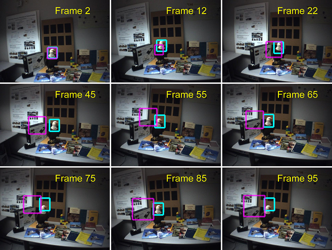
Figure 4: Results of the iEMD tracker in presence of rapid camera motion; the magenta boxes indicate the results of the iEMD tracker without the gyroscope information, and the cyan boxes indicate the results of the gyro-aided iEMD tracker.

The performances of the iEMD tracker with and without the gyroscope information on the CMU sequence are summarized in Table 3. The value of the average overlap, the percentage of the total frame numbers of which the overlap is greater than $0$ and $40\%$ are reported. Gyroscope information provides a good initial position for the iEMD tracker to estimate the location of the target. Thus, the gyro-aided iEMD tracking algorithm is robust to the rapid movements of the camera.

Table 3: Evaluation results on the CMU dataset using the iEMD tracker with and without the gyroscope information.

Relative overlap with the ground truth	Gyro-aided	No gyro-aided
Average overlap (%)	$50.7$	$11.9$
Overlap $>0$	$100$	$70.7$
Overlap $>40\%$	$66.7$	$9.1$

8.3 Discussion

As a cross-bin metric for the comparison of the histograms, the advantages of the EMD are demonstrated in situations such as illumination variation, object deformation and partial occlusion. The iEMD algorithm uses the transportation-simplex algorithm for calculating the EMD in the experiments, of which the practical running time complexity is the supercubic (a complexity in $\Omega(N^{3})\bigcap O(N^{4})$) (Rubner et al., 2000), where $N$ represents the number of the histogram bins. Other algorithms for calculating the EMD can be used to further shorten the running time (Ling and Okada, 2007; Pele and Werman, 2009). The experimental results, especially the Human8 and Bolt2 sequences, show that the iEMD tracker is robust to the appearance variations. The experimental results of Walking2 shows that the iEMD tracker can discriminate the target from the surroundings with similar colors. The tracking results from Woman and Subway sequences demonstrate the robustness to partial occlusions. Since the local sparse representation is adopted as the appearance model, the methods such as the trivial templates, learning dictionary from the target and background images, could be adopted to improve the performance of iEMD tracker. As a gradient descent based dynamic model, the iEMD tracker, which provides good location prediction, can be further improved with more effective particle filters. The metrics used by sparse coding, such as the largest sum of the sparse coefficients or the smallest reconstruction error, can be combined with the EMD to make the tracker more discriminant.

9 Conclusion

This paper presents iEMD and gyro-aided iEMD visual tracking algorithms. The local sparse representation is used as the appearance model for the iEMD tracker. The maximum-alignment-pooling method is used for constructing a sparse coding histogram which reduces the computational complexity of the EMD optimization. The template update algorithm based on the EMD is also presented. The iEMD tracker is robust to variations in appearance of the target, deformations and partial occlusions. Experiments conducted on eight publicly available datasets show that the iEMD tracker is robust to the illumination changes, deformations and partial occlusions of the target. To validate the gyro-aided iEMD tracking algorithm, experimental results from the CMU dataset, which contains rapid camera motion are presented. Without the gyroscope measurements, the iEMD tracker fails on the CMU dataset. With the help of the gyroscope measurements, the iEMD algorithm is able to lock onto the target and track it successfully. The above experimental results show that the proposed iEMD tracking algorithm is robust to the appearance changes of the target as well as the ego-motion of the camera.

References

- Adam et al. (2006) Adam, A., Rivlin, E., and Shimshoni, I. (2006). Robust fragments-based tracking using the integral histogram. In IEEE Computer Society Conf. on Computer Vision and Pattern Recognition. 798–805
- Avidan (2007) Avidan, S. (2007). Ensemble tracking. IEEE Trans. on Pattern Analysis and Machine Intelligence 29, 261–271
- Babenko et al. (2011) Babenko, B., Yang, M.-H., and Belongie, S. (2011). Robust object tracking with online multiple instance learning. IEEE Trans. on Pattern Analysis and Machine Intelligence 33, 1619–1632
- Baum et al. (2015) Baum, M., Willett, P., and Hanebeck, U. D. (2015). On Wasserstein Barycenters and MMOSPA estimation. IEEE Signal Processing Letters 22, 1511–1515
- Bolme et al. (2010) Bolme, D. S., Beveridge, J. R., Draper, B. A., and Lui, Y. M. (2010). Visual object tracking using adaptive correlation filters. In IEEE Conf. on Computer Vision and Pattern Recognition. 2544–2550
- Chwa et al. (2016) Chwa, D., Dani, A. P., and Dixon, W. E. (2016). Range and motion estimation of a monocular camera using static and moving objects. IEEE Trans. on Control Systems Technology , 1–10
- Collins et al. (2005) Collins, R. T., Liu, Y., and Leordeanu, M. (2005). Online selection of discriminative tracking features. IEEE Trans. on Pattern Analysis and Machine Intelligence 27, 1631–1643
- Comaniciu et al. (2003) Comaniciu, D., Ramesh, V., and Meer, P. (2003). Kernel-based object tracking. IEEE Trans. on Pattern Analysis and Machine Intelligence 25, 564–577
- Dani et al. (2012) Dani, A. P., Fischer, N. R., and Dixon, W. E. (2012). Single camera structure and motion. IEEE Trans. on Automatic Control 57, 238–243
- Dani et al. (2013) Dani, A. P., Panahandeh, G., Chung, S.-J., and Hutchinson, S. (2013). Image moments for higher-level feature based navigation. In IEEE/RSJ Int’l Conf. on Intelligent Robots and Systems. 602–609
- Dantzig and Thapa (2006) Dantzig, G. B. and Thapa, M. N. (2006). Linear programming 1: Introduction (Springer Science & Business Media)
- Davison et al. (2007) Davison, A. J., Reid, I. D., Molton, N. D., and Stasse, O. (2007). MonoSLAM: Real-time single camera SLAM. IEEE Trans. on Pattern Analysis and Machine Intelligence 29, 1052–1067
- Grabner and Bischof (2006) Grabner, H. and Bischof, H. (2006). On-line boosting and vision. In IEEE Computer Society Conf. on Computer Vision and Pattern Recognition. 260–267
- Guerriero et al. (2010) Guerriero, M., Svensson, L., Svensson, D., and Willett, P. (2010). Shooting two birds with two bullets: how to find Minimum Mean OSPA estimates. In Int’l Conf. on Information Fusion. 1–8
- Hare et al. (2011) Hare, S., Saffari, A., and Torr, P. H. (2011). STRUCK: Structured output tracking with kernels. In Int’l Conf. on Computer Vision. 263–270
- Hwangbo et al. (2011) Hwangbo, M., Kim, J.-S., and Kanade, T. (2011). Gyro-aided feature tracking for a moving camera: fusion, auto-calibration and GPU implementation. Int’l J. of Robotics Res. 30, 1755–1774
- Jia et al. (2012) Jia, X., Lu, H., and Yang, M.-H. (2012). Visual tracking via adaptive structural local sparse appearance model. In IEEE Conf. on Computer vision and pattern recognition. 1822–1829
- Jia et al. (2016) Jia, X., Lu, H., and Yang, M.-H. (2016). Visual tracking via coarse and fine structural local sparse appearance models. IEEE Trans. on Image Processing 25, 4555–4564
- Kalal et al. (2012) Kalal, Z., Mikolajczyk, K., and Matas, J. (2012). Tracking-learning-detection. IEEE Trans. on Pattern Analysis and Machine Intelligence 34, 1409–1422
- Karavasilis et al. (2011) Karavasilis, V., Nikou, C., and Likas, A. (2011). Visual tracking using the earth mover’s distance between gaussian mixtures and Kalman filtering. Image and Vision Computing 29, 295–305
- Li et al. (2016) Li, H., Li, Y., and Porikli, F. (2016). Convolutional neural net bagging for online visual tracking. Computer Vision and Image Understanding 153, 120–129
- Ling and Okada (2007) Ling, H. and Okada, K. (2007). An efficient earth mover’s distance algorithm for robust histogram comparison. IEEE Trans. on Pattern Analysis and Machine Intelligence 29, 840–853
- Liu et al. (2011) Liu, B., Huang, J., Yang, L., and Kulikowsk, C. (2011). Robust tracking using local sparse appearance model and K-selection. In IEEE Conf. on Computer Vision and Pattern Recognition. 1313–1320
- Mairal et al. (2014) Mairal, J., Bach, F., Ponce, J., et al. (2014). Sparse modeling for image and vision processing. Foundations and Trends® in Computer Graphics and Vision 8, 85–283
- Mei and Ling (2009) Mei, X. and Ling, H. (2009). Robust visual tracking using L1 minimization. In IEEE 12th Int’l Conf. on Computer Vision. 1436–1443
- Mei and Ling (2011) Mei, X. and Ling, H. (2011). Robust visual tracking and vehicle classification via sparse representation. IEEE Trans. on Pattern Analysis and Machine Intelligence 33, 2259–2272
- Oron et al. (2012) Oron, S., Bar-Hillel, A., Levi, D., and Avidan, S. (2012). Locally orderless tracking. In IEEE Conf. on Computer Vision and Pattern Recognition. 1940–1947
- Park et al. (2013) Park, J., Hwang, W., Kwon, H., Kim, K., et al. (2013). A novel line of sight control system for a robot vision tracking system, using vision feedback and motion-disturbance feedforward compensation. Robotica 31, 99–112
- Pele and Werman (2009) Pele, O. and Werman, M. (2009). Fast and robust earth mover’s distances. In IEEE Int’l Conf. on Computer vision. 460–467
- Ravichandar and Dani (2014) Ravichandar, H. C. and Dani, A. P. (2014). Gyro-aided image-based tracking using mutual information optimization and user inputs. In IEEE Int’l Conf. on Systems, Man and Cybernetics. 858–863
- Ravichandar and Dani (2015) Ravichandar, H. C. and Dani, A. P. (2015). Human intention inference through interacting multiple model filtering. In IEEE Conf. on Multisensor Fusion and Integration
- Ross et al. (2008) Ross, D. A., Lim, J., Lin, R.-S., and Yang, M.-H. (2008). Incremental learning for robust visual tracking. Int’l J. of Computer Vision 77, 125–141
- Rubner et al. (2000) Rubner, Y., Tomasi, C., and Guibas, L. J. (2000). The earth mover’s distance as a metric for image retrieval. Int’l J. of Computer Vision 40, 99–121
- Santner et al. (2010) Santner, J., Leistner, C., Saffari, A., Pock, T., and Bischof, H. (2010). Prost: Parallel robust online simple tracking. In IEEE Conf. on Computer Vision and Pattern Recognition. 723–730
- Spong et al. (2006) Spong, M. W., Hutchinson, S., and Vidyasagar, M. (2006). Robot modeling and control, vol. 3 (Wiley New York)
- Vojir et al. (2016) Vojir, T., Matas, J., and Noskova, J. (2016). Online adaptive hidden markov model for multi-tracker fusion. Computer Vision and Image Understanding 153, 109–119
- Wang et al. (2015) Wang, J., Wang, H., and Zhao, W.-L. (2015). Affine hull based target representation for visual tracking. J. of Visual Communication and Image Representation 30, 266–276
- Wang et al. (2016) Wang, J., Wang, Y., and Wang, H. (2016). Adaptive appearance modeling with Point-to-Set metric learning for visual tracking. IEEE Trans. on Circuits and Systems for Video Technology 10.1109/TCSVT.2016.2556438
- Wu et al. (2013) Wu, Y., Lim, J., and Yang, M.-H. (2013). Online object tracking: A benchmark. In IEEE Conf. on Computer Vision and Pattern Recognition (CVPR)
- Yang et al. (2015) Yang, J., Dani, A. P., Chung, S.-J., and Hutchinson, S. (2015). Vision-based localization and robot-centric mapping in riverine environments. J. of Field Robotics 10.1002/rob.21606
- Yilmaz et al. (2006) Yilmaz, A., Javed, O., and Shah, M. (2006). Object tracking: A survey. ACM Computing Surveys 38, 13
- Zhang et al. (2013) Zhang, S., Yao, H., Sun, X., and Lu, X. (2013). Sparse coding based visual tracking: Review and experimental comparison. Pattern Recognition 46, 1772–1788
- Zhang et al. (2012) Zhang, T., Ghanem, B., Liu, S., and Ahuja, N. (2012). Robust visual tracking via multi-task sparse learning. In IEEE Conf. on Computer Vision and Pattern Recognition. 2042–2049
- Zhang and Hong Wong (2014) Zhang, Z. and Hong Wong, K. (2014). Pyramid-based visual tracking using sparsity represented mean transform. In Proc. of the IEEE Conf. on Computer Vision and Pattern Recognition. 1226–1233
- Zhao et al. (2010) Zhao, Q., Yang, Z., and Tao, H. (2010). Differential earth mover’s distance with its applications to visual tracking. IEEE Trans. on Pattern Analysis and Machine Intelligence 32, 274–287
- Zhu et al. (2016) Zhu, G., Wang, J., and Lu, H. (2016). Clustering based ensemble correlation tracking. Computer Vision and Image Understanding 153, 55–63
- Zivkovic et al. (2009) Zivkovic, Z., Cemgil, A. T., and Kröse, B. (2009). Approximate Bayesian methods for kernel-based object tracking. Computer Vision and Image Understanding 113, 743–749