Dissipative Quantum Dynamics and Optimal Control using Iterative Time Ordering: An Application to Superconducting Qubits

Abstract

We combine a quantum dynamical propagator that explicitly accounts for quantum mechanical time ordering with optimal control theory. After analyzing its performance with a simple model, we apply it to a superconducting circuit under so-called Pythagorean control. Breakdown of the rotating-wave approximation is the main source of the very strong time-dependence in this example. While the propagator that accounts for the time ordering in an iterative fashion proves its numerical efficiency for the dynamics of the superconducting circuit, its performance when combined with optimal control turns out to be rather sensitive to the strength of the time-dependence. We discuss the kind of quantum gate operations that the superconducting circuit can implement including their performance bounds in terms of fidelity and speed.

I Introduction

The interaction of matter with electromagnetic fields provides access to study the structure and dynamics of quantum systems. Quantum control takes this concept one step further, asking how external fields can be used to steer the dynamics in a prespecified, desired way. Optimal control theory Glaser et al. (2015); Werschnik and Gross (2007) is a set of methods to derive the shape of the electromagnetic fields that accomplish a given task in the best possible way. Its application ranges from nuclear magnetic resonance Khaneja et al. (2005), driven electron dynamics Castro et al. (2012); Hellgren et al. (2013); Greenman et al. (2015); Goetz et al. (2016), or photoinduced chemical reactions Somlói et al. (1993) all the way to quantum information science Goerz et al. (2011); Watts et al. (2015); Goerz et al. (2015) (see Ref. Glaser et al. (2015) for a more comprehensive overview). Very often, optimal control calculations yield pulse shapes which vary very strongly as a function of time. This results in non-negligible effects of quantum mechanical time ordering, due to the non-commutativity of an explicitly time-dependent Hamiltonian with itself at two different instances of time.

While one might naively argue that these effects vanish for sufficiently small time steps, such an argument overlooks the accumulation of error that accompanies the partitioning of a given overall propagation time into ever smaller steps. In contrast, a propagation method that explicitly accounts for time ordering will allow to accurately assess the impact of time ordering on quantum optimal control. At the same time, the propagation scheme needs to be numerically efficient since optimal control algorithms require many propagations to derive suitable pulse shapes. Generally, semi-global methods offer the best compromise between accuracy and efficiency. They are based on splitting the overall domain of integration into small sub-intervals and solving the differential equation of interest with a spectral method, i.e., a global approximation, within the small interval. In the spatial domain, these approaches are typically summoned under the term finite element discrete variable representation. An equivalent approach in the time domain is given by the iteratively time ordering propagator introduced in Ref. Ndong et al. (2010). In a nutshell, it is based on rewriting the action of the explicitly time-dependent part of the Hamiltonian onto the system state as an inhomogeneity such that the homogenous Schrödinger equation with explictly time-dependent Hamiltonian becomes an inhomogeneous Schrödinger equation with time-independent Hamiltonian. The formal solution of the resulting inhomogeneous Schrödinger equation can be determined using a spectral method Ndong et al. (2009), similarly to the Chebyshev propagator Tal-Ezer and Kosloff (1984) for the (homogeneous) Schrödinger equation with time-independent Hamiltonian. Such a propagator that explicitly accounts for time ordering is capable of efficiently computing arbitrary time-dependencies of the quantum system up to a very high precision Ndong et al. (2010). This is in contrast to more commonly used propagation methods such as the Chebyshev propagator with a piecewise constant (PWC) approximation of the Hamiltonian’s time-dependence. Moreover, the iterative time ordering approach is not limited to the conventional time-dependent Schrödinger equation (TDSE) but can also be extended to other forms of the equation of motion, be it non-linear or non-unitary Tal-Ezer et al. (2012); Schaefer et al. (2017).

Having a highly accurate while still efficient propagation method for explicitly time-dependent problems at hand, we can assess the role of time ordering in quantum optimal control theory. To this end, we merge the iteratively time ordering propagator Ndong et al. (2010); Tal-Ezer et al. (2012); Schaefer et al. (2017) with a gradient-based quantum optimal control algorithm, namely Krotov’s method Konnov and Krotov (1999); Somlói et al. (1993); Sklarz and Tannor (2002); Palao and Kosloff (2003); Reich et al. (2012). Compared with other optimal control variants, Krotov’s method comes with the advantage that monotonic convergence is guaranteed for a wide range of control problems Reich et al. (2012), including non-linear equations of motion, a non-linear interaction with the control or ‘unusual’ target functionals that are useful in the context of quantum information Watts et al. (2015); Goerz et al. (2015). Note that a combination of iterative time ordering and quantum optimal control holds the promise of reducing the dimension of the control search space, when using a PWC representation of the external field. A smaller control space dimension should speed up convergence of the local iterative optimization. We first test the new algorithm for a simple control problem, the quantum harmonic oscillator under frequency control, and then apply it to quantized superconducting circuits. These are one of the most promising physical platforms for quantum information processing. Unlike qubits encoded in atoms or ions, the rotating wave approximation is not well justified in this case. In other words, the external fields driving the dynamics of superconducting circuits often exhibit a very strong time-dependence. This makes them a suitable test case for our algorithm.

The paper is organized as follows. We present the iteratively time ordering propagator and its combination with Krotov’s method for optimal control in Sec. II. Section III analyzes the performance of the propagator as well as its combination with Krotov’s method for the harmonic oscillator. The application of the new method to a superconducting circuit is presented in Sec. IV. We conclude in Sec. V.

II Numerical Methods

We briefly recall the iterative time ordering (ITO) quantum propagator Ndong et al. (2010); Tal-Ezer et al. (2012); Schaefer et al. (2017) in subsection II.1 and detail its implementation in Appendix A. In subsection II.2, we discuss how to combine iterative time ordering with Krotov’s method for quantum optimal control Konnov and Krotov (1999); Reich et al. (2012).

II.1 Quantum Dynamics with Iterative Time Ordering

The basic idea of the ITO quantum propagator is to rewrite the equation of motion as an inhomogeneous first order ordinary differential equation (ODE). The formal solution of this ODE can be constructed by expansion into orthogonal polynomials, similar to the Chebychev Tal-Ezer and Kosloff (1984) or Newton propagator Kosloff (1994) for the standard time-dependent Schrödinger equation with time-independent Hamiltonian. Since the inhomogeneity depends on the solution of the ODE that one seeks, it must be determined iteratively in a self-consistent loop.

No matter what is the specific physical system at hand, its time evolution is described by a first order (in time) differential equation. Most commonly, the equation of motion is linear in the state of the system. This is true for both closed and open quantum systems. In the first case, the time-dependent Schrödinger equation has to be solved,

$$\frac{\partial}{\partial t}\ket{\psi(t)} = -\frac{\textup{i}}{\hbar}\boldsymbol{\mathsf{\hat{H}}}(t)\ket{\psi(t)}=-\frac{\textup{i}}{\hbar}\boldsymbol{\mathsf{\hat{H}}}_{0}\ket{\psi(t)}+\ket{\phi(t)},$$ (1)

where, for convenience, we have separated the explicitly time-dependent part,

$$\ket{\phi(t)}=-\frac{\textup{i}}{\hbar}\boldsymbol{\mathsf{\hat{W}}}(t)\ket{\psi(t)}.$$

Similarly for open quantum systems, the Liouville von Neumann equation reads

$$\frac{\partial}{\partial t}\boldsymbol{\mathsf{\hat{\rho}}}(t) = -\frac{\textup{i}}{\hbar}\big{[}\boldsymbol{\mathsf{\hat{H}}}(t),\boldsymbol{\mathsf{\hat{\rho}}}(t)\big{]}+$$

$$\sum_{k=1}^{N^{2}-1}\gamma_{k}\Big{(}\boldsymbol{\mathsf{\hat{L}}}_{k}\boldsymbol{\mathsf{\hat{\rho}}}(t)\boldsymbol{\mathsf{\hat{L}}}_{k}^{\dagger}-\frac{1}{2}\big{\{}\boldsymbol{\mathsf{\hat{L}}}_{k}^{\dagger}\boldsymbol{\mathsf{\hat{L}}}_{k},\boldsymbol{\mathsf{\hat{\rho}}}(t)\big{\}}\Big{)}$$

$$= \boldsymbol{\mathsf{\mathcal{\mathcal{L}}}}(t)\boldsymbol{\mathsf{\hat{\rho}}}(t)=\boldsymbol{\mathsf{\mathcal{\mathcal{L}}}}_{0}\boldsymbol{\mathsf{\hat{\rho}}}(t)+\boldsymbol{\mathsf{\hat{\sigma}}}(t),$$

where the explicitly time-dependent part of the generator is captured by $\boldsymbol{\mathsf{\hat{\sigma}}}(t)$,

$$\boldsymbol{\mathsf{\hat{\sigma}}}(t)=\boldsymbol{\mathsf{\mathcal{V}}}(t)\boldsymbol{\mathsf{\hat{\rho}}}(t),$$

and where we have assumed the Lindblad form Breuer and Petruccione (2002). However, the equation of motion may also depend non-linearly on the state of the system. Famously, it does so in time-dependent functional theory Runge and Gross (1984); Marques and Gross (2004); Marques et al. (2012). Another example is dynamics in the mean-field approximation, such as the Gross–Pitaevskii equation in case of a Bose-Einstein condensate,

$$\textup{i}\hbar\frac{\partial}{\partial t}\ket{\psi(t)} = \Big{(}\frac{\boldsymbol{\mathsf{\hat{p}}}^{2}}{2m}+\boldsymbol{\mathsf{\hat{V}}}+g|\psi(t)|^{2}\Big{)}\ket{\psi(t)}$$

$$= \boldsymbol{\mathsf{\hat{H}}}_{0}\ket{\psi(t)}+\ket{\phi(t)},$$

Here, we have separated out the non-linear term, in analogy to the explicit time-dependence in Eqs. (1) and (II.1)

$$\ket{\phi(t)}=\boldsymbol{\mathsf{\hat{W}}}(\psi,t)\ket{\psi(t)}.$$

Equations (1) to (II.1) have in common that they can all be written in the form of an inhomogeneous first order differential equation Tal-Ezer et al. (2012),

$$\frac{\mathrm{d}}{\mathrm{d}t}u(t)=G(t)u(t)=G_{0}u(t)+s\big{(}u(t),t\big{)}.$$ (4)

Here, the operator $G_{0}$ acting on the state $u(t)$ is time-independent and the inhomogeneity $s(u(t),t)$ contains the entire time-dependence as well as any non-linearity of the generator. Since $s(u(t),t)$ depends on the not-yet-known solution of the equation of motion, $u(t)$, Eq. (4) is solved iteratively, until self-consistence is reached Ndong et al. (2010). To obtain the best possible convergence of the self-consistent loop, the inhomogeneity should be as small as possible. This can be achieved by optimally splitting the generator $G(t)$ into time-dependent and time-independent parts, i.e., by taking the time-independent part at the mid-point of each time interval, $G_{0}\equiv G((t_{n}+t_{n+1})/2)$ (as in the PWC approximation). The time-dependent part is the ‘correction’ to $G(t)$, i.e., $G_{\text{td}}(t)\equiv G(t)-G_{0}$. Denoting the step in the self-consistent loop by $k$, $k\geq 1$, Eq. (4) becomes

$$\frac{\mathrm{d}}{\mathrm{d}t}u^{(k)}(t)=G_{0}u^{(k)}(t)+s\big{(}u^{(k-1)}(t),t\big{)},$$ (5)

which requires a guess state $u^{(0)}(t)$ for the first step. The choice of $u^{(0)}$ will be discussed below.

Provided the inhomogeneity $s$ can be written as a Taylor polynomial, Eq. (5) can be solved based on Duhamel’s principle. The latter links the solution of an inhomogeneous ODE to the homogeneous solution $u_{\text{hom}}(t)=U(t)u_{0}$ by

$$u_{\text{inhom}}(t)=u_{\text{hom}}(t)+\int_{0}^{t}U(t-\tau)s(\tau)\,\mathrm{d}\tau.$$ (6)

In our case, the homogeneous solution is simply given by

$$U(t)=\exp(G_{0}t),$$

since $G_{0}$ is time-independent. In order to obtain the required form for the inhomogeneity, we first interpolate $s$ as an orthogonal polynomial of a given order $M$ Ndong et al. (2010); Tal-Ezer et al. (2012); Schaefer et al. (2017). The ‘detour’ via orthogonal polynomial yields a global approximation of $s$ in the time interval and thus much better convergence than directly evaluating $s$ in terms of a Taylor series Kosloff (1994). Note that this observation applies to the comparison with any propagation method which converges only polynomially in the time step and for which the error is distributed non-uniformly. This includes in particular all propagation schemes constructed from the Taylor and the Magnus expansion Hochbruck and Ostermann (2010). Here, we choose Newton polynomials for our global approximation because they open up the possibility to increase $M$ on the fly, due to their recursive definition. For the time being, we use constant $M$ and Chebyshev-Gauss-Lobatto (CGL) sampling points,

$$\tau_{j}=\frac{\delta t}{2}\left(1-\cos\Big{(}\frac{j-1}{M-1}\pi\Big{)}\right), j=1,\dots,M.$$ (7)

For a polynomial inhomogeneity $s$, the integral in Eq. (6) can be solved analytically, yielding the formal solution of Eq. (5), that is,

$$u^{(k)}(t_{n}+\tau)=f_{M}(G_{0},\tau)v_{M}^{(k)}+\sum_{m=0}^{M-1}\frac{\tau^{m}}{m!}v_{m}^{(k)},$$ (8a)

with

$$v_{m}^{(k)}=G_{0}v_{m-1}^{(k)}+s_{m-1}^{(k)},\quad v_{0}^{(k)}=u^{(k)}(t_{n})$$ (8b)

and

$$f_{M}(z,t)=\begin{cases}\frac{1}{z^{M}}\bigg{(}\exp(zt)-\sum_{m=0}^{M-1}\frac{(zt)^{m}}{m!}\bigg{)}&z\neq 0\\ \frac{t^{M}}{M!}&z=0.\end{cases}$$ (8c)

The indices $k$ and $n$ in Eqs. (8) denote the current iteration and time interval, respectively, with $\tau\in[0,\delta t]$. $s_{m}$ are the coefficients of the Taylor-like polynomial obtained by interpolating the inhomogeneity. The function $f_{M}$ will be computed using a spectral method, analogously to evaluating $\exp(G_{0}t)$ by expansion into Chebychev or Newton polynomials Tal-Ezer and Kosloff (1984). For more details see Refs. Ndong et al. (2010); Tal-Ezer et al. (2012); Schaefer et al. (2017) as well as Appendix A.

We now discuss how to choose the starting point $u^{(0)}$ of the iteration, cf. Eq. (5). The proper choice of $u^{(0)}$ is of high importance to the convergence as well as the stability of the iterative process. We require knowledge of $u^{(0)}$ at the $M$ interpolation points $t_{n}+\tau_{j}$, $j=1,\ldots,M$, in each time step, $[t_{n},t_{n}+\delta t]$ to evaluate $s_{m}$. In the following, we discuss three choices for the initial guess.

(i) Take $u^{(0)}(t)$ to be constant and equal to the value at the beginning of the time step: $u^{(0)}(t_{n}+\tau_{j})\coloneqq u(t_{n})$. This is the zeroth order approach, where we make use of the fact that the solution at the time $t_{n}$ has already been obtained in the calculation for the previous time step. This definition of the guess at each time grid point is the simplest possible approach and requires no additional calculations. However, it turns out to be the worst in terms of accuracy and leads to the largest number of iterations required for convergence.

(ii) Compute $u^{(0)}$ as solution to the homogeneous ODE Ndong et al. (2010): $u^{(0)}(t_{n}+\tau_{j})\coloneqq u_{\text{hom}}(t_{n}+\tau_{j})$ where $u_{\text{hom}}$ is the solution to Eq. (4) when setting $s\coloneqq 0$. It can be computed by one of the well-known quantum propagators for time-independent generators Kosloff (1994). In other words, we use the solution obtained by a PWC approximation, and improve upon it iteratively. Since this approach needs multiple matrix-vector operations to determine $u^{(0)}$, it is more costly than option (i) regarding both CPU time and memory. As it is a better guess, less iterations are required. However, due to high numerical costs, it is still not the best option.

(iii) Extrapolate the time-dependence of the full solution $u$ from the previous time step Schaefer et al. (2017) by evaluating Eq. (8a) for $\tau_{j}$ shifted by $\delta t$, i.e., $u^{(0)}(t_{n}+\tau_{j})\coloneqq u_{t_{n-1}}(t_{n}+\tau_{j})$. The idea is that, for a sufficiently smooth overall solution $u_{t_{n-1}}$ in $[t_{n-1},t_{n}]$, it should provide a good initial guess for the adjacent interval $[t_{n},t_{n+1}]$. For small enough $\delta t$,this choice of the guess should, on average, be the most accurate one. As for the computational cost, no additional matrix-vector operations are necessary. This can be seen by inspection of Eq. (8a): All matrix and vector components stay the same under extrapolation of $t=t_{n-1}+\tau_{j}$ to $t=t_{n}+\tau_{j}$; only the value of the parameter time changes. Hence, only scalar coefficients have to be recalculated, which is negligible in terms of CPU time. On the downside, however, the vector containing the coefficients of the spectral approximation of $f_{M}$ as well as $v_{m}$ have to be stored for all $\tau_{j}$ in order to be able to compute the extrapolation efficiently, making this the most memory consuming method. Still, if the memory can be spared, it is by far the most efficient of the three choices and recommended to be used.

II.2 Quantum Optimal Control with Iterative Time Ordering

Quantum optimal control theory (OCT) provides methods to compute controls, i.e., external fields $\{\mathcal{E}_{k}\}$ interacting with the quantum system, that steer the system’s dynamics in a desired way Glaser et al. (2015). A cost functional, defined here for a single field $\mathcal{E}(t)$,

$$J\big{[}\mathcal{E}\big{]} =J_{T}\big{[}\ket{\psi(T)}\big{]}+\int_{0}^{T}g\big{[}\mathcal{E}(t),\ket{\psi(t)},t\big{]}\,\mathrm{d}t,$$ (9)

has to be minimized. $J_{T}$ is the final-time functional, indicating the figure of merit, and

$$g\left[\mathcal{E}(t),\ket{\psi(t)},t\right]=g_{a}\left[\mathcal{E}(t),t\right]+g_{b}\left[\ket{\psi(t)},t\right]$$

encodes the intermediate-time costs. Here, we use Krotov’s method Konnov and Krotov (1999); Sklarz and Tannor (2002); Palao and Kosloff (2003); Reich et al. (2012), a gradient-based sequential optimization algortihm with guaranteed monotonic convergence. With the choice

$$g_{a}\left[\mathcal{E}(t),t\right]=\frac{\lambda_{a}}{S(t)}\left(\mathcal{E}(t)-\mathcal{E}_{\mathrm{ref}}(t)\right)^{2},$$

the extremum condition on the functional $J$ with respect to $\mathcal{E}$ yields the following equation for the ‘new’ field Palao and Kosloff (2003)

$$\mathcal{E}^{(i+1)}(t) =\mathcal{E}_{\mathrm{ref}}(t)\,+$$ (10a)

$$\hphantom{=.}\frac{S(t)}{\lambda_{a}}\mathfrak{Im}\Braket{\chi^{(i)}(t)\Bigg{missing}}{\frac{\partial\boldsymbol{\mathsf{\hat{H}}}}{\partial\mathcal{E}}\bigg{missing}}{{}_{\begin{subarray}{c}\mathcal{E}^{(i+1)}\\ \psi^{(i+1)}\end{subarray}}\Bigg{|}\psi^{(i+1)}(t)}.$$

Here, $$i \partial\boldsymbol{\mathsf{\hat{H}}}/\partial\mathcal{E} \mathcal{E}_{\mathrm{ref}} \mathcal{E}^{(i)} \Delta\mathcal{E}^{(i)}=\mathcal{E}^{(i+1)}-\mathcal{E}^{(i)}$$ denotes the iteration step in the optimization process. The subscripts of indicate that the derivative may depend on both the state and on the control field and has to be evaluated at the current iteration. The reference field is often chosen as , i.e., the ‘old’ field, to yield a direct update formula for . The equation of motion together with its initial condition,

$$\frac{\partial}{\partial t} \ket{\psi^{(i+1)}(t)}=-\frac{\textup{i}}{\hbar}\boldsymbol{\mathsf{\hat{H}}}(\mathcal{E}^{(i+1)})\,\ket{\psi^{(i+1)}(t)},$$ (10b)

$$\ket{\psi^{(i+1)}(0)}=\ket{\psi_{0}},$$ (10c)

are an input to the algorithm, whereas the extremum condition on $$J$$ with respect to the state yields

$$\frac{\partial}{\partial t} \ket{\chi^{(i)}(t)}=-\frac{\textup{i}}{\hbar}\boldsymbol{\mathsf{\hat{H}}}^{\dagger}(\mathcal{E}^{(i)})\,\ket{\chi^{(i)}(t)}+\nabla_{\bra{\psi}}\,g_{b}\big{|}_{\psi^{(i)}(t)},$$ (10d)

$$\ket{\chi^{(i)}(T)}=-\nabla_{\bra{\psi}}\,J_{T}\big{|}_{\psi^{(i)}(T)}.$$ (10e)

Equation (10a) assumes that $J_{T}$ depends at most quadratically on the state $\ket{\psi(T)}$ which is the case e.g. for expectation values. For more complicated dependencies of $J_{T}$ on the state, a second term appears in the rhs of Eq. (10a) Reich et al. (2012).

Equations (10) are a set of non-linear coupled equations whose numerical evaluation is not trivial. A common approximate solution is based on the discretization of the time grid Palao and Kosloff (2003). It consists in using the known state $\ket{\psi^{(i+1)}(t_{n})}$ instead of the required but unknown state $\ket{\psi^{(i+1)}(t_{n+1})}$ to obtain the updated pulse at the next time step, $\mathcal{E}^{(i+1)}(t_{n+1})$. With the ITO propagator, we no longer rely on such an approximation to calculate the (effectively) non-linear propagation. However, when solving the equations of motion in Krotov’s method with the ITO propagator, two self-consistent loops have to be combined. The control loop counts the updates of the field and is indexed by the superscript $(i)$, cf. Eq. (10a). Within one step of the control loop, we employ a time discretization, i.e., we evaluate Eq. (10a) for $0<t_{n}\leq T$. This loop over $n$ is a regular loop, not involving any self-consistency. For a given control iteration $i$ and time step $t_{n}$, the ITO loop with index $k$ improves upon an initial guess to determine the true state, cf. Eq. (8a). Since Eq. (10a) requires knowledge of the ‘new’ state, at control iteration $i+1$, the loop over $(i)$ has to be the outermost loop. However, determination of the ‘new’ state $\ket{\psi^{(i+1,k)}(t_{n+1})}$ within the innermost (ITO) loop over $k$, requires knowledge of field $\mathcal{E}^{(i+1,k)}(t_{n+1})$ in order to evaluate the Hamiltonian. In fact, it does so not only at the sampling points of the global time grid $t_{n}$ but also within each time interval $\delta t$, i.e., for all $t_{n}+\tau_{j}$. In other words, the inhomogeneity now involves two unknowns that must be determined self-consistently – the field $\mathcal{E}^{(i+1,k)}(t_{n}+\tau_{j})$ and the state $\ket{\psi^{(i+1,k)}(t_{n}+\tau_{j})}$.

Our approach to resolve this mutual dependence consists in updating the field $\mathcal{E}^{(i+1,k)}(t_{n}+\tau_{j})$ alongside the state $\ket{\psi^{(i+1,k)}(t_{n}+\tau_{j})}$ within the ITO loop. In more detail, the ITO loop, cf. Eq. (8a), is initialized by choosing an initial guess for the state, $\ket{\psi^{(i+1,k=0)}(t_{n}+\tau_{j})}$, just as in the original ITO propagator. Unlike in this case, where the field is assumed to be known, $\mathcal{E}^{(i+1,k=0)}(t_{n}+\tau_{j})$ is now calculated from $\ket{\psi^{(i+1,k=0)}(t_{n}+\tau_{j})}$, using Eq. (10a). This is the input for the actual ITO loop that calculates $\ket{\psi^{(i+1,k=1)}(t_{n}+\tau_{j})}$ from Eq. (8a). The updated state $\ket{\psi^{(i+1,k=1)}(t_{n}+\tau_{j})}$, in turn, yields $\mathcal{E}^{(i+1,k=1)}(t_{n}+\tau_{j})$ which is the input for the next step of the ITO loop, resulting in $\ket{\psi^{(i+1,k=2)}(t_{n}+\tau_{j})}$ and so forth. This procedure of conjointly updating the field and the state within the time interval $[t_{n},t_{n+1}]$ is repeated until self-consistency is reached. The algorithm then advances to the next time step $t_{n+2}$.

Our ansatz can be motivated as follows. Recalling the Krotov update equation (10a), the underlying problem is analogous to the one treated in the derivation of the propagation algorithm: What prevents solution of Eq. (10a) in closed form is the (implicit) presence of the lhs of the equation also in the rhs, since the state $\ket{\psi^{(i+1)}(t)}$ is propagated under the updated pulse $\mathcal{E}^{(i+1)}(t)$. Similarly, in case of the ITO propagator, the solution $\Ket{\psi(t)}$ is present in the inhomogeneity. One can thus think of treating the non-linearity of the control equations (10) as an inhomogeneity that needs to be determined self-consistently. The most balanced way to determine the interdependent field and state is to do it in the interleaved fashion described above.

One may wonder whether self-consistent determination of the field is really necessary. A simple alternative would be to calculate $\mathcal{E}^{(i+1,k=0)}(t_{n}+\tau_{j})$ only once at the initialization stage of the ITO loop (from the guess for the state) and omit updating it. This turns out to not work at all. In other words, the estimate $\mathcal{E}^{(i+1,k=0)}(t_{n}+\tau_{j})$ is not sufficiently close to the true field, and without knowledge of the true field, convergence of the state to the correct one is not possible either.

The ITO approach to Krotov’s method in quantum control is a quite natural one, since it is closer to the time-continuous original, derived for classical mechanics applications Konnov and Krotov (1999). In quantum control, the update equation was discretized in order to numerically solve it Sklarz and Tannor (2002); Palao and Kosloff (2003). The discretization is still required for the global time interval $[0,T]$, in order to get a sequential update scheme that evaluates the ‘new’ field at each time $t_{n}$. However, we no longer need an approximation for the time interval $[t_{n},t_{n+1}]$, i.e., on the small scale of a single time step $\delta t$. Instead of replacing the actually required state by the known one from the previous time step Palao and Kosloff (2003), the update formula (10a) is now solved in its continuous form by iteratively converging it. Just as the ITO propagator, Krotov’s method is now solved semi-globally with respect to the time steps.

III Numerical Benchmark: Harmonic Oscillator

In this section we analyze both the propagator alone as well as its application in OCT with respect to their numerical performance. Of particular interest is the efficiency, i.e., the quality of the solution per numerical effort.

III.1 Benchmarking the ITO Propagator

In order to determine the accuracy of a propagation, we require a physical system with external driving that has an exact analytical solution. A system which matches this requirement without being numerically trivial is the linearly driven harmonic oscillator (HO). The Hamiltonian reads

$$\boldsymbol{\mathsf{\hat{H}}}_{\text{HO}}(t)=\frac{\boldsymbol{\mathsf{\hat{p}}}^{2}}{2m}+\frac{1}{2}m\omega^{2}\boldsymbol{\mathsf{\hat{x}}}^{2}+\mathcal{E}(t)\boldsymbol{\mathsf{\hat{x}}},$$ (11)

where $\boldsymbol{\mathsf{\hat{x}}}$ and $\boldsymbol{\mathsf{\hat{p}}}$ denote the position and momentum operators, respectively, and $m$ and $\omega$ are mass and frequency of the oscillator. We assume a driving field of the form

$$\mathcal{E}(t)=\mathcal{E}_{0}\sin^{2}\left(\pi t/T\right)\cos\left(\omega_{L}t\right).$$ (12)

In addition to the time-dependence of the envelope, there are fast oscillations with frequency $\omega_{L}$. This parameter allows us to control the strength of the time-dependence of the calculations.

The analytical solution of the driven HO (11) is known for the case that the system is initially prepared in an eigenstate of the undriven HO such as the ground state $\Psi_{0}(x)=\braket{x}{0}$ Salamin (1995). One first has to compute

$$z(t)=-\exp\left(\textup{i}\omega t\right)\int_{0}^{t}\mathcal{E}(\tau)\exp\left(-\textup{i}\omega\tau\right)\,\mathrm{d}\tau,$$ (13)

the expectation values for position and momentum are then associated with the imaginary and real parts

$$\braket{x(t)}=\mathfrak{Im}(z(t)), \braket{p(t)}=\mathfrak{Re}(z(t)).$$

For our choice of pulse, Eq. (12), the integral in (13) can be solved analytically.

We will analyze the numerical stability and efficiency of the ITO propagator in terms of two parameters, the size of the time step, $\delta t$, and the expansion order of the inhomogeneity, $M$. For the ITO propagator, $\delta t$ has to be chosen carefully, as a bad choice compromises the convergence behavior. $M$ corresponds to the number of sampling points $\tau_{j}$ in each local time grid, i.e., within the interval $[t,t+\delta t]$. Since $M$ determines the accuracy of the approximation of the inhomogeneity, it affects how well the solution is improved in each iteration. As a consequence, it potentially has a large impact on the required number of iterations. Hence, a good choice of $M$ is imperative both for efficiency and stability of the propagator.

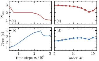
Figure 1: Analysis of the ITO propagator’s numerical efficiency: Mean number of iterations per time step $N_{\mathrm{iter}}$ and elapsed CPU time $T_{\text{CPU}}$ vs. the total number of time steps $n_{t}$ (a, b) and the expansion order $M$ (c, d). The system parameters (cf. Eqs. (11)-(12)) are $m=\omega=1$, $\mathcal{E}_{0}=10^{-3}$, $\omega_{L}=5$, $T=100$ with $M=8$ (a, b) and $n_{t}=900$ (c, d); the desired accuracy is $\epsilon=10^{-12}$.

We analyze the numerical effort as a function of both parameters in Fig. 1. The upper panel shows the number of iterations $N_{\mathrm{iter}}$ required to reach an accuracy of $10^{-12}$ as a function of the number of time steps $n_{t}$ (which is inversely proportional to $\delta t$ for fixed $T$) and the order $M$ of the inhomogeneity. The lower panel displays additionally the elapsed CPU time $T_{\mathrm{CPU}}$ for that computation . A direct correlation between the required number of iterations and the CPU time is observed: In Fig. 1(b), two sharp bends occur – the first one at the point where $2$ iterations begin to suffice to reach convergence, at roughly $n_{t}=700$; prior to that, on average, $2$ to $3$ iterations were required. Between $n_{t}=700$ and $1900$, there is a plateau in the required number of iterations, since the increase of $n_{t}$, i.e. decrease of $\delta t$, did not suffice to reach convergence within less iterations, although the accuracy (per iteration) was increased. During this plateau, the increased number of time steps thus only leads to a larger numerical effort, as can be seen in the CPU time. The second bend is the larger one, at $n_{t}=1900$, where the propagator first was able to reach convergence within one single iteration, for some of the time steps, leading to $N_{\mathrm{iter}}$ between $1$ and $2$. Further decrease of this quantity due to decrease of $\delta t$ rapidly improved the CPU time, until – again – a plateau is reached at $N_{\mathrm{iter}}=1$. At this point, a further decrease of $\delta t$ is not reasonable, since it can only increase the numerical effort without any gain, because less than one iteration is of course not possible.

A similar relation between $T_{\text{CPU}}$ and $N_{\mathrm{iter}}$ can be observed in Fig. 1(c, d). For constant $\delta t$, an increase in $M$ leads to higher CPU times up to the point where the number of iterations is noticeably reduced below $3$. The effort decreases then, until $N_{\mathrm{iter}}=2$ is reached. Interestingly, $N_{\mathrm{iter}}$ increases again when further increasing $M$. This is counter-intuitive, since a higher order should decrease the number of iterations. However, for too high orders $M$ numerical instabilities occur in the interpolation of the inhomogeneity in orthogonal polynomials. In fact, for $M>16$ the procedure does not converge at all. Failure to reach convergence happens, of course, also for too small $M$ since then the inhomogeneity is not represented accurately enough. Between these two limits, the curve in Fig. 1(d) shows only a weak dependence on the order $M$, indicating a surprisingly low impact of this parameter on the efficiency. This can be explained as follows: Larger $M$ increases the cost of each iteration while, at the same time, decreasing the average number of iterations, $N_{\mathrm{iter}}$. The two effects approximately cancel out in the end, leading to an almost constant dependence of $T_{\text{CPU}}$ on $M$. In conclusion, $M$ should be chosen carefully in accordance with the time step size, with $M=8$ representing a good starting point.

We now address the question of how iterative time ordering compares to the PWC approximation. For the latter, we employ the Chebyshev propagator Tal-Ezer and Kosloff (1984) where, for a given $\delta t$, the number of coefficients $n_{\text{c}}$ required in order to reach machine precision are calculated. Hence, the time-independent problem is solved with maximal precision and the only inaccuracy is due to the PWC approximation. In other words, there is only one free parameter, which also determines precision – $\delta t$ or the number of time steps $n_{t}$.

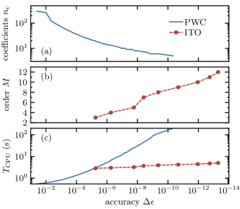
Figure 2: Comparison of iterative time ordering and the PWC approximation using the Chebyshev propagator: (a) Number of Chebyshev coefficients $n_{\text{c}}$, (b) ITO expansion order $M$, and (c) elapsed CPU time $T_{\text{CPU}}$ vs. desired accuracy $\Delta\epsilon$. The system parameters are as in Fig. 1, except for $\omega_{L}=1.001$, corresponding to near-resonant driving, and $T=1000$.

Figure 2 compares the CPU time required to reach a certain accuracy for the two propagation approaches. The accuracy corresponds to the maximal deviation of the numerical solutions from the analytical one. For the Chebyshev propagator and the PWC approach, we continuously increased $n_{t}$, respectively decreased $\delta t$, in order to continuously improve the quality of the PWC approximation. Figure 2(a) shows the number of required Chebyshev coefficients $n_{\text{c}}$ within each time step $\delta t$. We observe a strong decrease of $n_{\text{c}}$ (as $\delta t$ decreases from left to right) from about $300$ to $5$ in the end. For the ITO propagator, the number of time steps was set constant to $n_{t}=4000$, and only the order $M$ was varied, between $3$ and $12$, as shown in Fig. 2(b). This leads to accuracies between $6\cdot 10^{-5}$ and $5\cdot 10^{-14}$. Larger inaccuracies could not be realized with the ITO propagator. The lower limit is close to, but above machine precision and is due to accumulation of errors. Accumulation of errors is of course also – and especially – a problem for the PWC approach, where up to $10$ million time steps were required to achieve the higher accuracies. The smallest error that can realized in the PWC approach amounts to about $\Delta\epsilon\sim 10^{-11}$; further decreasing $\delta t$ does not push the error to below this value. In contrast, the ITO propagator avoids the accumulation of errors and allows for realizing errors much closer to machine precision over the complete propagation time interval.

The CPU time increases almost linearly with the accuracy for the PWC propagations in the double-logarithmic plot as well, corresponding to an approximately cubic dependence. For the ITO propagator, the increase in CPU time with the accuracy is significantly weaker. The required CPU time varied from $2.84\text{\,}\mathrm{s}$ to $5.01\text{\,}\mathrm{s}$ for ITO and from $0.53\text{\,}\mathrm{s}$ to $199\text{\,}\mathrm{s}$ for the PWC approximation. An interesting point is at about $\Delta\epsilon=10^{-5}$, where the two curves nearly intersect. If an accuracy higher than this value is required, the ITO propagator easily outperforms the PWC approach; the higher the accuracy, the more obvious this is. For lower accuracies, however, the PWC approach remains the best choice, being both stable and very fast. It should be noted that this threshold of $\Delta\epsilon$ cannot be generalized, since it depends on the strength of the time dependence of the problem at hand. While no rigorous measure to quantify the strength of the time dependence has, to the best of our knowledge, so far been brought forward, it is increased (decreased) in our example in Fig. 2 by increasing (decreasing) $\omega_{L}$ or $\mathcal{E}_{0}$ in Eq. (12). As a consequence, the threshold of $\Delta\epsilon$ decreases (increases) accordingly.

III.2 Benchmarking Krotov’s Method for Quantum Optimal Control with Iterative Time Ordering

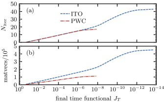
Figure 3: Comparison of the ITO (dashed) and PWC (dash-dotted) propagators when used in Krotov’s method: (a) Number of iterations $N_{\text{iter}}$ and (b) number of matrix-vector operations required to reach a certain value of the functional $J_{T}$. The considered system is the HO as in Eq. (14) where the frequency is controlled ($T=2$, $\delta t=0.01$, $M=5$).

We now determine the numerical effort required to reach a certain quality of the optimization result. The system to be controlled is once again the HO, this time described by a slightly different Hamiltonian,

$$\boldsymbol{\mathsf{\hat{H}}}_{\text{freq}}(t)=\frac{\boldsymbol{\mathsf{\hat{p}}}^{2}}{2}+\frac{1}{2}\boldsymbol{\mathsf{\hat{x}}}^{2}\mathcal{E}(t),$$ (14)

i.e., we set $\omega=m=1$. Equation (14) represents an example which is controllable, in contrast to Eq. (11), which is uncontrollable due to the equidistant energy levels. The control function $\mathcal{E}(t)$ effectively represents the frequency (or rather its square) of the harmonic potential which alters the system’s eigenstates. We begin in the ground state $\ket{\psi_{0}}$ of the HO for $\omega=1$ and seek to transfer it into the ground state of a HO with $\omega=1/2$, by varying the harmonic potential’s frequency via $\mathcal{E}(t)$. The effort is measured in terms of number of iterations $N_{\text{iter}}$ and performed matrix-vector operations to reach a given fidelity or final time functional value,

$$J_{T}[\psi(T)]=1-|\braket{\psi(T)}{\psi_{\text{target}}}|^{2}.$$ (15)

$J_{T}$ measures the difference between the final state $\ket{\psi(T)}$ and the target state $\ket{\psi_{\text{target}}}$.

The results of the benchmark are shown in Fig. 3. The improvement per control iteration is very similar for both methods up until around $J_{T}\approx 10^{-6}$ with ITO incurring a higher numerical cost. When continuing the optimization towards even more accurate controls, the PWC method could decrease $J_{T}$ further to around $10^{-8}$, whereas ITO reached a value of nearly $10^{-14}$. Again, being a more costly method than PWC, ITO requires a larger number of operations for an equal amount of iterations, cf. Fig. 3(b). In contrast to the PWC approximation with which Krotov’s method breaks down at around $J_{T}=10^{-8}$ since the errors in the time propagation do not allow for further improvements of the control, Krotov’s method with the ITO propagator can reach the control target with essentially arbitrary (i.e., close to machine precision) accuracy.

The solutions are found to be identical up to slight variations which are due to the higher accuracy of the ITO propagator and account for the difference in the fidelities beyond $J_{T}\approx 10^{-6}$. We conclude that, for the HO, the combination of Krotov’s method with iterative time ordering allows for more accurate control solutions. However, this will turn out to be not a general feature, as we show below. The higher accuracy comes at the price of a larger numerical effort which increases linearly for exponentially smaller errors.

IV Pythagorean Control of a Superconducting Qudit under Strong Driving

A more realistic application for the previously introduced propagator occurs in the dynamics of superconducting qubits, where driving fields are often rapidly oscillating in time. Here, we consider a superconducting qubit under Pythagorean control Suchowski et al. (2011); Svetitski et al. (2014).

IV.1 Model

Quantized superconducting circuits can encode information in their lowest few energy eigenstates, since the dynamics can be confined experimentally to these relevant levels Gambetta et al. (2017). For the lowest eigenstates, the ‘qubit’ can be modeled by an anharmonic ladder, not necessarily ending after two (qubit) levels. Therefore, we use the term qudit in the following. The Hamiltonian for a driven $N$-level qudit reads

$$\boldsymbol{\mathsf{\hat{H}}}(t)=\boldsymbol{\mathsf{\hat{H}}}_{0}+\boldsymbol{\mathsf{\hat{H}}}_{1}(t)$$ (16)

with drift Hamiltonian ($\hbar=1$)

$$\boldsymbol{\mathsf{\hat{H}}}_{0}=\sum_{n=0}^{N-1}\epsilon_{n}\Ket{n}\Bra{n}, \epsilon_{n}=n\omega_{0}-\frac{\beta}{2}n(n-1),$$

where $\epsilon_{n}$ is the eigenenergy for eigenstate $\Ket{n}$ of $\boldsymbol{\mathsf{\hat{H}}}_{0}$. The parameter $\omega_{0}$ defines the base energy difference between adjacent levels of the qudit and $\beta$ determines its anharmonicity. The control Hamiltonian is given by

$$\boldsymbol{\mathsf{\hat{H}}}_{1}(t)=\sum_{n=0}^{N-2}\sqrt{n+1}\Big{[}\Ket{n}\Bra{n+1}+\text{H.c.}\Big{]}\mathcal{E}(t),$$

where $\mathcal{E}(t)$ is the external control field and H.c. denotes the Hermitian conjugate.

As experimentally demonstrated in Ref. Svetitski et al. (2014), population inversion between non-adjacent levels of the four-level system can be realized using so called Pythagorean couplings Suchowski et al. (2011). The corresponding external field is given by Svetitski et al. (2014)

$$\mathcal{E}(t)=\frac{V_{01}}{\sqrt{1}}\cos\left(\omega_{01}t\right)+\frac{V_{12}}{\sqrt{2}}\cos\left(\omega_{12}t\right)+\frac{V_{23}}{\sqrt{3}}\cos\left(\omega_{23}t\right),$$ (17)

with $\omega_{ij}=\epsilon_{j}-\epsilon_{i}$ and $V_{ij}$ the driving strength of transition $\omega_{ij}$. Transforming Eq. (16) into the interaction picture yields (see Appendix B for details)

$$\boldsymbol{\mathsf{\hat{H}}}_{\text{int}}(t) =\frac{1}{2}\begin{pmatrix}0&V_{01}&0&0&0&\dots&0\\ V_{01}&0&V_{12}&0&0&\dots&0\\ 0&V_{12}&0&V_{23}&0&\dots&0\\ 0&0&V_{23}&0&0&\dots&0\\ 0&0&0&0&0&\dots&0\\ \vdots&\vdots&\vdots&\vdots&\vdots&\ddots&0\\ 0&0&0&0&0&\dots&0\\ \end{pmatrix}+\boldsymbol{\mathsf{\hat{H}}}_{\text{rot}}(t)$$

$$\equiv\boldsymbol{\mathsf{\hat{H}}}_{\text{inf}}+\boldsymbol{\mathsf{\hat{H}}}_{\text{rot}}(t).$$ (18)

The first, time-independent term $\boldsymbol{\mathsf{\hat{H}}}_{\text{inf}}$ matches exactly the requirements for Pythagorean control Suchowski et al. (2011), while the second, time-dependent term $\boldsymbol{\mathsf{\hat{H}}}_{\text{rot}}(t)$ contains co- and counter-rotating terms due to the rotating frame, cf. Appendix B. We neglect this term for a moment and assume Hamiltonian (IV.1) to be entirely given by $\boldsymbol{\mathsf{\hat{H}}}_{\text{inf}}$. In this case, the control scheme has been derived analytically Suchowski et al. (2011). In order to achieve population inversion between $\Ket{0}$ and $\Ket{2}$ (which we will consider in the following), the driving strengths $V_{ij}$ must be scaled by a primitive Pythagorean triple Suchowski et al. (2011),

$$\left(V_{01},V_{12},V_{23}\right)=\Omega_{\text{rabi}}\left(\frac{p^{2}+q^{2}}{2},pq,\frac{p^{2}-q^{2}}{2}\right),$$ (19)

with $p,q$ odd integers. For practical purposes, since the total magnitude of all $V_{ij}$ can be scaled by an experimentally accessible parameter (the Rabi frequency $\Omega_{\text{rabi}}$), we allow $p,q$ to take non-integer values.

Unfortunately, the additional term $\boldsymbol{\mathsf{\hat{H}}}_{\text{rot}}(t)$ in Eq. (IV.1) vanishes only in the unphysical limit of infinite anharmonicity $\beta$. We will analyze deviations below. To account for dissipative effects due to the interaction of the superconducting circuit with its environment, we employ a Lindblad master equation Breuer and Petruccione (2002)

$$\textup{i}\frac{\partial}{\partial t}\boldsymbol{\mathsf{\hat{\rho}}}(t) =\big{[}\boldsymbol{\mathsf{\hat{H}}}(t),\boldsymbol{\mathsf{\hat{\rho}}}(t)\big{]}+\boldsymbol{\mathsf{\mathcal{L}}}_{D}\left[\boldsymbol{\mathsf{\hat{\rho}}}(t)\right],$$

$$\boldsymbol{\mathsf{\mathcal{L}}}_{D}\left[\boldsymbol{\mathsf{\hat{\rho}}}(t)\right] =\textup{i}\sum_{k=1}^{2}\Big{(}\boldsymbol{\mathsf{\hat{L}}}_{k}\boldsymbol{\mathsf{\hat{\rho}}}(t)\boldsymbol{\mathsf{\hat{L}}}_{k}^{\dagger}-\frac{1}{2}\big{\{}\boldsymbol{\mathsf{\hat{L}}}_{k}^{\dagger}\boldsymbol{\mathsf{\hat{L}}}_{k},\boldsymbol{\mathsf{\hat{\rho}}}(t)\big{\}}\Big{)},$$

with Lindblad operators Reich et al. (2015)

$$\boldsymbol{\mathsf{\hat{L}}}_{1}=\sum_{n=0}^{N-2}\sqrt{\frac{n+1}{T_{1}}}\Ket{n}\Bra{n+1}, \boldsymbol{\mathsf{\hat{L}}}_{2}=\sum_{n=1}^{N-1}\sqrt{\frac{2n^{2}}{T_{2}^{*}}}\Ket{n}\Bra{n},$$

where $T_{1}$ is the population relaxation time and $T_{2}^{*}$ the pure dephasing time. The parameters of Tab. 1 are used in the following and the qudit ladder is truncated at $N=10$ levels, which was observed to suffice.

Table 1: The parameters for the Pythagorean controlled qudit, taken from Ref. Svetitski et al. (2014).

qudit frequency	$\omega_{0}/2\pi$	$6.73$ GHz
anharmonicity	$\beta/2\pi$	$0.12$ GHz
relaxation time	$T_{1}$	$230$ ns
dephasing time	$T_{2}$	$120$ ns
Rabi freqeuncy	$\Omega_{\text{rabi}}/2\pi$	$47.6$ MHz
field parameters	$p,q$	$0.86$

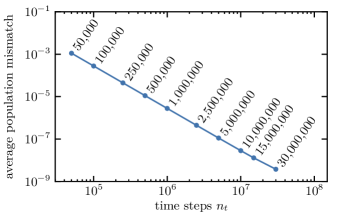
Figure 4: Average population mismatch when comparing propagations using the PWC method against a single propagation using ITO. The total propagation time is $T=150$ ns. Shown is the time-averaged maximal population mismatch, cf. Eq. (20). All simulations using the PWC propagator are compared against the same ITO propagation with $n_{t}=50{,}000$ constant time steps and $M=12$.

IV.2 Numerical Considerations for the ITO Propagator

Figure 4 proves that the ITO propagator also works for more complex systems than the HO; here for the qudit under Pythagorean control. The respective population dynamics (obtained with ITO) is depicted in Fig. 5. Since an analytical solution for the dynamics is not available in this case, we compare propagations using a PWC propagator (with an increasing number of time steps) to a single propagation using ITO. Here, we assume that any PWC propagator converges to an accurate time-ordered solution provided the time discretization is sufficiently fine. We quantify the mismatch between both simulations by taking the time-average of the function

$$P_{\text{mis}}(t)=\max_{n=0,\dots,N-1}\left|P_{n}^{\text{PWC}}(t)-P_{n}^{\text{ITO}}(t)\right|$$ (20)

with $P_{n}^{\text{PWC}}(t)$, $P_{n}^{\text{ITO}}(t)$ the populations in the $n$th level obtained with PWC or ITO propagation, respectively. As can be seen in Fig. 4, the mismatch of the population dynamics between PWC and ITO propagation decreases linearly with increasing number of PWC time steps $n_{t}$ in a double logarithmic plot. Since we assume increasing accuracy of the PWC propagation for increasing $n_{t}$, Fig. 4 clearly confirms that ITO holds its precision promise. Hence, in the following, we will assume that any propagation using ITO is accurate to at least $\mathcal{O}\left(10^{-9}\right)$.

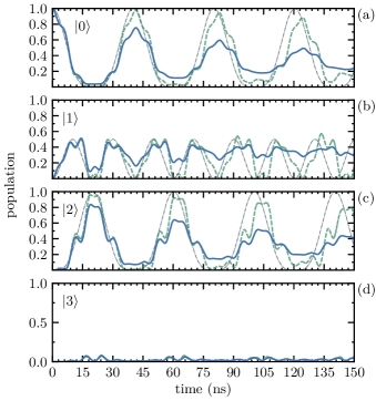
Figure 5: Population dynamics in the qudit subspace $\left\{\Ket{0},\Ket{1},\Ket{2},\Ket{3}\right\}$. The dash-dotted lines represent the ideal, non-dissipative case using only $\boldsymbol{\mathsf{\hat{H}}}_{\text{inf}}$, cf. Eq. (IV.1). The dashed (solid) lines show the non-dissipative (dissipative) population dynamics under Hamiltonian (16). The dissipative dynamics corresponds to the convergence analysis in Fig. 4.

The results of Fig. 4 already indicate the strong time-dependence of Hamiltonian (16). Commonly, the time-dependence of Hamiltonians can be reduced drastically by applying a rotating wave approximation (RWA). This has exemplarily been done for the interaction Hamiltonian (IV.1), cf. Eq. (31). Whether an RWA is a reasonable approximation depends, in general, on the actual system and problem, as well as the desired accuracy. However, ITO provides an excellent method for examining the quality of any RWA, since inaccuracies originating from numerical propagation are drastically diminished. When repeating the dissipation-free propagations of Fig. 5 (dashed lines) with the RWA-Hamiltonian (31), the average inaccuracy of the population dynamics becomes $\bar{P}_{\text{mis}}=1.3\cdot 10^{-3}$. The RWA thus turns out to be a poor approximation. Comparing the solid and dash-dotted lines in Fig. 5 reveals moreover that, in addition to the anharmonicity, also dissipation results in deviations from the ideal dynamics and hampers perfect population inversion. Experimentally, Ref. Svetitski et al. (2014) observed even more drastic discrepancies to Pythagorean control for high intensity. We therefore analyze the dynamics under such strong driving below.

IV.3 Dynamics under Strong Driving

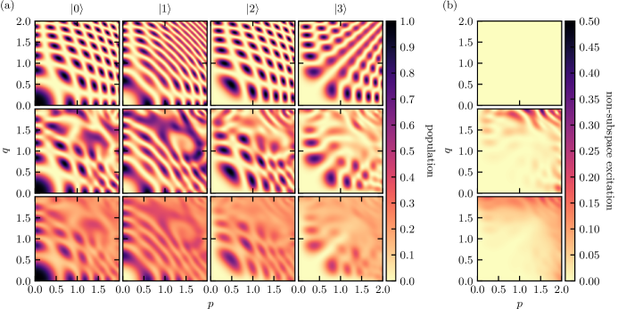
Figure 6: Final populations after applying the field (17) for $T=60$ ns. The upper row corresponds to the ideal, non-dissipative case of Eq. (IV.1) with only $\boldsymbol{\mathsf{\hat{H}}}_{\text{inf}}$. The middle (lower) row shows the propagation results with Hamiltonian (16) neglecting (including) dissipation. All simulations are performed using the ITO propagator. Part (a) shows the final population in states $\Ket{0},\Ket{1},\Ket{2},\Ket{3}$ as indicated on top of the four columns, part (b) the final population outside of the subspace $\left\{\Ket{0},\Ket{1},\Ket{2},\Ket{3}\right\}$.

Figure 6(a) shows the final population in the four states $\Ket{0}$, $\Ket{1}$, $\Ket{2}$, $\Ket{3}$ after a fixed propagation time of $T=60$ ns, obtained with fields of various intensities. Since the field is entirely determined by $p$ and $q$, cf. Eq. (19), the field intensity increases from the lower left to the upper right part within each panel. For the ideal, non-dissipative case, depicted in the upper row of Fig. 6(a), a regular pattern can be observed. In comparison, the middle row shows the results obtained with Hamiltonian (16). To emphasize the differences, dissipation has been neglected for the moment. We can clearly identify two different regions within each map. On the one hand, for weak field intensities, the ideal pattern is reproduced fairly well when taking the finite anharmonicity into account. On the other hand, for strong field intensities, the ordered structure visible in the upper row vanishes completely. When including dissipation, all maps become blurred (lower row), since the dissipation spreads the population across all levels. Nevertheless, the discrepancy between weak and strong field intensities appears with and without dissipation, i.e., the underlying effect is not related to dissipation. The solution to the puzzle can partly be found in Fig. 6(b), where the final population outside of the subspace $L=\text{span}\left\{\Ket{0},\Ket{1},\Ket{2},\Ket{3}\right\}$ is shown. In the ideal case (upper row), no population can leave $L$, since Hamiltonian $\boldsymbol{\mathsf{\hat{H}}}_{\text{inf}}$ in Eq. (IV.1) contains no coupling elements to any states $\Ket{n}$ with $n>3$. In contrast, $\boldsymbol{\mathsf{\hat{H}}}_{\text{rot}}(t)$, respectively Hamiltonian (16), does indeed contain such couplings. As visible in the middle and lower panels of Fig. 6(b), the population leakage out of subspace $L$ is rather small for weak fields but increases rapidly for strong fields. Moreover, in addition to pure loss of population from subspace $L$ at final time, the operator $\boldsymbol{\mathsf{\hat{H}}}_{\text{rot}}(t)$ will also increasingly influence the dynamics at intermediate times. In order to examine the impact of the operator, while neglecting, at the same time, loss of population from $L$, we truncate the qudit ladder at $N=4$. Note that this is definitively a bad approximation, since Fig. 6(b) has already shown the levels $\Ket{n}$ with $n>3$ to contribute significantly to the dynamics. Nevertheless, repeating the simulation of the middle row of Fig. 6 with $N=4$ (data not shown) yields a similar match for weak field intensities, or mismatch for strong field intensities, respectively, compared to the ordered structure of the ideal case. This shows that even without loss of population from the subspace $L$, the operator $\boldsymbol{\mathsf{\hat{H}}}_{\text{rot}}(t)$ compromises the ideal population inversion of Pythagorean control.

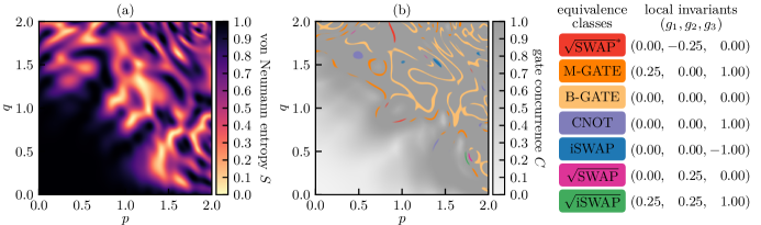
Figure 7: (a) shows the von Neumann entropy $S$ for the final states of Fig 6 (middle row). (b) shows the gate concurrence (gray shading in the background) for the implemented quantum gate. The colored areas indicate where the implemented gates are close to the respective local equivalence classes listed on the right.

Interestingly, the deviation from the ideal population inversion in Pythagorean control, caused by intense driving fields, gives rise to much richer dynamics in terms of implementable operations, i.e., quantum gates, on the subspace $\mathcal{L}$. As has be shown in Ref. Suchowski et al. (2011), $\boldsymbol{\mathsf{\hat{H}}}_{\text{inf}}$ allows only for quantum gates $\boldsymbol{\mathsf{\hat{O}}}\in\text{SO}(4)=\text{SU}(2)\otimes\text{SU}(2)$. One can interpret the four-level qudit as consisting of two virtual qubits by assigning one of the four two-qubit basis states to each of the qudit states $\Ket{0}$, $\Ket{1}$, $\Ket{2}$, $\Ket{3}$. In this picture, it is the ‘non-local’ operations that are missing in the ideal case, as they are element of $\text{SU}(4)\setminus\text{SO}(4)$. According to Ref. Svetitski et al. (2014), we choose the four Bell states $\{\Ket{\Phi^{\pm}},\Ket{\Psi^{\pm}}\}$ as two-qubit basis. Figure 7(a) shows the von Neumann entropy $S$ Bennett et al. (1996), as a measure of entanglement between the two virtual qubits, for the final states of Fig. 6(a) (middle row). As can be seen, weak fields are not able to change the amount of initial entanglement. This perfectly agrees with the observations in Fig. 6, since weak fields yield good agreement with the prediction of Pythagorean control. Thus, the implemented quantum gates are operations $\boldsymbol{\mathsf{\hat{O}}}\in\text{SO}(4)$, at least roughly so. For strong field intensities, the implemented quantum gates become entangling, as the change in $S$ indicates. The gate concurrence $C$ Kraus and Cirac (2001) can be used in order to quantify the entangling power of these quantum gates. It ranges from $C=0$ (non-entangling) to $C=1$ (maximally entangling) and is shown in Fig. 7(b) (gray background shading) for the final states of Fig. 7(a), respectively Fig. 6 (middle row). As can be seen, strong field intensities create maximally entangling gates for almost all combinations of $p$ and $q$.

We now analyze the implemented quantum gates. To this end, we perform a Cartan decomposition, which separates each gate into its local and non-local content Zhang et al. (2003). The non-local content unambiguously determines the entangling power of each gate. It is given by three real numbers, the local invariants $g_{1},g_{2},g_{3}$ Makhlin (2002). We call two gates $\boldsymbol{\mathsf{\hat{O}}}_{1},\boldsymbol{\mathsf{\hat{O}}}_{2}\in\text{SU}(4)$ locally equivalent and say they are in the same equivalence class $[\boldsymbol{\mathsf{\hat{O}}}_{1}]$, if they only differ by local operations $\boldsymbol{\mathsf{\hat{k}}}_{1},\boldsymbol{\mathsf{\hat{k}}}_{2}\in\text{SO}(4)$, i.e., $\boldsymbol{\mathsf{\hat{O}}}_{1}=\boldsymbol{\mathsf{\hat{k}}}_{1}\boldsymbol{\mathsf{\hat{O}}}_{2}\boldsymbol{\mathsf{\hat{k}}}_{2}$. It is straightforward to calculate the local invariants for all final gates of Fig. 7 and compare them against equivalence classes of common entangling two-qubit gates, cf. right column of Fig. 7. For strong field intensities, we find various regions, where the implemented gates are close to a specific equivalence class of entangling two-qubit gates. This shows, that depending on the field parameters $p,q$ for Pythagorean control, a large set of entangling two-qubit gates can be realized. Note that the check for closeness to an equivalence class is rather loose with $\left|\vec{g}-\vec{g}_{\text{ec}}\right|\leq 0.1$, $\vec{g}=\left(g_{1},g_{2},g_{3}\right)$ and $\vec{g}_{\text{ec}}$ corresponding to one of the triples shown on the right side of Fig. 7. Moreover, to counter the loss of population from the subspace $L$, which makes the actually implemented quantum gates non-unitary within $L$, a singular value decomposition has been applied in order to get the closest approximate unitary operation on $\mathcal{L}$. Therefore, the characterized gates are not accurate in terms of necessary gate fidelity for quantum computing Steane (2003). Nevertheless, they are still a hint towards the qudit’s natural evolution and, in particular, they emphasize the large amount of gates, which are accessible by varying $p,q$. Since gate generation in Fig. 7 is limited to the analytical pulse (17), it is natural to ask whether the gate fidelities can be improved when optimizing the pulse.

IV.4 Pythagorean Control using Krotov’s Method with ITO

We first check how Krotov’s method with ITO, as described in subsection II.2, performs for the qudit under Pythagorean control. We consider two control problems. First, in order to compare with Sec. III.2, the control problem is a state-to-state transition. Specifically, we seek to achieve population inversion from $\Ket{0}$ to $\Ket{2}$ where it would not occur naturally. The target functional is again given by Eq. (15). Second, in order to obtain a deeper understanding of Fig. 7, the control problem consists in implementing a predefined two-qubit gate $\boldsymbol{\mathsf{\hat{O}}}$ at final time $T$. To this end, the figure of merit $J_{T}$ in the optimization functional (9) is taken to be Palao and Kosloff (2003)

$$J_{T}[\{\Psi_{n}(T)\}]=1-\frac{1}{4}\mathfrak{Re}\bigg{\{}\sum_{n=0}^{3}\Braket{n}{\boldsymbol{\mathsf{\hat{O}}}^{\dagger}}{\Psi_{n}(T)}\bigg{\}}\,.$$ (21)

The set $\{\ket{\Psi_{n}(t)}\}$ corresponds to the forward propagated initial states $\{\Ket{n}\}$, given by the states from the subspace $L=\text{span}\{\Ket{0},\Ket{1},\Ket{2},\Ket{3}\}$. This control problem is significantly more challenging than a state-to-state optimization. In terms of control complexity, it is equivalent to optimizing simultaneously four state-to-state optimizations, one for each state in the logical basis Tesch and de Vivie-Riedle (2002); Palao and Kosloff (2002).

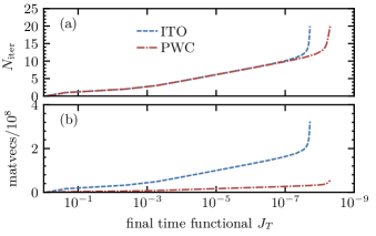
Figure 8: The same comparison as in Fig. 3, but for the qudit under Pythagorean control with the goal of realizing population inversion from $\Ket{0}$ to $\Ket{2}$ that does not occur naturally ($p=q=0.5$ for the guess pulse, $T=150\,$ns, $\delta t=0.001\,$ns, $M=6$).

For the first control problem, Fig. 8 compares the performance of Krotov’s method when used with the Chebychev propagator in the PWC approximation and the ITO propagator, respectively. While the optimization requires the same amount of iterations to reach a certain quality of the control, using ITO comes with a larger numerical effort, as evidenced by the larger number of matrix vector operations in Fig. 8(b). These findings are similar as those for controlling the harmonic oscillator, reported in Fig. 3. In contrast to Fig. 3, however, optimization based on the ITO propagator cannot reach smaller values of $J_{T}$, i.e., more accurate controls. The saturation of the optimization for the ITO propagator that is seen in the blue dashed line becoming vertical, is most likely due to a rather high sensitivity of the algorithm on the ITO parameters $\delta t$ and $M$ as well as the Krotov update parameter $\lambda_{a}$, cf. Eq. (10a).

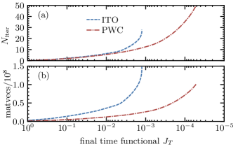
Figure 9: The same comparison as in Fig. 3, but for the qudit under Pythagorean control and the CNOT gate as target operation $\boldsymbol{\mathsf{\hat{O}}}$, cf. Eq. (21) ($T=150\,$ns, $\delta t=0.003\,$ns, $M=8$).

For the second control example, optimization of a CNOT gate, the difficulties of Krotov’s method when using ITO propagation become even more pronounced, see Fig. 9. The fact, that the control problem itself is more challenging is evidenced in Fig. 9 by the achievable values of $J_{T}$, respectively the error, being much larger than in Fig. 8 for both methods. But the multi-target optimization involves yet another difficulty for the ITO propagator. The optimal choice of its parameters $\delta t$ and $M$ must now be balanced between four different propagations. Given the sensitivity of the method on these parameters, convergence becomes more difficult to achieve. It turns out that smaller values of $M$, around $M=5$ or 6, should be used for stable optimizations, in comparison to a stable, stand-alone propagation. The optimal value of $M$ depends of course on the time step $\delta t$, which has to be chosen accordingly (small) such that a small $M$ suffices. For maximal efficiency, a tradeoff has to be found where the values are small enough for sufficient stability but not so small as to be numerically too costly. But even in this case, optimization with the ITO propagator requires significantly more computational resources than with the PWC approximation, cf. Fig. 9.

IV.5 Controllability and Quantum Speed Limit

Apart from the problem of finding optimized fields that implement a desired dynamics, such as a specific quantum gate, OCT can be used to answer, at least approximately, the more fundamental question of controllability Jurdjevic and Sussmann (1972); Huang et al. (1983): When starting from a given state $\ket{\Psi^{\text{init}}}$, which set of states $\left\{\ket{\Psi}\right\}$ is generally accessible under the set of all possible controls? The notion of quantum speed limits (QSLs) naturally arises in this context Lloyd (2000); Levitin and Toffoli (2009): Provided that a specific state $\ket{\Psi^{\text{targ}}}$ is accessible by the system’s dynamics starting in $\ket{\Psi^{\text{init}}}$, what is the minimal time for this transition? The notion of quantum speed limit is particularly important with respect to unwanted interaction with the environment since it tells us whether it is possible to ‘beat’ decoherence using optimized controls Koch (2016).

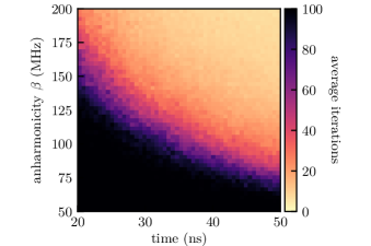
Figure 10: Optimization results for random unitary operations with the optimizations performed for various final times $T$ and varying qudit anharmonicities $\beta$. The guess fields, cf. Eq. (17), with $p=q=2$, were shaped on input by a linear rise and fall time of $10\%$ of $T$. Optimizations were repeated $30$ times and stopped at $100$ iterations if $J_{T}<10^{-3}$, cf. Eq. (21), could not be achieved until then.

Figure 10 provides information about the qudit’s controllability in two ways. On one hand, it numerally shows full qudit controllability. On the other hand, it allows to extract the QSL for the implementation of any two-qubit gate. The figure shows optimization results (using Krotov’s method in combination with a PWC propagator) for a variation of the final time $T$ and the anharmonicity $\beta$ of the qudit. Note that in order to focus on the influence of both parameters, dissipative effects have been neglected. For each combination of $T$ and $\beta$, $30$ random unitary gates $\boldsymbol{\mathsf{\hat{O}}}$ have been chosen Mezzadri (2007) as optimization target and the average required number of iterations in order to reach $J_{T}<10^{-3}$ is shown. The obtained map can be clearly divided into two regions. In the lower left part of Fig. 10, the optimization algorithm was not able reach $J_{T}<10^{-3}$ within the allowed $100$ iterations. Most likely, it will neither be possible for a larger number of iterations. In contrast, in the upper right part, the optimization algorithm finds suitable fields within only a few iterations, yielding gates with sufficiently low errors. This is numerical evidence for full controllability as the target gates were chosen randomly. The edge between both regions can be identified as the QSL for these operations. It is not sharp, since a tradeoff between remaining gate error $J_{T}$ and total time $T$ must usually be taken into account. Nevertheless, it decreases for increasing qudit anharmonicity. For the parameters in Tab. 1, the QSL can be roughly identified as $T\approx 35\,\text{ns}$. In order to have faster gates, the anharmonicity $\beta$ must be increased. Hence, increasing $\beta$ would benefit the qudit, as it reduces the impact of dissipation by allowing for generally faster operations. Apart from gate optimization, an increased $\beta$ would furthermore benefit the intended population inversion of Pythagorean control, cf. subsection IV.3, since it would diminish the strong field deviations originating from the finite anharmonicity.

V Conclusions

In order to assess the impact of time ordering in quantum optimal control, we have combined Krotov’s method with a highly efficient propagation method that explicitly accounts for time ordering. We have tested the ensuing algorithm for the harmonic oscillator and applied it to a superconducting circuit. For the latter, we have also analyzed the population dynamics, starting from so-called Pythagorean control for population inversion between non-adjacent levels in a four-level system Suchowski et al. (2011). For strong driving, the dynamics of the superconducting qubit had been found experimentally to significantly deviate from what is expected for Pythagorean control Svetitski et al. (2014). We could explain this observation in terms of higher levels in the anharmonic ladder that get populated which is a direct consequence of the failure of the rotating wave approximation. Furthermore, we have analyzed the time evolutions that can be generated in the superconducting circuit by determining the type of ‘non-local’ operations that can be realized. This analysis suggested full controllability of the superconducting qubit, a fact that we have confirmed by optimizing for random unitaries and determining the quantum speed limit for each. The latter is essentially determined by the anharmonicity.

Surprisingly, in our examples for OCT we have found the effect of time ordering to be fairly small. Except for very small control errors, the control solutions found within the piecewise constant approximation do not differ too much from those obtained under explicit time ordering. For very high precision applications as required, for example, in quantum information science below the error correction threshold, time ordering will, however, eventually become an effect that needs to be accounted for. At this time, iterative time ordering Ndong et al. (2010); Tal-Ezer et al. (2012); Schaefer et al. (2017) provides the most efficient approach to address this issue.

Iterative time ordering rewrites the explicitly time-dependent part of the equation of motion as an inhomogeneity that needs to be determined self-consistently. When combining this propagator with Krotov’s method, it turned out to be crucial to jointly determine both the control and the state self-consistently to obtain a converging method. Still, the performance of the resulting algorithm is rather sensitive with respect to its main parameters – the expansion order of the inhomogeneity, the time step and the magnitude of the control update. Should the algorithm be useful for practical applications, these parameters need to be determined in a more automated way to avoid numerical instability. This will be the subject of future work.

Author Contribution Statement

DB and LM contributed equally to this work, both in implementing code, running simulations and writing and revising the manuscript. CPK conceived the work and contributed to writing and revising of the manuscript.

Appendix A Implementation of the ITO Propagator

Figure 11: The ITO propagator as pseudo code algorithm.

The pseudocode for the ITO propagator is shown in Fig. 11. Curved brackets indicate a loop over all elements of the set, where the indices $i,j,m,n$ range from 0 to $M-1$. For better readability, only the most important steps are included in Fig. 11. When implementing the code for the ITO algorithm, several aspects have to be taken into account.

(i) Transformation of the polynomial expansion of the inhomogeneity into the monomial basis: First, we expand Newton polynomials $R_{n}$ in the monomial basis,

$$R_{n}(t)=\sum_{m=0}^{n}q_{n,m}\frac{t^{m}}{m!}\,.$$ (22)

Making use of the recursive definition of the Newton polynomials and by equating coefficients, we obtain

$$q_{n+1,0} =-t_{n}q_{n,0}\,,$$ (23a)

$$q_{n+1,m} =mq_{n,m-1}-t_{n}q_{n,m}\,,$$ (23b)

$$q_{n+1,n+1} =\left(n+1\right)q_{n,n}\,,$$ (23c)

from which, with $q_{0,0}=1$, all transformation coefficients can be computed recursively. The inhomogeneity expanded in orthogonal Newton polynomials, with polynomial coefficients $a_{n}$, can then be transformed into the monomial basis,

$$s(t)\approx\sum_{m=0}^{M-1}s_{m}\frac{t^{m}}{m!}, s_{m}=\sum_{n=m}^{M-1}q_{n,m}a_{n}.$$

(ii) Normalization of the expansion domain: In the case of the Chebyshev polynomials as polynomial basis, this is essential, since they can only be used on the interval $[-1,+1]$. For the Newton polynomials, a normalization also becomes necessary when computing the coefficients by the divided difference scheme. Because of the recursive definition, including products of the differences between interpolating points in the denominator of the fraction, this might become unstable depending on how small or large these differences are. The optimal choice for stability is a domain of length $4$ which leads to a capacity $\rho$ of size $1$ Tal-Ezer (1991). This is desirable. The capacity $\rho=\prod_{i=1}^{N}|z_{i}-z_{\text{c}}|^{1/N}$, where $z_{\text{c}}$ is the center of the points $\{z_{i}\}$, is a measure for size and variance of the set $\{z_{i}\}$. To obtain it, one has to take the factor $4/\delta t$ into account for the computation of the Newton coefficients and later when using them in the transformation to monomial coefficients, see (i).

(iii) The product of the operator generating the dynamics and the time step, $G\delta t$: It is recommended that this product is carried out as it is, and that separating $G$ and $\delta t$ is avoided. As a matter of fact, the solution contains only terms with both the operator $G$ (or its eigenvalues) and the time step $\delta t$, neither of them individually. It might be the case that either the eigenvalues of $G$ are large or that $\delta t$ is small, and their joint evaluation avoids numerical instabilities.

(iv) Calculation of the function $f_{M}$: An especially crucial point is the computation of $f_{M}(G_{0},\{\tau_{j}\})v_{M}$, where instabilities occur if it is not computed thoroughly enough. Observing the definition of the function $f_{M}$, cf. Eq. (8a), we can see that the second term of the rhs is just a truncated exponential sum subtracted from the full exponential function. For small $zt$, the computation in this way might become unstable or inaccurate due to round-off errors. Instead, it is possible to directly calculate the expression in terms of an exponential series, starting at $M$. This decreases the round-off error by removing the subtraction.

(v) Error estimation for multiple sources of errors: The first – and usually largest – source of error occurs in the self-consistent loop to generate the solution, i.e., it is due to the fact that we have replaced the exact solution $u$ by the iterated one $u^{(k)}$, cf. Eq. (5). In order to determine how many iterations are needed, we use the common approach to compare the new solution $u^{(k)}$ to the one from the previous iteration $u^{(k-1)}$,

$$\epsilon_{\mathrm{iter}}^{(k)}\coloneqq\frac{\left\|u^{(k)}(t_{n+1})-u^{(k-1)}(t_{n+1})\right\|}{\left\|u^{(k)}(t_{n+1})\right\|}.$$

The second error originates from the approximation of the inhomogeneity $s(t)$ by a truncated polynomial expansion in time. This error can be estimated by Schaefer et al. (2017)

$$\epsilon_{M}\coloneqq\big{\|}\Delta s\big{\|}\delta t,$$ (24)

where $\|\Delta s\|$ represents the maximal interpolation error of the approximated inhomogeneity within the current time step. For the Newton interpolation on the Chebyshev nodes, cf. Eq. (7), it scales as $1/(2^{M-1}M!)$. Compared to $\epsilon_{\text{iter}}$, it has a smaller impact onto the total error due to the chosen splitting of the Hamiltonian, which we chose such that the inhomogeneity is small compared to the homogeneous part. The third and last source of error is the computation of $f_{M}(G_{0},\tau)v_{M}$, cf. Eq. (8a). Depending on $G$, the impact of this term might be very high in the computation. In general, if one or more of the errors are too high, it is recommended to either increase the order of the interpolating polynomial $M$ or decrease the size of the local interval, i.e., the time step $\delta t$.

Appendix B Derivation of the $N$-level Interaction Hamiltonian

The Hamiltonian (in its generalized $N$-level form) for the superconducting phase qudit is given by Eq. (16). The external control field $\mathcal{E}(t)$ is analytically given by Eq. (17). In the following, we transform states and operators into the interaction picture. For state $\Ket{\Psi(t)}$ in the Schrödinger picture, the transformation reads

$$\Ket{\Psi_{\text{int}}(t)}=\boldsymbol{\mathsf{\hat{O}}}(t)\Ket{\Psi(t)},\qquad\boldsymbol{\mathsf{\hat{O}}}(t)=\exp\left(\textup{i}\boldsymbol{\mathsf{\hat{H}}}_{0}t\right).$$ (25)

Plugging this into the Schrödinger equation yields

$$\textup{i}\frac{\partial}{\partial t}\Ket{\Psi_{\text{int}}(t)}=\boldsymbol{\mathsf{\hat{H}}}_{\text{int}}(t)\Ket{\Psi_{\text{int}}(t)}$$ (26)

with $\boldsymbol{\mathsf{\hat{H}}}_{\text{int}}(t)=\boldsymbol{\mathsf{\hat{O}}}(t)\boldsymbol{\mathsf{\hat{H}}}_{1}(t)\boldsymbol{\mathsf{\hat{O}}}^{\dagger}(t)$. Inserting two identity operators allows to write the interaction Hamiltonian as

$$\boldsymbol{\mathsf{\hat{H}}}_{\text{int}}(t)=\sum_{n,m=0}^{N-1}\boldsymbol{\mathsf{\hat{O}}}(t)\Ket{n}\Bra{n}\boldsymbol{\mathsf{\hat{H}}}_{1}(t)\Ket{m}\Bra{m}\boldsymbol{\mathsf{\hat{O}}}^{\dagger}(t).$$ (27)

Expanding the matrix element of $\boldsymbol{\mathsf{\hat{H}}}_{1}(t)$ gives

$$\boldsymbol{\mathsf{\hat{H}}}_{\text{int}}(t) =\sum_{n,m=0}^{N-1}\sqrt{n+1}\mathcal{E}(t)\delta_{m,n+1}e^{-\textup{i}\omega_{n,m}t}\Ket{n}\Bra{m}+\text{H.c.}$$ (28)

$$=\sum_{n=0}^{N-2}\sqrt{n+1}\mathcal{E}(t)e^{-\textup{i}\omega_{n,n+1}t}\Ket{n}\Bra{n+1}+\text{H.c.}$$

with $\omega_{n,n+1}=\epsilon_{n+1}-\epsilon_{n}$. Expanding the analytical field equation (17) in exponentials reads

$$\mathcal{E}(t) =\frac{1}{2}\left[\frac{V_{01}}{\sqrt{1}}\left(e^{\textup{i}\omega_{01}t}+e^{-\textup{i}\omega_{01}t}\right)+\frac{V_{12}}{\sqrt{2}}\left(e^{\textup{i}\omega_{12}t}+e^{-\textup{i}\omega_{12}t}\right)\right.$$ (29)

$$\qquad\left.+\frac{V_{23}}{\sqrt{3}}\left(e^{\textup{i}\omega_{23}t}+e^{-\textup{i}\omega_{23}t}\right)\right].$$

Plugging this into Eq. (28), we obtain the complete form of the interaction Hamiltonian as

$$\boldsymbol{\mathsf{\hat{H}}}_{\text{int}}(t)= \frac{1}{2}\left[\sum_{n=0}^{N-2}\sqrt{n+1}\Ket{n}\Bra{n+1}\times\right.$$ (30)

$$\hskip 5.69054pt\left.\left(\hphantom{+}\frac{V_{01}}{\sqrt{1}}\left(e^{\textup{i}\left(\omega_{01}-\omega_{n,n+1}\right)t}+e^{-\textup{i}\left(\omega_{01}+\omega_{n,n+1}\right)t}\right)\right.\right.$$

$$\hskip 11.38109pt\left.\left.+\frac{V_{12}}{\sqrt{2}}\left(e^{\textup{i}\left(\omega_{12}-\omega_{n,n+1}\right)t}+e^{-\textup{i}\left(\omega_{12}+\omega_{n,n+1}\right)t}\right)\right.\right.$$

$$\hskip 11.38109pt\left.\left.+\frac{V_{23}}{\sqrt{3}}\left(e^{\textup{i}\left(\omega_{23}-\omega_{n,n+1}\right)t}+e^{-\textup{i}\left(\omega_{23}+\omega_{n,n+1}\right)t}\right)\right)\vphantom{\sum_{n=0}^{N-2}}\right]$$

$$+\text{H.c.}$$

If we perform a rotating wave approximation, i.e. neglecting fast oscillating terms, the interaction Hamiltonian becomes

$$\boldsymbol{\mathsf{\hat{H}}}_{\text{int}}(t)= \frac{1}{2}\left[\sum_{n=0}^{N-2}\sqrt{n+1}\Ket{n}\Bra{n+1}\times\right.$$ (31)

$$\hskip 5.69054pt\left.\left(\hphantom{+}\frac{V_{01}}{\sqrt{1}}e^{\textup{i}\left(\omega_{01}-\omega_{n,n+1}\right)t}+\frac{V_{12}}{\sqrt{2}}e^{\textup{i}\left(\omega_{12}-\omega_{n,n+1}\right)t}\right.\right.$$

$$\hskip 11.38109pt\left.\left.+\frac{V_{23}}{\sqrt{3}}e^{\textup{i}\left(\omega_{23}-\omega_{n,n+1}\right)t}\right)\vphantom{\sum_{n=0}^{N-2}}\right]+\text{H.c.}$$

Eqs. (30) and (31) can be further divided into a time-independent and time-dependent part, such that the final form matches Eq. (IV.1).

References

- Glaser et al. (2015) S. J. Glaser, U. Boscain, T. Calarco, C. P. Koch, W. Köckenberger, R. Kosloff, I. Kuprov, B. Luy, S. Schirmer, T. Schulte-Herbrüggen, D. Sugny, and F. K. Wilhelm, Eur. Phys. J. D 69, 279 (2015).
- Werschnik and Gross (2007) J. Werschnik and E. K. U. Gross, J. Phys. B 40, R175 (2007).
- Khaneja et al. (2005) N. Khaneja, T. Reiss, C. Kehlet, T. Schulte-Herbrüggen, and S. J. Glaser, J. Magn. Reson. 172, 296 (2005).
- Castro et al. (2012) A. Castro, J. Werschnik, and E. K. U. Gross, Phys. Rev. Lett. 109, 153603 (2012).
- Hellgren et al. (2013) M. Hellgren, E. Räsänen, and E. K. U. Gross, Phys. Rev. A 88, 013414 (2013).
- Greenman et al. (2015) L. Greenman, C. P. Koch, and K. B. Whaley, Phys. Rev. A 92, 013407 (2015).
- Goetz et al. (2016) R. E. Goetz, A. Karamatskou, R. Santra, and C. P. Koch, Phys. Rev. A 93, 013413 (2016).
- Somlói et al. (1993) J. Somlói, V. A. Kazakovski, and D. J. Tannor, Chem. Phys. 172, 85 (1993).
- Goerz et al. (2011) M. H. Goerz, T. Calarco, and C. P. Koch, J. Phys. B 44, 154011 (2011).
- Watts et al. (2015) P. Watts, J. Vala, M. M. Müller, T. Calarco, K. B. Whaley, D. M. Reich, M. H. Goerz, and C. P. Koch, Phys. Rev. A 91, 062306 (2015).
- Goerz et al. (2015) M. H. Goerz, G. Gualdi, D. M. Reich, C. P. Koch, F. Motzoi, K. B. Whaley, J. Vala, M. M. Müller, S. Montangero, and T. Calarco, Phys. Rev. A 91, 062307 (2015).
- Ndong et al. (2010) M. Ndong, H. Tal-Ezer, R. Kosloff, and C. P. Koch, J. Chem. Phys. 132, 064105 (2010).
- Ndong et al. (2009) M. Ndong, H. Tal-Ezer, R. Kosloff, and C. P. Koch, J. Chem. Phys. 130, 124108 (2009).
- Tal-Ezer and Kosloff (1984) H. Tal-Ezer and R. Kosloff, J. Chem. Phys. 81, 3967 (1984).
- Tal-Ezer et al. (2012) H. Tal-Ezer, R. Kosloff, and I. Schaefer, J. Sci. Comput. 53, 211 (2012).
- Schaefer et al. (2017) I. Schaefer, H. Tal-Ezer, and R. Kosloff, J. Comput. Phys. 343, 368 (2017).
- Konnov and Krotov (1999) A. I. Konnov and V. F. Krotov, Autom. Rem. Contr. 60, 1427 (1999).
- Sklarz and Tannor (2002) S. E. Sklarz and D. J. Tannor, Phys. Rev. A 66, 053619 (2002).
- Palao and Kosloff (2003) J. P. Palao and R. Kosloff, Phys. Rev. A 68, 062308 (2003).
- Reich et al. (2012) D. M. Reich, M. Ndong, and C. P. Koch, J. Chem. Phys. 136, 104103 (2012).
- Kosloff (1994) R. Kosloff, Annu. Rev. Phys. Chem. 45, 145 (1994).
- Breuer and Petruccione (2002) H.-P. Breuer and F. Petruccione, The theory of open quantum systems, 1st ed. (Oxford University Press, 2002).
- Runge and Gross (1984) E. Runge and E. K. U. Gross, Phys. Rev. Lett. 52, 997 (1984).
- Marques and Gross (2004) M. A. L. Marques and E. K. U. Gross, Annu. Rev. Phys. Chem. 55, 427 (2004).
- Marques et al. (2012) M. A. L. Marques, N. T. Maitra, F. M. S. Nogueira, E. K. U. Gross, and A. Rubio, eds., Fundamentals of Time-Dependent Density Functional Theory, Lecture notes in physics, Vol. 837 (Springer, Berlin, Heidelberg, 2012).
- Hochbruck and Ostermann (2010) M. Hochbruck and A. Ostermann, Acta Numerica 19, 209–286 (2010).
- Salamin (1995) Y. I. Salamin, J. Phys. A 28, 1129 (1995).
- Note (1) The computer used for all computations is an Intel Core i7-5930 @ 3.50\tmspace+.1667emGHz system with 32\tmspace+.1667emGB RAM and a 64-bit Linux OS.
- Suchowski et al. (2011) H. Suchowski, Y. Silberberg, and D. B. Uskov, Phys. Rev. A 84, 013414 (2011).
- Svetitski et al. (2014) E. Svetitski, H. Suchowski, R. Resh, Y. Shalibo, J. M. Martinis, and N. Katz, Nat. Comm. 5, 5617 (2014).
- Gambetta et al. (2017) J. M. Gambetta, J. M. Chow, and M. Steffen, npj Quantum Inf. 3, 2 (2017).
- Reich et al. (2015) D. M. Reich, N. Katz, and C. P. Koch, Sci. Rep. 5, 12430 (2015).
- Bennett et al. (1996) C. H. Bennett, H. J. Bernstein, S. Popescu, and B. Schumacher, Phys. Rev. A 53, 2046 (1996).
- Kraus and Cirac (2001) B. Kraus and J. I. Cirac, Phys. Rev. A 63, 062309 (2001).
- Zhang et al. (2003) J. Zhang, J. Vala, S. Sastry, and K. B. Whaley, Phys. Rev. A 67, 042313 (2003).
- Makhlin (2002) Y. Makhlin, Quantum Inf. Process. 1, 243 (2002).
- Steane (2003) A. M. Steane, Phys. Rev. A 68, 042322 (2003).
- Tesch and de Vivie-Riedle (2002) C. Tesch and R. de Vivie-Riedle, Phys. Rev. Lett. 89, 157901 (2002).
- Palao and Kosloff (2002) J. P. Palao and R. Kosloff, Phys. Rev. Lett. 89, 188301 (2002).
- Jurdjevic and Sussmann (1972) V. Jurdjevic and H. J. Sussmann, J. Diff. Eqns. 12, 313 (1972).
- Huang et al. (1983) G. M. Huang, T. J. Tarn, and C. W. Clark, J. Math. Phys. 24, 2608 (1983).
- Lloyd (2000) S. Lloyd, Nature 406, 1047 (2000).
- Levitin and Toffoli (2009) L. B. Levitin and T. Toffoli, Phys. Rev. Lett. 103, 160502 (2009).
- Koch (2016) C. P. Koch, J. Phys.: Condens. Matter 28, 213001 (2016).
- Mezzadri (2007) F. Mezzadri, Notices of the AMS 54, 592 (2007).
- Tal-Ezer (1991) H. Tal-Ezer, SIAM J. Sci. Comput. 12, 648 (1991).