all
Automatic Symbolic Computation for Discontinuous Galerkin Finite Element Methods
Abstract
The implementation of discontinuous Galerkin finite element methods (DGFEMs) represents a very challenging computational task, particularly for systems of coupled nonlinear PDEs, including multiphysics problems, whose parameters may consist of power series or functionals of the solution variables. Thereby, the exploitation of symbolic algebra to express a given DGFEM approximation of a PDE problem within a high level language, whose syntax closely resembles the mathematical definition, is an invaluable tool. Indeed, this then facilitates the automatic assembly of the resulting system of (nonlinear) equations, as well as the computation of Fréchet derivative(s) of the DGFEM scheme, needed, for example, within a Newton-type solver. However, even exploiting symbolic algebra, the discretisation of coupled systems of PDEs can still be extremely verbose and hard to debug. Thereby, in this article we develop a further layer of abstraction by designing a class structure for the automatic computation of DGFEM formulations. This work has been implemented within the FEniCS package, based on exploiting the Unified Form Language. Numerical examples are presented which highlight the simplicity of implementation of DGFEMs for the numerical approximation of a range of PDE problems.
keywords:
Symbolic computation, finite element methods, discontinuous Galerkin methodsAMS:
65N301 Introduction
The finite element method (FEM) represents an indispensable computational tool for the accurate, efficient, and rigorous numerical approximation of continuum models arising within a wide range of scientific and engineering application areas. Key reasons for the success of FEMs include their applicability to very general classes of partial differential equations (PDEs), simple treatment of complicated computational geometries and enforcement of boundary conditions, ease of adaptivity including both local mesh subdivision (–refinement) and local polynomial enrichment (–refinement), and, from a mathematical point of view, the availability of tools for their rigorous error analysis. However, when compared with their finite difference counterparts, FEMs are typically regarded as being complicated to implement. Indeed, assembly of the underlying matrix stemming from the FEM discretisation of a given (linear, for example) PDE problem typically involves mapping each element present in the computational mesh, defined in the global coordinate system, to a given reference or canonical element, where both the local FEM basis and corresponding quadrature, needed to approximate the underlying integral, is defined. In this manner, local elemental stiffness matrices and load vectors may be computed; these entries are then inserted into the global matrix and right-hand side vector, respectively, according to the elementwise local-to-global degree of freedom mapping, subject to the enforcement of inter-element continuity constraints and the imposition of boundary conditions. This general assembly strategy is almost universally employed within both open source and commercial software, e.g., FreeFem++ [23], DUNE [8], deal.II [4] and OpenFOAM [40], to name just a few. Thereby, in principle, assuming that a user can define both the element stiffness matrix and load vector, then a numerical approximation may be readily determined. However, most open source software packages do not provide easy-to-use user interfaces; indeed, typically the user must first understand the low level language in which the code is written, e.g., C++, Fortran, etc, and develop an understanding of the underlying datastructures and function/subroutine calls defined within their chosen package in order to be able to develop code specific to their own application. This can, of course, be a rather time-consuming exercise, and often requires one to use multiple software libraries, for example, when certain features are not available within the chosen package which the user needs to utilise.
In the nonlinear setting, assuming a Newton-type iteration is exploited to solve the underlying system of nonlinear equations stemming from the given FEM employed, the general strategy of assembly of the resulting linearised equations is similar to the linear case; in this setting the load vector represents the residual of the numerical scheme. However, in this case, the Fréchet derivative of the FEM must now be computed; we point out that, in the context of the numerical detection of bifurcation points, the number of derivatives that must be computed just to form the so-called extended system needed to accurately compute the bifurcation point, even before a Newton iteration is implemented, is dependent on the codimension of the singularity being sought, cf. [10, 11]. In general, the evaluation and implementation of both the FEM residual and, moreover, the Fréchet derivative(s) of the scheme is a difficult and time consuming task, which is inevitably prone to human error. This is particularly the case when exploiting FEMs for the numerical approximation of systems of coupled nonlinear PDEs, including multiphysics problems, whose parameters may consist of power series or functionals of the solution variables, cf. [28].
Thus far, our discussion has primarily focussed on the application of conforming FEMs, whereby, excluding Neumann, or weakly imposed boundary conditions, only element contributions need to be evaluated. The exploitation of more general FEMs, and in particular discontinuous Galerkin FEMs (DGFEMs) requires the implementation of inter-element flux terms, which involves combinations of both inner– and outer–traces of the FEM solution, relative to a given orientation of the element face. In recent years, DGFEMs have become an increasingly popular class of FEMs, most notably due to their local conservation properties, inherent numerical stability for convection–dominated diffusion problems, limited interelement communication, which is restricted only to neighbouring elements, and has important advantages for the implementation of boundary conditions and the parallel efficiency of the method, and finally the ease in which so–called hanging nodes can be treated, and the efficient implementation of –adaptivity. Indeed, tremendous progress has been made on both the analytical and computational aspects of DGFEMs; for a review of some of the key developments in the subject, we refer to the recent monographs [13, 14, 24, 35]. For a historical review of DGFEMs, we refer to the articles [3, 12], and the references cited therein.
The addition of inter-element face terms within DGFEMs further complicates the implementation of such schemes within standard FEM packages. Assuming for a moment that the underlying PDE problem is linear, we note that for a given interior face, shared by two neighbouring elements, there are, in general, four local face matrices, which stem from the different combinations of traces of the FEM solution from the two elements whose boundaries form the current face. Once these local face–wise matrices have been assembled, they can then be inserted into the global FEM matrix in an analogous manner to the treatment of the element stiffness matrix. On boundary faces, contributions to the load vector must also be computed. Again, in the nonlinear setting, the task of computing both the residual vector and Fréchet derivative(s) of the DGFEM scheme is a very technical and time consuming task.
The purpose of this article is to discuss the use of symbolic algebra to facilitate the assembly of FEM matrix problems, and in particular those arising from the application of DGFEMs, for the numerical approximation of general nonlinear systems of PDEs. The general approach is to develop a high level language syntax, which closely corresponds to the mathematical formulation of the underlying FEM. Thereby, through this layer of abstraction, the user needs to only specify the FEM residual in a concise and easy to read manner, whereby the evaluation of the Fréchet derivative(s) of the scheme are automatically computed symbolically and the resulting low level C++/Fortran code for element stiffness and face matrices and load/residual vectors are automatically generated by the so-called form compiler. In this way, any existing open source FEM package may be utilised, subject to the implementation of a suitable interface which directly calls the automatically generated snippets of code when assembling element and face matrices and load/residual vectors. Most importantly, we stress that once the user has selected a particular FEM package which is appropriate for their purposes, the interface to that software platform which links to the automatically generated code only needs to be written and debugged once; it may then subsequently be exploited to solve a potentially huge variety of PDE problems, with a plethora of FEM schemes. At this point it is pertinent to mention that some FEM packages do indeed include such a symbolic interface at the heart of their design; most notably we mention the excellent FEniCS package, cf. [1, 31], for example. The Unified Form Language (UFL) component of FEniCS provides an easy to use python interface which allows for the automatic FEM numerical approximation of systems of PDEs in a user-friendly manner. Other form compilers include SyFi [2], and Manycore Form Compiler [32], for example.
However, even exploiting a package such as UFL, as powerful as it is, the definition of DGFEMs in this framework is still rather verbose, particularly for nonlinear systems of coupled PDEs. With this in mind, we present a further layer of abstraction for the automatic computation of DGFEM formulations employing symbolic algebra. Indeed, in this article DGFEM utility functions for general PDE operators are developed, which significantly simplifies the specification of the DGFEM discretisation of a given problem. This work was originally inspired by the need to numerically model the formation of a hydrogen plasma in a microwave power assisted chemical vapour deposition reactor employed for the manufacture of synthetic diamond; this includes constituent equations for the background gas mass average velocity, gas temperature, electromagnetic field energy and plasma density, cf. [28, 36].
In [36] we originally developed easy-to-use DGFEM utility functions as part of our inhouse software package AptoPy [36], for application with our own FEM package AptoFEM [26]. AptoPy is written in Python and exploits the open source symbolic algebra package SymPy [37]. We stress that these choices are entirely user-dependent; indeed, in the past we have employed the symbolic algebra packages REDUCE [22], Mathematica, and Maple. In addition to AptoFEM, ENTWIFE has also been employed as the low level FEM package. The DGFEM utility functions written in AptoPy have been ported to UFL for use within the FEniCS package; full open source codes are available from https://bitbucket.org/nate-sime/dolfin_dg. With this in mind, for simplicity of presentation, throughout this article, we only show snippets of UFL code in order to highlight how the DGFEM utility functions may be exploited in practice; the corresponding AptoPy syntax is quite similar, cf. [36].
The outline of this article is as follows. In Section 2 we briefly outline the DGFEM discretisation of general systems of nonlinear conservation laws. Then, in Section 3 we propose a computational framework for the automatic generation of DGFEM schemes within a simple unified setting. On the basis of this work, in Section 4 we provide some examples to illustrate the flexibility and ease within which systems of PDEs may be numerically approximated using the software developed in this article. Finally, in Section 5 we provide a summary of the work undertaken in this article, as well as outlining potential future developments.
2 Discontinuous Galerkin Finite Element Methods
As a representative PDE example, in this section we outline the DGFEM discretisation for the following system of conservation laws:
| (1) |
where is an open bounded domain in , , with boundary . Here, , , and represent the convective and diffusive fluxes, respectively, which are assumed to be continuously differentiable, and is a given source function. For simplicity of presentation, we assume that (1) may be supplemented with the boundary conditions:
| (2) | |||||
| (3) |
where , and and are two disjoint subsets, with nonempty and relatively open in . We stress that more general boundary conditions can also be considered; for example, in the case when (1) represents the compressible Euler or Navier-Stokes equations, we refer to, for example, [17] and [20], respectively.
For the purposes of discretisation, we rewrite (1) in the following equivalent form:
Here, the matrices
| (4) |
are the homogeneity tensors defined by , . We write the homogeneity tensor product
| (5) |
such that .
For simplicity of presentation, we now proceed to discretise (1)–(3) based on employing the symmetric interior penalty (SIPG) formulation presented in [20]; however, we stress that other DGFEMs can easily be included within this general setting, cf. below. To this end, we partition into a mesh consisting of non-overlapping open element domains , such that . For each , we denote by the unit outward normal vector to the boundary . We assume that each is an image of a fixed reference element , that is, for all . On the reference element we define spaces of polynomials of degree as follows:
Thereby, with this notation, we define the following DGFEM finite element space
An interior face of is defined as the (non-empty) –dimensional interior of , where and are two adjacent elements of , not necessarily matching. A boundary face of is defined as a (non-empty) –dimensional facet of , , where is a boundary element of , such that . We denote by the union of all interior faces of . Let and be two adjacent elements of , and an arbitrary point on the interior face . Furthermore, let and be vector- and matrix-valued functions, respectively, that are smooth inside each element . By , we denote the traces of on taken from within the interior of , respectively. Then, the averages of and at are given by and , respectively. Similarly, the jump of at is given by , where we denote by the unit outward normal vector of , respectively. On , we set , and , where denotes the unit outward normal vector to .
The interior penalty DGFEM discretisation of (1)–(3) is given by: find such that
| (6) | |||||
for all in . The subscript on the operator is used to denote the discrete counterpart of , defined elementwise. Here, denotes the (convective) numerical flux function; this may be chosen to be any two–point monotone Lipschitz function which is both consistent and conservative; typical choices include the (local) Lax–Friedrichs flux, the HLLE flux, the Roe flux, and the Vijayasundaram flux, cf. [30, 39].
The penalisation term arising in the DGFEM scheme (6) is given by
where is a (sufficiently large) positive constant, cf. [15]. Moreover, is defined as , if is in the interior of for two neighbouring elements in the mesh , and , if is in the interior of . Here, for a given (open) bounded set , , we write to denote the –dimensional measure of .
Finally, we define the boundary terms present in the form by
where . Here, the viscous boundary flux and the corresponding homogeneity tensor are defined by
The convective boundary flux is defined by
Finally, the boundary function is given according to the type of boundary condition imposed; in the current setting on and on . For further details regarding the imposition of more general boundary conditions, we refer to [20], for example.
3 Computational Framework for DGFEMs
In this section we present the general computational framework for the automatic generation of DGFEM (semi-) linear forms in a concise and easy to use manner. We begin by outlining the treatment of both convective and viscous components arising in conservation laws. In this setting, the DGFEM formulations can be constructed in a consistent manner. We exploit this by designing utility functions to automatically generate these symbolic DGFEM formulations. We then proceed by proposing a hierarchical framework for computing DGFEM formulations of PDE operators. This hierarchy takes advantage of the DGFEM utility functions, providing a modular framework for a suite of DGFEM formulations for various operators arising in PDE problems of engineering interest.
3.1 Automatic Treatment of Convective Terms
In this section we discuss the automatic symbolic representation of the DGFEM discretisation of the term involving the convective flux function . To this end, we recall that the convective numerical flux function , cf. (6), must be defined on the element interfaces. Defining a callable function F_c which specifies we construct the abstraction of the numerical flux function as shown in Listing 1. The methods interior and exterior will be called to construct the flux function on interior and exterior faces, respectively. The method setup is provided for the inheriting class to initialise any members prior to calls to interior and exterior. This design allows for the flux function to be different on the two types of faces present in the mesh.
For simplicity, here we consider two implementations of the ConvectiveFlux class, based on employing the local Lax-Friedrichs and HLLE fluxes, though we stress that other fluxes, such as the Vijayasundaram or Roe flux, for example, may also be employed. Thereby, on the boundary of an element , we define the local-Lax Friedrichs flux and HLLE flux by
| (7a) | ||||
| (7b) | ||||
respectively. Here, is the local dissipation parameter, which is selected to be the maximum of the (absolute value) of the eigenvalues of the Jacobi matrix
evaluated on the element face. More precisely, we have that
, where denotes the largest eigenvalue (in modulus) of . Additionally,
where denotes the smallest eigenvalue (in modulus) of .
Given F_c, which specifies , the numerical flux functions and can be automatically generated in order to yield the discretisation of the convective term present in the underlying PDE problem; we note that the constructors of both classes LocalLaxFriedrichs and HLLE require the symbolic representation of the eigenvalues of . As an example, we consider the application of the DGFEM employing the local Lax-Friedrichs flux for the numerical approximation of the linear advection equation
| (8) |
where , , and is some given forcing function. Here, the dissipation parameter can be shown to be . The UFL code required to generate the numerical flux function, together with the corresponding element boundary term arising in the DGFEM scheme for this problem is given in Listing 2. We note that the use of the class HLLE defining the HLLE numerical flux follows in an analogous manner.
In many cases an analytical expression for the eigenvalues of the Jacobi matrix , , may be difficult to evaluate; thereby, packages such as SymPy [37] may be used to compute them symbolically. To this end, can be assembled using symbolic differentiation; the eigenvalues of this matrix may then be computed symbolically by exploiting the Berkowitz algorithm [7]. In Listing 3 we show an example of this method applied to the convective component of the incompressible Navier-Stokes equations, i.e., .
3.2 Automatic Treatment of Viscous Terms
In this section we develop utility functions which automatically generate the DGFEM discretisation of second–order PDE operators. To this end, we recall from Section 2 that the viscous component of the underlying PDE is given by
| (9) |
here, we have set the right-hand in (9) to zero, for simplicity, in order to concentrate on the discretisation of the viscous term. The semilinear DGFEM formulation of (9), shown in equation (6), is encapsulated by implementations of the abstract class
where
| (10) |
is a callable function, which defines the viscous flux function, u and v denote the trial and test functions, respectively, is the DGFEM penalisation coefficient, is the homogeneity tensor, and is the face normal.
Recalling the definition of the homogeneity tensor (4) and the homogeneity tensor product (5), is automatically computed using the function homogeneity_tensor(F_v, u) and the function hyper_tensor_product(G, tau) computes the homogeneity tensor product. These functions may then be employed for the generation of the corresponding DGFEM formulation. On the basis of these two functions, we introduce the abstract class DGFemViscousTerm; this offers the following three methods for handling each of the boundary components present in the DGFEM scheme:
-
1.
DGFemViscousTerm.interior_residual(dS) automatically generates terms associated with the interior boundaries present in (6);
-
2.
DGFemViscousTerm.exterior_residual(u_gamma, ds_i) generates the terms associated with exterior boundary component ds_i present in (2) with boundary condition ;
-
3.
Finally, DGFemViscousTerm.neumann_residual(gN, ds_i) generates any terms arising from Neumann boundary conditions with flux specification .
We demonstrate an example of the implementation of the DGFemViscousTerm with the SIPG method in Listing 4; for the sake of brevity, we have removed input and error checking. Further implementations such as the non–symmetric interior penalty (NIPG) and Baumann–Oden schemes are available in the classes DGFemNIPG and DGFemBO, respectively. The DGFEM formulation proposed by Bassi & Rebay [6] is challenging in the symbolic framework due to the requirement of solving elementwise problems for the local lifting operator. Such operations are not easily formulated in the UFL for use with DOLFIN, for example; the implementation of DGFEMs defined based on employing local lifting operators will be considered as part of our programme of future research. For a more detailed discussion of the formulation of lifting operators in DOLFIN, we refer to [34, Chapter 5].
An example of the UFL code required to generate the DGFEM semilinear residual discretisation of the quasi-linear second-order PDE problem
| (11a) | ||||
| (11b) | ||||
| (11c) | ||||
is shown in Listing 5.
3.3 Automatic Generation of DGFEM Formulations
Even with the utility functions outlined in Sections 3.1 and 3.2, the specification of the DGFEM scheme can be very verbose; this is particularly the case when discretising systems comprising many PDE variables with multiple boundary conditions. In this section we propose a hierarchical scheme for the management of DGFEM formulations of PDE operators of increasing complexity.
3.3.1 Boundary Conditions
Firstly, we outline a simple framework for managing the boundary conditions enforced within a given PDE problem. We define the DGBC (discontinuous Galerkin boundary condition) abstract class from which the classes DGDirichletBC and DGNeumannBC inherit. These implementations simply serve to store the boundary condition and the boundary component over which the condition should be enforced. For example, applying a Dirichlet boundary condition as required by the quasi-linear PDE problem stated in (11) simply requires instantiation of DGDirichletBC(ds_D, g_D). Similarly, for the imposition of the Neumann boundary condition we construct DGNeumannBC(ds_N, g_N); note that Robin conditions can be implemented in an analogous manner. By generating a list of boundary conditions in this manner, we may easily formulate their imposition within the DGFEM scheme. As an example of a series of Dirichlet boundary conditions being automatically generated using DGFemViscousTerm, we refer to Listing 6.
3.3.2 Abstract DGFEM Formulation
We encapsulate the abstraction of a DGFEM scheme in the class DGFemFormulation which prescribes one abstract method generate_fem_formulation. The DGFemFormulation constructor requires the mesh , the function space and the list of boundary conditions. This class will serve as the base class for the DGFEM formulation of all derived PDE operators. In this work we describe two direct children of DGFemFormulation: HyperbolicOperator and EllipticOperator. We stress that the flexibility of this design permits DGFEM formulations of other PDE operators, cf. Sections 4.6, 4.7, and 4.8 below.
The class HyperbolicOperator inherits DGFemFormulation and its purpose is to generate DGFEM formulations of the PDE operator . The class implementation is shown in Listing 7; here, generate_fem_formulation is overridden to construct the DGFEM formulation of the provided convective flux operator on the interior and exterior faces, as well as on the elements in the mesh. The numerical flux function provided in the constructor H, which implements ConvectiveFlux, is used for the DGFEM formulation. To highlight to modularity of this design, consider an extension of the HyperbolicOperator for the time-dependent Burgers’ equation
| (12) |
Setting , we may recast (12) in the following equivalent form
| (13) |
the implementation of the class SpacetimeBurgersOperator (using LocalLaxFriedrichs by default) is depicted in Listing 8. Here, we note that the derived class must simply specify the form of the convective flux and the flux function ; indeed, once these are defined, the automatic generation of the DGFEM formulation is then handled by the parent DGFemFormulation.
Secondly, we introduce the class EllipticOperator, which inherits DGFemFor-mulation, and requires the specification of at instantiation. The overridden method generate_fem_formulation is then written to automatically generate the interior and exterior boundary, as well as the element, integration terms, implementing all of the concepts of the utility functions for elliptic operators in DGFemViscousTerm. The outline of the EllipticOperator class, which generates the SIPG formulation by default, is given in Listing 9. To highlight the modularity of EllipticOperator in Listing 10 we show the implementation of the class PoissonOperator which specifies , where is the diffusion coefficient. An example of the automatic generation of the DGFEM formulation of the quasi-linear elliptic PDE problem (11) is given in Listing 11.
3.3.3 Hierarchy of PDE Operators
A natural extension of this framework is a hierarchy of automatically generated DGFEM operators. As shown in Listing 8, the SpacetimeBurgersOperator inherits from HyperbolicOperator. Consider now, for example, the compressible Navier Stokes equations. Here the inheritance chain may begin with the HyperbolicOperator, from which a CompressibleEulerOperator would inherit, and in turn a CompressibleNavierStokesOperator would inherit Compress-ibleEulerOperator and additionally EllipticOperator for the viscosity terms. Further implementations of each member of this class hierarchy need not only be undertaken by inheritance. Operators deriving from models of large physical systems may more appropriately aggregate sub-operators as necessary. The derived classes must simply manage the function spaces and boundary conditions amongst the aggregated DGFemFormulation members. This framework significantly reduces the code required for subsequent development of DGFEM formulations of PDE operators of increasing complexity. By ensuring that each layer of the hierarchy is correctly verified and fully tested means that DGFEM formulations may be debugged in a very straightforward manner.
4 Examples
In this section we present a series of examples of increasing complexity to highlight the ease in which each PDE problem may be discretised using a DGFEM formulation, based on employing the class hierarchy proposed and implemented within this article. We stress that the verbosity and complexity of specifying each DGFEM discretisation is vastly reduced within this modular framework. To this end, we consider the discretisation of a simple scalar advection-diffusion equation, the compressible Euler equations, the compressible Navier-Stokes equations posed in both conserved and entropy variables, the indefinite Maxwell problem, and a hyperelasticity problem. In each case, for simplicity of presentation, we employ the SIPG DGFEM discretisation of the second-order PDE operator and a local Lax-Friedrichs flux for the numerical approximation of the convective terms. For brevity, in some of the examples given below only code snippets will be shown, however, full versions of the corresponding python scripts are available from https://bitbucket.org/nate-sime/dolfin_dg.
4.1 Example 1: Advection-diffusion problem
In this first example, we highlight the use of the classes HyperbolicOperator and EllipticOperator given in Listings 7 & 9, respectively. To this end, given , with boundary , consider the problem: find such that
| (14) | |||||
| (15) |
where denotes the diffusion coefficient and . Thereby, setting and , the PDE problem (14), (15) can be written in the general form (1)–(3), where , , and . Moreover, it can easily be shown that the dissipation parameter arising in the local Lax-Friedrichs flux, is given by , while the homogeneity tensor , cf. (4), has entries , .
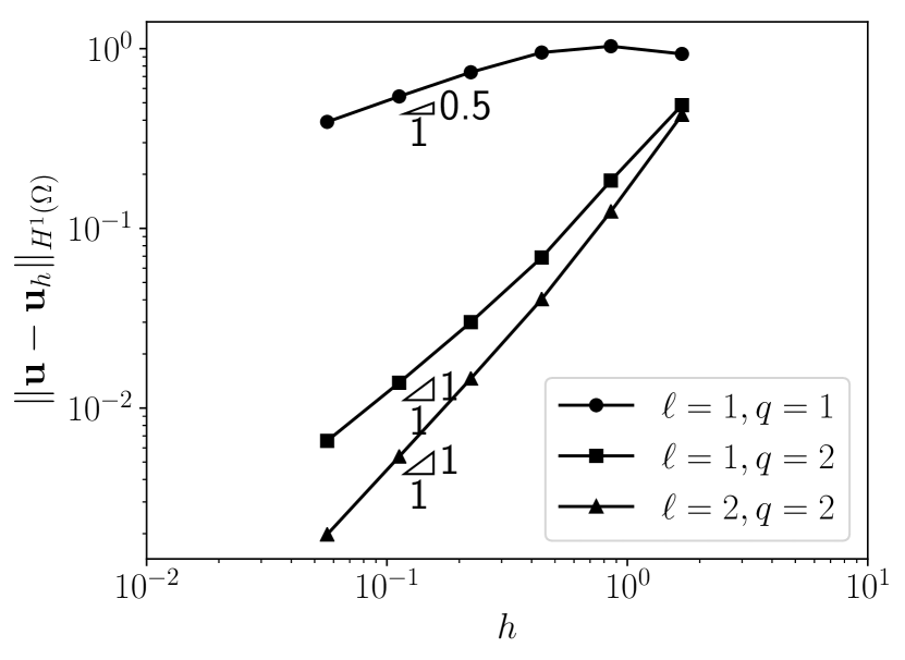
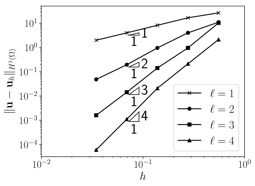
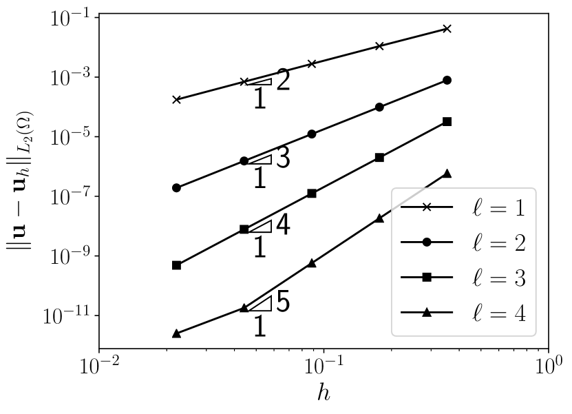
The specification of the numerical fluxes and , when , along with used with the local Lax-Friedrichs flux function within UFL syntax is provided in the code listing presented in Listing 12. Exploiting the software concepts outlined in Section 3 for the automatic computation of DGFEM formulations, the UFL code to construct and solve the resulting DGFEM approximation of (14), (15) is presented in Listing 13, where we have specified that , , and ; thereby, the analytical solution to (14), (15) is given by . We note that on the final line of the code listing given in Listing 13, the call to DOLFIN’s solve function automatically computes the Gâteaux derivative of the DGFEM semilinear form , cf. (6), employed for the numerical approximation of (14), (15) and utilises a Newton solver to evaluate the DGFEM solution; for further details, we refer to [2]. Finally, in Figure 1 we show the asymptotic behaviour of the underlying DGFEM on a sequence of uniformly refined triangular meshes with polynomial orders ; as we expect, we observe that the and norms of the error tend to zero at the respective rates of and as the mesh size tends to zero. The complete code employed for this numerical example is provided in the file advection_diffusion.py.
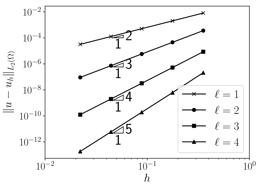
(a)
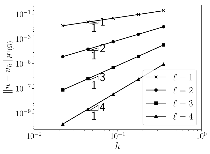
(b)
4.2 Example 2: Compressible Euler Equations
In this second example, we consider the DGFEM discretisation of the compressible Euler equations: find such that
| (16) |
where the convective flux is given by
| (17) |
Here, , , , and denote the density, velocity vector, pressure, and specific total energy, respectively. The equation of state of an ideal gas is given by
where is the ratio of specific heat capacities at constant pressure, , and constant volume, ; for dry air, . Finally, denotes the identity matrix.
The automatic construction of the DGFEM formulation for the numerical approximation of (16) is encapsulated within the class CompressibleEulerOperator. We note that this class simply inherits the HyperbolicOperator class, with the specification of the Euler flux and dissipation parameter required for the definition of the Lax Friedrichs flux, cf. Listing 14 for the case when . We note that in this setting , where is the speed of sound.
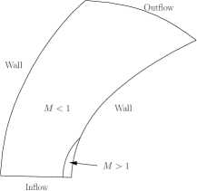
As an illustration of the exploitation of CompressibleEulerOperator, we consider the DGFEM approximation of Ringleb’s flow problem for which an analytical solution may be obtained using the hodograph method, cf. [9]. The DGFEM discretisation of this test case has also been studied in [18]. This problem represents a transonic flow in a curved channel domain, where the flow is mainly subsonic, with a small supersonic region near the right-hand-side wall; cf. Figure 2. Here, inflow/outflow boundary conditions are imposed on the top and bottom boundaries of , while a solid wall condition is specified on the left- and right-hand side boundaries. Following [21] the latter boundary conditions are enforced based on employing a symmetry technique through the specification of the boundary function . More precisely, we treat the walls as part of the Dirichlet boundary, whereby we set
thereby, here and .
(a)
(b)
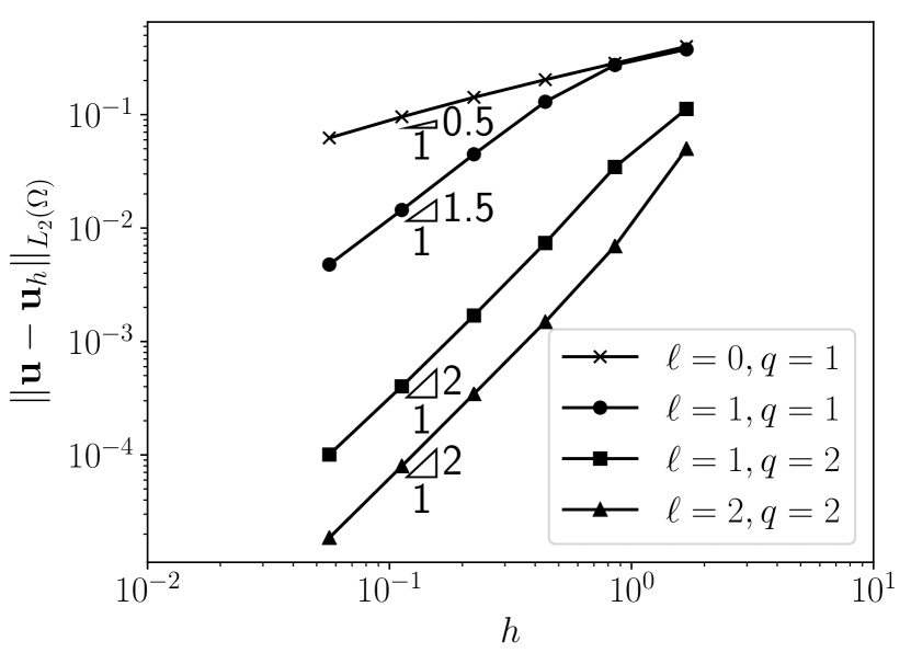
Functions employed for the specification of the analytical solution of Ringleb’s flow, together with routines for the construction of the computational mesh are provided within the file ringleb.py. The curved boundaries on the walls of the domain must be treated in a careful manner to ensure optimal convergence of the underlying DGFEM discretisation. Indeed, our computational experience suggests that a curved polynomial description of the boundary of order is necessary to ensure that the and norms of the error tend to zero at the optimal rates of and as the mesh size tends to zero, for fixed , cf. Figure 3. The complete python code for this numerical example is provided ringleb_example.py; a snippet of this code is depicted in Listing 15 in order to highlight the simplicity of the specification of the DGFEM for this example.
4.3 Example 3a: Compressible Navier-Stokes Equations
In this example we consider the DGFEM discretisation of the compressible Navier-Stokes equations: find such that
| (18) |
where is defined as in (17) and the viscous flux is given by
| (19) |
where denotes the temperature and is the thermal conductivity coefficient. The stress tensor is defined by
where is the dynamic viscosity coefficient. Finally, we note that , where is the Prandtl number.
Given the UFL code in Listing 14, together with the specification of the viscous flux in Listing 16, in the case when , we have implemented the class CompressibleNavierStokesOperator class, which inherits both the CompressibleEuler-Operator and EllipticOperator classes. Indeed, the CompressibleEulerOperator component is treated in an identical manner as in the previous section, while the EllipticOperator component is employed with the UFL specification of the viscous flux. On the basis of these classes, the homogeneity tensor and the resulting symbolic DGFEM formulation can then be automatically generated. Moreover, the Gâteaux derivative of the DGFEM formulation is automatically computed by UFL for use within the Newton solver managed in DOLFIN by invoking the call to solve. As a simple test, we consider the example outlined in [20]; namely, we set and select so that the analytical solution to (4.3) is given by
| (20) |
where . Furthermore, we set , and . The snippet of UFL code required to solve this problem is given in Listing 17; the complete code is provided in compressible_navierstokes_square.py. The orders of convergence of and are reported in Figure 4 as the mesh is uniformly refined for ; as in [20] we observe that and as tends to zero, for each fixed polynomial order .
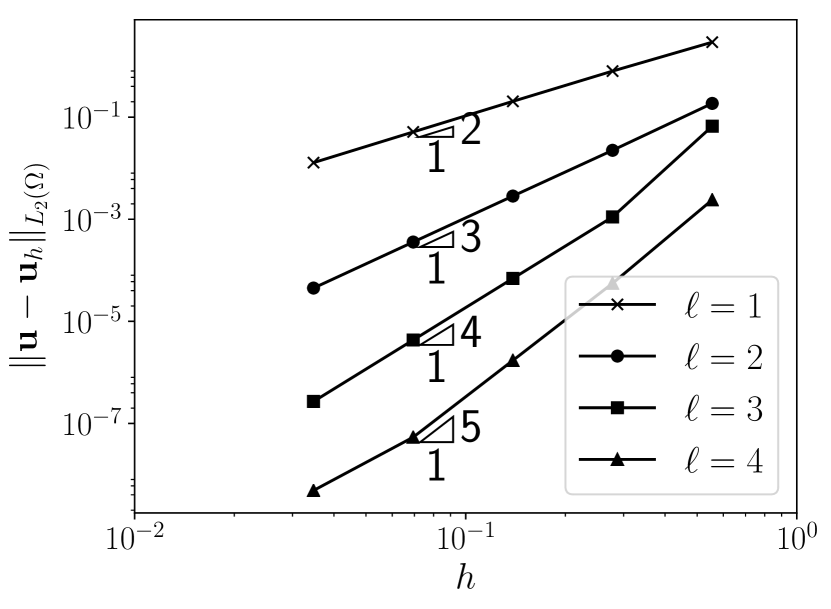
(a)
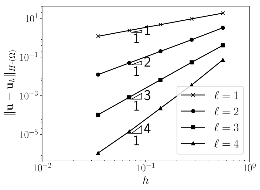
(b)
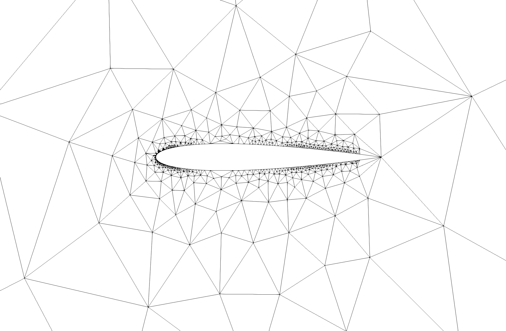
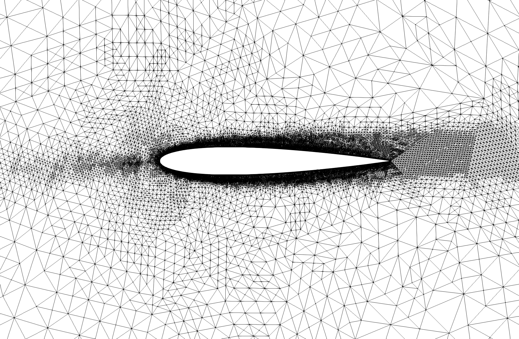
4.4 Example 3b: Compressible Flow Around a NACA0012 Airfoil
To demonstrate the application of the automatic formulation of DGFEMs applied to exterior flow problems, in this section we consider laminar flow around a NACA0012 airfoil whose geometry is defined by
| (21) |
where the thickness fraction . Here, we set the angle of attack , Reynolds number , inlet flow Mach number , and impose an adiabatic no slip condition on the airfoil; cf. [20, 19]. We note that the adiabatic no slip condition imposes a zero heat flux condition on the airfoil surface boundary. We have implemented this by defining a new boundary condition in the class DGAdiabaticWallBC inheriting DGBC. This boundary condition is then recognised by the CompressibleNavierStokesOperator implementation which automatically generates the DGFEM formulation accordingly.
(a)
(b)
(c)
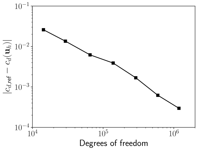
In this example, we shall undertake goal-oriented adaptive mesh refinement based on employing a dual weighted residual (DWR) a posteriori error estimator; for details, we refer to [19]. In particular, we select the quantity of interest to be the drag coefficient
| (22) |
where denotes the surface of the airfoil, , , and denote the far field density and velocity, respectively, and is the reference length scale. The symbolic representation of the underlying dual problem is automatically formulated using the dwr component of dolfin_dg. The error in the approximate drag coefficient on each of the meshes employed is evaluated relative to a reference drag coefficient, computed from a very fine mesh problem. Setting , the convergence of the error in the computed drag coefficient with respect to the number of degrees of freedom in the underlying finite element space, together with the initial and final computational meshes are shown in Figure 5. The code to generate these results is available in the file dg_naca0012_2d.py.
4.5 Example 3c: Entropy Variable Formulation of the Compressible Navier-Stokes Equations
In this section, we consider the DGFEM approximation of the compressible Navier-Stokes equations written in terms of so–called (symmetrisation) entropy variables; for further details, we refer, for example, to [5, 29]. For simplicity of presentation we only consider the two–dimensional case, though the extension to follows in an analogous manner. Thereby, we introduce the change of variable given by
| (23) |
and its inverse
| (24) |
Here, is the internal energy density and is a nondimensional entropy. The implementation of this mapping and its inverse in the UFL symbolic algebra framework is depicted in Listing 18. On the basis of this transformation, the symmetrised formulation of the compressible Navier-Stokes equations is given by: find such that
| (25) |
where and .
(a)
(b)
On the basis of the compressible Euler and compressible Navier-Stokes examples presented in the previous two sections, the DGFEM formulation of problem (25) is straightforward in the symbolic algebra framework of the UFL. We use the convective and viscous fluxes shown in Listings 14 and 16 and implement the transformations (23) and (24) noting that . Indeed, the UFL formulation of the convective and viscous fluxes, and , respectively, are presented in Listing 19. These constructs are then exploited within the DGFEM utility functions in the same manner as in the examples presented in Listings 15 and 17. As a simple test, we consider the numerical approximation of the compressible Navier-Stokes example presented in Section 4.3, based on employing the above entropy variable formulation. To this end, the underlying test problem is first transformed according to the change of variable , cf. (23), whereby the DGFEM is computed; we then transform the numerical solution according to the inverse mapping (24) in order to evaluate the error in the underlying approximation. As in the previous example, we again observe optimal convergence of the underlying DGFEM, cf. Figure 6; the code for this example is provided in Listing 20, cf. compressible_navierstokes_entropy_square.py.
4.6 Example 4: Maxwell Operator
In this penultimate example we demonstrate the extensibility of the symbolic DGFEM framework developed in this article by considering the automatic discretisation of the Maxwell problem: find such that
| (26) | |||||
| (27) |
where, for simplicity, we set and is the wave number; for solvability, we assume that is not a Maxwell eigenvalue. The class MaxwellOperator implements the symmetric interior penalty discretisation of (26), (27) outlined in [27]. Thereby, given the ufl representation of depicted in Listing 21, the corresponding code needed to compute the DGFEM approximation of (26), (27) can be written in the very compact form shown in Listing 22; see maxwell.py. As a simple test case, here we have set , , and such that the analytical solution is given by . Numerical experiments demonstrating the performance of the resulting scheme on a sequence of uniformly refined triangular meshes are presented in Figure 7.
(a)
(b)
4.7 Example 5a: Hyperelasticity
Our final two examples highlight the flexibility of the DGFEM framework proposed in this article for the discretisation of hyperelasticity problems; in this setting DGFEM schemes offer computational benefits in the nearly–incompressible regime, cf. [16, 38]. Given a domain defining an elastic body’s reference configuration with boundary and outward pointing unit normal vector , we seek the displacement vector at all points in the domain which determines the mapping from the reference to the deformed configuration, such that . The constitutive model demands mass balance, so we seek such that
| (28a) | ||||
| (28b) | ||||
| (28c) | ||||
where is the gradient in the reference domain, is the first Piola-Kirchoff stress tensor, is the strain-energy function, is a body force, is the strain tensor, is a traction force, and and denote the Dirichlet and Neumann boundaries, respectively. Here, we examine a neo-Hookean hyperelasticity model where the strain energy density function is given by
where and are the first and second Lamé parameters, respectively, given in terms of Young’s modulus and Poisson ratio .
(a)
(b)
(a)
(b)
(c)
Clearly we observe that equation (28) can be rewritten with , cf. Listing 23; thereby, the DGFEM framework outlined previously may be directly applied. We highlight that the flexibility of this approach naturally allows us to consider other potential strain energy models, such as Saint Venant–Kirchhoff, Ogden, and Mooney–Rivlin [25].
To test the DGFEM solver we repeat the numerical example presented in [33]. To this end, we simulate the small strain deformation of the beam , where , , with the material parameters and . There is no applied body force, i.e., , the beam is clamped on the near face, , , an external distributed force is applied to the far face
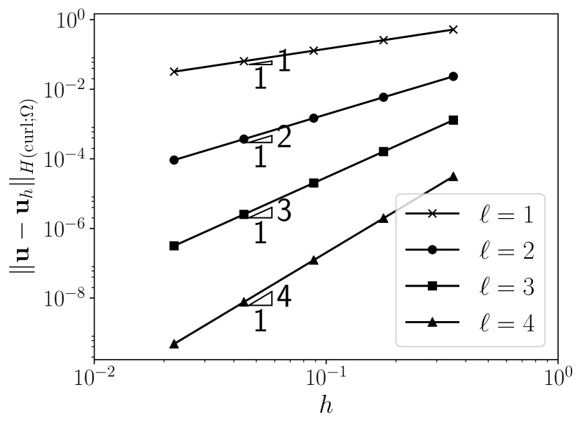
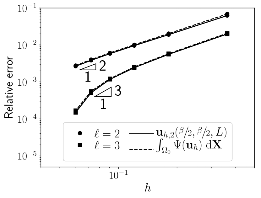
and . The system has a known analytical solution for the tip deflection and the internal strain energy . Convergence of the relative errors of the DGFEM approximation of this problem are shown in Figure 8. The code to generate these results is available in the file dg_cantilever.py.
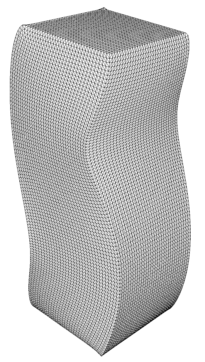
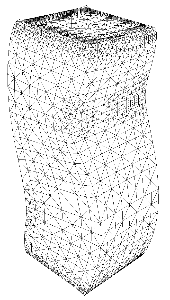
4.8 Example 5b: Near–Incompressible Hyperelastic Buckling
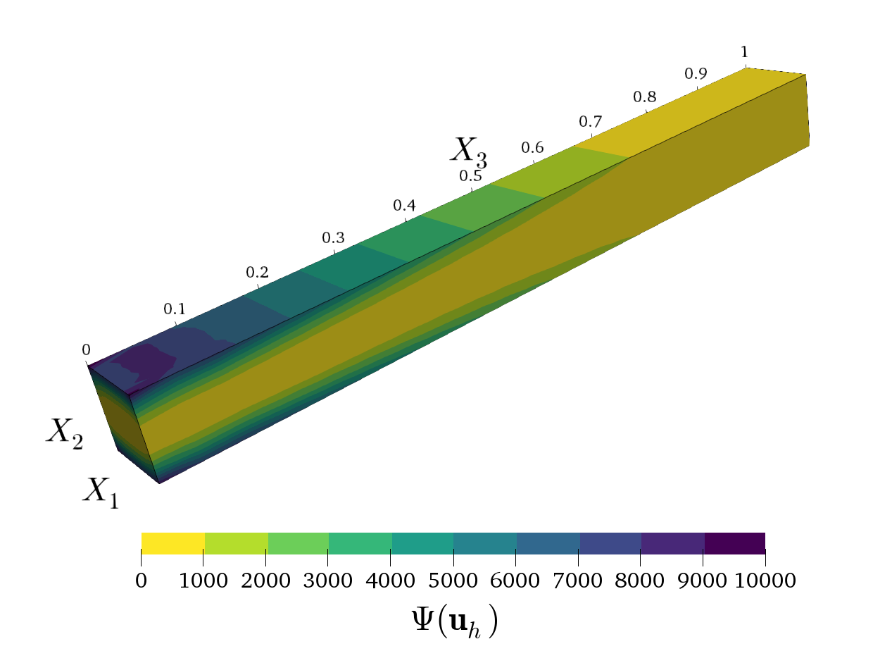
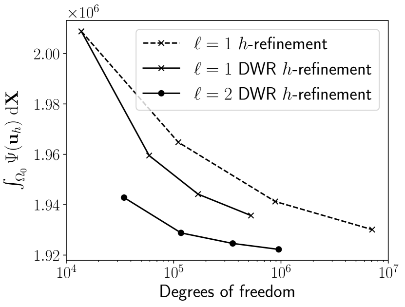
To demonstrate the capability of the DGFEM framework applied to larger three–dimensional problems we draw inspiration from a numerical example of an elastic body buckled in a compressive state, cf. Section 6.7 in [38]. Thereby, we set , , , and prescribe and . Using the proposed DGFEM framework the resulting deformed mesh configuration is shown in Figure 9. Here, we have employed both uniform mesh refinement, as well as adaptive refinement of the computational mesh based on employing a DWR a posteriori error indicator, where we select the internal strain energy to be the quantity of interest. As expected, the adaptive refinement algorithm selects regions to enrich the computational mesh near the edges of the Dirichlet boundary, where large changes in the stress occur, as well as regions under compression, which lead to large changes in the internal strain energy. The implementation of this example is provided in the file dg_compression.py.
5 Concluding remarks
In this article we have exploited the use of symbolic algebra for the automatic computation of DGFEMs for the numerical approximation of general systems of nonlinear PDEs. In particular, we have proposed and implemented a class structure in order to allow for the specification of a given DGFEM in a clear and concise manner. While the examples we have presented have primarily focused on flow problems, we stress that the generality of this approach allows for the treatment of a wide range of PDEs stemming from diverse application areas. Indeed, in the final two examples, we have included the DGFEM approximation of the indefinite Maxwell problem and a hyperelasticity problem, respectively. The exploitation of the software developed within this article allows the user to build up the DGFEM discretisation of systems of multi-physics PDEs in a simple and concise manner; as an example, we have employed the software here for the DGFEM approximation of microwave power assisted chemical vapour deposition reactor employed for the manufacture of synthetic diamond; see [28, 36]. Moreover, the code can easily be extended to other problems, and indeed other DGFEM schemes, so that users can tailor the software to their own applications.
References
- [1] M.S. Alnæs, J. Blechta, J. Hake, A. Johansson, B. Kehlet, A. Logg, C. Richardson, J. Ring, M.E. Rognes, and G.N. Wells, The FEniCS project version 1.5, Arch. Numer. Software 3 (2015), no. 100, 9–23.
- [2] M.S. Alnæs and K.-A. Mardal, SyFi and SFC: Symbolic finite elements and form compilation, Automated Solution of Differential Equations by the Finite Element Method (A. Logg, K.-A. Mardal, and G.N. Wells, eds.), Lecture Notes in Computational Science and Engineering, vol. 84, Springer, 2012, pp. 269–278.
- [3] D.N. Arnold, F. Brezzi, B. Cockburn, and L.D. Marini, Unified analysis of discontinuous Galerkin methods for elliptic problems, SIAM J. Numer. Anal. 39 (2001), 1749–1779.
- [4] W. Bangerth, R. Hartmann, and G. Kanschat, deal.II – a general purpose object oriented finite element library, ACM T. Math. Software 33 (2007), no. 4, 24/1–24/27.
- [5] T.J. Barth, Numerical methods for gasdynamic systems on unstructured meshes, An Introduction to Recent Developments in Theory and Numerics for Conservation Laws (D. Kröner, M. Ohlberger, and C. Rohde, eds.), Lecture Notes in Computational Science and Engineering, vol. 5, Springer, 1999, pp. 195–285.
- [6] Francesco Bassi, Stefano Rebay, G. Mariotti, S. Pedinotti, and M. Savini, A high-order accurate discontinuous finite element method for inviscid and viscous turbomachinery flows, 2nd European Conference on Turbomachinery Fluid Dynamics and Thermodynamics, Antwerpen, Belgium, March 5–7, 1997 (R. Decuypere and G. Dibelius, eds.), Technologisch Instituut, 1997, pp. 99–108.
- [7] S.J. Berkowitz, On computing the determinant in small parallel time using a small number of processors, Information Processing Letters 18 (1984), no. 3, 147–150.
- [8] M. Blatt, A. Burchardt, A. Dedner, C. Engwer, J. Fahlke, B. Flemisch, C. Gersbacher, C. Gräser, F. Gruber, C. Grüninger, D. Kempf, R. Klöfkorn, T. Malkmus, S. Müthing, M. Nolte, M. Piatkowski, and O. Sander, The distributed and unified numerics environment, version 2.4, Arch. Numer. Software 4 (2016), no. 100, 13–29.
- [9] G. Chiocchia, Exact solutions to transonic and supersonic flows, AGARD (1985), AR–211.
- [10] K.A. Cliffe, A. Spence, and S.J. Tavener, The numerical analysis of bifurcation problems with application to fluid mechanics, Acta Numerica (A. Iserles, ed.), vol. 9, Cambridge University Press, 2000, p. 39–131.
- [11] K.A. Cliffe and S.J. Tavener, Implementation of extended systems using symbolic algebra, Continuation Methods in Fluid Dynamics, Notes on Numerical Fluid Mechanics, 2000, pp. 81–92.
- [12] B. Cockburn, An introduction to the discontinuous Galerkin method for convection-dominated problems, Advanced numerical approximation of nonlinear hyperbolic equations (Cetraro, 1997), Springer, Berlin, 1998, pp. 151–268. MR 1 728 854
- [13] B. Cockburn, G.E. Karniadakis, and C.-W. Shu (eds.), Discontinuous Galerkin methods, Springer-Verlag, Berlin, 2000, Theory, computation and applications, Papers from the 1st International Symposium held in Newport, RI, May 24–26, 1999.
- [14] D.A. Di Pietro and A. Ern, Mathematical aspects of discontinuous Galerkin methods, Mathématiques & Applications (Berlin) [Mathematics & Applications], vol. 69, Springer, Heidelberg, 2012.
- [15] E.H. Georgoulis, E. Hall, and P. Houston, Discontinuous Galerkin methods on –anisotropic meshes II: A posteriori error analysis and adaptivity, Appl. Numer. Math. 59(9) (2009), 2179–2194.
- [16] P. Hansbo and M. G. Larson, Discontinuous Galerkin methods for incompressible and nearly incompressible elasticity by Nitsche’s method, Comput. Methods Appl. Mech. Engrg. 191 (2002), no. 17, 1895 – 1908.
- [17] R. Hartmann and P. Houston, Adaptive discontinuous Galerkin finite element methods for nonlinear hyperbolic conservation laws, SIAM J. Sci. Comput. 24 (2002), 979–1004.
- [18] R. Hartmann and P. Houston, Adaptive discontinuous Galerkin finite element methods for the compressible Euler equations, J. Comput. Phys. 183 (2002), no. 2, 508–532.
- [19] , Symmetric interior penalty DG methods for the compressible Navier-Stokes equations I: Method formulation, International Journal of Numerical Analysis and Modeling 3 (2005), no. 1, 1–20.
- [20] R. Hartmann and P. Houston, An optimal order interior penalty discontinuous Galerkin discretization of the compressible Navier–Stokes equations, J. Comput. Phys. 227 (2008), no. 22, 9670–9685.
- [21] , Error estimation and adaptive mesh refinement for aerodynamic flows, VKI LS 2010-01: 36th CFD/ADIGMA Course on -Adaptive and -Multigrid Methods, Oct. 26-30, 2009 (H. Deconinck, ed.), Von Karman Institute for Fluid Dynamics, Belgium, 2010.
- [22] A.C. Hearn, Reduce user’s manual version 3.8, 2004.
- [23] F. Hecht, New development in FreeFem++, J. Numer. Math. 20 (2012), no. 3-4, 251–265.
- [24] J.S. Hesthaven and T. Warburton, Nodal discontinuous Galerkin methods, Texts in Applied Mathematics, vol. 54, Springer, New York, 2008, Algorithms, analysis, and applications.
- [25] G. A. Holzapfel, Nonlinear solid mechanics: A continuum approach for engineering, Wiley, 2000.
- [26] P. Houston, AptoFEM finite element analysis software, 2015.
- [27] P. Houston, I. Perugia, A. Schneebeli, and D. Schötzau, Interior penalty method for the indefinite time-harmonic Maxwell equations, Numer. Math. 100 (2005), no. 3, 485–518.
- [28] P. Houston and N. Sime, Numerical modelling of MPA-CVD reactors with the discontinuous Galerkin finite element method, J. Phys. D: Appl. Phys. 50 (2017), no. 29, 295202.
- [29] T.J.R. Hughes, L.P. Franca, and M. Mallet, A new finite element formulation for computational fluid dynamics: I. symmetric forms of the compressible Euler and Navier-Stokes equations and the second law of thermodynamics, J. Comput. Phys. 54 (1986), 223–234.
- [30] D. Kröner, Numerical schemes for conservation laws, Wiley-Teubner, 1997.
- [31] A. Logg, K.A. Mardal, and G. Wells, Automated Solution of Differential Equations by the Finite Element Method: The FEniCS Book (Lecture Notes in Computational Science and Engineering), Springer, 2012.
- [32] G.R. Markall, D.A. Ham, and P.H.J. Kelly, Towards generating optimised finite element solvers for GPUs from high-level specifications, Proc. Comp. Sci. 1 (2010), no. 1, 1815 – 1823.
- [33] L. Noels and R. Radovitzky, A general discontinuous Galerkin method for finite hyperelasticity. formulation and numerical applications, Internat. J. Numer. Methods Engrg. 68 (2006), no. 1, 64–97.
- [34] K. Ølgaard, Automated computational modelling for complicated partial differential equations, Ph.D. thesis, Technische Universiteit Delft, 2013.
- [35] B. Rivière, Discontinuous Galerkin methods for solving elliptic and parabolic equations, Frontiers in Applied Mathematics, vol. 35, Society for Industrial and Applied Mathematics (SIAM), Philadelphia, PA, 2008, Theory and implementation.
- [36] N. Sime, Numerical modelling of chemical vapour deposition reactors, Ph.D. thesis, University of Nottingham, 2016.
- [37] SymPy Development Team, Sympy: Python library for symbolic mathematics, 2014.
- [38] A. Ten Eyck and A. Lew, Discontinuous Galerkin methods for non-linear elasticity, Internat. J. Numer. Methods Engrg. 67 (2006), no. 9, 1204–1243.
- [39] E.F. Toro, Riemann solvers and numerical methods for fluid dynamics, Springer, 1997.
- [40] H.G. Weller and G. Tabor, A tensorial approach to computational continuum mechanics using object-oriented techniques, Comput. Phys. 12 (1998), no. 6, 620–631.