Adaptive Cost-Sensitive Online Classification

Abstract

Cost-Sensitive Online Classification has drawn extensive attention in recent years, where the main approach is to directly online optimize two well-known cost-sensitive metrics: (i) weighted sum of sensitivity and specificity; (ii) weighted misclassification cost. However, previous existing methods only considered first-order information of data stream. It is insufficient in practice, since many recent studies have proved that incorporating second-order information enhances the prediction performance of classification models. Thus, we propose a family of cost-sensitive online classification algorithms with adaptive regularization in this paper. We theoretically analyze the proposed algorithms and empirically validate their effectiveness and properties in extensive experiments. Then, for better trade off between the performance and efficiency, we further introduce the sketching technique into our algorithms, which significantly accelerates the computational speed with quite slight performance loss. Finally, we apply our algorithms to tackle several online anomaly detection tasks from real world. Promising results prove that the proposed algorithms are effective and efficient in solving cost-sensitive online classification problems in various real-world domains.

Abstract

This supplemental file provides the proofs of theorems and the related work in our paper of ”Adaptive Cost-Sensitive Online Classification”.

1 Introduction

With the rapid growth of datasets, the technologies of machine learning and data mining power many respects of modern society: from content filtering to web searches on social networks, and from goods recommendations to intelligent customer services on e-commerce. Gradually, many real-world large-scale applications make use of a family of techniques called online learning, which has been extensively studied for many years in machine learning and data mining literatures[25, 35, 36, 4, 5, 6]. In general, online learning is a class of efficient and scalable machine learning methods, whose goal is to incrementally learn a model to make correct predictions on a stream of samples. This family of methods provides an opportunity to solve many real-world applications that data arrives sequentially while predictions must be made instantly, such as malicious URL detection[4, 7] and portfolio selection[8]. In addition, online learning is also good at solving large-scale learning tasks, e.g., learning support vector machine from billions of data[9].

However, although online learning was studied widely, most existing methods were inappropriate to solve cost-sensitive classification problems, because most of them seek performance based on measurable accuracy or mistake rate, which are obviously cost-insensitive. As a result, these algorithms are difficult to handle numerous real-world problems, where datasets are always class-imbalanced, i.e., the mistake costs of samples are significantly different[9, 11, 12]. To solve this problem, researchers have suggested to use more meaningful metrics, such as the weighted sum of sensitivity and specificity[6, 7], and the weighted misclassification cost[9, 8] to replace old ones. Based on this, many batch classification algorithms are proposed to directly optimize prediction performance for cost-sensitive classification over the past decades[9, 8]. However, these batch algorithms often suffer from poor scalability and efficiency for large-scale tasks, which make them inappropriate for online classification applications.

Although both online classification and cost-sensitive classification were studied widely, quite few literatures study cost-sensitive online classification. As results, the Cost-Sensitive Online Classification framework[15, 16] was recently proposed to fill the gap between online learning and cost-sensitive classification. According to this framework, a class of algorithms named as Cost-Sensitive Online Gradient Descend (COG) was proposed to directly optimize predefined cost-sensitive metrics (e.g., weighted sum or weighted misclassification cost) based on online gradient descent technique. Particularly, compared with other traditional online algorithms, COG shows strong empirical performance in solving cost-sensitive online classification problems.

However, although COG is able to handle the Cost-sensitive online classification tasks, it only takes the first order information of samples (i.e., weighted mean of the gradient). It is obviously insufficient, since many recent studies[36, 31, 32, 33] have shown that comprehensive consideration with second-order information (i.e., the correlations between features) significantly enhances the performance of online classification.

As an attempt to remedy the limitation of first-order approaches, we propose the Adaptive Regularized Cost-Sensitive Online Gradient Descent algorithms (named ACOG), based on the state-of-the-art Confidence Weighted strategy[36, 31, 32, 33]. We theoretically analyze their regret bounds[21] and their cost-sensitive metric bounds. Corresponding conclusions confirm the good convergence of ACOG algorithms.

Furthermore, although enjoying the advantage of second-order information, our proposed algorithms are at the cost of higher running time, because the updating process of correlation matrix is time-consuming. As results, it may be inappropriate for some real-world applications with quite high-dimensional datasets. Thus, for better trade off between the efficiency and performance, we further propose an updated version of ACOG algorithms based on sketching techniques[44, 23, 24, 25], whose running time is linear in the dimensions of samples, just like the first order methods.

Next, we conduct extensive experiments to evaluate the performance and specialities of our proposed algorithms and then apply them to solve online anomaly detection tasks from several real-world domains. Promising results confirm the effectiveness and efficiency of our methods in real-world cost-sensitive online classification problems.

Note that a brief version of this paper had been published in the IEEE ICDM conference[26]. Compared with it, this journal manuscript makes several significant extensions, including (1) an updated variant with sketching methods and some theoretical analyses about its time complexity; (2) an extension of ACOG with an additional loss function and theoretical analyses; (3) more extensive empirical studies to evaluate the proposed algorithms.

The rest of this paper is organized as follows. We present the problem formulation and the proposed algorithms with theoretical analyses in section 2. To save space, we provide theorem proofs and related work in supplemental materials. Next, we propose an efficient version based on sketching techniques in section 3. After that, section 4 empirically evaluates the performance and properties of our algorithms, and section 5 shows an application to real-world anomaly detection tasks. Finally, section 6 concludes the paper.

2 Setup and Algorithm

In this section, we firstly introduce the framework and formulation setting of the Cost-Sensitive Online Classification problem[15, 16]. Then, we present the proposed Adaptively Regularized Cost-Sensitive Online Gradient Descent algorithms (ACOG) in detail.

2.1 Problem Setting

Without loss of generality, we consider online binary classification problems here. The main goal is to learn a linear classification model with an updatable predictive vector $w\in\mathbb{R}^{d}$, based on a stream of training samples $\{(x_{1},y_{1}),(x_{2},y_{2}),...,(x_{T},y_{T})\}$, where $T$ is the total quantity of samples, $x_{t}\in\mathbb{R}^{d}$ is the $d$-dimensional sample at time $t$, and $y_{t}\in\{-1,1\}$ is the corresponding true class label. In detail, at the $t$-th round of learning, the learner obtains a sample $x_{t}$ and then predicts its estimated class label $\hat{y}_{t}={\rm sign}(w_{t}^{\top}x_{t})$, where $w_{t}$ is the model predictive vector learnt from the previous $t-1$ samples. Then, the model receives the ground truth of instance $y_{t}\in\{-1,1\}$, which is the label of true class. If $\hat{y}_{t}=y_{t}$, the model makes a correct prediction; otherwise, it makes a mistake and suffers a loss. In the end, the learner updates its predictive vector $w_{t}$ based on the received painful loss.

For convenience, we define $\mathcal{M}=\{t\ |y_{t}\neq{\rm sign}(w_{t}\cdot x_{t}),\forall t\in[T]\}$ is the mistake index set, $\mathcal{M}_{p}=\{t\in\mathcal{M}$ and $y_{t}=+1\}$ is the positive set of mistake index and $\mathcal{M}_{n}=\{t\in\mathcal{M}$ and $y_{t}=-1\}$ is the negative one. In addition, we set $M=|\mathcal{M}|$, $M_{p}=|\mathcal{M}_{p}|$ and $M_{n}=|\mathcal{M}_{n}|$ to denote the number of total mistakes, positive mistakes and negative mistakes. Moreover, we denote the index sets of all positive samples and all negative samples by $\mathcal{I}^{p}_{T}=\{i\in[T]|y_{i}=+1\}$ and $\mathcal{I}^{n}_{T}=\{i\in[T]|y_{i}=-1\}$, where $T_{p}=|\mathcal{I}^{p}_{T}|$ and $T_{n}=|\mathcal{I}^{n}_{T}|$ denote the number of positive samples and negative samples.

For performance metrics of this problem, we first assume the positive samples as rare class, i.e., $T_{p}\leq T_{n}$. Generally, traditional online classification approaches are eager to maximize accuracy (or minimize mistake rate equivalently):

$$accuracy=\frac{T-M}{T}.$$

However, this metric is inappropriate for imbalanced data, because models can easily obtain high accuracy, even simply classifying all imbalanced samples as negative class. So, a more suitable approach is to measure the $sum$ of weighted $sensitivity$ and $specificity$:

$$sum=\alpha_{p}\times\frac{T_{p}-M_{p}}{T_{p}}+\alpha_{n}\times\frac{T_{n}-M_{n}}{T_{n}},$$

where $\alpha_{p},\alpha_{n}\in[0,1]$ are weight parameters for trade off between sensitivity and specificity, and $\alpha_{p}+\alpha_{n}=1$. Note that if $\alpha_{p}=\alpha_{n}=0.5$, the $sum$ metric becomes the famous balanced $accuracy$ metric.

In addition, another metric to measure is the misclassification $cost$ suffered by the model:

$$cost=c_{p}\times M_{p}+c_{n}\times M_{n},$$

where $c_{p},c_{n}\in[0,1]$ are misclassification cost parameters for positive and negative instances, and $c_{p}+c_{n}=1$. Generally, either the higher of the $sum$ value or the lower of the $cost$ value, the better performance of classification.

Then, we can adjust our focus to maximize $sum$ metric or minimize $cost$ metric. As is known in [15, 16], both objectives are equivalent to minimizing the following objective:

$$\sum_{y_{t}=+1}\rho\mathbb{I}_{(y_{t}w\cdot x_{t}<0)}+\sum_{y_{t}=-1}\mathbb{I}_{(y_{t}w\cdot x_{t}<0)},$$ (1)

where $\rho=\frac{\alpha_{p}T_{n}}{\alpha_{n}T_{p}}$ for weighted $sum$ metric and $\rho=\frac{c_{p}}{c_{n}}$ for weighted $cost$ metric.

2.2 Algorithm

In this subsection, we present the proposed ACOG algorithms by optimizing the objective from Eq. (1). However, this objective function is non-convex. Thus, to facilitate the optimization, we replace the indicator function with its convex variants (either one of the following two functions):

$$\ell^{I}(w;(x,y))={\rm max}(0,(\rho*\mathbb{I}_{(y=1)}\small{+}\mathbb{I}_{(y=-1)})\small{-}y(w\cdot x)),$$ (2)

$$\ell^{II}(w;(x,y))=(\rho*\mathbb{I}_{(y=1)}\small{+}\mathbb{I}_{(y=-1)})*{\rm max}(0,1\small{-}y(w\cdot x)).$$ (3)

For $\ell^{I}(w;(x,y))$, the change of margin yields more ”frequent” updates for specific class, compared to the traditional hinge loss; while for $\ell^{II}(w;(x,y))$, the change of the slope causes to more ”aggressive” updates for specific class.

Then, our aim is to minimize the regret of learning process[21], based on either loss functions $\ell^{I}(w;(x,y))$ or $\ell^{II}(w;(x,y))$:

$$Regret:=\sum_{t=1}^{T}\ell(w_{t};(x_{t},y_{t}))-\sum_{t=1}^{T}\ell(w^{*};(x_{t},y_{t})),$$ (4)

where $w^{*}={\rm arg\ min}_{t}\sum_{t=1}^{T}\nabla\ell(w;(x_{t},y_{t}))$. To solve this optimization problem, the cost-sensitive online gradient descent algorithms (COG)[15, 16] were proposed:

$$w_{t+1}=w_{t}-\eta\nabla\ell_{t}(w_{t}),$$

where $\eta$ is the learning rate and $\ell_{t}(w_{t})=\ell(w;(x_{t},y_{t}))$. However, COG algorithms only consider the first order gradient information of the sample stream to update the learner, which is clearly insufficient since many recent studies have shown the significance of incorporating the second order information[36, 31, 32, 33]. Motivated by this discovery, we propose to introduce adaptive regularization to promote the cost-sensitive online classification.

Let us assume the online model satisfies a multivariate Gaussian distribution, i.e., $w\sim\mathcal{N}(\mu,\Sigma)$ , where $\mu$ is the mean value vector of distribution and $\Sigma$ is the covariance matrix of distribution. Then, we can predict the class label of an sample $x$ based on ${\rm sign}(w^{\top}x)$, when given a definite multivariate Gaussian distribution. In reality, it is more practical to make predictions by simply using distribution mean $\mathbb{E}[w]=\mu$ rather than $w$. So, the rule of model prediction actually adopts ${\rm sign}(\mu^{\top}x)$ in the following. For better understanding, each mean value $\mu_{i}$ can be regarded as the model’s knowledge about the feature $i$; while the diagonal entry of covariance matrix $\Sigma_{i,i}$ is regarded as the confidence of feature $i$. Generally, the smaller of $\Sigma_{i,i}$, the more confidence in the mean weight $\mu_{i}$ for feature $i$. In addition to diagonal values, other covariance terms $\Sigma_{i,j}$ can be understood as the correlations between two mean weight value $\mu_{i}$ and $\mu_{j}$ for feature $i$ and $j$.

Given a multivariate Gaussian distribution, we naturally recast the object functions by minimizing the following unconstraint objective, based on the divergence between empirical distribution and probability distribution:

$$D_{KL}(\mathcal{N}(\mu,\Sigma)||\mathcal{N}(\mu_{t},\Sigma_{t}))+\eta\ell_{t}(\mu)+\frac{1}{2\gamma}x_{t}^{\top}\Sigma x_{t},$$

where $D_{KL}$ is the Kullback-Leibler divergence, $\eta$ is fitting parameter and $\gamma$ is regularized parameter. Specifically, this objective helps to reach trade off between distribution divergence (first term), loss function (second term) and model confidence (third term). In other word, the objective would like to make the least adjustment at each round to minimize the loss and optimize the confidence of model. To solve this optimization problem, we first depict the Kullback-Leibler divergence explicitly:

$$D_{KL}\big{(} \mathcal{N}(\mu,\Sigma)||\mathcal{N}(\mu_{t},\Sigma_{t})\big{)}$$

$$= \frac{1}{2}{\rm log}\Big{(}\frac{{\rm det}\Sigma_{t}}{{\rm det}\Sigma}\Big{)}+\frac{1}{2}{\rm Tr}(\Sigma^{-1}_{t}\Sigma)+\frac{1}{2}||\mu_{t}-\mu||_{\Sigma^{-1}_{t}}^{2}-\frac{d}{2}.$$

However, this optimization function dose not have the closed-form solution. Thus, we change the loss term $\ell_{t}(\mu)$ with its first order Taylor expansion $\ell_{t}(\mu_{t})+g_{t}^{\top}(\mu-\mu_{t})$, where $g_{t}=\partial\ell_{t}(\mu_{t})$. Now, we obtain the final optimization objective by removing constant terms:

$$f_{t}(\mu,\Sigma)=D_{KL}(\mathcal{N}(\mu,\Sigma)||\mathcal{N}(\mu_{t},\Sigma_{t}))\small{+}\eta g_{t}^{\top}\mu\small{+}\frac{1}{2\gamma}x_{t}^{\top}\Sigma x_{t},$$ (5)

which is much easier to be solved.

A simple method to solve this objective function is to decompose it into two parts depending on $\mu$ and $\Sigma$, respectively. Then, the updates of mean vector $\mu$ and covariance matrix $\Sigma$ can be performed independently:

$\bullet$     Update the mean parameter:

$$\mu_{t+1}={\rm arg}\ \min_{\mu}f_{t}(\mu,\Sigma);$$

$\bullet$     If $\ell_{t}(\mu_{t})\neq 0$, update the covariance matrix:

$$\Sigma_{t+1}={\rm arg}\ \min_{\Sigma}f_{t}(\mu,\Sigma).$$

For the update of mean parameter, setting the derivative of $\partial_{\mu}f_{t}(\mu_{t+1},\Sigma)$ as zero will give:

$$\Sigma_{t}^{-1}(\mu_{t+1}-\mu_{t})+\eta g_{t}=0\hskip 4.30554pt\Longrightarrow\hskip 4.30554pt\mu_{t+1}=\mu_{t}-\eta\Sigma_{t}g_{t},$$

while for covariance matrix, setting the derivative of $\partial_{\Sigma}f_{t}(\mu,\Sigma_{t+1})$ as zero will result in:

$$-\Sigma_{t+1}^{-1}+\Sigma_{t}^{-1}+\frac{x_{t}x_{t}^{\top}}{\gamma}=0\hskip 4.30554pt\Longrightarrow\hskip 4.30554pt\Sigma_{t+1}^{-1}=\Sigma_{t}^{-1}+\frac{x_{t}x_{t}^{\top}}{\gamma},$$

where adopting the Woodbury identity[28] will give:

$$\Sigma_{t+1}=\Sigma_{t}-\frac{\Sigma_{t}x_{t}x_{t}^{\top}\Sigma_{t}}{\gamma+x_{t}^{\top}\Sigma_{t}x_{t}}.$$ (6)

Note that the update of mean parameter $\mu$ relies on the confidence parameter $\Sigma$, we thus propose to update $\mu$ based on the updated covariance matrix $\Sigma_{t+1}$ instead of the old one $\Sigma_{t}$, which should be more accurate:

$$\mu_{t+1}=\mu_{t}-\eta\Sigma_{t+1}g_{t}.$$ (7)

This is different from AROW[32], where the updating rule of $\mu_{t}$ based on the old matrix $\Sigma_{t}$. To intuitively understand this change, let us assume $\Sigma_{t+1}$ as a diagonal matrix. Then, we can find that the updating process actually assigns the updating value of each dimension with different self-adaptive learning rates. So, it is more appropriate to update $\mu$, with the learning rate that considers the current sample. In other words, the more unconfident of the weight, the more aggressive of its updates. Then, we summarize the proposed Adaptive Regularized Cost-Sensitive Online Gradient Descent (ACOG) in Alogrithm 1.

Algorithm 1 Adaptive Regularized Cost-Sensitive Online Gradient Descent (ACOG)

1:learning rate $\eta$; regularized parameter $\gamma$; bias parameter $\rho=\frac{\alpha_{p}*T_{n}}{\alpha_{n}*T_{p}}$ for “sum“ and $\rho=\frac{c_{p}}{c_{n}}$ for “cost“.

2:$\mu_{1}=0$, $\Sigma_{1}=I$.

3:for $t=1\to T$ do

4:     Receive sample $x_{t};$

5:     Compute $\ell_{t}(\mu_{t})\small{=}\ell^{*}(\mu_{t};(x_{t},y_{t})),where\ *\in\{I,II\};$

6:     if $\ell_{t}(\mu_{t})>0$ then

7:         $\Sigma_{t+1}=\Sigma_{t}-\frac{\Sigma_{t}x_{t}x_{t}^{\top}\Sigma_{t}}{\gamma+x_{t}^{\top}\Sigma_{t}x_{t}};$

8:         $\mu_{t+1}=\mu_{t}-\eta\Sigma_{t+1}g_{t},\ where\ g_{t}=\partial_{\mu}\ell_{t}(\mu_{t});$

9:     else

10:         $\mu_{t+1}=\mu_{t},\Sigma_{t+1}=\Sigma_{t};$

11:     end if

12:end for

For simplification, we ignore the sample numbers $T$ in the analyses of algorithms efficiency. Thus the time complexity for the updates of $\Sigma_{t+1}$ and $\mu$ are both $\mathcal{O}(d^{2})$, so the overall time complexity for ACOG is $\mathcal{O}(d^{2})$, which is quite slower than the first order COG algorithms, especially for high-dimensional datasets. To reduce the time complexity, We propose to use the diagonal version of ACOG (i.e., ACOG_diag), which accelerates the speed of ACOG algorithms to $\mathcal{O}(d)$. Specifically, only a diagonal version $\Sigma_{t}$ would be maintained and updated at round $t$, which can improve computational efficiency and save memory cost.

Remark. In ACOG algorithms, one practical concern is the setting of the value of $\rho$, when optimizing the weighted $sum$ performance. Normally, $\rho$ is denoted as $\rho=\frac{\alpha_{p}T_{n}}{\alpha_{n}T_{p}}$ for $sum$ metric. However, the value of $T_{p}$ and $T_{n}$ might be unknown in advance on real-world online classification tasks. A practical method is to approximate the ratio $\frac{T_{n}}{T_{p}}$ according to the empirical distribution of the past training instances, and adaptively update $\frac{T_{n}}{T_{p}}$ during the online learning process. In addition, we would empirical examine this problem in experiments.

2.3 Theoretical Analysis

In this subsection, we theoretically analyze the proposed ACOG algorithms in terms of two cost-sensitive metrics. Before that, we first prove an important theorem, which gives the regret bounds for algorithms that contributes to later theoretical analyses.

Theorem 1.  Let $(x_{1},y_{1}),(x_{2},y_{2}),...,(x_{T},y_{T})$ be a sequence of samples, where $x_{t}\in\mathbb{R}^{d},y_{t}\in\{-1,1\}$. Then for any $\mu\in\mathbb{R}^{d}$, by setting $\eta=\sqrt{\frac{{\rm max}_{t\leq T}||\mu_{t}-\mu||^{2}{\rm Tr}(\Sigma_{T+1}^{-1})}{\gamma{\rm log}(|\Sigma_{T+1}^{-1}|)}}$, the proposed ACOG-I satisfies:

$$Regret\leq D_{\mu}\sqrt{\gamma{\rm Tr}(\Sigma_{T+1}^{-1}){\rm log}(|\Sigma_{T+1}^{-1}|)},$$

where $D_{\mu}={\rm max}_{t}||\mu_{t}-\mu||$. In addition, by setting $\eta=\sqrt{\frac{{\rm max}_{t\leq T}||\mu_{t}-\mu||^{2}{\rm Tr}(\Sigma_{T+1}^{-1})}{\rho^{2}\gamma{\rm log}(|\Sigma_{T+1}^{-1}|)}}$, ACOG-II satisfies:

$$Regret\leq\rho D_{\mu}\sqrt{\gamma{\rm Tr}(\Sigma_{T+1}^{-1}){\rm log}(|\Sigma_{T+1}^{-1}|)}.$$

Remark. Let us suppose $||x_{t}||\leq 1$, it is easy to discover ${\rm Tr}(\Sigma_{T+1}^{-1})\leq O(T/\gamma)$, which means the regrets of ACOG are in the order of $O(\sqrt{T})$. This order of regret is the optimal, since the loss function is not strongly convex[43].

Theorem 2.  Under the same assumptions in the Theorem 1, by setting $\rho=\frac{\alpha_{p}T_{n}}{\alpha_{n}T_{p}}$, for any $\mu\in\mathbb{R}^{d}$ the ACOG-I satisfies:

$$sum\geq 1\small{-}\frac{\alpha_{n}}{T_{n}}[\sum_{t=1}^{T}\ell_{t}(\mu)\small{+}D_{\mu}\sqrt{\gamma{\rm Tr}(\Sigma_{T+1}^{-1}){\rm log}(|\Sigma_{T+1}^{-1}|)}],$$

and the ACOG-II satisfies:

$$sum\geq 1\small{-}\frac{\alpha_{n}}{T_{n}}[\sum_{t=1}^{T}\ell_{t}(\mu)\small{+}\rho D_{\mu}\sqrt{\gamma{\rm Tr}(\Sigma_{T+1}^{-1}){\rm log}(|\Sigma_{T+1}^{-1}|)}].$$

Remark. It is easy to verify that $\sum_{t=1}^{T}\ell_{t}(\mu)$ is a convex estimate of $\rho M_{p}+M_{n}$ for $\mu$, so $\frac{\alpha_{n}}{T_{n}}\sum_{t=1}^{T}\ell_{t}(\mu)$ is an estimate of $\alpha_{p}\frac{M_{p}}{T_{p}}+\alpha_{n}\frac{M_{n}}{T_{n}}$. In addition, it is worthy noting that $\alpha_{n}$ cannot be set as zero, since $\rho=\frac{\alpha_{p}T_{n}}{\alpha_{n}T_{p}}$. However, one limitation here is that we may not know $\frac{T_{n}}{T_{p}}$ in advance for a real-world online learning task. To solve this issue, an alternative approach is to consider the $cost$ metric, which does not need the $\frac{T_{n}}{T_{p}}$ term in advance because $\rho=\frac{c_{p}}{c_{n}}$.

Theorem 3.  Under the same assumptions in the Theorem 1, by setting $\rho=\frac{c_{p}}{c_{n}}$, for any $\mu\in\mathbb{R}^{d}$, the ACOG-I satisfies:

$$cost\leq c_{n}[\sum_{t=1}^{T}\ell_{t}(\mu)\small{+}D_{\mu}\sqrt{\gamma{\rm Tr}(\Sigma_{T+1}^{-1}){\rm log}(|\Sigma_{T+1}^{-1}|)}],$$

and the ACOG-II satisfies:

$$cost\leq c_{n}[\sum_{t=1}^{T}\ell_{t}(\mu)\small{+}\rho D_{\mu}\sqrt{\gamma{\rm Tr}(\Sigma_{T+1}^{-1}){\rm log}(|\Sigma_{T+1}^{-1}|)}].$$

Remark. For the $cost$ metric, $\sum_{t=1}^{T}\ell_{t}(\mu)$ is a convex estimate of $\frac{c_{p}}{c_{n}}M_{p}+M_{n}$, and so $c_{n}\sum_{t=1}^{T}\ell_{t}(\mu)$ is an estimate of $c_{p}M_{p}+c_{n}M_{n}$. Moreover, one should note that $c_{n}$ cannot be set as zero because of $\rho=\frac{c_{p}}{c_{n}}$.

3 Enhanced Algorithm with Sketching

As mentioned above, the time complexity of ACOG is $O(d^{2})$ and its diagonal version is $O(d)$. However, the diagonal ACOG cannot enjoy the correlation information between different dimensions of samples. When instances have low effective rank, the regret bound of diagonal ACOG may be much worse than its full-matrix version due to the lack of enough dependance on the data dimensionality[24]. Unfortunately, real-world high-dimensional datasets are common to have such low rank settings with abundant correlations between features. So for those real-world datasets, it is more appropriate to choose the full matrix version. However, ACOG has one limitation that it will take a large amount of time, when receiving quite high-dimensional samples. To better balance the performance and the running time, we propose an enhanced version of our algorithms, named Sketched Adaptive Regularized Cost-Sensitive Online Gradient Descent (SACOG).

3.1 Sketched Algorithm

In this subsection, we will present the enhanced version of ACOG via Oja’s sketch method[44, 48, 49], which is designed to accelerate computation efficiency when the second order matrix of sequential data is low rank.

In detail, the main idea of SACOG is to approximate the second covariance matrix $\Sigma$ by a small number of carefully selective directions, called as a $sketch$.

According to Eq. (6-7), we know the updating rule of model parameter $\mu$:

$$\mu_{t+1}=\mu_{t}-\eta\Sigma_{t+1}g_{t},$$

and the incremental formula of covariance matrix:

$$\Sigma_{t+1}^{-1}=\Sigma_{t}^{-1}+\frac{x_{t}x_{t}^{\top}}{\gamma},$$

which can be expressed in another way:

$$\Sigma_{t+1}^{-1}=I_{d}+\sum_{i=1}^{t}\frac{x_{i}x_{i}^{\top}}{\gamma},$$ (8)

where $d$ is the dimensionality of instance.

Let $X_{t}\in\mathbb{R}^{t\times d}$ be a matrix, whose $t$-th row is $\hat{x}_{t}^{\top}$, where we define $\hat{x}_{t}=\frac{x_{t}}{\sqrt{\gamma}}$ as the $to$-$sketch$ $vector$. Then, the Eq.(8) can be written as:

$$\Sigma_{t+1}^{-1}=I_{d}+X_{t}^{\top}X_{t}.$$

Now, we define $S_{t}\in\mathbb{R}^{m\times d}$ as sketch matrix to approximate $X_{t}$, where the sketch size $m\ll d$ is a small constant.

When $m$ is chosen so that $X_{t}^{\top}X_{t}$ can be approximated by $S_{t}^{\top}S_{t}$ well, the Eq.(8) can be redefined as:

$$\Sigma_{t+1}^{-1}=I_{d}+S_{t}^{\top}S_{t}.$$

Then by the Woodbury identity[28], we have:

$$\Sigma_{t+1}=I_{d}-S_{t}^{\top}H_{t}S_{t},$$ (9)

where $H_{t}=(I_{m}+S_{t}S_{t}^{\top})^{-1}\in\mathbb{R}^{m\times m}$. Then, we rewrite the updating rule of parameter $\mu$:

$$\mu_{t+1}=\mu_{t}-\eta(g_{t}-S_{t}^{\top}H_{t}S_{t}g_{t}).$$ (10)

Based on above, we summarize Sketched ACOG in Algorithm 2.

Algorithm 2 Sketched Adaptive Regularized Cost-Sensitive Online Gradient Descent (SACOG)

1:learning rate $\eta$; regularized parameter $\gamma$; sketch size $m$; bias $\rho=\frac{\alpha_{p}*T_{n}}{\alpha_{n}*T_{p}}$ for “sum“ and $\rho=\frac{c_{p}}{c_{n}}$ for “cost“.

2:$\mu_{1}=0$, sketch$(S_{0},H_{0})\leftarrow$ SketchInit$(m)$.

3:for $t=1\to T$ do

4:     Receive sample $x_{t};$

5:     Compute $\ell_{t}(\mu_{t})\small{=}\ell^{*}(\mu_{t};(x_{t},y_{t})),where\ *\in\{I,II\};$

6:     Compute the $t$-$sketch$ $vector$ $\hat{x}_{t}=\frac{x_{t}}{\sqrt{\gamma}};$

7:     $(S_{t},H_{t})\leftarrow$ SketchUpdate$(\hat{x});$

8:     if $\ell_{t}(\mu_{t})>0$ then

9:         $\mu_{t+1}=\mu_{t}\small{-}\eta(g_{t}\small{-}S_{t}^{\top}H_{t}S_{t}g_{t}),\ where\ g_{t}\small{=}\partial_{\mu}\ell_{t}(\mu_{t});$

10:     else

11:         $\mu_{t+1}=\mu_{t}.$

12:     end if

13:end for

Then we discuss how to maintain the matrices $S_{t}$ and $H_{t}$ efficiently via sketching technique, where we compute eigenvalues and eigenvectors of sequential data through online gradient descent with $to$-$sketch$ $vector$ $\hat{x}_{t}$ as input.

In detail, let the diagonal matrix $\Lambda_{t}\in\mathbb{R}^{m\times m}$ contain the approximated eigenvalues and $V_{t}\in\mathbb{R}^{m\times d}$ be the estimated eigenvectors at round $t$. According to Oja’s algorithm[48, 49], the updating rules of $\Lambda_{t}$ and $V_{t}$ are defined as:

$$\Lambda_{t}= (I_{m}-\Gamma_{t})\Lambda_{t-1}+\Gamma_{t}diag\{V_{t-1}\hat{x}_{t}\}^{2},$$ (11)

$$V_{t}\xleftarrow{orth}V_{t-1}+\Gamma_{t}V_{t-1}\hat{x}_{t}\hat{x}_{t}^{\top},$$ (12)

where learning rate $\Gamma_{t}=\frac{1}{t}I_{m}\in\mathbb{R}^{m\times m}$ is a diagonal matrix, and $\xleftarrow{orth}$ represents an orthonormalizing step. Then, the sketch matrices can be obtained by:

$$S_{t}=(t\Lambda)^{\frac{1}{2}}V_{t},$$ (13)

$$H_{t}=diag\{ \frac{1}{1+t\Lambda_{1,1}},...,\frac{1}{1+t\Lambda_{m,m}}\}.$$

Since the rows of $S_{t}$ are always orthogonal, $H_{t}$ is an efficiently maintainable diagonal matrix all the way. We summarize the Oja’s sketching technique in Algorithm 3.

Algorithm 3 Oja’s Sketch for SACOG

$m$, $\hat{x}$ and stepsize matrix $\Gamma_{t}$.

Internal State  $t$, $\Lambda$, $V$ and $H.$

SketchInit$(m)$

  1: Set $t=0,S=0_{m\times d},H=I_{m},\Lambda=0_{m\times m}$

     and $V$ to any $m\times d$ matrix with orthonormal rows;

  2: Return $(S,H).$

SketchUpdate$(\hat{x})$

  1: Update $t\leftarrow t+1;$

  2: Update $\Lambda=(I_{m}-\Gamma_{t})\Lambda+\Gamma_{t}diag\{V\hat{x}\}^{2};$

  3: Update $V\xleftarrow{orth}V+\Gamma_{t}V\hat{x}\hat{x}^{\top};$

  4: Set $S=(t\Lambda)^{\frac{1}{2}}V;$

  5: Set $H=diag\{\frac{1}{1+t\Lambda_{1,1}},...,\frac{1}{1+t\Lambda_{m,m}}\};$

  6: Return $(S,H).$

Remark. The time complexity of this algorithm is $O(m^{2}d)$ per round because of the orthonormalizing operation, and one can update the sketch every $m$ rounds to improve time complexity to $O(md)$[44]. Another concern is the regret guarantee, which is not clear now because existing analysis for Oja’s algorithm is only for the stochastic situation[44]. However, SACOG provides good empirical performance.

3.2 Sparse Sketched Algorithm

However, even via sketching, SACOG algorithms are still quite slower than most online first order methods, because they cannot enjoy the sparse information of samples while first-order algorithms can. The question is that in many real-world applications, the samples are normally high sparse that the number of nonzero elements satisfies $||x||_{0}\leq s$ with some small constants $s\ll d$.

As results, many first order methods can enjoy a per-round running time depending on $s$ rather than $d$. But for SACOG, even when samples are sparse, the sketch matrix $S_{t}$ still becomes dense quickly, because of the orthonormalizing updating of $V_{t}$. For this reason, the updates of $\mu_{t}$ cannot enjoy the sparsity of samples. To handle this question, we propose an enhanced sparse version of SACOG to achieve a purely sparsity-dependent time cost.

The main idea is that we adjust the formulations of eigenvector $V_{t}$ and predictive vector $\mu_{t}$, so that the updates of them are always sparse. In detail, there are two key modifications for SACOG:  (1) The Eigenvectors $V_{t}$ are modified as $V_{t}=F_{t}Z_{t}$, where $F_{t}\in\mathbb{R}^{m\times m}$ is an orthonormalizing matrix so that $F_{t}Z_{t}$ is orthonormal, and $Z_{t}\in\mathbb{R}^{m\times d}$ is a sparsely updatable direction.  (2) The weights $\mu_{t}$ fall into two parts $\mu_{t}=w_{t}+Z_{t-1}^{\top}b_{t}$, where $w_{t}\in\mathbb{R}^{d}$ captures the sparsely updating weights on the complementary subspace, and $b_{t}\in\mathbb{R}^{m}$ captures the weights on the subspace form $V_{t-1}$ (same as $Z_{t-1}$). Then, we describe how to sparsely update two weight parts $w_{t}$ and $b_{t}$. Firstly, from Eq. (13), we know $S_{t}=(t\Lambda)^{\frac{1}{2}}V_{t}=(t\Lambda)^{\frac{1}{2}}F_{t}Z_{t}$. Then, we have:

$$\mu_{t+1}= \mu_{t}-\eta(I_{d}-S_{t}^{\top}H_{t}S_{t})g_{t}$$

$$= w_{t}+Z_{t-1}^{\top}b_{t}-\eta g_{t}+\eta Z_{t}^{\top}F_{t}^{\top}(t\Lambda H_{t})F_{t}Z_{t}g_{t}$$

$$= [\underbrace{w_{t}-\eta g_{t}-(Z_{t}-Z_{t-1})^{\top}b_{t}}_{w_{t+1}}]+Z_{t}^{\top}[\underbrace{b_{t}+\eta F_{t}^{\top}(t\Lambda H_{t})F_{t}Z_{t}g_{t}}_{b_{t+1}}].$$

According to this, we can define the updating rule of $w_{t}$:

$$w_{t+1}= w_{t}-\eta g_{t}-(Z_{t}-Z_{t-1})^{\top}b_{t}$$

$$= w_{t}-\eta g_{t}-\hat{x}_{t}\delta_{t}^{\top}b_{t},$$ (14)

where $Z_{t}\small{=}Z_{t-1}\small{+}\delta_{t}\hat{x}_{t}^{\top}$, and define the updating rule of $b_{t}$:

$$b_{t+1}=b_{t}+\eta F_{t}^{\top}(t\Lambda_{t}H_{t})F_{t}Z_{t}g_{t}.$$ (15)

Based on above, we summarize the sparse SACOG in Algorithm 4.

Algorithm 4 Sparse Sketched Adaptive Regularized Cost-Sensitive Online Gradient Descent (SACOG)

1:learning rate $\eta$; regularized parameter $\gamma$; sketch size $m$; bias $\rho=\frac{\alpha_{p}*T_{n}}{\alpha_{n}*T_{p}}$ for “sum“ and $\rho=\frac{c_{p}}{c_{n}}$ for “cost“.

2:$w_{1}=0_{d\times 1}$, $b_{1}=0_{m\times 1};$

3:Sketch $(\Lambda_{0},F_{0},Z_{0},H_{0})\leftarrow$ SketchInit$(m);$

4:for $t=1\to T$ do

5:     Receive sample $x_{t};$

6:     Compute $\ell_{t}(\mu_{t})\small{=}\ell^{*}(\mu_{t};(x_{t},y_{t})),where\ *\in\{I,II\};$

7:     Compute the $t$-$sketch$ $vector$ $\hat{x}_{t}=\frac{x_{t}}{\sqrt{\gamma}};$

8:     $(\Lambda_{t},F_{t},Z_{t},H_{t},\delta_{t})\leftarrow$ SketchUpdate$(\hat{x});$

9:     if $\ell_{t}(\mu_{t})>0$ then

10:         $w_{t+1}=w_{t}-\eta g_{t}-\hat{x}_{t}\delta_{t}^{\top}b_{t};$

11:         $b_{t+1}=b_{t}+\eta F_{t}^{\top}(t\Lambda_{t}H_{t})F_{t}Z_{t}g_{t};$

12:         $\mu_{t+1}=w_{t+1}+Z_{t}^{\top}b_{t+1};$

13:     else

14:         $\mu_{t+1}=\mu_{t}$,  $w_{t+1}=w_{t}$,  $b_{t+1}=b_{t}.$

15:     end if

16:end for

Next, we describe how to update $\Lambda_{t}$, $F_{t}$ and $Z_{t}$. First, we rewrite the updating rule of eigenvalues $\Lambda_{t}$ from Eq. (11):

$$\Lambda_{t}=(I_{m}-\Gamma_{t})\Lambda_{t-1}+\Gamma_{t}diag\{F_{t-1}Z_{t-1}\hat{x}_{t}\}^{2}.$$ (16)

Then from Eq. (12), we have:

$$F_{t}Z_{t}\xleftarrow{orth} F_{t-1}Z_{t-1}+\Gamma_{t}F_{t-1}Z_{t-1}\hat{x}_{t}\hat{x}_{t}^{\top},$$

$$= F_{t-1}(Z_{t-1}+F_{t-1}^{-1}\Gamma_{t}F_{t-1}Z_{t-1}\hat{x}_{t}\hat{x}_{t}^{\top}).$$ (17)

Here, $Z_{t}=Z_{t-1}+\delta_{t}\hat{x}_{t}^{\top}$, where $\delta_{t}=F_{t-1}^{-1}\Gamma_{t}F_{t-1}Z_{t-1}\hat{x}_{t}$ (note that $F_{t}$ is always invertible because of Footnote 1). Now, it is easy to note that $Z_{t}-Z_{t-1}$ is a sparse rank-one matrix, which represents the update of $w_{t}$ is efficient.

Finally, for the update of $F_{t}$ so that $F_{t}Z_{t}$ is also orthonormalizing, we apply the Gram-Schmidt algorithm to $F_{t-1}$ in a Banach space, where the inner product is defined as $\langle a,b\rangle=a^{\top}K_{t}b$ and $K_{t}=Z_{t}Z_{t}^{\top}$ is the Gram matrix (See Algorithm 6). Then, we can update $K_{t}$ efficiently based on the update of $Z_{t}$:

$$K_{t}= Z_{t}Z_{t}^{\top},$$

$$= (Z_{t-1}+\delta_{t}\hat{x}_{t}^{\top})(Z_{t-1}+\delta_{t}\hat{x}_{t}^{\top})^{\top},$$

$$= K_{t-1}+Z_{t-1}\hat{x}_{t}\delta_{t}^{\top}+\delta_{t}\hat{x}_{t}^{\top}Z_{t-1}^{\top}+\delta_{t}\hat{x}_{t}^{\top}\hat{x}_{t}\delta_{t}^{\top}.$$ (18)

we summarize the Sparse Oja’s algorithm for SACOG in Algorithm 5.

Algorithm 5 Sparse Oja’s Sketch for SACOG

$m$, $\hat{x}$ and stepsize matrix $\Gamma_{t}$.

Internal State  $t$, $\Lambda$, $F$, $Z$, $K$ and $H.$

SketchInit$(m)$

  1: Set $t=0,F=K=H=I_{m},\Lambda=0_{m\times m}$

     and $Z$ to any $m\times d$ matrix with orthonormal rows;

  2: Return $(\Lambda,F,Z,H).$

SketchUpdate$(\hat{x})$

  1: Update $t\leftarrow t+1;$

  2: $\Lambda=(I_{m}-\Gamma_{t})\Lambda+\Gamma_{t}diag\{FZ\hat{x}\}^{2};$

  3: Set $\delta=F^{-1}\Gamma_{t}FZ\hat{x}^{\top};$

  4: $K\leftarrow K+Z\hat{x}\delta^{\top}+\delta\hat{x}^{\top}Z^{\top}+\delta\hat{x}^{\top}\hat{x}\delta^{\top};$

  5: $Z\leftarrow Z+\delta\hat{x}^{\top};$

  6: $(L,Q)\leftarrow$ Decompose$(F,K)$,

     where $LQZ=FZ$ and $QZ$ is orthogonal;

  7: Set $F=Q;$

  8: Set $H=diag\{\frac{1}{1+t\Lambda_{1,1}},...,\frac{1}{1+t\Lambda_{m,m}}\};$

  9: Return $(\Lambda,F,Z,H,\delta).$

Algorithm 6 Decompose$(F,K)$

1:$F\in\mathbb{R}^{m\times m}$ and Gram matrix $K=ZZ^{\top}\in\mathbb{R}^{m\times m};$

2:$L=0_{m\times m}$ and $Q=0_{m\times m};$

3:for $i=1\to m$ do

4:     Let $f^{\top}$ be the $i$-th row of $F;$

5:     Compute $\alpha=QKf$, $\beta=f-Q^{\top}\alpha$ and $c=\sqrt{\beta^{\top}K\beta};$

6:     if $c\neq 0$ then

7:         Insert $\frac{1}{c}\beta^{\top}$ to the $i$-th row of $Q;$

8:     end if

9:     Set the $i$-th entry of $\alpha$ to be $c;$

10:     Insert $\alpha$ to the $i$-th row of $L;$

11:end for

12:Delete the all-zero columns of $L$ and all-zero rows of $Q;$

13:Return $(L,Q).$

Remark. Note that the most time-consuming step is the update of $F_{t}$ (See line 3 in Algorithm 6), which is $O(m^{3})$. In addition, the time complexity for update of $w_{t}$ is $O(ms)$ and that of $b_{t}$ is $O(m^{2}+ms)$. Thus, the overall time complexity of sparse ACOG per round is $O(m^{3}+ms)$. One can improve the running time per round to $O(m^{2}+ms)$ by only updating the sketch every $m$ rounds. To the best of our knowledge, this is the first time that sparse Oja’s sketch method is applied to the cost-sensitive online classification problem.

4 Experiments

In this section, we first evaluate the performance and characteristics of the original algorithms (i.e., ACOG and its diagonal version). After that, we further evaluate the effectiveness and efficiency of sketched variants (i.e., SACOG and its sparse version).

4.1 Experimental Testbed and Setup

At the beginning, we compare ACOG and its diagonal variant, with several famous standard online learning algorithms as follows: (1) Perceptron Algorithm[25, 26]; (2) Relaxed Online Maximum Margin Algorithm[29] (“ROMMA“); (3) Passive-Aggressive algorithm[13] (“PA-I“ and “CPA-PB“); (4) Perceptron Algorithm with Uneven Margin[14] (“PAUM“); (5) Adaptive Regularization of Weight Vector[32] (“AROW“); (6) Cost-Sensitive Online Gradient Descent[15, 16] (“COG-I“ and “COG-II“), from which ACOG was derived. All algorithms were evaluated on 4 benchmark datasets as listed in Table 1, which are obtained from LIBSVM.

For data preprocessing, all samples are normalized by $x_{t}\leftarrow\frac{x_{t}}{\|x_{t}\|_{2}}$, which is extensively used in online learning, since samples are obtained sequentially.

For a valid comparison, all algorithms used the same experimental settings. We set $\alpha_{p}=\alpha_{n}=0.5$ for $sum$, and $c_{p}=0.9$ and $c_{n}=0.1$ for $cost$. The value of $\rho$ was set to $\frac{\alpha_{p}*T_{n}}{\alpha_{n}*T_{p}}$ for $sum$ and $\frac{c_{p}}{c_{n}}$ for $cost$, respectively. For CPA_PB algorithm, $\rho(-1,1)$ was set to 1, and $\rho(1,-1)$ was $\rho$. For PAUM, the uneven margin was set to $\rho$. In addition, the parameter of $C$ for PA-I, learning rate $\lambda$ for COG and learning rate $\eta$ for all our proposed algorithms were selected from $[10^{-5},10^{-4},...,10^{5}]$. The regularized parameter $\gamma$ for AROW and all our algorithms were set as 1.

On each dataset, experiments were conducted over 20 random permutations of instances. Results are reported through the average performance of 20 runs and evaluated by 4 metrics: $sensitivity,\ specificity$, the weighted $sum$ of sensitivity and specificity, and the weighted $cost$ of misclassification. All algorithms were implemented in MATLAB on a 3.40GHz Winodws machine.

TABLE I: List of Binary Datasets in Experiments

Dataset	#Examples	#Features	#Pos:#Neg
covtype	581012	54	1:1
german	1000	24	1:2.3
a9a	48842	123	1:3.2
ijcnn1	141691	22	1:9.4

4.2 Evaluation with Sum Metrics

4.2.1 Evaluation of Weighted Sum Performance

First of all, we aim to evaluate the weighted $sum$ performance of ACOG and its diagonal version. Table 2 summaries the experimental results on 4 datasets, and Fig. 1 shows the development of online average $sum$ performance on all datasets, respectively.

From Fig. 1 and Table 2, we can find that second-order algorithms (i.e., our proposed ACOG algorithms and regular AROW algorithm) outperform first-order algorithms on almost all datasets. This confirms the effectiveness of introducing the second order information into online classification. At the same time, ACOG algorithms significantly outperform all other online learning algorithms including AROW on all datasets, which confirms the superiority of combination between the second order information and cost-sensitive online classification.

Then by evaluating both $sensitivity$ and $specificity$ metrics, our proposed algorithms not only achieve the best $sensitivity$ on all datasets, but also produce a fairly good $specificity$ for most datasets. This implies the proposed ACOG approaches are effective in improving prediction accuracy for rare class samples.

Moreover, while ACOG_diag algorithms achieve smaller $sum$ than ACOG algorithms, their computations are faster. This indicates the diagonal ACOG algorithms have ability to balance the effectiveness and efficiency.

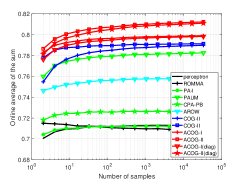
(a) a9a

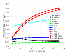
(b) covtype

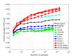
(c) german

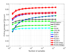
(d) ijcnn1

Figure 1: Evaluation of online “sum“ performance of the proposed algorithms on public datasets.

TABLE II: Evaluation of the Cost-Sensitive Classification Performance of ACOG and Other Algorithms

Algorithm	$``sum``$ on a9a				$``cost``$ on a9a
	Sum(%)	Sensitivity(%)	Specificity (%)	Time(s)	Cost($10^{2}$)	Sensitivity(%)	Specificity (%)	Time(s)
Perceptron	71.343 $\pm$ 0.215	56.406 $\pm$ 0.327	86.280 $\pm$ 0.102	0.196	50.951 $\pm$ 0.382	56.406 $\pm$ 0.327	86.280 $\pm$ 0.102	0.191
ROMMA	70.904 $\pm$ 0.239	57.918 $\pm$ 0.493	83.889 $\pm$ 0.262	0.225	50.184 $\pm$ 0.361	57.989 $\pm$ 0.346	83.863 $\pm$ 0.227	0.224
PA-I	71.274 $\pm$ 0.169	56.310 $\pm$ 0.277	86.237 $\pm$ 0.113	0.212	51.068 $\pm$ 0.311	56.310 $\pm$ 0.277	86.237 $\pm$ 0.113	0.212
PAUM	78.255 $\pm$ 0.155	70.868 $\pm$ 0.345	85.643 $\pm$ 0.116	0.192	35.976 $\pm$ 0.346	70.868 $\pm$ 0.345	85.643 $\pm$ 0.116	0.197
CPAPB	72.678 $\pm$ 0.209	62.818 $\pm$ 0.345	82.537 $\pm$ 0.145	0.254	42.517 $\pm$ 0.326	66.818 $\pm$ 0.285	79.503 $\pm$ 0.132	0.246
AROW	75.854 $\pm$ 0.188	58.858 $\pm$ 0.510	92.849 $\pm$ 0.153	5.591	45.931 $\pm$ 0.486	58.858 $\pm$ 0.510	92.849 $\pm$ 0.153	5.104
COG-I	78.978 $\pm$ 0.128	71.967 $\pm$ 0.264	85.990 $\pm$ 0.137	0.192	28.632 $\pm$ 0.263	79.390 $\pm$ 0.241	81.284 $\pm$ 0.107	0.190
COG-II	79.126 $\pm$ 0.103	81.038 $\pm$ 0.243	77.213 $\pm$ 0.168	0.201	25.527 $\pm$ 0.182	89.013 $\pm$ 0.171	62.398 $\pm$ 0.243	0.193
ACOG-I	79.903 $\pm$ 0.109	73.561 $\pm$ 0.347	86.244 $\pm$ 0.162	3.080	26.760 $\pm$ 0.291	81.129 $\pm$ 0.340	81.398 $\pm$ 0.219	2.837
ACOG-II	81.220 $\pm$ 0.108	85.269 $\pm$ 0.219	77.171 $\pm$ 0.134	3.344	20.307 $\pm$ 0.169	94.079 $\pm$ 0.136	62.107 $\pm$ 0.185	3.612
ACOG-Idiag	79.827 $\pm$ 0.094	73.361 $\pm$ 0.245	86.293 $\pm$ 0.103	0.202	26.917 $\pm$ 0.253	80.990 $\pm$ 0.282	81.369 $\pm$ 0.147	0.205
ACOG-IIdiag	81.098 $\pm$ 0.083	84.705 $\pm$ 0.227	77.491 $\pm$ 0.152	0.216	20.661 $\pm$ 0.110	93.352 $\pm$ 0.126	63.212 $\pm$ 0.238	0.213
Algorithm	$``sum``$ on covtype				$``cost``$ on covtype
	Sum(%)	Sensitivity(%)	Specificity (%)	Time(s)	Cost($10^{2}$)	Sensitivity(%)	Specificity (%)	Time(s)
Perceptron	52.609 $\pm$ 0.057	51.364 $\pm$ 0.058	53.854 $\pm$ 0.057	1.649	1377.464 $\pm$ 1.638	51.364 $\pm$ 0.058	53.854 $\pm$ 0.057	1.662
ROMMA	52.164 $\pm$ 0.674	50.819 $\pm$ 0.731	53.509 $\pm$ 0.647	2.233	1391.250 $\pm$ 19.560	50.860 $\pm$ 0.702	53.541 $\pm$ 0.614	2.295
PA-I	51.666 $\pm$ 0.056	50.324 $\pm$ 0.061	53.008 $\pm$ 0.063	1.869	1406.500 $\pm$ 1.675	50.324 $\pm$ 0.061	53.008 $\pm$ 0.063	1.913
PAUM	54.268 $\pm$ 0.059	52.588 $\pm$ 0.089	55.949 $\pm$ 0.066	1.693	1340.022 $\pm$ 2.311	52.588 $\pm$ 0.089	55.949 $\pm$ 0.066	1.709
CPAPB	51.667 $\pm$ 0.057	50.552 $\pm$ 0.063	52.781 $\pm$ 0.065	2.135	1194.433 $\pm$ 1.911	59.661 $\pm$ 0.070	44.275 $\pm$ 0.072	2.199
AROW	63.036 $\pm$ 0.033	60.158 $\pm$ 0.244	65.914 $\pm$ 0.213	22.640	687.696 $\pm$ 3.148	76.580 $\pm$ 0.137	69.579 $\pm$ 0.134	22.556
COG-I	54.268 $\pm$ 0.059	52.588 $\pm$ 0.089	55.949 $\pm$ 0.066	1.637	631.834 $\pm$ 1.721	84.036 $\pm$ 0.070	24.494 $\pm$ 0.062	1.710
COG-II	54.208 $\pm$ 0.051	54.038 $\pm$ 0.096	54.377 $\pm$ 0.055	1.643	426.122 $\pm$ 0.834	94.088 $\pm$ 0.031	7.501 $\pm$ 0.107	1.657
ACOG-I	68.077 $\pm$ 0.038	70.565 $\pm$ 0.073	65.588 $\pm$ 0.082	13.782	466.376 $\pm$ 1.190	90.693 $\pm$ 0.049	23.054 $\pm$ 0.038	18.988
ACOG-II	68.020 $\pm$ 0.030	71.265 $\pm$ 0.070	64.774 $\pm$ 0.068	13.528	305.056 $\pm$ 0.355	98.969 $\pm$ 0.021	6.365 $\pm$ 0.163	13.232
ACOG-Idiag	67.247 $\pm$ 0.060	69.183 $\pm$ 0.076	65.311 $\pm$ 0.082	1.824	469.701 $\pm$ 1.377	90.594 $\pm$ 0.090	22.782 $\pm$ 0.370	1.971
ACOG-IIdiag	67.225 $\pm$ 0.062	69.913 $\pm$ 0.096	64.537 $\pm$ 0.086	1.805	308.987 $\pm$ 7.944	98.739 $\pm$ 0.367	7.015 $\pm$ 0.507	1.828
Algorithm	$``sum``$ on german				$``cost``$ on german
	Sum(%)	Sensitivity(%)	Specificity (%)	Time(s)	Cost($10^{2}$)	Sensitivity(%)	Specificity (%)	Time(s)
Perceptron	53.760 $\pm$ 1.655	35.133 $\pm$ 2.343	72.386 $\pm$ 0.977	0.003	1.945 $\pm$ 0.070	35.133 $\pm$ 2.343	72.386 $\pm$ 0.977	0.003
ROMMA	57.625 $\pm$ 2.943	43.550 $\pm$ 4.496	71.700 $\pm$ 1.710	0.004	1.721 $\pm$ 0.128	43.650 $\pm$ 4.372	71.536 $\pm$ 1.932	0.004
PA-I	53.043 $\pm$ 1.902	34.000 $\pm$ 2.818	72.086 $\pm$ 1.128	0.003	1.977 $\pm$ 0.083	34.000 $\pm$ 2.818	72.086 $\pm$ 1.128	0.003
PAUM	54.145 $\pm$ 1.335	26.483 $\pm$ 3.633	81.807 $\pm$ 1.341	0.003	2.112 $\pm$ 0.091	26.483 $\pm$ 3.633	81.807 $\pm$ 1.341	0.003
CPAPB	53.185 $\pm$ 1.948	37.883 $\pm$ 2.925	68.486 $\pm$ 1.144	0.004	1.759 $\pm$ 0.082	44.317 $\pm$ 2.883	63.464 $\pm$ 1.287	0.004
AROW	59.948 $\pm$ 1.295	26.367 $\pm$ 3.893	93.529 $\pm$ 1.630	0.014	1.610 $\pm$ 0.082	43.867 $\pm$ 3.364	86.571 $\pm$ 1.543	0.016
COG-I	54.424 $\pm$ 1.474	36.083 $\pm$ 2.203	72.764 $\pm$ 0.807	0.003	1.770 $\pm$ 0.081	42.933 $\pm$ 3.010	67.200 $\pm$ 0.990	0.003
COG-II	54.952 $\pm$ 1.359	54.833 $\pm$ 1.318	55.071 $\pm$ 1.442	0.003	1.035 $\pm$ 0.033	81.067 $\pm$ 0.799	25.200 $\pm$ 1.983	0.003
ACOG-I	63.150 $\pm$ 1.025	49.050 $\pm$ 1.932	77.250 $\pm$ 1.489	0.008	1.232 $\pm$ 0.049	62.750 $\pm$ 2.017	67.671 $\pm$ 1.394	0.010
ACOG-II	62.511 $\pm$ 1.190	63.000 $\pm$ 2.052	62.021 $\pm$ 1.408	0.008	0.875 $\pm$ 0.044	86.883 $\pm$ 2.264	25.564 $\pm$ 4.099	0.011
ACOG-Idiag	61.765 $\pm$ 1.195	47.517 $\pm$ 2.610	76.014 $\pm$ 1.022	0.003	1.330 $\pm$ 0.064	58.967 $\pm$ 2.362	68.300 $\pm$ 0.901	0.003
ACOG-IIdiag	62.281 $\pm$ 1.428	62.883 $\pm$ 1.852	61.679 $\pm$ 1.576	0.003	0.912 $\pm$ 0.045	84.733 $\pm$ 0.876	28.629 $\pm$ 4.046	0.003
Algorithm	$``sum``$ on ijcnn1				$``cost``$ on ijcnn1
	Sum(%)	Sensitivity(%)	Specificity (%)	Time(s)	Cost($10^{2}$)	Sensitivity(%)	Specificity (%)	Time(s)
Perceptron	69.988 $\pm$ 0.252	45.926 $\pm$ 0.455	94.051 $\pm$ 0.050	0.112	26.303 $\pm$ 0.221	45.926 $\pm$ 0.455	94.051 $\pm$ 0.050	0.114
ROMMA	75.547 $\pm$ 0.229	57.689 $\pm$ 0.439	93.405 $\pm$ 0.111	0.124	21.467 $\pm$ 0.207	57.666 $\pm$ 0.459	93.404 $\pm$ 0.108	0.128
PA-I	69.980 $\pm$ 0.312	45.542 $\pm$ 0.579	94.418 $\pm$ 0.083	0.119	26.305 $\pm$ 0.274	45.542 $\pm$ 0.579	94.418 $\pm$ 0.083	0.124
PAUM	79.066 $\pm$ 0.275	64.377 $\pm$ 0.590	93.755 $\pm$ 0.092	0.112	18.378 $\pm$ 0.239	64.377 $\pm$ 0.590	93.755 $\pm$ 0.092	0.118
CPAPB	73.745 $\pm$ 0.209	57.328 $\pm$ 0.371	90.161 $\pm$ 0.091	0.155	23.096 $\pm$ 0.200	57.215 $\pm$ 0.407	90.233 $\pm$ 0.094	0.160
AROW	67.258 $\pm$ 0.460	36.208 $\pm$ 0.980	98.308 $\pm$ 0.074	0.450	28.626 $\pm$ 0.401	36.208 $\pm$ 0.980	98.308 $\pm$ 0.074	0.465
COG-I	79.066 $\pm$ 0.275	64.377 $\pm$ 0.590	93.755 $\pm$ 0.092	0.109	18.441 $\pm$ 0.236	64.171 $\pm$ 0.590	93.814 $\pm$ 0.096	0.116
COG-II	81.520 $\pm$ 0.232	81.940 $\pm$ 0.363	81.100 $\pm$ 0.182	0.112	16.398 $\pm$ 0.197	81.683 $\pm$ 0.311	81.394 $\pm$ 0.205	0.116
ACOG-I	82.375 $\pm$ 0.230	71.010 $\pm$ 0.607	93.740 $\pm$ 0.178	0.212	15.197 $\pm$ 0.123	71.996 $\pm$ 0.352	93.429 $\pm$ 0.102	0.218
ACOG-II	86.872 $\pm$ 0.174	88.924 $\pm$ 0.323	84.820 $\pm$ 0.218	0.288	12.279 $\pm$ 0.149	87.626 $\pm$ 0.293	84.770 $\pm$ 0.165	0.298
ACOG-Idiag	81.468 $\pm$ 0.225	69.007 $\pm$ 0.502	93.929 $\pm$ 0.092	0.114	15.681 $\pm$ 0.227	70.680 $\pm$ 0.624	93.631 $\pm$ 0.127	0.122
ACOG-IIdiag	86.929 $\pm$ 0.124	88.205 $\pm$ 0.266	85.652 $\pm$ 0.107	0.120	12.016 $\pm$ 0.111	87.164 $\pm$ 0.300	85.801 $\pm$ 0.138	0.122

4.2.2 Evaluation of Sum under Varying Weights

(a) a9a

(b) covtype

(c) german

(d) ijcnn1

Figure 2: Evaluation of weighted “sum“ performance under varying weights of sensitivity and specificity.

In this subsection, we would like to evaluate the $sum$ of proposed methods under different cost-sensitive weights. Fig. 2 shows the empirical results under different weights of $\alpha_{n}$ and $\alpha_{p}$. We find that our proposed algorithms consistently outperform all other algorithms under different values of weight on almost all datasets. This further validates the effectiveness of the proposed methods.

4.3 Evaluation with Cost Metrics

4.3.1 Evaluation of Weighted Cost Performance

Table 2 summaries the experimental performance of the ACOG_cost on 4 datasets in terms of $cost$ metrics, and Fig. 3 illustrates the development of online $cost$ performance at each iteration.

By evaluating the $cost$ performance in Fig. 3 and Table 2, our proposed methods achieve much lower misclassification $cost$ than other methods among all cases. For example, the overall $cost$ of ACOG is about less than half of $cost$ made by all regular first-order algorithms (i.e., perceptron, ROMMA, PA-I, PAUM and CPA_PB). This implies that introducing the second order information is beneficial to the decrease of misclassification $cost$.

In addition, by examining both $sensitivety$ and $specificity$ metrics, we observe that our proposed methods often achieve the best $sensitivity$ result on all datasets, and attain a relatively good $specificity$ among all cases.

Moreover, the diagonal ACOG_diag methods achieve higher $cost$ value than ACOG methods, but their running time are lower. This is similar with the situation based on $sum$ metric. Thus, the ACOG_diag methods can be regarded as a choice to balance the performance and efficiency.

(a) a9a

(b) covtype

(c) german

(d) ijcnn1

Figure 3: Evaluation of online “cost“ performance of the proposed algorithms on public datasets.

4.3.2 Evaluation of Cost under Varying Weights

In this subsection, we examine the $cost$ performance under different cost-sensitive weights $c_{n}$ and $c_{p}$ for our proposed algorithms. From the results in Fig. 4, we observe that the proposed algorithms outperform almost all other algorithms under different weights. And only on a few datasets, AROW can achieve similar performance with our proposed methods. These discoveries imply that our ACOG algorithms have a wide selection range of weight parameters for online classification tasks.

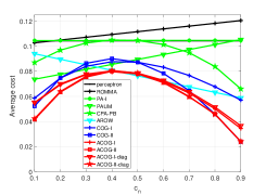
(a) a9a

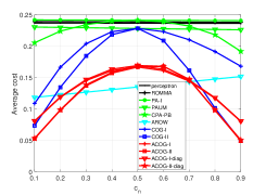
(b) covtype

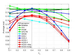
(c) german

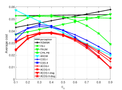
(d) ijcnn1

Figure 4: Evaluation of weighted “cost“ performance under varying weights for False Positives and False Negatives.

4.4 Evaluation of Algorithm properties

We have evaluated the performance of proposed algorithms in previous experiments, where promising results confirm their great superiority. Next, we are eager to examine their unique properties, including the influence of learning rate, regularized parameter, updating rule, online estimation and generalization ability. These examinations contribute to better understanding and applications of proposed methods. For simplicity, all experiments are based on $sum$ metric, and every experiment only considers one objective or variable, while all other variable settings are fixed and similar with before experiments.

4.4.1 Evaluation of Learning Rate

In this subsection, we evaluate the influence of learning rate. In detail, we examine the $sum$ performances of proposed methods with different learning rates $\eta$ from $[10^{-4},10^{-3},...,10^{3},10^{4}]$.

In Fig. 5, we find that ACOG algorithms would achieve relatively higher result, when we choose proper learning rate (i.e. relatively higher $\eta$ in general). This is easy to understand because the values of covariance matrix $\Sigma$ are normally small. Specifically, when a misclassification happened at time $t$, we update the predictive vector $\mu$ by $\mu_{t+1}=\mu_{t}+\eta\Sigma_{t+1}g_{t}$, where $g_{t}=\partial\ell_{t}(\mu_{t})$. Because the values of covariance matrix $\Sigma$ are normally small, the values of $\Sigma_{t+1}g_{t}$ thus are small. So if we want to obtain excellent performance, it would be better to choose properly higher learning rates as updating steps.

Moreover, we find the proposed methods with objective function $\ell^{II}(w;(x,y))$ can achieve relatively higher performance than the methods with $\ell^{I}(w;(x,y))$, which means that ACOG-II and ACOG-II_diag are more robust to different learning rate $\eta$ and consequently have a wider parameter choice space.

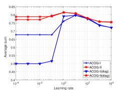
(a) a9a

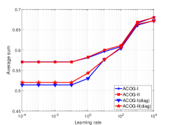
(b) covtype

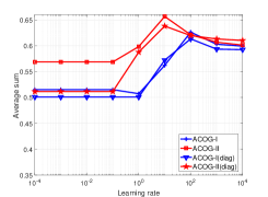
(c) german

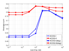
(d) ijcnn1

Figure 5: Performance under varying learning rates.

4.4.2 Evaluation of Regularized Parameter

Now, we aim to examine the influence of regularized parameters on our proposed algorithms.

When the learner makes a mistake, we update the covariance matrix $\Sigma$ by $\Sigma_{t+1}=\Sigma_{t}-\frac{\Sigma_{t}x_{t}x_{t}^{\top}\Sigma_{t}}{\gamma+x_{t}^{\top}\Sigma_{t}x_{t}}$ with default regularized parameter $\gamma$ as 1. However, the rationality of this setting is not verified. Thus, we examine the performance of our algorithms with different regularized parameters $\gamma$ from $[10^{-4},10^{-3},...,10^{3},10^{4}]$ for $sum$ metrics.

The results in Fig. 6 show that the optimal parameter normally is different according to datasets; while in most cases, the setting $\gamma=1$ can achieve the best or fairly good results. This discovery confirms the practical value of our algorithms with default settings.

(a) a9a

(b) covtype

(c) german

(d) ijcnn1

Figure 6: Performance under different regularized parameters.

4.4.3 Evaluation of Updating Rule

As mentioned in Section 2, the predictive vector $\mu$ is updated by $\mu_{t+1}=\mu_{t}+\eta\Sigma_{t+1}g_{t}$, which is different from AROW where the updating rule for $\mu$ relies on the old $\Sigma_{t}$. In this subsection, we would like to evaluate the difference between two updating rules based on $sum$ metrics for proposed methods, where the invariant versions (i.e., green line in Fig. 7) depending on old $\Sigma_{t}$.

From Fig. 7, we find that although the difference between two updating rules is not obvious, the performance of $\Sigma_{t+1}$ versions slightly exceed $\Sigma_{t}$ versions, which is consistent with our analysis in Section 2.

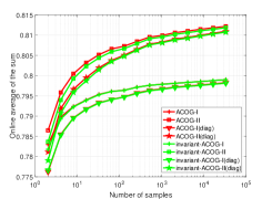
(a) a9a

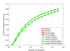
(b) covtype

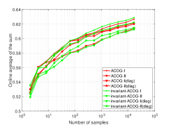
(c) german

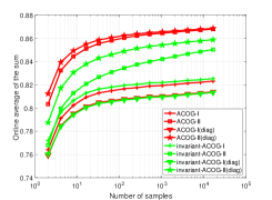
(d) ijcnn1

Figure 7: Evaluation of updating rules.

4.4.4 Evaluation of Online Estimation of $\frac{T_{n}}{T_{p}}$

In the remark of Algorithm 1, we analyzed the parameter $\rho=\frac{\eta_{p}T_{n}}{\eta_{n}T_{p}}$ for ACOG_sum algorithms, where the main question is that the value of $T_{p}$ and $T_{n}$ cannot be obtained in advance on real-world online learning.

Thus, we want to evaluate the influence of online estimation $\frac{T_{n}}{T_{p}}$ on $sum$ performance, compared with the original algorithms. We adopt the widely used laplace estimation here, which estimates $\frac{T_{n}}{T_{p}}$ by $\frac{t_{n}+1}{t_{p}+1}$, where $t_{p}$ and $t_{n}$ represent the number of positive samples and negative samples that have been seen, respectively.

Fig. 8 shows the performance of online estimation. We find that the online laplace estimation performs quite similar results with the original one. This discovery validates the practical value of the proposed ACOG_sum algorithms.

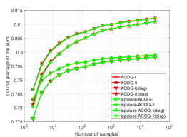
(a) a9a

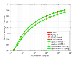
(b) covtype

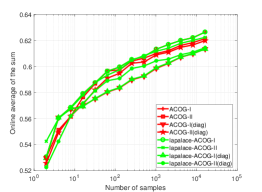
(c) german

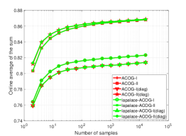
(d) ijcnn1

Figure 8: Evaluation of online estimation of $\frac{T_{n}}{T_{p}}$.

4.4.5 Evaluation of Generalization Ability

Then, we evaluate the generalization ability of proposed methods, which may exist problems when converting an online algorithm to a batch training approach. We use 5-fold cross-validation for better validation of the general performance.

Table 3 summary the consequences on $sum$ metrics, in which we discover that our proposed algorithms achieve the best among all algorithms on all datasets. This discovery indicates that our proposed methods have a strong generalized ability and can be regarded as a potentially useful tool to train large-scale cost-sensitive models.

TABLE III: Evaluation of generalization ability with $sum$

Algorithm	a9a	covtype	german	ijcnn1
Perceptron	68.649	51.553	53.737	70.045
ROMMA	72.467	67.059	58.614	76.818
PA-I	71.986	51.283	51.363	70.410
PAUM	79.323	53.354	52.126	82.012
CPAPB	73.668	51.279	52.768	73.942
AROW	75.961	64.928	54.575	67.642
COG-I	79.705	53.354	52.258	82.012
COG-II	78.559	68.897	50.784	82.849
ACOG-I	80.026	72.428	62.954	82.926
ACOG-II	81.630	72.632	60.928	87.730
ACOG-Idiag	80.118	71.051	64.389	82.334
ACOG-IIdiag	81.752	71.311	66.036	87.628

4.5 Performance and Efficiency of Sketched ACOG

In the previous experiments, the evaluations of the proposed ACOG algorithms have shown promising results. However, we can find the implementation of ACOG is time consuming when facing high-dimensional datasets, because of the updating step for covariance matrix. As a result, it is difficult for engineers to address the real-world tasks with quite large-scale datasets.

A simple solution to this question is to implement the diagonal version of ACOG, and then enjoy linear time complexity. However, the gain of diagonal ACOG is at the cost of lower performance, because it abandons the correlation information between sample dimensions, which is quite important and indispensable for datasets with strong inner-correlation. Thus, for better trade off between performance and time efficiency, we propose the Sketched ACOG (named SACOG) and its sparse version (named SSACOG).

In this section, we first evaluate our sketched algorithms with several baseline algorithms: (1) “COG-I“ and “COG-II“; (2) “ACOG-I“ and “ACOG-II“; (3) “ACOG-I_diag“ and “ACOG-II_diag“, where we adopt 4 relatively high-dimensional datasets from LIBSVM, which are higher than 45 dimensions as list in Table 4. After that, we examine the performance difference between SACOG and SSACOG.

For simplicity, we focus on the case that the sketch size $m$ is fixed as 5 for all sketched algorithms, although our methods can be easily generalized by setting different sketch sizes like [44]. Moreover, the learning rate was selected from $[10^{-5},10^{-4},...,10^{5}]$, where other implementation details are similar with [44]. In addition, all experimental settings for other algorithms are same as previous experiments.

TABLE IV: Datasets for Evaluation of Sketched Algorithm

Dataset	#Examples	#Features	#Pos:#Neg
mushrooms	8124	112	1:1.07
protein	17766	357	1:1.7
usps	7291	256	1:5.11
Sensorless	58509	48	1:10

4.5.1 Evaluation of Weighted Sum Performance

In this subsection, we would like to examine the performance and efficiency of our sketched algorithms, where we adopt the sparse version (SSACOG) rather than the original SACOG, which is more appropriate for real-world datasets.

The results are summarized in Fig. 9, Fig. 10 and Table 5 based on two metrics, from which we find that the proposed SSACOG is much faster than ACOG algorithms, while the performance of sketched algorithms is not affected too much and sometimes even better. In addition, the degree of efficiency optimization by sketching technique goes up along with the increase of data dimensions, which is consistent with the common sense.

Note that although the running time of SSACOG is slower than ACOG_diag, it enjoys higher performance due to the advantage of sufficient second-order information. This confirms the superiority of ACOG with sketching technique.

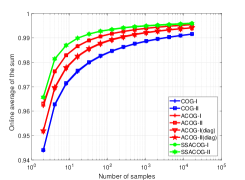
(a) mushrooms

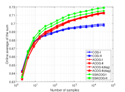
(b) protein

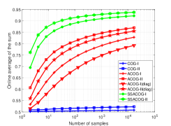
(c) Sensorless

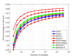
(d) usps

Figure 9: Weighted “sum“ performance of SACOG.

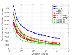
(a) mushrooms

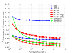
(b) protein

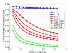
(c) Sensorless

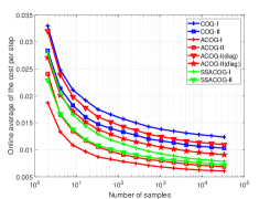
(d) usps

Figure 10: Weighted “cost“ performance of SACOG.

TABLE V: Evaluation of the Cost-Sensitive Classification Performance of SSACOG

Algorithm	$``sum``$ on mushrooms				$``cost``$ on mushrooms
	Sum(%)	Sensitivity(%)	Specificity (%)	Time(s)	Cost	Sensitivity(%)	Specificity (%)	Time(s)
COG-I	99.205 $\pm$ 0.047	99.455 $\pm$ 0.075	98.956 $\pm$ 0.095	0.019	15.760 $\pm$ 2.496	99.823 $\pm$ 0.070	97.688 $\pm$ 0.091	0.020
COG-II	99.211 $\pm$ 0.057	99.420 $\pm$ 0.094	99.003 $\pm$ 0.097	0.019	39.180 $\pm$ 2.283	99.538 $\pm$ 0.055	94.465 $\pm$ 0.275	0.019
ACOG-I	99.580 $\pm$ 0.027	99.810 $\pm$ 0.070	99.350 $\pm$ 0.076	0.043	18.735 $\pm$ 1.062	99.939 $\pm$ 0.051	95.802 $\pm$ 0.443	0.085
ACOG-II	99.572 $\pm$ 0.033	99.794 $\pm$ 0.080	99.349 $\pm$ 0.075	0.045	16.770 $\pm$ 1.546	99.932 $\pm$ 0.035	96.373 $\pm$ 0.412	0.054
ACOG-Idiag	99.447 $\pm$ 0.052	99.652 $\pm$ 0.077	99.243 $\pm$ 0.087	0.019	17.520 $\pm$ 1.588	99.933 $\pm$ 0.045	98.119 $\pm$ 0.060	0.020
ACOG-IIdiag	99.457 $\pm$ 0.052	99.652 $\pm$ 0.086	99.262 $\pm$ 0.117	0.019	21.185 $\pm$ 1.431	99.792 $\pm$ 0.037	96.601 $\pm$ 0.167	0.019
SSACOG-I	99.628 $\pm$ 0.052	99.798 $\pm$ 0.066	99.459 $\pm$ 0.102	0.038	15.880 $\pm$ 1.677	99.930 $\pm$ 0.043	96.623 $\pm$ 0.303	0.041
SSACOG-II	99.606 $\pm$ 0.050	99.805 $\pm$ 0.062	99.408 $\pm$ 0.093	0.038	15.560 $\pm$ 3.870	99.869 $\pm$ 0.040	97.291 $\pm$ 1.063	0.034
Algorithm	$``sum``$ on protein				$``cost``$ on protein
	Sum(%)	Sensitivity(%)	Specificity (%)	Time(s)	Cost	Sensitivity(%)	Specificity (%)	Time(s)
COG-I	69.935 $\pm$ 0.213	68.114 $\pm$ 0.343	71.757 $\pm$ 0.322	0.127	2156.980 $\pm$ 35.558	75.944 $\pm$ 0.463	60.071 $\pm$ 0.270	0.151
COG-II	69.764 $\pm$ 0.230	70.005 $\pm$ 0.392	69.523 $\pm$ 0.415	0.129	1375.740 $\pm$ 12.402	90.618 $\pm$ 0.106	28.559 $\pm$ 0.607	0.152
ACOG-I	71.340 $\pm$ 0.214	69.794 $\pm$ 0.427	72.886 $\pm$ 0.385	14.603	1406.660 $\pm$ 28.314	87.072 $\pm$ 0.428	52.671 $\pm$ 0.576	16.922
ACOG-II	71.265 $\pm$ 0.235	71.678 $\pm$ 0.398	70.852 $\pm$ 0.501	14.446	1110.075 $\pm$ 12.274	94.972 $\pm$ 0.172	22.753 $\pm$ 0.853	13.601
ACOG-Idiag	71.305 $\pm$ 0.126	69.825 $\pm$ 0.346	72.785 $\pm$ 0.257	0.161	1441.505 $\pm$ 19.496	86.500 $\pm$ 0.269	53.441 $\pm$ 0.394	0.171
ACOG-IIdiag	71.233 $\pm$ 0.150	71.530 $\pm$ 0.365	70.935 $\pm$ 0.298	0.158	1198.455 $\pm$ 11.459	92.585 $\pm$ 0.143	31.925 $\pm$ 0.685	0.166
SSACOG-I	71.532 $\pm$ 0.198	66.861 $\pm$ 0.530	76.203 $\pm$ 0.485	0.355	1227.345 $\pm$ 16.904	90.608 $\pm$ 0.225	44.148 $\pm$ 0.342	0.393
SSACOG-II	71.323 $\pm$ 0.132	71.725 $\pm$ 0.305	72.075 $\pm$ 0.403	0.352	1144.680 $\pm$ 13.087	94.053 $\pm$ 0.144	26.224 $\pm$ 0.661	0.348
Algorithm	$``sum``$ on Sensorless				$``cost``$ on Sensorless
	Sum(%)	Sensitivity(%)	Specificity (%)	Time(s)	Cost	Sensitivity(%)	Specificity (%)	Time(s)
COG-I	50.888 $\pm$ 0.227	9.637 $\pm$ 0.473	92.139 $\pm$ 0.076	0.166	4741.190 $\pm$ 21.159	11.155 $\pm$ 0.403	90.823 $\pm$ 0.038	0.154
COG-II	52.374 $\pm$ 0.422	52.717 $\pm$ 0.464	52.032 $\pm$ 0.387	0.167	4801.600 $\pm$ 38.579	50.168 $\pm$ 0.415	54.576 $\pm$ 0.354	0.149
ACOG-I	83.468 $\pm$ 0.308	72.935 $\pm$ 0.620	94.001 $\pm$ 0.068	0.503	1622.600 $\pm$ 32.312	72.563 $\pm$ 0.709	94.188 $\pm$ 0.078	0.480
ACOG-II	87.398 $\pm$ 0.186	88.088 $\pm$ 0.284	86.708 $\pm$ 0.178	0.486	1283.350 $\pm$ 16.768	87.247 $\pm$ 0.264	87.350 $\pm$ 0.131	0.455
ACOG-Idiag	80.044 $\pm$ 0.314	66.427 $\pm$ 0.627	93.661 $\pm$ 0.051	0.169	1956.200 $\pm$ 33.729	65.995 $\pm$ 0.668	93.827 $\pm$ 0.071	0.157
ACOG-IIdiag	85.968 $\pm$ 0.124	86.608 $\pm$ 0.178	85.328 $\pm$ 0.118	0.173	1422.950 $\pm$ 16.836	85.783 $\pm$ 0.227	86.043 $\pm$ 0.131	0.153
SSACOG-I	92.432 $\pm$ 0.213	89.818 $\pm$ 0.442	95.047 $\pm$ 0.047	0.322	753.695 $\pm$ 21.185	89.482 $\pm$ 0.476	95.296 $\pm$ 0.066	0.285
SSACOG-II	93.913 $\pm$ 0.129	94.487 $\pm$ 0.181	93.339 $\pm$ 0.123	0.296	615.625 $\pm$ 12.280	94.166 $\pm$ 0.194	93.676 $\pm$ 0.096	0.264
Algorithm	$``sum``$ on usps				$``cost``$ on usps
	Sum(%)	Sensitivity(%)	Specificity (%)	Time(s)	Cost	Sensitivity(%)	Specificity (%)	Time(s)
COG-I	96.820 $\pm$ 0.165	96.361 $\pm$ 0.345	97.279 $\pm$ 0.116	0.039	90.165 $\pm$ 3.851	92.642 $\pm$ 0.344	98.179 $\pm$ 0.060	0.031
COG-II	96.576 $\pm$ 0.139	96.516 $\pm$ 0.226	96.637 $\pm$ 0.193	0.038	75.135 $\pm$ 4.338	96.570 $\pm$ 0.215	93.722 $\pm$ 0.342	0.030
ACOG-I	98.073 $\pm$ 0.115	97.822 $\pm$ 0.242	98.323 $\pm$ 0.095	0.271	44.365 $\pm$ 3.448	96.671 $\pm$ 0.321	98.591 $\pm$ 0.070	0.151
ACOG-II	97.633 $\pm$ 0.148	97.998 $\pm$ 0.230	97.268 $\pm$ 0.176	0.239	50.100 $\pm$ 4.321	98.241 $\pm$ 0.172	94.883 $\pm$ 0.488	0.252
ACOG-Idiag	96.886 $\pm$ 0.226	95.641 $\pm$ 0.435	98.131 $\pm$ 0.076	0.039	79.850 $\pm$ 4.773	93.526 $\pm$ 0.423	98.314 $\pm$ 0.080	0.031
ACOG-IIdiag	96.305 $\pm$ 0.182	96.369 $\pm$ 0.228	96.240 $\pm$ 0.182	0.040	66.300 $\pm$ 3.242	96.993 $\pm$ 0.149	94.425 $\pm$ 0.295	0.030
SSACOG-I	97.091 $\pm$ 0.197	96.817 $\pm$ 0.323	97.365 $\pm$ 0.125	0.077	57.055 $\pm$ 4.251	95.657 $\pm$ 0.384	98.296 $\pm$ 0.076	0.054
SSACOG-II	97.048 $\pm$ 0.163	97.010 $\pm$ 0.237	97.085 $\pm$ 0.190	0.074	52.420 $\pm$ 4.009	97.647 $\pm$ 0.192	95.550 $\pm$ 0.360	0.054

TABLE VI: Evaluation between SACOG and Sparse SACOG

Algorithm	$``sum``$ on mushrooms		$``cost``$ on mushrooms		$``sum``$ on protein		$``cost``$ on protein
	Sum(%)	Time(s)	Cost($10^{2}$)	Time(s)	Sum(%)	Time(s)	Cost($10^{2}$)	Time(s)
SACOG-I	99.620 $\pm$ 0.043	0.072	16.020 $\pm$ 1.796	0.096	71.544 $\pm$ 0.197	3.769	1226.890 $\pm$ 17.094	3.302
SACOG-II	99.598 $\pm$ 0.040	0.074	13.790 $\pm$ 1.852	0.035	71.907 $\pm$ 0.180	3.705	1147.775 $\pm$ 14.364	2.373
SSACOG-I	99.628 $\pm$ 0.052	0.038	15.880 $\pm$ 1.677	0.039	71.532 $\pm$ 0.198	0.287	1227.345 $\pm$ 16.904	0.272
SSACOG-II	99.606 $\pm$ 0.050	0.038	15.560 $\pm$ 3.870	0.033	71.900 $\pm$ 0.204	0.285	1144.680 $\pm$ 13.087	0.239
Algorithm	$``sum``$ on Sensorless		$``cost``$ on Sensorless		$``sum``$ on usps		$``cost``$ on usps
	Sum(%)	Time(s)	Cost($10^{2}$)	Time(s)	Sum(%)	Time(s)	Cost($10^{2}$)	Time(s)
SACOG-I	92.432 $\pm$ 0.213	0.232	753.695 $\pm$ 21.185	0.235	97.146 $\pm$ 0.149	0.135	55.970 $\pm$ 3.053	0.078
SACOG-II	93.913 $\pm$ 0.129	0.193	615.625 $\pm$ 12.280	0.194	97.071 $\pm$ 0.169	0.091	53.155 $\pm$ 4.815	0.090
SSACOG-I	92.432 $\pm$ 0.213	0.239	753.695 $\pm$ 21.185	0.225	97.091 $\pm$ 0.197	0.057	57.055 $\pm$ 4.251	0.052
SSACOG-II	93.913 $\pm$ 0.129	0.214	615.625 $\pm$ 12.280	0.204	97.048 $\pm$ 0.163	0.054	52.420 $\pm$ 4.009	0.053

4.5.2 Efficiency Comparison between Sketched ACOG and Sparse Sketched ACOG

Then, We would like to compare the performance and running time between SACOG and its sparse version SSACOG. The experimental results based on both metrics are summarized in Table 6.

From results, we find that the running time of SSACOG is lower than SACOG. It is consistent with the time complexity analysis of two algorithms in Section 3. For better understanding, we simply give a analysis. Given sketch size $m=5$, the time complexity for SACOG is $O(25d)$ according to the analysis of Section 3, while the time complexity for SSACOG is $O(125+5s)$. One can accelerate the time complexity to $O(5d)$ for SACOG and $O(25+5s)$ for SSACOG by only updating the sketch every $m$ round.

Thus, the time complexity for SACOG is linear in the data dimensionality $d$, and running time for SSACOG is linear in the data non-sparse degree $s$. Then, it is easy to understand the SSACOG would be much faster than SACOG, when the data dimensionality $d$ is high and the data sparsity is strong $s\ll d$.

5 Application to Online Anomaly Detection

The proposed adaptive regularized cost-sensitive online classification algorithms can be potentially applied to solve a wide range of real-world applications in data mining. To verify their practical application value, we apply them to tackle several online anomaly detection tasks in this section.

5.1 Application Domains and Testbeds

Below, we first exhibit the related domains of anomaly detection problems:

$\bullet$ Finance: The credit card approval problem enjoys a huge demand in financial domains, where our task is to discriminate the credit-worthy customers for the Australian dataset from an Australian credit company.

$\bullet$ Nuclear: We apply our algorithms to the Magic04 dataset with 19020 samples to simulate registration of high gamma particles. The dataset was collected by a ground-based atmospheric Cherenkov gamma telescope. In detail, the “gamma signal“ samples are considered as the normal class, while the hadron ones are treated as outliers.

$\bullet$ Bioinformatics: We address bioinformatics anomaly detection problems with DNA dataset to recognize the boundaries between exons and introns from a given DNA sequence, where exon/intron boundaries are defined as anomalies and others are treated as normal.

$\bullet$ Medical Imaging: We apply our approaches to address the medical image anomaly detection problem with the KDDCUP08 breast cancer dataset. The main goal is to detect the breast cancer from X-ray images, where “benign“ is assigned as normal and “malignant“ is abnormal.

To better understand, we summary the detailed information for each dataset in Table 7.

TABLE VII: Datasets for Online Anomaly Detection

Dataset	#Examples	#Features	#Pos:#Neg
Australian	690	14	1:1.25
Magic04	19020	10	1:1.8
DNA	2000	180	1:3.31
KDDCUP08	102294	117	1:163.19

5.2 Empirical Evaluation Results

In this subsection, our algorithms are applied to address real-world anomaly detection tasks with 4 datasets from different domains, where we use the balanced accuracy metric to avoid inflated performance evaluations on imbalanced datasets. In addition, we apply our sparse sketched ACOG algorithms (SSACOG) only for two high-dimensional datasets (i.e., DNA and KDDCUP08), because for low-dimensional tasks, the proposed ACOG algorithms are fast enough. Furthermore, all implementation settings are same as Section 4.

Table 8 exhibits the experimental results, from which we can draw several observations. First of all, two cost-sensitive methods (PAUM and CPA_PB) outperform their regular methods (Perceptron and PA-I) among all datasets. This confirms the superiority of cost-sensitiveness for online learning. Second, COG algorithms outperform all regular first-order algorithms (i.e., first 5 baselines) on almost all datasets, which demonstrates the effectiveness of direct cost-sensitive optimization in online learning.

Moreover, ACOG algorithms and AROW algorithm outperform all other algorithms, where ACOG is the updated version of COG with adaptive regularization using second order information. This infers the online classification that introduces the second-order inner-correlation information can enjoy a huge performance improvement. Furthermore, the performance of ACOG exceeds all other algorithms, which demonstrates the effectiveness of cost-sensitive online optimization using the second order information.

By the way, although the speed of SSACOG is slightly slower than ACOG_diag, its performance is relatively better. On the other hand, SSACOG is much faster than ACOG with slight performance loss. This implies that the sketching version of ACOG is a good choice to balance the performance and efficiency for handling high-dimensional real-world tasks. Furthermore, if someone only wants to pursue the efficiency, they can regard ACOG_diag as a choice.

In conclusion, all promising results confirm the superiority of our proposed algorithms for real-world online anomaly detection problems, where datasets are normally high-dimensional and highly class-imbalanced.

6 Conclusion

In this paper, to remedy the weakness of first-order cost-sensitive online learning algorithms, we propose to introduce second-order information into cost-sensitive online classification framework based on adaptive regularization. As a result, a family of second-order cost-sensitive online classification algorithms is proposed, with favourable regret bound and impressive properties.

Moreover, to overcome the time-consuming problem of our second-order algorithms, we further study the sketching method in cost-sensitive online classification framework, and then propose sketched cost-sensitive online classification algorithms, which can be developed as a sparse cost-sensitive online learning approach, with better trade off between the performance and efficiency.

Then for examination of the performance and efficiency, we empirically evaluate our proposed algorithms on many public real-world datasets in extensive experiments. Promising results not only prove the new proposed algorithms successfully overcome the limitation of first-order algorithms, but also confirm their effectiveness and efficiency in solving real-world cost-sensitive online classification problems.

Future works include: (i) further exploration about the in-depth theory of cost-sensitive online learning; (ii) further study about the sparse computation methods in cost-sensitive online classification problems.

TABLE VIII: Evaluation for online anomaly detection

Algorithm	$``sum``$ on Australian		$``sum``$ on Magic04
	Sum(%)	Time(s)	Sum(%)	Time(s)
Perceptron	57.863 $\pm$ 1.327	0.002	59.154 $\pm$ 0.408	0.030
ROMMA	58.732 $\pm$ 3.462	0.002	64.025 $\pm$ 3.277	0.042
PA-I	57.103 $\pm$ 1.595	0.002	58.029 $\pm$ 0.312	0.036
PAUM	62.362 $\pm$ 0.941	0.002	64.671 $\pm$ 0.204	0.030
CPAPB	57.110 $\pm$ 1.599	0.003	58.448 $\pm$ 0.360	0.043
AROW	67.174 $\pm$ 0.749	0.008	70.896 $\pm$ 0.190	0.154
COG-I	65.972 $\pm$ 0.879	0.002	65.913 $\pm$ 0.189	0.030
COG-II	67.213 $\pm$ 0.787	0.002	69.815 $\pm$ 0.183	0.030
ACOG-I	68.808 $\pm$ 0.894	0.005	72.935 $\pm$ 0.186	0.088
ACOG-II	69.228 $\pm$ 0.733	0.005	68.345 $\pm$ 1.822	0.092
ACOG-Idiag	68.464 $\pm$ 0.936	0.002	73.268 $\pm$ 0.158	0.033
ACOG-IIdiag	68.510 $\pm$ 0.917	0.002	73.035 $\pm$ 0.187	0.033
Algorithm	$``sum``$ on DNA		$``sum``$ on KDDCUP08
	Sum(%)	Time(s)	Sum(%)	Time(s)
Perceptron	84.759 $\pm$ 0.575	0.006	54.018 $\pm$ 1.056	0.376
ROMMA	85.782 $\pm$ 0.553	0.006	54.342 $\pm$ 1.581	0.507
PA-I	87.832 $\pm$ 0.833	0.005	54.053 $\pm$ 0.865	0.414
PAUM	88.560 $\pm$ 0.737	0.005	55.161 $\pm$ 0.424	0.386
CPAPB	89.401 $\pm$ 0.645	0.007	57.318 $\pm$ 0.629	0.458
AROW	89.183 $\pm$ 0.405	0.269	50.611 $\pm$ 0.422	12.554
COG-I	87.886 $\pm$ 0.812	0.006	54.094 $\pm$ 1.047	0.355
COG-II	87.395 $\pm$ 0.530	0.005	69.312 $\pm$ 0.475	0.359
ACOG-I	91.490 $\pm$ 0.416	0.104	55.088 $\pm$ 0.936	4.531
ACOG-II	90.872 $\pm$ 0.677	0.234	71.920 $\pm$ 2.016	5.803
ACOG-Idiag	89.498 $\pm$ 0.633	0.006	55.293 $\pm$ 0.852	0.384
ACOG-IIdiag	88.433 $\pm$ 0.490	0.006	71.661 $\pm$ 1.334	0.397
SSACOG-I	89.975 $\pm$ 0.516	0.016	55.711 $\pm$ 0.812	0.810
SSACOG-II	90.444 $\pm$ 0.471	0.023	70.947 $\pm$ 1.179	0.842

7 Acknowledgement

This research is partly supported by the National Research Foundation, Prime Minister s Office, Singapore under its International Research Centres in Singapore Funding Initiative, and partly supported by National Natural Science Foundation of China (NSFC) under Grant 61602185, Fundamental Research Funds for the Central Universities under Grant D2172480.

Peilin Zhao is currently a researcher with SCUT, China. His research interests are Large-Scale Machine Learning and its applications to Big Data Analytics. Previously, he has worked at Ant Financial, Institute for Infocomm Research (I2R), Rutgers University. He received his PHD degree from Nanyang Technological University and his bachelor degree from Zhejiang University. In his research areas, he has published over 70 papers in top venues, including JMLR, AIJ, ICML, NIPS, KDD, etc. He has been invited as a PC member or reviewer for many international conferences and journals in his area.

Yifan Zhang received the BE degree in electronic commerce from the Southwest University, China, in 2017. He is working toward the ME degree in the School of Software Engineering, South China University of Technology, China. His research interests include Machine Learning, Reinforcement Learning and their applications in Big Data Analytics.

Min Wu is a research scientist in Data Analytics Department, Institute for Infocomm Research. He received Ph.D degree from Nanyang Technological University, Singapore, in 2011, and received B.S. degree in Computer Science from University of Science and Technology of China, 2006. His research interests include Graph Mining from Large-Scale Networks, Learning from Heterogeneous Data Sources, Ensemble Learning, and Bioinformatics.

Steven C. H. Hoi is an Associate Professor in Singapore Management University (SMU), Singapore. Prior to joining SMU, he was a tenured Associate Professor at Nanyang Technological University (NTU), Singapore. He received his Bachelor degree from Tsinghua University, and his Master and Ph.D degrees from the Chinese University of Hong Kong. His research interests include large-scale machine learning with application to a wide range of real-world applications. He has published over 150 papers in premier conferences and journals, and served as an organizer, area chair, senior PC, TPC member, editors, and referee for many top conferences and premier journals. He is the recipient of the Lee Kong Chian Fellowship Award due to his research excellence.

Mingkui Tan received the PhD degree in computer science from Nanyang Technological University, Singapore, in 2014. He is a professor in the School of Software Engineering, South China University of Technology. After that, he worked as a senior research associate in the School of Computer Science, University of Adelaide, Australia. His research interests include compressive sensing, big data learning, and large-scale optimization.

Junzhou Huang is an Associate Professor in the Computer Science and Engineering department at the University of Texas at Arlington. He received the B.E. degree from Huazhong University of Science and Technology, China, the M.S. degree from Chinese Academy of Sciences, China, and the Ph.D. degree in Rutgers university. His major research interests include machine learning, computer vision and imaging informatics. He was selected as one of the 10 emerging leaders in multimedia and signal processing by the IBM T.J. Watson Research Center in 2010. He received the NSF CAREER Award in 2016.

Supplementary Materials
Adaptive Cost-Sensitive Online Classification Peilin Zhao, Yifan Zhang, Min Wu, Steven C. H. Hoi, Mingkui Tan, and Junzhou Huang P. Zhao, Y. Zhang and M. Tan are with the South China University of Technology, China. E-mail: peilinzhao@hotmail.com; sezyifan@mail.scut.edu.cn; mingkuitan@scut.edu.cn. M. Wu is with the Institute for Infocomm Research, Singapore. E-mail: wumin@i2r.a-star.edu.sg. S. C. Hoi is with the Singapore Management University, Singapore. E-mail: chhoi@smu.edu.sg. J. Huang is with Tencent AI Lab, China. Email: joehhuang@tencent.com. Y. Zhang is the co-first author; M. Tan is the corresponding author.

Appendix A Proofs of Theorems

This section presents the proofs for all the theorems.

A.1 Proof of Theorem 1

Proof.  It is easy to verify $\mu_{t+1}={\rm arg\min}_{\mu}h_{t}(\mu)$, where $h_{t}(\mu)=\frac{1}{2}||\mu_{t}-\mu||_{\Sigma^{-1}_{t+1}}^{2}+\eta g_{t}^{\top}\mu$. Since $h_{t}$ is convex and continuous, through proof by contradiction, one can easily have:

$$\partial h_{t}(\mu_{t+1})^{\top}(\mu-\mu_{t+1})$$

$$= [(\mu_{t+1}-\mu_{t})^{\top}\Sigma_{t+1}^{-1}+\eta g_{t}^{\top}](\mu-\mu_{t+1})\geq 0,\forall\mu.$$

Re-arrange the inequality will give:

$$(\eta g_{t})^{\top}(\mu_{t+1}-\mu)\leq (\mu_{t+1}-\mu_{t})^{\top}\Sigma_{T+1}^{-1}(\mu-\mu_{t+1})$$

$$= \frac{1}{2}[||\mu_{t}-\mu||_{\Sigma^{-1}_{t+1}}^{2}-||\mu_{t+1}-\mu||_{\Sigma^{-1}_{t+1}}^{2}$$

$$\ -||\mu_{t}-\mu_{t+1}||_{\Sigma^{-1}_{t+1}}^{2}].$$

Then, since $\ell_{t}(\mu)$ is convex function, we have:

$$g_{t}^{\top}(\mu_{t+1}-\mu)= g_{t}^{\top}(\mu_{t+1}-\mu+\mu_{t}-\mu_{t})$$

$$= g_{t}^{\top}(\mu_{t}-\mu)+g_{t}^{\top}(\mu_{t+1}-\mu_{t})$$

$$\geq \ell_{t}(\mu_{t})-\ell_{t}(\mu)+g_{t}^{\top}(\mu_{t+1}-\mu_{t}).$$

Next, combining the above two inequalities gives the following key inequality:

$$\ell_{t}(\mu_{t})-\ell_{t}(\mu)\leq \frac{1}{2\eta}[||\mu_{t}-\mu||_{\Sigma^{-1}_{t+1}}^{2}-||\mu_{t+1}-\mu||_{\Sigma^{-1}_{t+1}}^{2}$$

$$\ -||\mu_{t}-\mu_{t+1}||_{\Sigma^{-1}_{t+1}}^{2}]-g_{t}^{\top}(\mu_{t+1}-\mu_{t}).$$

Summing the inequality above over $t=1,2,...T$, gives:

$$\sum_{t=1}^{T}[\ell_{t}(\mu_{t})-\ell_{t}(\mu)]$$

$$\leq\frac{1}{2\eta}\sum_{t=1}^{T}[||\mu_{t}-\mu||_{\Sigma^{-1}_{t+1}}^{2}-||\mu_{t+1}-\mu||_{\Sigma^{-1}_{t+1}}^{2}]$$

$$\ -\frac{1}{2\eta}\sum_{t=1}^{T}||\mu_{t}-\mu_{t+1}||_{\Sigma^{-1}_{t+1}}^{2}]-\sum_{t=1}^{T}g_{t}^{\top}(\mu_{t+1}-\mu_{t}).$$ (19)

Now, we bound the right side of inequality by dividing two parts. For the first term, we can bound as:

$$\sum_{t=1}^{T}[||\mu_{t}-\mu||_{\Sigma^{-1}_{t+1}}^{2}-||\mu_{t+1}-\mu||_{\Sigma^{-1}_{t+1}}^{2}]$$

$$\leq||\mu_{1}-\mu||_{\Sigma^{-1}_{2}}^{2}+\sum_{t=2}^{T}[||\mu_{t}-\mu||_{\Sigma^{-1}_{t+1}}^{2}-||\mu_{t}-\mu||_{\Sigma^{-1}_{t}}^{2}]$$

$$=||\mu_{1}-\mu||_{\Sigma^{-1}_{2}}^{2}+\sum_{t=2}^{T}[||\mu_{t}-\mu||_{(\Sigma^{-1}_{t+1}-\Sigma^{-1}_{t})}^{2}]$$

$$\leq||\mu_{1}\small{-}\mu||^{2}\lambda_{max}(\Sigma_{2}^{-1})+\sum_{t=2}^{T}||\mu_{t}\small{-}\mu||^{2}\lambda_{max}(\Sigma^{-1}_{t+1}\small{-}\Sigma^{-1}_{t})$$

$$\leq||\mu_{1}-\mu||^{2}{\rm Tr}(\Sigma_{2}^{-1})+\sum_{t=2}^{T}||\mu_{t}-\mu||^{2}{\rm Tr}(\Sigma^{-1}_{t+1}-\Sigma^{-1}_{t})$$

$$\leq\max_{t\leq T}||\mu_{t}\small{-}\mu||^{2}{\rm Tr}(\Sigma_{2}^{-1})\small{+}\sum_{t=2}^{T}\max_{t\leq T}||\mu_{t}\small{-}\mu||^{2}{\rm Tr}(\Sigma^{-1}_{t+1}\small{-}\Sigma^{-1}_{t})$$

$$=\max_{t\leq T}||\mu_{t}\small{-}\mu||^{2}{\rm Tr}(\Sigma_{T+1}^{-1}),$$ (20)

where $\lambda_{max}(\Sigma)$ is the largest eigenvalue of $\Sigma$. Then, we bound the remain terms. From the updating rule of $\mu$, we have:

$$(\mu_{t+1}-\mu_{t})^{\top}\Sigma_{t+1}^{-1}+\eta g_{t}^{\top}=0,$$

so that:

$$||\mu_{t}-\mu_{t+1}||_{\Sigma^{-1}_{t+1}}^{2}$$

$$=(\mu_{t+1}-\mu_{t})^{\top}\Sigma_{t+1}^{-1}\Sigma_{t+1}\Sigma_{t+1}^{-1}(\mu_{t+1}-\mu_{t})$$

$$=\eta^{2}g_{t}^{\top}\Sigma_{t+1}g_{t},$$

and

$$g_{t}^{\top}(\mu_{t+1}-\mu_{t})=-\eta g_{t}^{\top}\Sigma_{t+1}g_{t}.$$ (21)

Combining the two inequalities causes in:

$$-\frac{1}{2\eta}\sum_{t=1}^{T}||\mu_{t}-\mu_{t+1}||_{\Sigma^{-1}_{t+1}}^{2}-\sum_{t=1}^{T}g_{t}^{\top}(\mu_{t+1}-\mu_{t})$$

$$=\sum_{t=1}^{T}\eta g_{t}^{\top}\Sigma_{t+1}g_{t}-\sum_{t=1}^{T}\frac{\eta}{2}g_{t}^{\top}\Sigma_{t+1}g_{t}$$

$$=\frac{\eta}{2}\sum_{t=1}^{T}g_{t}^{\top}\Sigma_{t+1}g_{t}.$$ (22)

As we know, we have $g_{t}=L_{t}y_{t}x_{t}$ for ACOG-I, where $L_{t}=\mathbb{I}_{(\ell_{t}(\mu_{t})>0)}$ means that if $\ell_{t}(\mu_{t})>0$, $L_{t}=1$; otherwise, $L_{t}=0$. Now, we can bound $\sum_{t=1}^{T}g_{t}^{\top}\Sigma_{t+1}g_{t}$:

$$\sum_{t=1}^{T}g_{t}^{\top}\Sigma_{t+1}g_{t}= \sum_{t=1}^{T}L_{t}x_{t}^{\top}\Sigma_{t+1}x_{t}=\gamma\sum_{t=1}^{T}(1-\frac{|\Sigma_{t}^{-1}|}{|\Sigma_{t+1}^{-1}|})$$

$$\leq -\gamma\sum_{t=1}^{T}{\rm log}(\frac{|\Sigma_{t}^{-1}|}{|\Sigma_{t+1}^{-1}|})\leq\gamma{\rm log}(|\Sigma_{T+1}^{-1}|),$$ (23)

where we used

$$\Sigma_{t+1}^{-1}=\Sigma_{t}^{-1}+\frac{L_{t}x_{t}x_{t}^{\top}}{\gamma}\Rightarrow\frac{L_{t}}{\gamma}x_{t}^{\top}\Sigma_{t+1}x_{t}=1-\frac{|\Sigma_{t}^{-1}|}{|\Sigma_{t+1}^{-1}|}.$$

Combining Eq. (1-2) and Eq. (4-5), we can get:

$$Regret\leq\frac{1}{2\eta}(D_{\mu})^{2}{\rm Tr}(\Sigma_{T+1}^{-1})+\frac{\eta\gamma}{2}{\rm log}(|\Sigma_{T+1}^{-1}|),$$

where $D_{\mu}={\rm max}_{t}||\mu_{t}-\mu||$. Then, by setting $\eta=\sqrt{\frac{{\rm max}_{t\leq T}||\mu_{t}-\mu||^{2}{\rm Tr}(\Sigma_{T+1}^{-1})}{\gamma{\rm log}(|\Sigma_{T+1}^{-1}|)}}$, we can obtain the bound of ACOG-I.

For ACOG-II, we have $g_{t}=\rho L_{t}y_{t}x_{t}$, and then have:

$$\sum_{t=1}^{T}g_{t}^{\top}\Sigma_{t+1}g_{t}\small{=}\rho^{2}\sum_{t=1}^{T}L_{t}x_{t}^{\top}\Sigma_{t+1}x_{t}\leq\rho^{2}\gamma{\rm log}(|\Sigma_{T+1}^{-1}|).$$ (24)

Combining Eq. (1-2), Eq. (4) and Eq. (6) will give:

$$Regret\leq\frac{1}{2\eta}(D_{\mu})^{2}{\rm Tr}(\Sigma_{T+1}^{-1})+\frac{\eta\rho^{2}\gamma}{2}{\rm log}(|\Sigma_{T+1}^{-1}|),$$

where $D_{\mu}={\rm max}_{t}||\mu_{t}-\mu||$. Then, by setting $\eta=\sqrt{\frac{{\rm max}_{t\leq T}||\mu_{t}-\mu||^{2}{\rm Tr}(\Sigma_{T+1}^{-1})}{\rho^{2}\gamma{\rm log}(|\Sigma_{T+1}^{-1}|)}}$, we obtain ACOG-II’s bound.

A.2 Proof of Theorem 2

Proof. For ACOG with both loss function, if $t\in\mathcal{M}_{p},\ell_{t}(\mu_{t})\geq\rho$ and $t\in\mathcal{M}_{n},\ell_{t}(\mu_{t})\geq 1$. Then we have:

$$\rho M_{p}+M_{n}\leq\sum_{t=1}^{T}\ell_{t}(\mu_{t}).$$ (25)

According to the definition of $sum$, we can obtain:

$$sum= \alpha_{p}\times\frac{T_{p}-M_{p}}{T_{p}}+\alpha_{n}\frac{T_{n}-M_{n}}{T_{n}}$$

$$= 1\small{-}\frac{\alpha_{n}}{T_{n}}[\frac{\alpha_{p}T_{n}}{\alpha_{n}T_{p}}\sum_{y_{t}=+1}\mathbb{I}_{(y_{t}\mu\cdot x_{t}<0)}+\sum_{y_{t}=-1}\mathbb{I}_{(y_{t}\mu\cdot x_{t}<0)}]$$

$$= 1\small{-}\frac{\alpha_{n}}{T_{n}}(\frac{\alpha_{p}T_{n}}{\alpha_{n}T_{p}}M_{p}+M_{n}).$$

Setting $\rho=\frac{\alpha_{p}T_{n}}{\alpha_{n}T_{p}}$, and combining with the regret bound of theorem 1 will conclude the proof.

A.3 Proof of Theorem 3

Proof.  According to the definition of $cost$, we can obtain:

$$cost= c_{p}M_{p}+c_{n}M_{n}$$

$$= c_{n}[\frac{c_{p}}{c_{n}}\sum_{y_{t}=+1}\mathbb{I}_{(y_{t}\mu\cdot x_{t}<0)}+\sum_{y_{t}=-1}\mathbb{I}_{(y_{t}\mu\cdot x_{t}<0)}]$$

$$= c_{n}(\frac{c_{p}}{c_{n}}M_{p}+M_{n}).$$

Setting $\rho=\frac{c_{p}}{c_{n}}$, and combining it with Eq. (7), we obtain:

$$c_{n}(\rho M_{p}+M_{n})\leq c_{n}\sum_{t=1}^{T}\ell_{t}(\mu_{t}).$$

Then combining with the regret bound of theorem 1 will prove this theorem.

Appendix B Related Work

Our work is related with three main categories of studies: (i) Cost-sensitive classification; (ii) Online learning; (iii) Sketching methods.

B.1 Cost-Sensitive Classification

Cost-sensitive classification has been widely studied in machine learning and data mining literatures[1, 2, 3, 4, 5]. Many real classification problems, such as medical diagnosis and fraud detection, are naturally cost-sensitive. For these problems, the mistake cost of positive samples is much higher than that of negative samples, so that the optimal classifier under equalized cost setting often tends to underperform.

To address this issue, researchers have proposed a series of cost-sensitive metrics that take mistake cost into consideration when measuring classification performance. Well-known examples include the weighted sum of sensitivity and specificity [6, 7] and the weighted misclassification cost[9, 8]. In special, when all class weights are equal to 0.5, the weighted sum is simplified as the well-known balanced accuracy[10], which is extensively used in real-world anomaly detection.

During the past decades, kinds of batch learning methods have been proposed for cost-sensitive classification in machine learning literatures[9, 11, 12]. However, quite few studies consider online learning process where data arrives sequentially, except Cost-sensitive Passive Aggressive (CPA)[13], Perceptron Algorithm with Uneven Margin (PAUM)[14] and COG algorithms[15, 16].

B.2 Online Learning

Online learning manages a sequence of samples with time series, which is quite common to see in real-world applications. For example at some moment, an anomaly detector receives a sample signal from natural world and then predicts its estimated class, i.e., normal or anomaly. After that, the detector receives the true class information and figures out the misclassification cost. Finally, the detector would update its model weights based on the suffered loss. Overall, the main goal of online learning is to minimize the cumulative loss over the whole sample sequence[17].

Online learning has been extensively studies in machine learning and data mining communities[18, 19, 20, 21, 22, 23, 24], where a great variety of online approaches was proposed, including many first-order online algorithms[25, 13]. One of most famous first-order online algorithms is the perceptron algorithm[25, 26]. Specifically, perceptron algorithm updates its model weights by adding the misclassified sample with a constant weight to the current support vector set. Recently, a number of online algorithms have been proposed based on the criterion of maximum margin[27, 28]. one famous example is the Relaxed Online Maximum Margin algorithm (named ROMMA)[29], which repetitively selects the hyperplane to classify all existing samples with the maximum margin. Another well-known method is the Passive Aggressive algorithm (named PA)[13], which updates the classifier based on analytical solutions when an example is misclassified or its estimated score does not exceed the predefined margin. Moreover, the Perceptron Algorithm with Uneven Margins (named PAUM)[14] also enjoys high attention, because it shows strong predictive abilities by producing decision hyperplanes with uneven margins. Many experimental studies show that online algorithms based on large margin are generally more effective than the classic Perceptron algorithm. Despite the difference, these online approaches only update model parameters based on the first order information, such as the gradient of training loss. This constraint could significantly limit the effectiveness of online algorithms.

Recently, a number of studies about second-order online algorithms have been proposed in machine learning and data mining literatures[34, 36, 35, 31, 32, 30], which implies the confidence information of parameters can be adopted to guide the prediction of online algorithms. For example, the Second Order Perceptron algorithm[34] is the first proposed second-order online learning approach based on the whitening transformation with the correlation matrices of previous seen samples. After that, many second-order online learning methods with large margin emerge. One famous method is the Confidence-weighted algorithm[31, 33], which maintains a multivariate Gaussian distribution of model parameters to manage the step and direction of model updates[31]. Although CW algorithm has theoretical guarantee of mistake bound[33], it may over fit training samples in certain situations because of the aggressive updating rule. To solve this issue, a modified algorithm, named as Adaptive Regularization of Weights algorithm (named AROW)[32], was recently proposed to relax such assumption. In detail, AROW adopts an adaptive regularization for prediction model, based on current confident information when seeing new samples. This regularization derives from minimizing a combination of the confidence penalty of vectors and the Kullback-Leibler divergence between Gaussian distributed weight vectors. As a result, it is robust to the sudden changes by the noise instance in the online learning process. However, although AROW improves the original CW algorithm by handling the noisy and non-separable samples, it is not the exact corresponding soft extension of CW (like PA-I and PA-II relative to PA algorithm). Particularly, the directly added loss and confidence regularization make AROW lose some important property of CW, i.e., Adaptive Margin property[33]. Following the similar inspiration of soft margin support vector machine, the Soft Confidence-Weighted algorithm [36] is proposed to assign adaptive margins for diverse samples via a probability formulation, which improves CW algorithm to obtain extra effectiveness and efficiency. Generally, the second order online algorithms converge faster with more accurate predictions.

It is remarkable that most mentioned online learning algorithms are cost-insensitive, apart from PAUM[14], $CPA_{PB}$[13] and COG[15, 16].

B.3 Sketching Method

In real-world applications, large-scale datasets are quite common. For these datasets, numbers of algorithms are difficult to implement, due to the extremely high computational cost. To address this problem, Sketching methods are designed to provide an efficient computational framework by obtaining compact approximations of large matrices, where the time complexity of reading samples is only linear in an artificial constant number, while the overall running time is linear in the dimensions of samples.

Sketching methods attract extensive attention in machine learning and data mining fields. One famous approach is to generate a sparser matrices, because sparser matrices can be stored more efficiently and be computed faster[37].

Another well-known family of methods for sketching is the Random Projection[38, 39, 40, 41, 42, 43], which relies on the properties of random low dimensional subspaces and strong concentration of measure phenomena. Although Random Projection for Sketching algorithms have theoretical guarantees based on the rank of approximated matrix, it may perform terrible when the rank of approximated matrix is near full-rank[44].

To address this problem, researchers recently proposed the Frequent Direction Sketch[45, 46], which is a class of deterministic methods that derives from the similarity comparison between matrix sketching problem and item frequency estimation problem. Empirical results show that the frequent direction sketch algorithms produce more accurate sketches than the widely used random projection approaches[45, 46].

However, the regret bound of Frequent Direction Sketch depends on a super-parameter and a square root term, which are not controlled by the sketching algorithms[44]. Thus, to better focus on the dominant part of the spectrum for deterministic sketching, an Oja’s sketch algorithm was recently proposed[44] based on Oja’s algorithm[48, 49].

To the best of our knowledge, quite few existing sketching methods were applied in cost-sensitive online classification problems. However, This is a valuable research issue, because the computational efficiency is quite important for online learning in real-world applications.

References

- [1] F. Rosenblatt. The perceptron: A probabilistic model for information storage and organization in the brain. Psychological Review, 1958, Vol. 65, No. 6, pp. 386.
- [2] P. Zhao, S. C. Hoi, R. Jin. Double updating online learning. Journal of Machine Learning Research, 2011, Vol. 12, pp. 1587-1615.
- [3] J. Wang, P. Zhao, S. C. Hoi. Exact soft confidence-weighted learning. International Conference on Machine Learning, 2012, pp. 107-114.
- [4] Q. Wu, H. Wu, X. Zhou, M. Tan, Y. Xu, Y. Yan, T. Hao. Online Transfer Learning with Multiple Homogeneous or Heterogeneous Sources. IEEE Transactions on Knowledge and Data Engineering, 2017, Vol. 29, No. 7, pp. 1494-1507.
- [5] P. Zhao, S. C. Hoi. Cost-sensitive online active learning with application to malicious URL detection. ACM International Conference on Knowledge Discovery and Data Mining, 2013, pp. 919-927.
- [6] S. C. Hoi, D. Sahoo, J. Lu, P. Zhao. Online Learning: A Comprehensive Survey, 2018. arXiv preprint arXiv:1802.02871.
- [7] J. Ma, L. K. Saul, S. Savage, G. M. Voelker. Learning to detect malicious urls. ACM Transactions on Intelligent Systems and Technology, 2011, Vol. 2, No. 3, pp. 30.
- [8] B. Li, S. C. Hoi, P. Zhao, V. Gopalkrishnan. Confidence weighted mean reversion strategy for online portfolio selection. ACM Transactions on Knowledge Discovery from Data, 2013, Vol. 7, No. 1, pp.4.
- [9] S. Shalev-Shwartz, Y. Singer, N. Srebro, A. Cotter, Pegasos: Primal estimated sub-gradient solver for svm. Mathematical Programming, 2011, Vol. 127, No. 1, pp. 3-30.
- [10] C. Elkan. The foundations of cost-sensitive learning. International Joint Conference on Artificial Intelligence, 2001, Vol. 17, pp. 973-978.
- [11] K. Veropoulos, C. Campbell, N. Cristianini. Controlling the sensitivity of support vector machines. International Joint Conference on Artificial Intelligence, 1999, pp. 55-60.
- [12] H. He, E. A. Garcia. Learning from imbalanced data. IEEE Transactions on Knowledge and Data Engineering, 2009. Vol. 21, pp. 1263-1284.
- [13] J. Han, J. Pei, M. Kamber. Data mining: Concepts and Techniques. Elsevier, 2011.
- [14] K. H. Brodersen, C. S. Ong, K. E. Stephan, J. M. Buhmann. The balanced accuracy and its posterior distribution. International Conference on Pattern Recognition, 2010, pp. 3121-3124.
- [15] R. Akbani, S. Kwek, N. Japkowicz. Applying support vector machines to imbalanced datasets. European Conference on Machine Learning, 2004, pp. 39-50.
- [16] J. Wang, P. Zhao and S. C. H. Hoi. Cost-sensitive online classification. IEEE Iternational Conference on Data Mining, 2012, 1140-1145.
- [17] J. Wang, P. Zhao and S. C. H. Hoi. Cost-sensitive online classification. IEEE Transactions on Knowledge and Data Engineering, vol. 26, no. 10, pp. 2425-2438.
- [18] M.Dredze, K.Crammer, F.Pereira.Confidence-weighted linear classification.International Conference on Machine learning, 2008, 264-271.
- [19] K. Crammer, M. Dredze, F. Pereira. Exact convex confidence-weighted learning. In Advances in Neural Information Processing Systems, 2009, pp. 345-352.
- [20] K. Crammer, A. Kulesza, M. Dredze. Adaptive regularization of weight vectors. In Advances in Neural Information Processing Systems, 2009, pp. 414-422.
- [21] M. Zinkevich. Online convex programming and generalized infinitesimal gradient ascent. International Conference on Machine Learning, 2003, pp. 928-936.
- [22] H. Luo, A. Agarwal, N Cesa-Bianchi. Efficient second order online learning by sketching. In Advances in Neural Information Processing Systems, 2016, pp. 902-910.
- [23] Woodruff, P. David. Sketching as a tool for numerical linear algebra. Foundations and Trends in Theoretical Computer Science, 2014, Vol. 10, No. 1-2, pp. 1-157.
- [24] G. Krummenacher, B. McWilliams, Y. Kilcher, J. M. Buhmann, N. Meinshausen. Scalable adaptive stochastic optimization using random projections. In Advances in Neural Information Processing Systems, 2016, pp. 1750-1758.
- [25] D. Wang, P. Wu, P. Zhao, Y. Wu, C. Miao, S. C. Hoi. High-dimensional data stream classification via sparse online learning. IEEE International Conference on Data Mining, 2014, pp. 1007-1012.
- [26] P. Zhao, F. Zhuang, M. Wu, X. Li, and S. C. H. Hoi. Cost-sensitive online classification with adaptive regularization and its applications. IEEE International Conference on Data Mining, 2015, pp. 649-658.
- [27] Z. H. Zhou, X. Y. Liu. Training cost-sensitive neural networks with methods addressing the class imbalance problem. IEEE Transactions on Knowledge and Data Engineering, 2006, Vol. 18, No. 1, pp. 63-77.
- [28] R. Horn. Matrix analysis. Cambridge University Express, 1985.
- [29] P. Zhao, S. C. Hoi. Cost-sensitive double updating online learning and its application to online anomaly detection. SIAM International Conference on Data Mining, 2013, pp. 207-215.
- [30] D. Sahoo, S. C. Hoi, P. Zhao. Cost Sensitive Online Multiple Kernel Classification. Asian Conference on Machine Learning, 2016, pp. 65-80.
- [31] P. Zhao, S. C. Hoi. OTL: A framework of online transfer learning. International Conference on Machine Learning, 2010, pp. 1231-1238.
- [32] P. Zhao, R. Jin, T. Yang, S. C. Hoi. Online AUC maximization. International Conference on Machine Learning, 2011, pp. 233-240.
- [33] P. Zhang, C. Zhou, P. Wang, B. J. Gao, X. Zhu, L. Guo. E-tree: An efficient indexing structure for ensemble models on data streams. IEEE Transactions on Knowledge and Data Engineering, 2015, Vol. 27, No. 2, pp. 461-474.
- [34] Q. Zhang, P.Zhang, G. Long, W. Ding, C. Zhang, X. Wu. Online learning from trapezoidal data streams. IEEE Transactions on Knowledge and Data Engineering, 2016, Vol. 28, No. 10, pp. 2709-2723.
- [35] Y. Yan, Q. Wu, M. Tan, M. K. Ng, H. Min, I. W. Tsang. Online Heterogeneous Transfer by Hedge Ensemble of Offline and Online Decisions. IEEE Transactions on Neural Networks and Learning Systems, 2017.
- [36] K. Crammer, O. Dekel, J. Keshet, S. Shalev-Shwartz, Y. Singer. Online passive-aggressive algorithms. Journal of Machine Learning Research, 2006, pp. 551-585.
- [37] Y. Zhang, G. Shu, Y. Li. Strategy-updating depending on local environment enhances cooperation in prisoner s dilemma game. Applied Mathematics and Computation, 2017, Vol. 301, pp. 224-232.
- [38] Y. Freund, R. E. Schapire. Large margin classification using the perceptron algorithm. Machine learning, 1999, Vol. 37, pp. 277-296.
- [39] Y. Li, P. M. Long. The relaxed online maximum margin algorithm. In Advances in Neural Information Processing Systems, 2000, 498-504.
- [40] Y. Li, H. Zaragoza, R. Herbrich, J. Shawe-Taylor, J. Kandola. The perceptron algorithm with uneven margins. International Conference on Machine learning, 2002, pp. 379-386.
- [41] E. Oja. Simplified neuron model as a principal component analyzer. Journal of Mathematical biology, 1982, Vol. 15, No. 3, pp. 267-273.
- [42] E. Oja, J. Karhunen. On stochastic approximation of the eigenvectors and eigenvalues of the expectation of a random matrix. Journal of Mathematical Analysis and Applications, 1985, vol. 106, pp. 69-84.
- [43] J. Abernethy, P. L. Bartlett, A. Rakhlin, A. Tewari. Optimal strategies and minimax lower bounds for online convex games. Annual Conference on Computational Learning Theory, 2008.
- [44] M. Hardt, E. Price, The noisy power method: A meta algorithm with application. In Advances in Neural Information Processing Systems, 2014, pp. 2861-2869.

References

- [1] X. Y. Liu, Z. H. Zhou. The influence of class imbalance on cost-sensitive learning: An empirical study. In IEEE 6th International Conference on Data Mining, 2006, pp. 970-974.
- [2] Z. H. Zhou, X. Y. Liu. Training cost-sensitive neural networks with methods addressing the class imbalance problem. IEEE Transactions on Knowledge and Data Engineering, 2006, Vol. 18, No. 1, pp. 63-77.
- [3] X. Zhu, X. Wu. Class noise handling for effective cost-sensitive learning by cost-guided iterative classification filtering. IEEE Transactions on Knowledge and Data Engineering, 2006, Vol. 18, No. 10, pp. 1435-1440.
- [4] P. Zhao, S. C. Hoi. Cost-sensitive double updating online learning and its application to online anomaly detection. SIAM International Conference on Data Mining, 2013, pp. 207-215.
- [5] D. Sahoo, S. C. Hoi, P. Zhao. Cost Sensitive Online Multiple Kernel Classification. Asian Conference on Machine Learning, 2016, pp. 65-80.
- [6] J. Han, J. Pei, M. Kamber. Data mining: Concepts and Techniques. Elsevier, 2011.
- [7] K. H. Brodersen, C. S. Ong, K. E. Stephan, J. M. Buhmann. The balanced accuracy and its posterior distribution. International Conference on Pattern Recognition, 2010, pp. 3121-3124.
- [8] R. Akbani, S. Kwek, N. Japkowicz. Applying support vector machines to imbalanced datasets. European Conference on Machine Learning, 2004, pp. 39-50.
- [9] C. Elkan. The foundations of cost-sensitive learning. International Joint Conference on Artificial Intelligence, 2001, Vol. 17, No. 1, pp. 973-978.
- [10] K. H. Brodersen, C. S. Ong, K. E. Stephan, J. M. Buhmann. The balanced accuracy and its posterior distribution. In 20th International Conference on Pattern Recognition, 2010, pp. 3121-3124.
- [11] P. Domingos. Metacost: A general method for making classifiers cost-sensitive. ACM International Conference on Knowledge Discovery and Data Mining, 1999, pp. 155-164.
- [12] Y. Li, J. T. Y. Kwok, Z. H. Zhou. Cost-sensitive semi-supervised support vector machine. In International Joint Conference on Artificial Intelligence, 2010.
- [13] K. Crammer, O. Dekel, J. Keshet, S. Shalev-Shwartz, Y. Singer. Online passive-aggressive algorithms. Journal of Machine Learning Research, 2006, pp. 551-585.
- [14] Y. Li, H. Zaragoza, R. Herbrich, J. Shawe-Taylor, J. Kandola. The perceptron algorithm with uneven margins. International Conference on Machine learning, 2002, pp. 379-386.
- [15] J. Wang, P. Zhao and S. C. H. Hoi. Cost-sensitive online classification. IEEE Iternational Conference on Data Mining, 2012, pp. 1140-1145.
- [16] J. Wang, P. Zhao and S. C. H. Hoi. Cost-sensitive online classification. IEEE Transactions on Knowledge and Data Engineering, vol. 26, no. 10, pp. 2425-2438.
- [17] S. C. Hoi, J. Wang, P. Zhao. Libol: A library for online learning algorithms. Journal of Machine Learning Research, 2014, Vol. 15, No. 1, pp. 495-499.
- [18] K. Crammer, Y. Singer. Ultraconservative online algorithms for multiclass problems. Journal of Machine Learning Research, 2003, Vol. 3, pp. 951-991.
- [19] N. Cesa-Bianchi, A. Conconi, C. Gentile. On the generalization ability of on-line learning algorithms. IEEE Transactions on Information Theory, 2004, Vol. 50, No.9, pp. 2050-2057.
- [20] W. Zhang, P. Zhao, W. Zhu, S. C. Hoi, T. Zhang. Projection-free Distributed Online Learning in Networks. International Conference on Machine Learning, 2017, pp. 4054-4062.
- [21] P. Zhao, S. C. Hoi. OTL: A framework of online transfer learning. International Conference on Machine Learning, 2010, pp. 1231-1238.
- [22] P. Zhao, R. Jin, T. Yang, S. C. Hoi. Online AUC maximization. International Conference on Machine Learning, 2011, pp. 233-240.
- [23] Q. Wu, X. Zhou, Y. Yan, H. Wu, H. Min. Online transfer learning by leveraging multiple source domains. Knowledge and Information Systems, 2017, pp. 1-21.
- [24] Y. Yan, Q. Wu, M. Tan, M. K. Ng, H. Min, I. W. Tsang. Online Heterogeneous Transfer by Hedge Ensemble of Offline and Online Decisions. IEEE Transactions on Neural Networks and Learning Systems, 2017.
- [25] F. Rosenblatt. The perceptron: A probabilistic model for information storage and organization in the brain. Psychological Review, 1958, Vol. 65, No. 6, pp. 386.
- [26] Y. Freund, R. E. Schapire. Large margin classification using the perceptron algorithm. Machine learning, 1999, Vol. 37, No. 3, pp. 277-296.
- [27] C. Gentile. A new approximate maximal margin classification algorithm. Journal of Machine Learning Research, 2001, Vol. 2, pp. 213-242.
- [28] J. Kivinen, A. J. Smola, R. C. Williamson. Online learning with kernels. In Advances in Neural Information Processing Systems, 2002, pp. 785-792.
- [29] Y. Li, P. M. Long. The relaxed online maximum margin algorithm. In Advances in Neural Information Processing Systems, 2000, pp. 498-504.
- [30] M. Tan, Y. Yan, L. Wang, A. Van Den Hengel, I. W. Tsang, Q (Javen), Shi. Learning Sparse Confidence-Weighted Classifier on Very High Dimensional Data. AAAI Conference on Artificial Intelligence, 2016, pp. 2080-2086.
- [31] M. Dredze, K. Crammer, F. Pereira. Confidence-weighted linear classification. International Conference on Machine learning, 2008, pp. 264-271.
- [32] K. Crammer, A. Kulesza, M. Dredze. Adaptive regularization of weight vectors. In Advances in Neural Information Processing Systems, 2009, pp. 414-422.
- [33] K. Crammer, M. Dredze, F. Pereira. Exact convex confidence-weighted learning. In Advances in Neural Information Processing Systems, 2009, pp. 345-352.
- [34] N. Cesa-Bianchi, A. Conconi, C. Gentile. A second-order perceptron algorithm. SIAM Journal on Computing, 2005, Vol. 34, No. 3, pp. 640-668.
- [35] P. Zhao, S. C. Hoi, R. Jin. Double updating online learning. Journal of Machine Learning Research, 2011, Vol. 12, pp. 1587-1615.
- [36] J. Wang, P. Zhao, S. C. Hoi. Exact soft confidence-weighted learning. International Conference on Machine Learning, 2012, pp. 107-114.
- [37] D. Achlioptas, F. McSherry. Fast computation of low-rank matrix approximations. Journal of the ACM, 2007, Vol. 54, No. 2, pp. 9.
- [38] S. S. Vempala. The random projection method. American Mathematical Society, 2004.
- [39] T. Sarlos. Improved approximation algorithms for large matrices via random projections. In Annual Symposium on Foundations of Computer Science, 2006, pp. 143-152.
- [40] E. Liberty, F. Woolfe, P. G. Martinsson, V. Rokhlin, M. Tygert. Randomized algorithms for the low-rank approximation of matrices. Proceedings of the National Academy of Sciences, 2007, Vol. 104, No. 51, pp. 20167-20172.
- [41] D. Achlioptas. Database-friendly random projections: Johnson-Lindenstrauss with binary coins. Journal of Computer and System Sciences, 2003, Vol. 66, No. 4, pp. 671-687.
- [42] P. Indyk, R. Motwani. Approximate nearest neighbors: towards removing the curse of dimensionality. In Annual Symposium on Theory of Computing, 1998, pp. 604-613.
- [43] D. M. Kane, J. Nelson. Sparser johnson-lindenstrauss transforms. Journal of the ACM, 2014, Vol. 61, No. 1, pp. 4.
- [44] H. Luo, A. Agarwal, N Cesa-Bianchi. Efficient second order online learning by sketching. In Advances in Neural Information Processing Systems, 2016, pp. 902-910.
- [45] M. Ghashami, E. Liberty, J. M. Phillips, D. P. Woodruff. Frequent directions: Simple and deterministic matrix sketching. SIAM Journal on Computing, 2016, Vol. 45, No. 5, pp. 1762-1792.
- [46] E. Liberty. Simple and deterministic matrix sketching. ACM International Conference on Knowledge Discovery and Data Mining, 2013, pp. 581-588.
- [47] R. M. Karp, S. Shenker, C. H. Papadimitriou. A simple algorithm for finding frequent elements in streams and bags. ACM Transactions on Database Systems, 2003, Vol. 28, No. 1, pp. 51-55.
- [48] E. Oja. Simplified neuron model as a principal component analyzer. Journal of Mathematical biology, 1982, Vol. 15, No. 3, pp. 267-273.
- [49] E. Oja, J. Karhunen. On stochastic approximation of the eigenvectors and eigenvalues of the expectation of a random matrix. Journal of Mathematical Analysis and Applications, 1985, vol. 106, no. 1, pp. 69-84.
- [50] Y. Yan, Q. Wu, M. Tan, H. Min. Online heterogeneous transfer learning by weighted offline and online classifiers. European Conference on Computer Vision Workshops, 2016, pp. 467-474.