A Wikipedia-based approach to profiling activities on social media

Abstract.

Online user profiling is a very active research field, catalyzing great interest by both scientists and practitioners. In this paper, in particular, we look at approaches able to mine social media activities of users to create a rich user profile. We look at the case in which the profiling is meant to characterize the user’s interests along a set of predefined dimensions (that we refer to as categories). A conventional way to do so is to use semantic analysis techniques to (i) extract relevant entities from the online conversations of users (ii) mapping said entities to the predefined categories of interest. While entity extraction is a well-understood topic, the mapping part lacks a reference standardized approach. In this paper we propose using graph navigation techniques on the Wikipedia tree to achieve such a mapping. A prototypical implementation is presented and some preliminary results are reported.

1. Introduction

Over the past few years, web portal owners and mobile application developers have devoted increasing efforts in building rich user profiles, which can be conveniently used in order to provide personalized contents and offers.
In this scenario, social login is a relatively new channel for accessing valuable insights into the user’s interests. Social login is the practice of accessing a web service without creating a brand new username/password pair but by signing in making use of an already existing social network account. To give a concrete example, when seeking new employees, employers more and more frequently allow candidates to submit an application by means of their LinkedIn account rather than by uploading a CV and/or filling in a form after the creation of a dedicated account on the employer’s web portal.
Besides being the de facto standard tool for authentication, social login — as quickly remarked before — may also be used to recover detailed information about the user’s attitudes and preferences by gaining access to his/her social activities. In fact, their typical long-lasting temporal span enables profiling, i.e., the detection of the user’s core interests and, therefore, allows for product and service recommendations far more tailored than those stemming from other (usually) extemporary actions on the Internet, like flight ticket purchases and hotel reservations. In this light, it is important to notice that such a profiling potential associated to social login remains nowadays largely unused and enabling its exploitation is one of the main goals of the present work.
Starting from social activities, the process of profiling basically consists of associating each user with a set of sectors to which his/her attention is usually focused. For example, if a user often mentions in his/her activities on social networks movies he/she has watched (or sport events he/she has attended), it can be deduced that such a user likes cinema (or sport).
Schematically, profiling can be structured into two steps: first, topics — movies or sport events in the previous example — have to be extracted from the activities (together with their frequency) and, second, they have to be traced back or “projected” onto some categories — “Cinema” or “Sport” in the case mentioned before — in order to yield a quantitatively accurate portrayal of the user’s interests.
For a given user, the first step can be carried out by relying on standard open source and proprietary technologies, resulting in a so-called topic map made up of couples of the form (topic, n. of counts), detailing the topics extracted from the social activities and the number of times each one was encountered.
The second step is usually the hardest one: assessing not only whether a topic can be associated to a category or not, but also evaluating the strength of said connection, displays all the difficulties — above all, the lack of ground truth — intrinsic to a measurement of semantic relatedness.
In this paper we outline an algorithm for projecting topics onto categories (also referred to as “sinks” in what follows) that makes use of the Wikipedia tree, taking advantage of its large coverage and of the structured knowledge it conveys. Before introducing the algorithm and evaluating its performances in the next sections, a couple of remarks are in order to avoid any possible confusion about the main features of this work. First, it is worth stressing once more that the actual goal is not measuring relatedness — though a large part of this paper will be devoted to it — but rather user profiling, for which measurement of relatedness is a preliminary, albeit important, step. Second, the measurement of relatedness this work focuses on differentiates from the typical one since the couples of topics at stake here do not feature a generic hyponymy/hypernymy relation (including the frequent case where the two topics are co-hyponyms); on the contrary, the couples of topics solely targeted by our model contain a term that lies, in principle, several levels of hypernymy higher than the other. In other words, our algorithm is essentially tailored for hypernymy-asymmetric situations — the more pronounced the asymmetry (and this is the case occurring when profiling a user), the better it should perform. This feature will also have non-negligible consequences when evaluating the algorithm performances.

2. Methods and Algorithms

In the rest of this paragraph it will be assumed that a list of $N_{s}$ sinks $(S_{1},S_{2},\ldots,S_{N_{s}})$ has been preset and that the topic map of a user $u$ is available and made up of $N(u)$ couples of the form (topic, n. of counts); moreover, the entries of the $\text{i}^{\text{th}}$ couple will be labelled as $tp_{u}(i)$ and $cnt_{u}(i)$.
In our model, the percentage — or score — $pc(u,S_{m})$ of $u$’s social activities that can be associated to the $m^{th}$ sink is given by

(1) $$pc(u,S_{m})=\sum_{i=1}^{N(u)}cnt_{u}(i)\cdot w[tp_{u}(i),S_{m}]/\mathcal{N}_{R}(u)\ ,$$

where $w[tp_{u}(i),S_{m}]$ is a weight measuring the strength of the relatedness of topic $tp_{u}(i)$ to sink $S_{m}$ and where the normalization term $\mathcal{N}_{R}(u)$ reads

(2) $$\mathcal{N}_{R}(u)=\sum_{m=1}^{N_{s}}\sum_{i=1}^{N(u)}cnt_{u}(i)\cdot w[tp_{u}(i),S_{m}]\ .$$

The rationale behind Eq.(1) is rather straightforward: the contribution of a topic $tp_{u}(i)$ to the score of a sink $S_{m}$ is proportional to the number $cnt_{u}(i)$ of times $tp_{u}(i)$ is encountered (the larger $cnt_{u}(i)$, the most the topic contributes to $S_{m}$) and to the strength of the connection between $tp_{u}(i)$ and $S_{m}$ (the stronger $w[tp_{u}(i),S_{m}]$, the larger the contribution).
The importance of each category in $u$’s activities on social media will be ranked on the basis of the corresponding $pc(u,S_{m})$ — the higher $pc(u,S_{m})$, the more important the sink $S_{m}$ — and such a ranking will provide a quantitative map of user $u$’s interests, i.e. yield its profile.
As pointed out in the Introduction, a preliminary step to compute the percentages $pc(u,S_{m})$ is the evaluation of the weight $w[tp_{u}(i),S_{m}]$ for each topic and each sink and this, in turn, is basically a measurement of relatedness between $tp_{u}(i)$ and $S_{m}$. In our model, such a measurement will be carried out by relying on the graph (somehow inappropriately also referred to as “tree” in what follows) underlying the Wikipedia ontology.
The first graph-based approaches to measuring semantic relatedness date back to the end of the 80’s (Rada et al., 1989): since then, several algorithms relying on graph theory have been proposed, among others those explained in (Wu and Palmer, 1994; Hirst and St-Onge, 1998; Leacock and Chodorow, 1998; Jarmasz and Szpakowicz, 2003). After its introduction in 2001, Wikipedia has been the object of an extensive research activity, featuring not only studies focusing on relatedness measurement (see (Ponzetto and Strube, 2006, 2007; Witten and Milne, 2008)), but also several ones dealing with varied subjects like, for example, the detection of detrimental information (Segall and Greenstadt, 2013).
Irrespective of whether the Wikipedia tree was exploited or not, a common feature of all the above-mentioned graph-based studies for relatedness measurement is their general purpose, in the sense that they aim at assessing the relatedness of couples of terms whose hypernymy relation is not specified a priori. On the contrary, as explained early on, the focus of the present, Wikipedia-based work is more specific hypernymy-wise, since we are mainly interested in determining the connections between a generic topic and a series of hypernyms (sinks) that lie (several) levels higher than it in the Wikipedia tree. In principle, such a more peculiar situation should allow for the usage of topological features of the tree that are correspondingly less generic — for instance, features that are explicitly asymmetric (hypernymy-wise) with respect to the concepts whose relatedness has to be measured — and that, consequently, should better capture the specific hypernymy relation of each topic-sink couple at hand here.
The remarks above do not mean that the ingredients used in the methods available in the literature are unuseful in the present study: in fact, there are tools that, notwithstanding their general-purpose scope, do seem to still be very valuable in the specific case under inspection here. A prominent example is given by the length of the shortest path (LSP) between the concepts whose relatedness has to be measured. In fact, it still sounds reasonable to assume that the longer the shortest path, the less related the concepts to each other.
However, bearing in mind that the eventual goal is the profiling of a user, it is the strength of the relatedness between a topic and a sink compared to the other sinks that actually matters: this might make the LSP in itself insufficient to tackle the kind of relatedness measurement under inspection and prepares the ground for the introduction of those hypernymy-asymmetric tools — one of them, at least — we mentioned before.

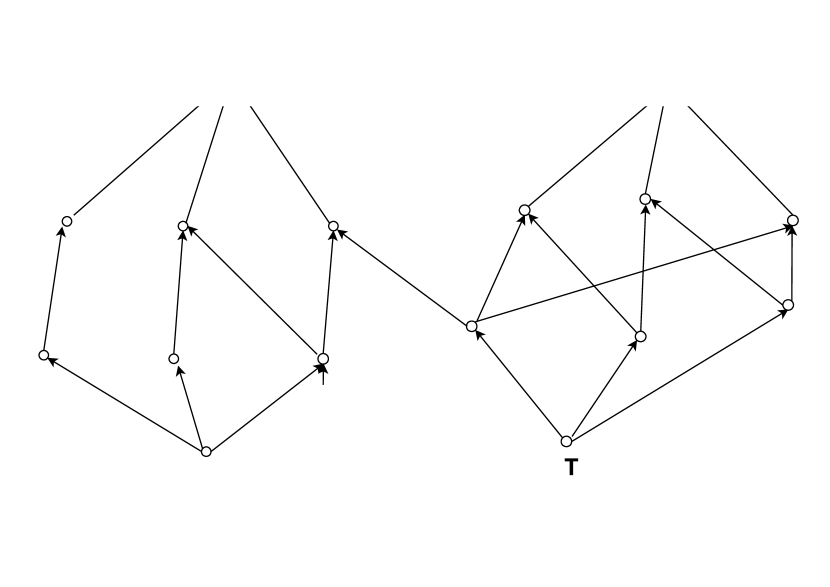
Figure 1. Example of possible connections between a topic $T$ and two sinks $S_{1}$ and $S_{2}$. Arrows originating from any node always point upwards, i.e. to the node hypernyms. The shortest path is 3 edges long for both sinks. In this and in all other figures of this section, possible links to co-hyponyms are not shown at any hypernymy level to simplify the reading.

As an example, consider Figure 1 where a portion of the Wikipedia tree is depicted, showing a topic $T$ that can be connected to two sinks $S_{1}$ and $S_{2}$. In such a figure, every link points to a node associated to a concept with a higher hypernymy with respect to the hypernymy of the term related to the node where the link originates. In other words, each link is oriented in a direction corresponding to a higher level of hypernymy. In Figure 1, the lengths $l_{p}(T,S_{1})$ and $l_{p}(T,S_{2})$ of the shortest path between $T$ and $S_{1}$ and $S_{2}$ respectively is 3 for both sinks. Consequently, no matter how $l_{p}(T,S_{1})$ and $l_{p}(T,S_{2})$ are combined, we would always argue that $T$ is related in the same way to both $S_{1}$ and $S_{2}$, as long as only $l_{p}(T,S_{1})$ and $l_{p}(T,S_{2})$ enter into play. However, the topology of the graph would suggest that the relatedness $w(T,S_{1})$ between $T$ and $S_{1}$ should be stronger than that between $T$ and $S_{2}$. In fact, if one started from node $T$ and made random upward moves (thus constantly increasing the hypernymy level), the probability of ending up in node $S_{1}$ would be higher than that of ending in node $S_{2}$ since there are more “upward-pointing” paths connecting $T$ to $S_{1}$ than to $S_{2}$. By “upward-pointing” paths, we mean paths exclusively made up of links oriented in a direction corresponding to a higher level of hypernymy.
Figure 1 suggests to take into account not only the length of the shortest path between a topic $T$ and a sink $S$ but also the overall number $n_{p}(T,S)$ of such “upward-pointing” paths connecting $T$ to $S$: the larger $n_{p}(T,S)$, the stronger the relatedness. Still in Figure 1, one would have $n_{p}(T,S_{1})=6$ and $n_{p}(T,S_{2})=1$ and, therefore, $T$ would turn out to be more strongly related to $S_{1}$ than to $S_{2}$, as expected. “Upward-pointing” paths are an example of those topological features, asymmetric in hypernymy, we were referring to early on as an instrument we could leverage to possibly improve the accuracy of the specific kind of relatedness measurement targeted by this study.
Considering again a given topic $T$ and recalling that there are $N_{s}$ sinks available altogether, the formula we propose to measure the relatedness $w(T,S_{m})$ of $T$ to the $m^{th}$ sink reads

(3) $$w(T,S_{m})=\bigg{(}\frac{n_{p}(T,S_{m})}{n_{tot}(T)}e^{-\alpha\big{[}l_{p}(T,S_{m})-l_{MIN}(T)\big{]}}\bigg{)}/N_{R}(T)\ ,$$

where $\alpha>0$, $l_{MIN}(T)=min_{i}\{l_{p}(T,S_{i})\ |\ \forall i\in[1,N_{s}]\}$,
$n_{tot}(T)=\sum_{m=1}^{N_{s}}n_{p}(T,S_{m})$ and where the normalization term $N_{R}(T)$ is given by

(4) $$N_{R}(T)=\sum_{m=1}^{N_{s}}\frac{n_{p}(T,S_{m})}{n_{tot}(T)}e^{-\alpha\big{[}l_{p}(T,S_{m})-l_{MIN}(T)\big{]}}\ .$$

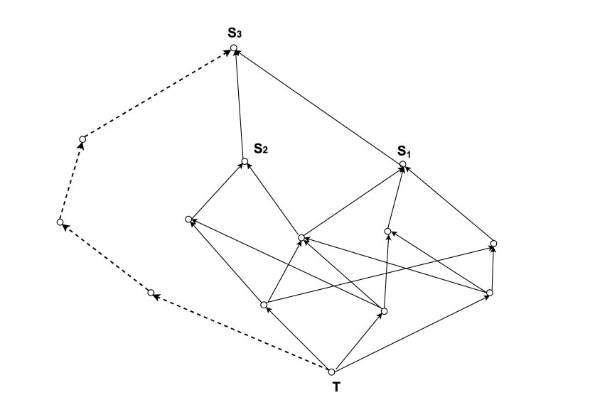
Figure 2. Example of path dismissal. The only path connecting topic $T$ to sink $S_{3}$ is the dashed one since the remaining two paths are discarded given that another sink is previously found along them.

According to Eq.(3), any weight $w(T,S_{m})$ results from the interplay between the number of “upward-pointing” paths connecting topic $T$ to sink $S_{m}$ and the corresponding LSP. The latter topological feature actually enters not through its “absolute” value but, rather, via its size relative to the minimum $l_{MIN}(T)$ of the lengths of the shortest paths between $T$ and any preset category. In this way, the strength of $w(T,S_{m})$ somehow depends on the comparison between different sinks — a key aspect when carrying out the profiling, as pointed out before.
Some remarks are now due.
First, in order to avoid to link a topic $T$ with a sink $S$ too far away, a maximal path length $l_{max}$ is introduced, i.e. paths between $T$ and any sink whose length is larger than $l_{max}$ are discarded in computing any weight $w$. It is true that the relatedness between $T$ and a distant sink $S$ gets exponentially suppressed according to Eq.(1), but $n_{p}(T,S)$ might be large in this case: thus, it might counterbalance — partially, at least — the exponential dump and result in an unwanted (albeit small, perhaps) perturbation.
As an example of this phenomenon taken from the Italian version of Wikipedia, let’s consider the topic “Thor”, the god of Nordic mythology. If $l_{max}$ is set to 6 and the parameter $\alpha$ in Eq.(3) is set to $3$, the only two categories (among those cited in footnote 3) whose weight is higher than 1% are “Religion” (scoring 88.2%) and “Politics” (11.8%). While the former appears quite naturally (Thor is a divinity and, as such, he can be obviously associated to “Religion”), the latter has a somehow less intuitive connection (“Politics” actually shows up since Thor is a god of war and war can be deemed as a political activity). With such a setup, i.e., $l_{max}=6$ and $\alpha=3$, $l_{p}(``Thor",``Religion")=l_{p}(``Thor",``Politics")=4$ while $n_{p}(``Thor",``Politics")=2$ and $n_{p}(``Thor",``Religion")=15$. If $l_{max}$ is increased to 10 while keeping $\alpha$ fixed, weights change since “Religion” and “Politics” now score 69.2% and 30.2% respectively. The reason is that, while $l_{p}(``Thor",``Religion")$ and $l_{p}(``Thor",``Politics")$ keep on being equal to 4, now $n_{p}(``Thor",``Politics")=7$ while $n_{p}(``Thor",``Religion")=16$. In other words, $n_{p}(``Thor",``Religion")$ essentially has not changed while $n_{p}(``Thor",``Politics")$ has become more than three times larger than it was before, thus resulting in an increase in importance of the spurious — to some extent — category. Consequently, in a case like this, setting $l_{max}$ equal to a short rather than to a large value does seem to yield more reasonable results.
Second, in case there are no paths with length shorter than $l_{max}$ connecting a topic to any of the sinks, $l_{max}$ is increased by one unit temporarily and just for that topic as long as at least a sink is encountered: this avoids the lack of mapping for some topics and the resulting loss of information about the user’s interests.
Third, once that a sink $S$ is encountered along a path, no further move upwards is considered along it, even though the length of such a path leading to $S$ is less than $l_{max}$. For example, assuming $l_{max}=4$, in Figure 2, the only path connecting $T$ to sink $S_{3}$ is the one whose edges are dashed, since the remaining two links incident to $S_{3}$ are dismissed given that they belong to paths — starting from $T$ — along which other sinks have already been found. The main reason for this choice is given by the fact that sinks might not necessarily be at the same height along the tree, i.e. some sinks might belong to the hypernyms of another sink. As an example, consider the sinks “Music” and “Arts”: though the latter is a hypernym of the former, the span of “Music” in the real world (that is, the space devoted to it on the media, the attention on the part of the audience, the amount of resources invested in it, etc.) compared to that of, say, “Ceramics” is so much wider that we might very well want to consider “Music” a sink on its own while merging “Ceramics” into the more generic “Arts” sink. In such a situation any path connecting a topic $T$ to “Music” whose length is shorter than $l_{max}$ could easily be prolonged to reach “Arts”, therefore establishing a connection between the latter and $T$. Such a connection would not obviously be wrong but, by increasing $w(T,\text{``Arts''})$, it will automatically weaken $w(T,\text{``Music''})$, which constitute an undesired effect given that “Music” is assumed to be a sink on its own.

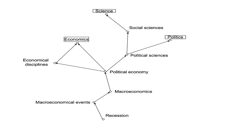
Figure 3. Example of a computation of relatedness taken from the Italian version of Wikipedia. Starting from the node associated to the concept of “Recession” (at the bottom), all edges belonging to paths leading to the sinks “Economics”, “Politics” and “Sciences” are shown. Other 15 sinks — spanning a wide variety of fields and listed in footnote 3 — were also considered but no paths leading to them and long 6 edges at most were found.

In summary, the algorithm for profiling a user $u$ starting from his/her topic map goes as follows:

1. a list of sinks $(S_{1},S_{2},\ldots,S_{N_{s}})$ is built, a value for parameters $\alpha$ in Eq.(1), $l_{max}$ and $l_{th}$ is chosen and a cycle over the topics in $u$’s topic map is introduced;

2. for each topic $T$ in the cycle, paths between $T$ and the sinks with length not exceeding $l_{max}$ are built, bearing in mind that any further move upwards along a path has to be dismissed as soon as a sink is encountered, irrespective of the current length of the path;

3. in case no paths as those described in step 2 are found, $l_{max}$ is temporarily increased by one unit as long as either any valid path connecting $T$ to at least one of the sinks is found or a given threshold $l_{th}$ is reached; afterwards, $l_{max}$ is brought back to its initial value;

4. the relatedness of $T$ to each sink is computed by means of Eq.(3);

5. finally, sinks are ranked on the basis of the scores defined in Eq.(1).

As an illustrative example, let us consider the categorization of the concept “Recession” based on the Italian version of Wikipedia. The resulting graph is shown in Figure 3, where, setting again $l_{max}=6$ and $\alpha=3$, we represent all the edges belonging to paths leading from the concept of “Recession” (“R”) at the bottom to the sinks “Economics” (“E”), “Politics” (“P”) and “Sciences” (“S”). No other sinks in the list detailed in footnote 3 can be reached with $l_{max}=6$. Making use of the notations introduced earlier, with reference to Figure 3 one has $n_{p}(\text{``R''},\text{``E''})=2$, $n_{p}(\text{``R''},\text{``P''})=1$, $n_{p}(\text{``R''},\text{``S''})=1$, $l_{p}(\text{``R''},\text{``E''})=4$, $l_{p}(\text{``R''},\text{``P''})=5$, $l_{p}(\text{``R''},\text{``S''})=6$ and, thus, $n_{tot}(\text{``R''})=4$ and $l_{tot}(\text{``R''})=4$. Consequently, the normalization factor $N_{R}(\text{``R''})$ and the relatedness $w$ of “Recession” to the three sinks are given by

$$N_{R}(\text{``R''}) = \frac{1}{2}+\frac{1}{4}e^{-3}+\frac{1}{4}e^{-6}\approx 0.51\ ,$$

$$w(\text{``R''},\text{``E''}) = \frac{1}{2}/N_{R}(\text{``R''})\approx 0.98\ ,$$

$$w(\text{``R''},\text{``P''}) = \frac{1}{4}e^{-3}/N_{R}(\text{``R''})\approx 0.02\ ,$$

(5) $$w(\text{``R''},\text{``S''}) = \frac{1}{4}e^{-6}/N_{R}(\text{``R''})\approx 0\ .$$

3. Implementation

We developed a prototypical implementation of the algorithm devised in the previous section, in the form of a Python library using the functionality provided by our Tapoi platform for the collection of online user activities and the generation and aggregation of the topic maps. Tapoi makes use of the commercial Dandelion APIs for entity extraction.
To speed up the computation, a dump of the Italian version of the Wikipedia tree has been downloaded and stored in a standard relational database management system, with the Python code interfacing directly with said database, thereby bypassing Wikipedia APIs.
Though at the moment the prototype makes use of the tree underpinning of the Italian version of Wikipedia, the analysis can be easily extended to other languages. In fact, Dandelion APIs automatically detect the language(s) used in a user’s social media activities and set topic labels accordingly within the corresponding topic map. At this point, it is enough to download the dump of Wikipedia in the very same language and make the Python code we implemented interact with such a dump. In case a topic map features more than a language, the Python code will interface all corresponding dumps and aggregate the resulting information.

4. Evaluation

If the main goal of the algorithm described in this paper had been relatedness measurement, we could have evaluated its soundness and performances by relying on the typical strategy followed when an algorithm tackling relatedness measurement is designed. In such cases, performances are usually evaluated by computing Pearson’s correlation coefficient $r$ or Spearman’s correlation coefficient $\rho$ between the algorithm predictions and human judgements. With respect to this practice, standard datasets that are typically employed are, for example, the lists by Miller & Charles (Miller and Charles, 1991) and by Rubenstein & Goodenough (Rubenstein and Goodenough, 1965).
However, as already stressed in Section 1, the actual purpose of the present work is customer profiling: not only this means that relatedness measurement is just a preliminary step, but it also results in the fact that, when relatedness has actually to be measured in the process, the terms involved usually lie several levels of hypernymy far one from the other. The datasets mentioned before — and similar ones — are typically made up of terms whose hypernymy relations do not own the features we want to focus on. Consequently, in order to apply our algorithm to such datasets, we would be compelled to completely pervert the nature of the algorithm itself and engineer an entirely new one, drifting apart from our main goal.
In order to evaluate the performances of our algorithm in a way consistent with its purpose and also to find the best values for the model parameters $\alpha$, $l_{max}$ and $l_{th}$ defined in Section 2, we decided to apply our algorithm to the topic maps extracted from a set $C$ made up of $N_{c}$ Twitter accounts, for each one of which the content of the activities should be strongly oriented towards a given category (referred to as “ground-truth sink” and labelled $S_{gt}$ in what follows). For example, activities on a sportsman’s account are likely to mostly deal with sport while topics extracted from the account of an association of literary critics should be related to literature to a great extent. The idea is to measure how well our algorithm is capable of identifying the $S_{gt}$ ideally associated to each account when varying the model parameters. This measurement can be carried out by means of some indices summarizing the average degree of correctness on set $C$ as a whole.
Before introducing such indices, for later convenience we label with $C_{i}$ the subset of $C$ made up of those accounts whose ground-truth sink is category $S_{i}$ (with $i\in\{1,2,\ldots,N_{s}\}$, being $N_{s}$ the number of categories) and with $n_{i}$ the cardinality, i.e., the number of elements, of $C_{i}$. After extracting a topic map from each account, setting the model parameters $\alpha,l_{max},l_{th}$ to some tentative values and computing the percentages in Eq.(1) for each account, the indices taken into account for evaluating the quality of the predictions — called score ($SC$), rank ($RK$) and difference ($\Delta$) — are defined as

$$SC = \frac{1}{N_{s}}\sum_{i=1}^{N_{s}}sc(S_{i})\ ,$$

$$RK = \frac{1}{N_{s}}\sum_{i=1}^{N_{s}}rk(S_{i})\ ,$$

(6) $$\Delta = \frac{1}{N_{s}}\sum_{i=1}^{N_{s}}\delta(S_{i})\ ,$$

with

$$sc(S_{i}) = \frac{1}{n_{i}}\sum_{a_{j}\in C_{i}}sc(a_{j})\ ,$$

$$rk(S_{i}) = \frac{1}{n_{i}}\sum_{a_{j}\in C_{i}}rk(a_{j})\ ,$$

(7) $$\delta(S_{i}) = \frac{1}{n_{i}}\sum_{a_{j}\in C_{i}}\delta(a_{j})\ ,$$

where $i\in\{1,2,\ldots,N_{s}\})$, $a_{j}$ labels a given Twitter account and quantities $sc(a_{j})$, $rk(a_{j})$ and $\delta(a_{j})$ associated to account $a_{j}$ are defined as follows

• $sc(a_{j})$ is equal to score $pc(u_{j},S_{gt}(a_{j}))$ defined in Eq.(1), where $S_{gt}(a_{j})$ is the ground-truth sink associated to account $a_{j}$ and $u_{j}$ is its owner;

• $rk(a_{j})$ is the ranking of the ground-truth sink $S_{gt}(a_{j})$ on the basis of the percentages computed according to Eq.(1) starting from the topic map extracted from $a_{j}$: if sink $S_{gt}(a_{j})$ gets the highest score, then $rk(a_{j})=1$, if it obtains the second highest, then $rk(a_{j})=2$, and so on;

• $\delta(a_{j})$ is defined as

  (8) $$\delta(a_{j})=\frac{pc(u_{j},S_{gt}(a_{j}))-pc(u_{j},S_{*}(a_{j}))}{pc(u_{j},S_{gt}(a_{j}))}\ ,$$

  where $pc(u_{j},S_{*}(a_{j}))$ corresponds to the largest value among the percentages $pc(u_{j},S_{m})$’s for all $m$ categories (in case the largest value is not $pc(u_{j},S_{gt}(a_{j}))$, i.e., in case the ground-truth category is not ranked first) or to the second largest value among the $pc(u_{j},S_{m})$’s (in case $S_{gt}(a_{j})$ is ranked first).

Some remarks are now due.
$SC$, $RK$ and $\Delta$ are all defined through a “double average”: a first average — that in Eqs.(4) — is computed within each subset $C_{i}$, i.e., on all Twitter accounts sharing a common ground-truth sink, while a second — in Eqs.(6) — is evaluated on the different categories starting from the mean values obtained in Eqs.(4). The rationale is that one wants to set all sinks on the same footing before evaluating score, rank and difference: if one had computed the plain average on all the $N_{c}$ topic maps, those categories that are ground truth for (relatively) many accounts in the set $C$ would have had more weight, thus making the indices “artificially” high or low, depending on how well or bad these over-represented categories emerge within the corresponding subsets $C_{i}$’s. The “pre-average” in Eqs.(4) gives each category a single vote in Eqs.(6) — so to speak —, and any “artificial” increase (or decrease) in $SC$, $RK$ and $\Delta$ should in principle be avoided.
As for the meaning of the indices, loosely speaking $SC$ essentially measures the average share of activities that, for each account, can be related to the corresponding ground-truth sink $S_{gt}$. Bearing in mind that, by virtue of Eq.(1), such a share ranges from 0 to 1, in the ideal case when all activities are associated solely to $S_{gt}$ for all accounts, then $SC=1$; conversely, in the opposite case when no activities can be related to $S_{gt}$ on any account at all, $SC$ would be equal to 0. Thus, the closer $SC$ to 1, the better. However, $SC$ will never be exactly equal to 1, partly because — in general — topics are usually related to different categories (though with different degrees of relatedness), partly because it is quite natural that a user has typically more than one interests — there might be a sink that stands out given perhaps its relation to the user’s job (we are assuming that such a category is $S_{gt}$), but other ones will usually be featured in his/her activities.
In themselves, the individual $sc(a_{j})$’s out of which $SC$ is eventually computed are a sort of absolute measurement, i.e. they do not convey any explicit information about the way $S_{gt}$ compares with the other categories that are supposed to relate less than $S_{gt}$ to the topic map extracted from a given account. For example, an apparently low value of $sc(a_{j})$ might nevertheless correspond to the highest of the percentages $pc(u_{j},S_{m})$, especially for a Twitter account whose activities are rather sparse category-wise. Conversely, the ground-truth sink might get an apparently high share — say, slightly lower than 0.5 — but it might be preceded by another category whose score is actually above 0.5. Quantities $rk(a_{j})$’s entering the computation of $RK$ overcome these inconveniences since they explicitly yield the rank of $S_{gt}$, irrespective of whether the corresponding $sc(a_{j})$’s are seemingly high or low. In the ideal case when $S_{gt}$ is ranked first on all accounts, the overall $RK$ will be equal to 1, otherwise it will be (increasingly) higher, thus signalling that, for a (larger and larger) number of accounts, the ground-truth sink does not actually get ranked in the first position.
Finally, though $rk(a_{j})$ provides a comparison between $S_{gt}$ and all other categories on account $a_{j}$, still it does not measure the gap between the ground-truth sink and the remaining ones. For example, on a given account $a_{j}$, $rk(a_{j})$ will be equal to 1 if $S_{gt}$ gets ranked first, irrespective of whether this occurs by a large margin or by a very tiny one. On the contrary, $\delta(a_{j})$ is defined in a such a way to have very different values in the case $S_{gt}$ clearly stands out and in the case it is ranked first by a narrow margin. In fact, according to Eq.(8), $\delta(a_{j})$ reads 1 when the score $pc(u_{j},S_{m})$ is zero for all categories except for the ground-truth sink (this would be the ideal, though hardly-reachable scenario), but it gets negative as soon as $S_{gt}$ is not ranked first — the larger the gap between the ground-truth category and the category ranked as the first one, the more negative $\delta(a_{j})$. Such features are reflected in the overall index $\Delta$ which will read 1 in the above-mentioned ideal scenario and be (increasingly) negative as soon as, on a (wider and wider) bunch of accounts, $S_{gt}$ is not ranked first by a large margin with respect to the leading sink.
Bearing these observations in mind, we profiled $N_{c}=89$ accounts altogether, shared among 14 out of the $N_{s}=18$ categories we currently include in our study, trying to diversify — for each category – the kind of user. For instance, in profiling accounts related to sink “Cinema”, we considered not only accounts owned by actors/actresses or directors, but also those run by producers. Similarly, while focusing on category “Music”, we analyzed the accounts of artists belonging to different genres (rock, hip hop, etc.), of fan clubs and of those institutions — like theaters — often hosting music events.
We computed $SC$, $RK$ and $\Delta$ for several setups of the model parameters $\alpha$, $l_{max}$ and $l_{th}$ and found out that the best results are obtained with $\alpha=3$, $l_{max}=6$ and $l_{th}=12$ for all the three performance indices: more precisely, we get $SC=0.29$, $RK=1.21$ and $\Delta=0.32$. Roughly speaking, on average $S_{gt}$ can be associated to more than one fourth of the activities of an account, it gets ranked first in 4 out of 5 cases (in the fifth case, it is ranked as the second sink) and its percentage is approximately $10\%$ higher than that of the strongest competitor sink-wise.
For the optimal values of the model parameters quoted before, plots in Figure 4 show the values of observables $sc(S_{i})$, $rk(S_{i})$ and $\delta(S_{i})$ defined in Eqs.(4) for all 14 categories eventually taken into account in the process of performance evaluation. Each panel of Figure 4 displays the categories on the horizontal axis; the upper panel shows, for each category $S$, the average score of such category as computed on the topic maps extracted from those Twitter accounts having $S$ as ground-truth sink. For example, on the topic maps obtained from the 6 accounts that should mostly refer to “Science”, the average score of “Science” reads slightly less than 0.45. Similarly, the middle (lower) panel of Figure 4 displays the average ranking (difference) of each sink $S$ obtained from the activities of the Twitter accounts that should be oriented towards $S$. For instance, since, on the 10 accounts that should refer to “Economics”, such a sink is ranked first on 9 accounts and second on the remaining one, $rk(``Economics")=1.1$ (i.e., $rk=(1+1+1+1+1+1+1+1+1+2)/10=1.1$), as shown in the middle panel of Figure 4.

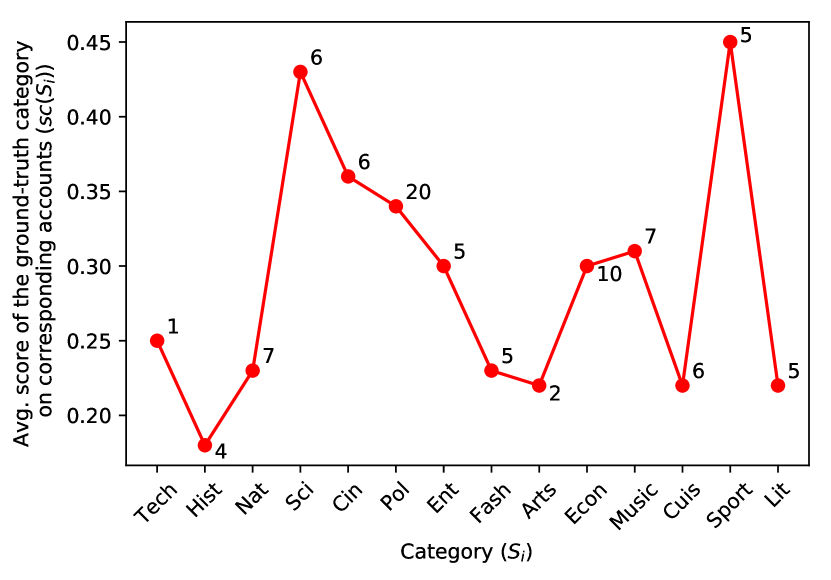
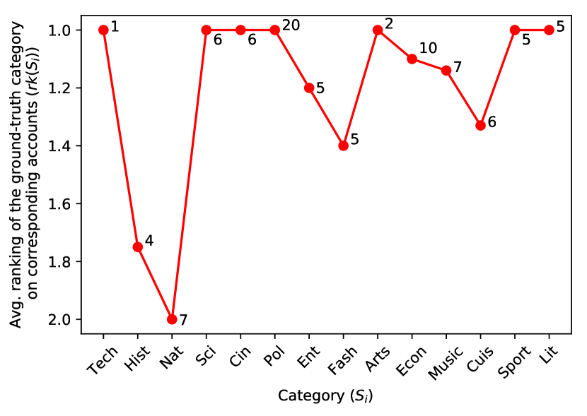
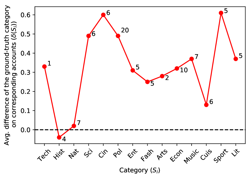
Figure 4. Plots of $sc(S_{i})$, $rk(S_{i})$ and $\delta(S_{i})$ as defined in Eqs.(4) for 14 categories. For each category $S_{i}$, the plots display — from up to bottom — the average score, ranking and difference of $S_{i}$ as computed from the topic maps extracted from the Twitter accounts that should have $S_{i}$ as ground-truth sink. The number of Twitter accounts supposedly having $S_{i}$ as ground-truth sink is shown close to each point.
    The categories — displayed on the horizontal axis of each panel — are “Technology and applied sciences” (Tech), “History” (Hist), “Nature” (Nat), “Science” (Sci), “Cinema” (Cin), “Politics” (Pol), “Entertainment” (Ent), “Fashion” (Fash), “Arts” (Arts), “Economics” (Econ), “Music” (Music), “Cuisine” (Cuis), “Sport” (Sport) and “Literature” (Lit).

Figure 5 delves into the ranking of $S_{gt}$ within the corresponding subset $C_{i}$, i.e., it shows — for each category $S_{i}$ — the percentage of accounts, computed on the subset where $S_{i}$ is supposed to be the ground-truth sink, on which $S_{i}$ is ranked first or within the first two or three categories on the basis of the score $pc$ defined in Eq.(1). It can be seen that there are seven categories — i.e., “Literature”, “Sport”, “Arts”, “Politics”, “Cinema”, “Science” and “Technology and applied sciences” — that are ranked first on all accounts whose activities are supposedly mostly oriented towards them, i.e., on all accounts belonging to the correponding subset $C_{i}$. At worst, the ground-truth sink is ranked at the third position: this occurs for four accounts (two of them associated to category “Nature”, one to “History” and one to “Fashion”) while, on all other accounts, $S_{gt}$ is always ranked within the first two positions.
For some categories, the picture looks very good. For instance, in the 5 accounts whose ground-truth sink is supposed to be “Sport”, not only this sink is always ranked as the first one, but, on average, 45% of the activities can be related to it alone while the second-ranked category is associated to (roughly) 17% of the extracted topics (this latter info can be loosely obtained by combining the results for “Sport” in the upper and in the lower plot in Figure 4). In other words, as expected “Sport” clearly stands out in the activities extracted from the corresponding accounts. A similar situation holds for other sinks, like “Science” and “Cinema”.
On the opposite side lie categories like “History”. In fact, in the 4 accounts supposedly related to it, less than 20% of activities can be associated to such a sink which is ranked first only in two cases. This poor scenario is also reflected in $\delta(``History")$, which lies below the threshold — corresponding to the dashed line in the lower plot of Figure 4 — separating the categories for which the ground-truth sink is mostly ranked first (this resulting in a $\delta$ with positive sign) from those for which this does not hold.
In order to cast some light on the bad results obtained for some sinks, we are currently “manually” checking the topic maps extracted from the accounts supposedly related to such bad-behaving categories. By this approach, we aim at assessing to which extent the fault is in the model architecture rather than in our initial assumptions on these accounts — in fact, they might be (much) less related to the ground-truth sink than supposed a priori.

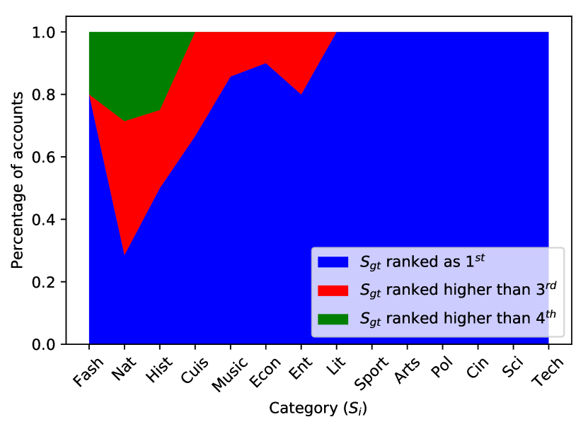
Figure 5. For each category $S_{i}$, the percentage of accounts where $S_{i}$ is ranked as first (blue) or within the first two (red) or three (green) positions is displayed. The percentage is computed on the subset referred to in the text as $C_{i}$, i.e., on the subset of accounts for which $S_{i}$ is supposed to be the ground-truth category. The labels for the categories on the horizontal axis are explained in the caption of Figure 4.

5. Conclusions

In this paper we described an algorithm to carry out the profiling of a user starting from his/her activities on social media, leveraging on the so-called social login. This algorithm makes use of the Wikipedia ontology to project the concepts referred to in such activities onto a predefined set of categories and employs the resulting map to profile the user’s interests. A preliminary implementation — in the form of a Python library using a dump of the Italian version of Wikipedia — has been developed and its performances are currently being tested on a series of benchmark Twitter accounts whose activities should be strongly oriented towards a specific category.
The next stage of our work will involve further checks on the model performances, the extension of the existing library in order to be able to handle languages other than Italian and the eventual inclusion of the algorithm into a commercial software for customer profiling.

Acknowledgements — This project has received funding from the European Union’s Horizon 2020 research and innovation programme under grant agreement No 739783 (DataSci4Tapoi).
The information and views set out in this study are those of the author(s) and do not necessarily reflect the official opinion of the European Union. Neither the European Union institutions and bodies nor any person acting on their behalf may be held responsible for the use which may be made of the information contained therein.

References

- (1)
- Hirst and St-Onge (1998) G. Hirst and D. St-Onge. 1998. Lexical chains as representations of context for the detection and correction of malapropisms. In WordNet: An Electronic Lexical Database. C. Fellbaum, Cambridge, Mass.: MIT press, 305–332.
- Jarmasz and Szpakowicz (2003) M. Jarmasz and S. Szpakowicz. 2003. Roget’s Thesaurus and semantic similarity, Proc. of RANLP-03, 212-219. (2003).
- Landgrebe and Duin (2007) S.C.W. Landgrebe and R.P.W. Duin. 2007. Approximating the multiclass ROC by pairwise analysis. Pattern Recognition Letters 28 (2007), 1747–1758.
- Leacock and Chodorow (1998) C. Leacock and M. Chodorow. 1998. Combining local context and WordNet similarity for word sense identification. (1998).
- Miller and Charles (1991) G. A. Miller and W. G. Charles. 1991. Contextual correlates of semantic similarity, Language and Cognitive Processes, 6(1):1–28. (1991).
- Ponzetto and Strube (2006) S.P. Ponzetto and M. Strube. 2006. WikiRelate! Computing Semantic Relatedness Using Wikipedia, AAAI’06 proceedings of the 21st national conference on Artificial intelligence, 1419-1424. (2006).
- Ponzetto and Strube (2007) S.P. Ponzetto and M. Strube. 2007. Knowledge Derived From Wikipedia For Computing Semantic Relatedness. Journal of Artificial Intelligence Research 30 (2007), 181–212.
- Rada et al. (1989) R. Rada, H. Mili, E. Bicknell, and M. Blettner. 1989. Development and application of a metric to semantic nets, IEEE Transactions on Systems, Man and Cybernetics, 19(1):17-30. (1989).
- Rubenstein and Goodenough (1965) H. Rubenstein and J. Goodenough. 1965. Contextual correlates of synonymy, Communications of the ACM, 8(10):627–633. (1965).
- Segall and Greenstadt (2013) J. Segall and R. Greenstadt. 2013. The illiterate editor: metadata-driven revert detection in Wikipedia, Proceedings of the 9th International Symposium on Open Collaboration (WikiSym 13). (2013).
- Witten and Milne (2008) I. Witten and D. Milne. 2008. An effective, low-cost measure of semantic relatedness obtained from Wikipedia links, Proceedings of the AAAI 2008 Workshop on Wikipedia and Artificial Intelligence (WIKIAI 2008). (2008).
- Wu and Palmer (1994) Z. Wu and M. Palmer. 1994. Verb semantics and lexical selection, Proc. of ACL-94, 133-138. (1994).