A microscopic field theoretical approach for binary mixtures of active and passive particles

Abstract

We consider a phase field crystal modeling approach for binary mixtures of interacting active and passive particles. The approach allows to describe generic properties for such systems within a continuum model. We validate the approach by reproducing experimental results, as well as results obtained with agent-based simulations, for the whole spectrum from highly dilute suspensions of passive particles to interacting active particles in a dense background of passive particles.

I Introduction

Active systems have been in the focus of intense research for the last decade because they provide deep insights into the self-organization of systems that are intrinsically in a non-equilibrium state such as living matter. Even more interesting are mixtures of active and passive particles. Situations of active particles in crowed environments or passive particles in an active bath resemble the situation in living matter more realistically and might even shed light on the active dynamic processes within a cell Das, Polley, and Rao (2016). Observed phenomena in mixtures of active and passive particles are e.g. activity-induced phase-separation Stenhammar et al. (2015), the formation of large defect-free crystalline domains Kümmel et al. (2015), propagating interfaces Wysocki, Winkler, and Gompper (2016) but also a transition from diffusive to subdiffusive dynamics Zeitz, Wolff, and Stark (2017); Morin et al. (2017a) and suppressed collective motion Morin et al. (2017b). To understand this wide span of phenomena is crucial to almost all applications of active systems.

Different ways exist to describe phenomena in active systems theoretically. Typical approaches for active systems consider either the microscopic scale, taking the interactions between the particles into account, or the macroscopic scale, focusing on the emerging phenomena. For reviews on both theoretical descriptions see e.g. Marchetti et al. (2013); Ramaswamy (2010). Examples for extensions towards mixtures of active and passive particles are summarized in Bechinger et al. (2016) and range from active particles in confined domains Briand, Schindler, and Dauchot (2017); Lushi and Peskin (2013); Wioland et al. (2013), through active particles moving between fixed or moving obstacles Reichhardt and Reichhardt (2017, 2018); Kaiser, Wensink, and Löwen (2012); Kaiser et al. (2013); Zeitz, Wolff, and Stark (2017), to binary mixtures of interacting active and passive particles McCandlish, Baskaran, and Hagan (2012); Kümmel et al. (2015); Stenhammar et al. (2015); Wysocki, Winkler, and Gompper (2016). All these studies are examples for models on the microscopic scale. In Menzel and Löwen (2013); Alaimo, Praetorius, and Voigt (2016) a continuum modeling approach was introduced for active systems which combines aspects from the microscopic and the macroscopic scales. The goal of the paper is to extend this approach to mixtures of active and passive particles which will allow to describe generic properties of such systems. We use the model to study the effect of a few active particles in passive systems (active doping) Kümmel et al. (2015); Ni et al. (2014); van der Meer, Dijkstra, and Filion (2016) and how passive particles perturb collective migration in an active bath Wu and Libchaber (2000); Valeriani et al. (2011); Hinz et al. (2014); Zeitz, Wolff, and Stark (2017). For the first case we observe enhanced crystallization in the passive system, in quantitative agreement with the results of Kümmel et al. (2015). For the active bath case we investigate how collective migration is affected by a disordered environment. For the special case of immobile passive particles these results are in agreement with Morin et al. (2017a, b). However, for mobile passive particles new phenomena and patterns emerge, which ask for experimental validation. Also the intermediate regime of similar fractions of active and passive particles is rich in complex phenomena but much harder to quantify.

II The Model

The starting point for the derivation of the model is the microscopic field theoretical model for active particles introduced in Alaimo, Praetorius, and Voigt (2016). It has been validated against known results obtained with minimal agent-based models and proven to be applicable for large scale computations. The model reads in scaled units

$$\begin{array}[]{l}\partial_{t}\psi=M_{0}\Delta\frac{\delta\mathcal{F}_{\rm vpfc}}{\delta\psi}-v_{0}\triangledown\cdot(\psi\mathbf{P})\\ \partial_{t}\mathbf{P}=\Delta\left(\alpha_{2}\mathbf{P}+C_{2}\mathbf{P}^{3}\right)-\left(\alpha_{4}\mathbf{P}+C_{4}\mathbf{P}^{3}\right)-v_{0}\mathbf{\triangledown}\psi-\beta\mathbf{P}\mathbbm{1}_{\psi_{A}\leq 0}\end{array}$$ (1)

for a one-particle density field $\psi(\bm{r},t)$, which is defined with respect to a reference density $\bar{\psi}$, and the polar order parameter $\mathbf{P}(\bm{r},t)$, which is related to a coarse-grained velocity field with a typical magnitude $v_{0}$ of the self-propulsion velocity. $\mathbf{P}$ is a local quantity that is different from zero only within the peaks of the density field $\psi$, which is ensured by $\beta>0$ typically larger than the other terms entering the $\mathbf{P}$ equation. $M_{0}$ is the mobility, $\alpha_{2}$ and $\alpha_{4}$ are two parameters related to relaxation and orientation of the polarization field and $C_{2}$ and $C_{4}$ are parameters which govern the local orientational ordering. For simplicity we will restrict ourselves to the case $C_{2}=C_{4}=0$, which only allows gradients in the density field $\psi$ to induce local polar order. The energy functional $\mathcal{F}_{\rm vpfc}=\mathcal{F}_{\rm pfc}+\mathcal{F}_{\rm v}$ consists of a Swift-Hohenberg energy Swift and Hohenberg (1977)

$$\mathcal{F}_{\rm pfc}=\int\left[\frac{1}{4}\psi^{4}+\frac{1}{2}\psi(q+(1+\Delta)^{2})\psi\right]d\mathbf{r},$$ (2)

with a parameter $q$ related to temperature and a penalization term

$$\mathcal{F}_{\rm v}=\int H(|\psi|^{3}-\psi^{3})d\mathbf{r},$$ (3)

with $H\simeq 1500$ to constrain the one-particle density field $\psi$ to positive values. The penalization term $\mathcal{F}_{\rm v}$ is the essential modification which allows to model individual particles Chan, Goldenfeld, and Dantzig (2009); Berry and Grant (2011); Robbins et al. (2012); Praetorius and Voigt (2015a). Without this additional term the model can be related to models for active crystals Menzel and Löwen (2013); Menzel, Ohta, and Löwen (2014). If, in addition, we neglect the coupling with the polar order parameter $\mathbf{P}$ we obtain the classical phase field crystal (PFC) model introduced in Elder et al. (2002); Elder and Grant (2004) to model elasticity in crystalline materials. For a detailed derivation of (2) and its relation to classical density functional theory we refer to Elder et al. (2007); van Teeffelen et al. (2009). If the coupling with $\mathbf{P}$ is neglected but the penalization term (3) considered, the model is known as the vacancy PFC (VPFC) model Chan, Goldenfeld, and Dantzig (2009).

Various ways have been introduced to extend the classical PFC model towards a second species, thus modeling binary mixtures Elder et al. (2007); Robbins et al. (2012). We adopt one of these approaches for the VPFC model by considering energies for species $A$ and $B$ with

$$\mathcal{F}(\psi_{A},\psi_{B})=\mathcal{F}^{A}_{\rm vpfc}(\psi_{A})+\mathcal{F}^{B}_{\rm vpfc}(\psi_{B})+\mathcal{F}_{\rm int}^{AB}(\psi_{A},\psi_{B})$$ (4)

where $\mathcal{F}^{i}_{\rm vpfc},i=A,B$ as before and

$$\mathcal{F}_{\rm int}^{AB}(\psi_{A},\psi_{B})=\frac{a}{2}\psi_{A}^{2}\psi_{B}^{2}$$ (5)

an interaction energy with $a>0$.

In principle both species appearing in (4) could be made active. Our aim is however to simulate binary mixtures of interacting active and passive particles. With this in mind we couple only species A to the polar order parameter $\mathbf{P}$. We further assume $\mathcal{F}^{A}_{\rm vpfc}=\mathcal{F}^{B}_{\rm vpfc}=\mathcal{F}_{\rm vpfc}$ and thus e.g. equal size of the active and passive particles. The resulting dynamical equations are

$$\begin{array}[]{ll}\frac{\partial\psi_{A}}{\partial t}=M_{0}^{A}\Delta\left(\frac{\delta\mathcal{F}(\psi_{A})}{\delta\psi_{A}}+a\psi_{A}\psi_{B}^{2}\right)-v_{0}\nabla\cdot(\psi_{A}\mathbf{P})\\ \partial_{t}\mathbf{P}=\alpha_{2}\Delta\mathbf{P}-\alpha_{4}\mathbf{P}-v_{0}\nabla\psi_{A}-\beta\mathbf{P}\mathbbm{1}_{\psi_{A}\leq 0}\\ \frac{\partial\psi_{B}}{\partial t}=M_{0}^{B}\Delta\left(\frac{\delta\mathcal{F}(\psi_{B})}{\delta\psi_{B}}+a\psi_{A}^{2}\psi_{B}\right)\end{array}$$ (6)

which define a microscopic field theoretical approach for binary mixtures of interacting active and passive particles. An extension to more than two species, species with different size and interaction potential and active species with different self-propulsion velocities is obvious.

III Results

We solve equations (6) in two dimensions using a parallel finite element approach Backofen, Rätz, and Voigt (2007). We adopt a block-Jacobi preconditioner Praetorius and Voigt (2015b) that allows us to use a direct solver locally. This is implemented in AMDiS Vey and Voigt (2007); Witkowski et al. (2015). The computational domain is a square of size $L=200$ with periodic boundary conditions. The initial condition for $\psi_{A}$ and $\psi_{B}$ is calculated using a one-mode approximation with lattice distance $d=4\pi/\sqrt{3}$ for each particle Praetorius and Voigt (2015a), with the centers placed randomly according to a packing algorithm Skoge et al. (2006). The $\mathbf{P}$ field is set to zero initially.

Each maxima in the one-particle density fields $\psi_{A}$ and $\psi_{B}$ is interpreted as an active or passive particle, respectively. The diameter of the particle is defined by the lattice distance $d$. We track the particle positions $\mathbf{x}^{i}_{A,B}(t)$ and use this information to compute the particle velocities $\mathbf{v}^{i}_{A,B}(t)$ as the discrete time derivative of two successive maxima. We define the total particle density $\phi=N\sigma/L^{2}$, with $N$ the total number of particles $N=N_{A}+N_{B}$ and $N_{A,B}$ the number of $A$ and $B$ particles, respectively. The parameter $\sigma=\pi(d/2)^{2}$ is the area occupied by a single particle. The relative density $\phi_{A}=N_{A}/N$ corresponds to the fraction of active particles present in the system. For low relative densities ($\phi_{A}<0.2$) we are in the regime of active doping, and analyse how a passive system is influenced by the presence of a few active particles. For high relative densities ($\phi_{A}>0.7$) we are in the regime of an active bath and study how a few passive particles affect an active system.

We fix the following parameters $(a,v_{0},\alpha_{2},\alpha_{4},\beta,H,q)=(200,1.5,0.2,0.1,2,1500,-0.9)$, unless otherwise specified in the figure captions.

III.1 Active doping: how active particles enhance crystallization

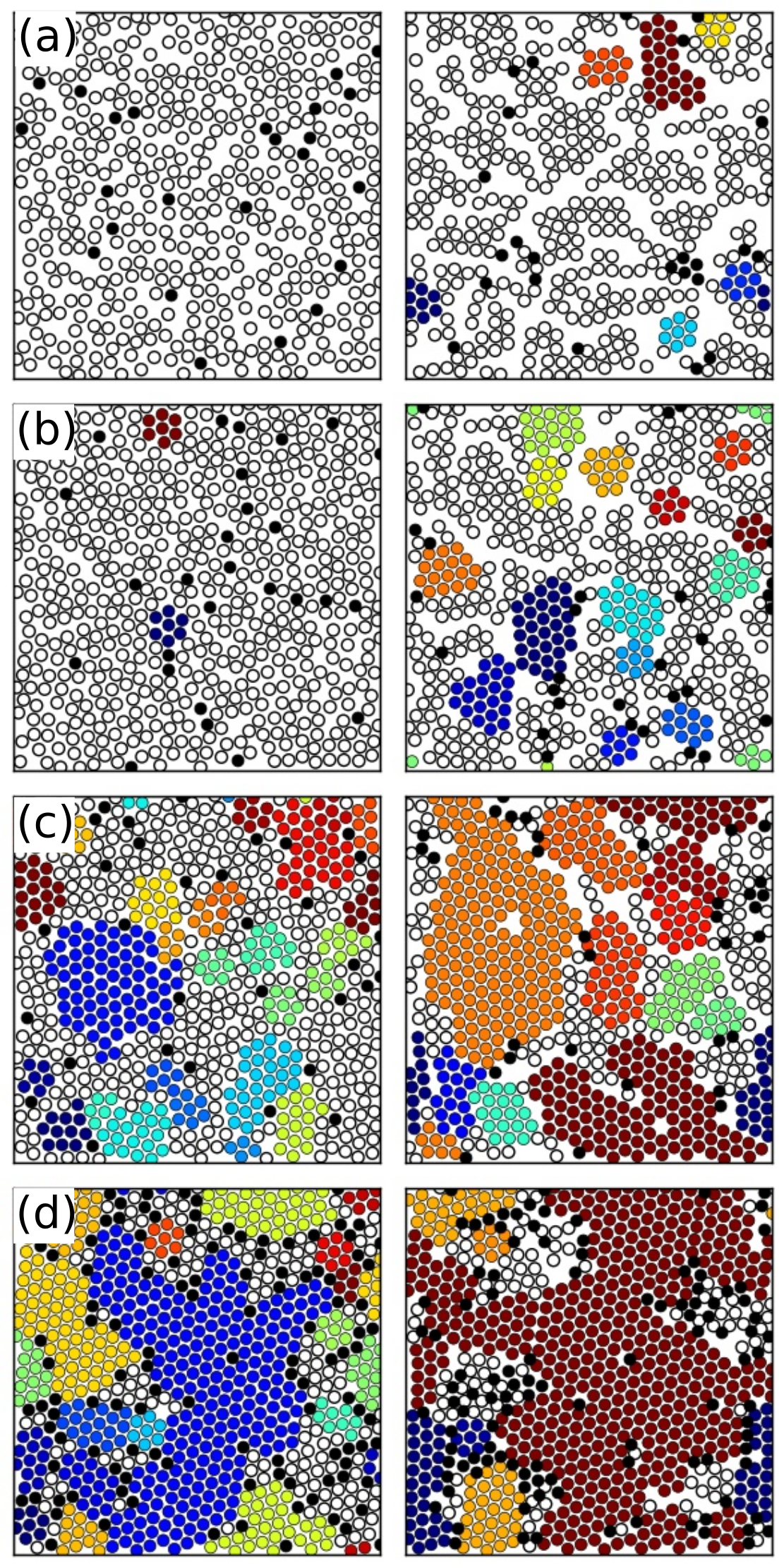
Figure 1: Snapshots showing passive clusters for different relative and absolute densities at time $t=0$ (first column) and at time $t=1000$ (second column). Particles with the same color belong to the same cluster, white disks represents passive particles not belonging to any cluster and black disks are active particles. (a) $\phi=0.5,\phi_{A}=0.05$, (b) $\phi=0.6,\phi_{A}=0.05$ (c) $\phi=0.7,\phi_{A}=0.05$, (d) $\phi=0.8,\phi_{A}=0.15$. Other parameters are $M_{0}^{A}=M_{0}^{B}=50$.

It has been shown by particle simulations Ni et al. (2014); van der Meer, Dijkstra, and Filion (2016) and experimentally Kümmel et al. (2015) that the crystalline structure of passive particles is altered by the presence of active agents. More precisely active particles generate density variation in the passive system and promote crystallization, leading to the formation of passive clusters. To analyze these phenomena with our microscopic field theoretical approach we need to identify if a particle belongs to a cluster. We follow the definition of Kümmel et al. (2015) where two criteria have to be fulfilled. The nearest neighbor distances less than $3/2d$ and the coordination number is $6$.

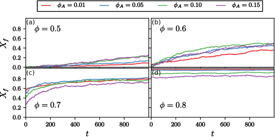
Figure 2: Percentage of passive particles belonging to a cluster $X_{f}$ as a function of time for different relative and absolute densities $\phi_{A}$ and $\phi$. We observe that for $\phi=0.5$ and $\phi=0.6$ (top row), increasing the number of active particles lead to an increase of $X_{f}$, whereas the opposite is true for $\phi=0.7$ and $\phi=0.8$ (bottom row). Other parameters are $M_{0}^{A}=M_{0}^{B}=50$. Each curve has been obtained as the average of five different simulations started with different initial conditions.

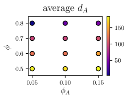
Figure 3: Average of the maximum displacement $d_{A}$ of active particles moving in a binary mixture for different values of $\phi$ and $\phi_{A}$. Active particles travel a longer distance when the passive particles have not crystallized, until the extreme case of $\phi=0.8$, $\phi_{A}=0.05$ where $d_{A}$ is so low that active particles are basically trapped (see also supplementary video). Other parameters are $M_{0}^{A}=M_{0}^{B}=50$. Each point has been obtained as the average of five different simulations started with different initial conditions.

Figure 1 shows snapshots with passive clusters for different relative and absolute densities, $\phi_{A}$ and $\phi$, respectively. The time evolution of the percentage of passive particles which belong to a cluster $X_{f}$ is shown in figure 2. For dilute systems ($\phi=0.5$, figure 1(a)) $X_{f}$ slowly increases with time. Increasing the relative density $\phi_{A}$ leads to larger values $X_{f}$. However, it remains relatively low, rarely exceeding $20\%$, for the considered time ($t=1000$). Increasing the density ($\phi=0.6$, figure 1(b)) the system changes from a state where no clusters are present ($t=0$) to a state where up to $50\%$ of the passive particles are found in clusters. A maximum $X_{f}$ is observed for $\phi_{A}=0.1$, where $X_{f}$ saturates at $t=1000$. Further increasing the number of active particles leads to a reduction of $X_{f}$. Adding more and more active particles to systems with already existing crystalline clusters introduces disorder. A phenomena already observed in Kümmel et al. (2015). By further increasing the density ($\phi=0.7$, figure 1(c)) some clusters are already present for the random initial configuration at $t=0$, due to spontaneously crystallization. Active particles can be inside these regions, thus disturbing their symmetry. This explains why the system behaves in the opposite way as for the dilute case, with $X_{f}$ decreasing as the fraction of active particles $\phi_{A}$ increases. Finally for $\phi=0.8$ the initial configuration is already almost completely crystallized ($X_{f}\simeq 1$ for $t=0$, figure 1(d)). Adding active particles partially destroys the crystalline structure (figure 2) and $X_{f}$ decreases for increasing $\phi_{A}$. We thus observe both phenomena, enhanced crystallization in dilute systems and suppressed crystallization in dense systems.

A final observation concerns how the dynamics of the active particles is affected by the presence of passive ones. In figure 3 the maximum displacement $d_{A}$ for active particles (averaged over all the particles) is shown as a function of the absolute and relative densities $\phi$ and $\phi_{A}$. No data is shown for $\phi_{A}=0.01$, as the number of active particles is too small for meaningful averages. We observe a clear correlation between $d_{A}$ and the crystallization in the system: the higher $X_{f}$, the smaller is the maximum displacement of active particles until, for the extreme case of $\phi=0.8$ and $\phi_{A}=0.05$ active particles are trapped inside a big cluster and have a very small maximum displacement (see also supplementary video).

III.2 Active bath: how passive particles can suppress collective migration

Inelastic collisions in systems which are composed solely of active particles can lead to collective motion. This has been shown by particle based models, e.g. Grossman, Aranson, and Ben Jacob (2008), microscopic field theoretical models Alaimo, Praetorius, and Voigt (2016) and phase field models Löber, Ziebert, and Aranson (2015); Marth and Voigt (2016). In all these models the state of collective motion is characterized by the translational order parameter $\phi_{T}=1/N_{A}\left|\sum_{i=1}^{N_{A}}\hat{\mathbf{v}}^{i}_{A}(t)\right|$ being close to one, with $\hat{\mathbf{v}}^{i}_{A}(t)$ the unit velocity vector for the active particle $i$ at time $t$. We here analyze the stability of the state of collective motion, if passive particles are introduced in the system. How do the relative and absolute densities and the mobility of the passive particles affect this state?

Figure 4: (a) Average velocity $\tilde{v}_{B}$ of passive particles as a function of their mobility in an active bath with $\phi=\phi_{A}=0.9$. $\tilde{v}_{B}$ increases almost linearly for small $M_{0}^{B}$ until it starts to saturate at around $M_{0}^{B}=70$. (b) Translational order parameter $\phi_{T}$ as a function of time for different mobility $M_{0}^{B}$. For small values of $M_{0}^{B}$ there is no collective migration, for intermediate values this state is reached quite fast, whereas for high mobility the transient phase to reach collective migration increases. However simulations are not so numerically stable for small and intermediate values of the mobility and this is why we choose $M_{0}^{B}=70$ for the analysis in figure 5. $M_{0}^{A}=100$ for both cases. The data have been obtained as the average of ten different simulations started with different initial conditions.

To consider a dense system we fix $\phi=0.9$. We further set $\phi_{A}=0.9$ and vary the mobility of the few passive particles $M_{0}^{B}$. For low mobilities they act as fixed objects and the results can be compared with experimental studies for active colloids in disordered environments Morin et al. (2017b), which show a suppression of collective motion. Also in our simulations the active system does not reach a state of collective motion, as shown from the time series of $\phi_{T}$ (figure 4(b)). However, the situation changes if the passive particles are mobile. Figure 4(a) shows the average velocity $\tilde{\mathbf{v}}_{B}$ of the passive particles as a function of their mobility. Increasing $M_{0}^{B}$, the average passive particles velocity $\tilde{\mathbf{v}}_{B}$ also increases, meaning that passive particles are transported from the active ones. For $M_{0}^{B}>30$ a state of collective migration is reached (figure 4(b)), even though the time required to reach it is larger than in the homogeneous case $\phi_{A}=1$ (no passive particles present).

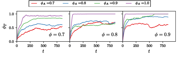
Figure 5: Translational order parameter $\phi_{T}$ as a function of time for different values of $\phi$ and $\phi_{A}$. The purple curve corresponds to the case $\phi_{A}=1$, i.e. no passive particles present. We see that in all other cases the state of collective migration is reached later (longer transient phase) or not reached at all, especially for lower $\phi_{A}$ (red curves). Other parameters are $M_{0}^{A}=100$ and $M_{0}^{B}=70$. The data have been obtained as the average of ten different simulations started with different initial conditions.

We now fix the mobility $M_{0}^{B}=70$ and vary $\phi$ and $\phi_{A}$. We reduce $\phi$ down to $0.7$, a limit for which a state of collective migration would still be reached in an homogeneous active system ($\phi_{A}=1$), as seen from the purple lines in figure 5. For $\phi=0.9$ a state of collective migration is reached for $\phi_{A}=0.9$ but with a longer transient phase than for the homogeneous case (green line in figure 5(c)). For $\phi_{A}=0.8$ we already see a small perturbation from the unit value for $\phi_{T}$ and for $\phi_{A}=0.7$ collective migration is no longer reached. We here observe the accumulation of passive particles in certain regions, see also figure 6(d). This hinders the active particles from following a straight trajectory and thus the formation of collective migration. Things change by reducing the total density to $\phi=0.8$. The state of collective migration is not reached, independent of the value of $\phi_{A}$ (figure 5(b)). However, for high relative density $\phi_{A}=0.9$, green curve in figure 5(b) a new state is formed, where the translational order parameter $\phi_{T}$ is at least locally close to one. This new state is discussed below and can be seen in the snapshots in figures 6(a) and (b). For $\phi=0.7$ (figure 5(a)) a decrease in $\phi_{A}$ leads to a decrease of $\phi_{T}$. In this situation there is enough empty space in the system to allow active particles to change their trajectories when interacting with passive ones. This causes a perturbation that gets bigger as the number of passive particles increase, leading to a decrease of $\phi_{T}$.

A more detailed investigation of the intermediated regime with $\phi=0.8$ and $\phi_{A}=0.9$ is shown in figure 6(a) and (b), showing an intermediate state with two regions of active particles moving in opposite direction. The regions are separated by passive particles. This separation prevents the alignment of the collectively migrating domains. This state can be seen as a local flocking state. It is more stable in figure 6(a), persisting for the whole simulation time, and less stable in figure 6(b), where the alignment of passive particles will be destroyed after a while and a transition to collective migration follows (see supplementary video). However, even if this collective migration state is reached the passive particles are not randomly distributed. As see in figure 6(c) they form chains, which persist over longer periods of time and are transported by the active particles. If the number of passive particles is increased $\phi_{A}=0.7$ a clustering of passive particles within the active bath can be observed, see figure 6(d). These new states and patterns are characteristic for binary mixtures and should be explored further, both numerically and experimentally.

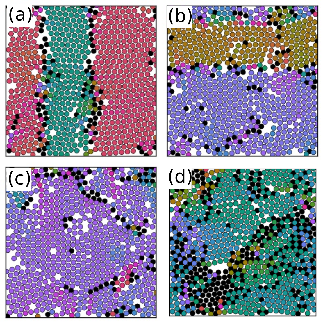
Figure 6: The color code corresponds to the single particle velocity. (a) Snapshot of a state of local flocking, with two macro regions of active particles having exactly opposite orientation. This state can last for a long time thanks to the presence of passive particles at the boundary between the two regions (see also supplementary video). (b) Another state of local flocking. Here, less passive particles are accumulated at the boundary between the moving active regions. The situation is less stable and transforms in a situation of global collective motion (c), in which passive particles form chains, which persist over longer periods of time. (d) Passive particles forming clusters in an active bath. (a) - (c) regime $\phi=0.8$, $\phi_{A}=0.9$, (d) regime $\phi=0.9$, $\phi_{A}=0.7$.

IV Conclusions

In summary, our microscopic field theoretical approach for binary mixtures of interacting active and passive particles has been used to investigate a wide spectrum from dilute systems $\phi<0.7$ to dense systems $\phi>0.7$ with a relatively low fraction of active particles $\phi_{A}<0.2$ (active doping) and a relatively high fraction $\phi_{A}>0.7$ (active bath), respectively. We have demonstrated with one and the same model a variety of known phenomena, such as enhanced crystallization via active doping Kümmel et al. (2015); Ni et al. (2014) and suppressed crystallization in dense systems Kümmel et al. (2015). We also analyzed the limits of collective migration, which for the special case of immobile passive particles qualitatively reproduce the results in Morin et al. (2017b). Within the experiments in Kümmel et al. (2015) and in our simulations the suppression of collective migration sensitively depends on the fraction of immobile passive particles. Within the experimentally less explored state of mobile passive particles we found new phenomena. For fractions of passive particles, for which collective migration is suppressed if the passive particles are immobile, collective motion is still possible if the mobility of these particles is large enough. But there are also intermediate regime, characterized by local flocking states, where regions of active particles are separated by boundary layers of passive ones. We further found chains of passive particles and clusters which persist for a relatively long time. A rigorous classification of these states remains open and should be addressed with experimental investigations.

As already pointed out, the proposed microscopic field theoretical model can easily be modified to consider more than two species, species with different size and interaction potential and active species with different self-propulsion velocities, which makes the approach a generic tool to study active systems in complex environments. Also hydrodynamic interactions have already be considered together with a (passive) phase field crystal model Praetorius and Voigt (2015a); Heinonen et al. (2016) and they could also be included in our model.