Arbitrary-order Hilbert spectral analysis and intermittency in solar wind density fluctuations

Abstract

The properties of inertial and kinetic range solar wind turbulence have been investigated with the arbitrary-order Hilbert spectral analysis method, applied to high-resolution density measurements. Due to the small sample size, and to the presence of strong non-stationary behavior and large-scale structures, the classical structure function analysis may prove to be unsuccessful in detecting the power law behavior in the inertial range, and may underestimate the scaling exponents. However, the Hilbert spectral method provides an optimal estimation of the scaling exponents, which have been found to be close to those for velocity fluctuations in fully developed hydrodynamic turbulence. At smaller scales, below the proton gyroscale, the system loses its intermittent multiscaling properties, and converges to a monofractal process. The resulting scaling exponents, obtained at small scales, are in good agreement with those of classical fractional Brownian motion, indicating a long term memory in the process, and the absence of correlations around the spectral break scale. These results provide important constraints on models of kinetic range turbulence in the solar wind.

94.05.-a, 94.05.Lk, 47.27.-i

1 Introduction

The solar wind is a continuous flow of plasma expanding from the solar corona into interplanetary space. Almost sixty years after the first spacecraft measurements, our knowledge of solar wind phenomena has largely advanced, but many aspects of the fundamental processes are still not understood. Among these, the properties of turbulence and its role in the non-adiabatic expansion of the solar wind is one of the major research goals for the community (Bruno & Carbone, 2013). Power-law spectra of velocity, magnetic field and density fluctuations have long been observed throughout the heliosphere, and represent a robust characteristic of solar wind turbulence (Bruno & Carbone, 2013). Unlike neutral fluid turbulence, the weakly collisional nature of solar wind plasma results in the presence of several scaling ranges. At scales larger than a few hours, the large-scale structure of the solar wind, probably of solar origin, generates a spectral region of energy input which can also display $E(\nu)\sim\nu^{-1}$ scaling (Bruno & Carbone, 2013), where $\nu$ is the spacecraft-frame measured frequency, and is characterized by mostly uncorrelated fluctuations. In the range between a few hours and a few seconds, the solar wind behaves as a magnetized flow and follows similar prescriptions to the classical Kolmogorov inertial range turbulence picture (Kolmogorov, 1941). Various adaptions of the Kolmogorov phenomenology to MHD turbulence have been proposed (Iroshnikov, 1964; Kraichnan, 1965; Goldreich & Sridhar, 1995; Boldyrev, 2006), and the solar wind shows several properties that match these models, although aspects of these are still under debate. At smaller scales, the turbulence coexists with field-particle interactions (He et al., 2015), plasma instabilities, and other kinetic plasma processes. In this range, a steeper power-law spectrum is generally observed, whose nature is still under investigation (Leamon et al., 1998; Alexandrova et al., 2008, 2013; Chen, 2016; Consolini et al., 2017).

Among the turbulence characteristics, inertial range intermittency of velocity and magnetic field has been deeply studied in recent years (Bruno & Carbone, 2013). Data analysis has shown that, as for neutral flows, the energy cascade is inhomogeneous, with the generation of localized small-scale structures which result in scale-dependent, non-Gaussian statistics of the field fluctuations (Marsch & Tu, 1997; Sorriso-Valvo et al., 1999). The appropriate estimation of the degree of intermittency is important for determining the presence of energetic structures, such as vorticity filaments and current sheets, which are likely to play an important role in the dissipative and kinetic processes occurring in the small-scale range (Alexandrova et al., 2013). For example, numerical simulations have shown that magnetic reconnection may occur within current sheets (Servidio et al., 2012), and plasma instabilities are also mostly excited in the presence of these structures (Servidio et al., 2014). On the other hand, the presence of intermittency in the small-scale range is still not fully established, although most magnetic field observations seem to indicate self-similar, non-intermittent scaling in this range (Kiyani et al., 2009). However, different techniques have given different results (Alexandrova et al., 2008). This ambiguity needs to be resolved, for a better constraint on the cascade and dissipative processes.

While most of the literature concerns the magnetic field fluctuations, some works have focused on the properties of density fluctuations. In particular, the turbulence and intermittency properties of density have been studied in the inertial range (Hnat et al., 2003; Bruno et al., 2014; Chen et al., 2011) and, more recently, at smaller scales (Chen et al., 2014; Sorriso-Valvo et al., 2017). The analysis of Spektr-R data have shown the presence of two power-law frequency spectra $E(\nu)\propto\nu^{-\beta}$, separated by a break located around the proton gyro-scale (Šafránková et al., 2013, 2013; Chen et al., 2014; Šafránková et al., 2015). In particular, a scaling typical of the inertial range, characterized by a power-law decay of the spectral density (with a slope $\beta\simeq 5/3$) is found at large scales, and steeper spectra with slopes in the range $\beta\simeq 1.76$–$2.86$ exist at smaller scales (Sorriso-Valvo et al., 2017). In the inertial range, the structure functions do not show proper scaling, so that the deviation from $K41$ (Kolmogorov, 1941) was only evaluated through the standard multifractal analysis on a surrogate dissipation field (Sorriso-Valvo et al., 2017). As in the case of magnetic field, the determination of the presence of intermittency in the kinetic range is ambiguous, as different techniques resulted in different answers (Chen et al., 2014; Sorriso-Valvo et al., 2017). Indeed, the scaling exponents obtained through the structure function analysis suggested a lack of intermittency (Chen et al., 2014), although also showed some variability between intervals. Similar variability was also observed in the multifractal spectrum (Sorriso-Valvo et al., 2017), suggesting that further analysis is required to fully understand the properties of this small scale dynamics. This ambiguity motivates the use of alternative techniques, in order to understand whether or not nonlinear correlations are generated also in this range of scales.

The difficulty in evaluating the presence of intermittency at small scales has several possible causes. First, the limited size of high-resolution samples causes possible effects due to poor statistical convergence, stationarity or ergodicity. Second, the role of the inertial-range fluctuations may affect the statistical assessment of small-scale turbulence, because the presence of larger-scale strucures (often in the form of ramp-cliff structures as also observed in solar wind density, see for example the top panel of Figure 7) may lead, for example, to underestimation of the spectral index and of the structure function scaling exponents. Ramp-cliff structures are a common features of scalar turbulence (Shraiman, 2000; Warhaft, 2000), and have been observed in a variety of turbulent shear flows in both stably and unstably stratified conditions (Wroblewski et al., 2007). The typical pattern can be identified by a very rapid increase of the field (cliff), followed by a more gradual, or smooth decrease (ramp), or in reverse order (Sreenivasan, 1991; Celani et al., 2000; Wroblewski et al., 2007). It is believed that the large scale structures may non-locally couple with the small scales through the cliff structure (Yeung et al., 1995). Furthermore, it has been shown that even the inertial range scaling may be affected by the presence of large-scale periodic forcing structures (Huang et al., 2010). This may have strong influence on both the small-scale and large-scale statistics (Huang et al., 2011, 2010). Ramp-cliff structures cannot be represented by a simple monochromatic component, and Fourier-based methods require high-order harmonic components to represent their difference. This lead to an asymptotic approximation process (Cohen, 1995; Huang et al., 1998; Flandrin, 1999), resulting in an artificial energy flux from large to the small scales (Huang et al., 2011). As a result the Fourier-based power spectrum is contaminated by this artificial energy flux, which is manifested as a shallower power spectrum (Huang et al., 2010). All these effects may be particularly important when the sample size is limited.

To correctly extract scaling information for solar wind proton density fluctuations, by minimizing the effect of the non-stationarity and the ramp-cliff structures embedded in the field, arbitrary-order Hilbert Spectral Analysis (HSA) (Huang et al., 2008, 2010; Carbone et al., 2016a) has been used in this work. HSA formally represents an extension of classical Empirical Mode Decomposition (EMD), designed to characterize scale invariant properties directly in amplitude-frequency space (Huang et al., 2008). EMD was developed to process and analyze the temporal evolution of nonstationary data (Huang et al., 1998) and has been used in many different fields (Salisbury & Wimbush, 2002; Vecchio et al., 2014; Carbone et al., 2016b; Alberti et al., 2017), including the analysis of fast, quasi-stationary solar wind high-resolution magnetic field data, as measured by the Cluster spacecraft (Consolini et al., 2017). The main advantage of EMD is that the basis functions are derived from the signal itself. Since EMD analysis is adaptive (in contrast to traditional decomposition methods where the basis functions are fixed) and not restricted to stationary data, the data set may be analyzed without introducing spurious harmonics or artifacts near sharp data transitions, which could appear when using classical Fourier filtering or high order moments analysis. Indeed, EMD allows local information to be extracted through the instantaneous frequencies which cannot be captured by fixed-frequency methods (like Fourier or Wavelets). The main consequence is that the frequency is not widely spread (as for Wavelets), with a much better frequency definition and smaller amplitude-variation-induced frequency modulation (Huang et al., 1998; Liu et al., 2012).

2 Arbitrary order Hilbert spectral analysis of solar wind proton density data

In order to perform the arbitrary-order Hilbert Analysis, the high-resolution solar wind proton density $n_{p}$ (with a sampling rate $\Delta t=0.031$ sec), measured by the BMSW instrument (Šafránková et al., 2013) on the Spektr-R spacecraft, have been used (Šafránková et al., 2013, 2013; Chen et al., 2014; Šafránková et al., 2015; Sorriso-Valvo et al., 2017). All of the intervals were collected during the period November 2011 to August 2012, and the total length of each interval is between 1 and 4 hours. In addition, the proton velocity $v_{p}$ and temperature $T_{p}$ were also sampled at the same frequency. The magnetic field $B$, not provided by Spektr-R instrumentation, was supplied by MFI on the Wind spacecraft, in the corresponding time interval (Chen et al., 2014), and was only used for estimating the typical plasma beta $\beta_{p}$ of the intervals. All of the parameters are collected in Table 1. More details about the data can be found in (Sorriso-Valvo et al., 2017). As customary, the Taylor hypothesis is used to shift between time and space variables via the bulk solar wind speed, which is supersonic and super-Alfvénic for all intervals. In these conditions, the time series will be used as an instantaneous one-dimensional cut into the turbulent flow, so that all of the arguments in terms of space and wavevector will be given in terms of time and frequency, without loss of generality.

Table 1: Main parameters for the eight intervals. Data are from Spektr-R, except $B$, which is from the upstream Wind spacecraft. The Date (dd/mm/yyyy) refers to the initial time of the measurement. Time is in UT, magnetic field $B$ in nT, the proton density $n_{p}$ in cm^-3, and the proton speed $v_{p}$ in km s^-1.

Interval	Date	Time	$\beta_{p}$	$B$	$n_{p}$	$v_{p}$
$A$	10/11/2011	15:55:40–18:46:55	0.78	4.7	4.6	370
$B$	01/06/2012	21:05:44–01:09:06	0.12	8.3	6.6	370
$C$	02/06/2012	02:34:52–03:26:43	0.17	9.1	7.9	360
$D$	02/06/2012	06:02:22–08:07:15	0.18	8.8	8.2	330
$E$	09/07/2012	08:25:56–11:09:51	0.06	12.0	6.0	400
$F$	09/07/2012	13:22:18–16:55:40	0.14	11.0	6.7	390
$G$	09/08/2012	10:48:52–15:59:13	0.74	4.7	4.0	320
$H$	09/08/2012	17:40:39–22:31:50	0.41	4.5	6.3	330

To apply HSA, the solar wind density measurements $n_{p}(t)$ were initially decomposed through classical EMD to obtain the intrinsic mode functions (IMFs), and the Hilbert transform was then applied to the IMFs. Within the EMD framework, the data are decomposed into a finite number $k$ of oscillating basis functions $\phi_{j}(t)$, known as intrinsic mode functions (IMFs), characterized by an increasing time scale $\tau$, and a residual $r_{k}(t)$ which describes the mean trend, if one exists, as

$$n_{p}(t)=\sum_{j=1}^{k}\phi_{j}(t)+r_{k}(t)\,.$$ (1)

The decomposition includes two stages: first, the local extrema of $n_{p}(t)$ are identified and subsequently connected through cubic spline interpolation. Once connected, the envelopes of local maxima and minima are obtained. Second, the mean $M_{1}(t)$ is calculated between the two envelope functions, then subtracted from the original data, $h_{1}(t)=n_{p}(t)-M_{1}(t)$. The difference $h_{1}(t)$ is an IMF only if it satisfies the following criteria: (i) the number of local extrema and zero crossings does not differ by more than 1; (ii) at any point $t$, the mean value of the extrema envelopes is zero. When $h_{1}(t)$ does not meet the above criteria, the sifting procedure is repeated using $h_{1}(t)$ as the new raw data series, and $h_{11}(t)=h_{1}(t)-M_{11}(t)$ is generated, where $M_{11}$ (t) is the mean of the envelopes. The sifting procedure is repeated $m$ times until $h_{1m}(t)$ satisfies the above criteria. A general rule to stop the sifting is introduced by using a standard deviation $\sigma$, evaluated from two consecutive steps:

$$\sigma=\sum_{t=0}^{N}\frac{|h_{1(m-1)}(t)-h_{1m}(t)|^{2}}{h_{1(m-1)}^{2}(t)}\,.$$ (2)

The iterative process stops when $\sigma$ is smaller than a threshold value $\sigma_{\mathrm{thresh}}$ (Huang et al., 1998; Cummings et al., 2004).

Since EMD acts intrinsically as a dyadic filter bank (Flandrin et al., 2004; Huang & Shen, 2005), each IMF captures a narrow spectral band in frequency space (Huang et al., 2008, 2010; Carbone et al., 2016a) and their superposition behaves as $M(\nu)\equiv\text{Max}[\phi_{j}(\nu)]\sim\nu^{-\alpha}$. In Figure 1, the results of the EMD performed on interval A are reported. In both ranges, the behavior of $M(\nu)$ is compatible with the Fourier spectral indexes: $\alpha\approx 1.66$ and $\alpha\approx 2.6$, for the inertial range and below the proton gyroscale respectively.

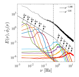
Figure 1: Comparison of Fourier power spectral density $E(\nu)$ (black line) for interval A with the Fourier power spectrum of the different IMFs extracted from the EMD $\hat{\phi}(\nu)$, as a function of frequency $\nu$. The band like structure of each $\hat{\phi}(\nu)$ shows the dyadic nature of the decomposition. The solid black line indicates $M(\nu)\sim\nu^{-1.66}$ for the inertial range, while the dot-dashed line indicates $M(\nu)\sim\nu^{-2.6}$ for the scales below the proton gyroscale. The vertical dashed line indicates the position of the proton gyroscale. The gyroscale is the frequency corresponding (via the Taylor hypothesis) to $k\rho_{i}=1$, $\rho_{i}$ being the proton gyroradius.

By comparison with the Fourier spectrum, each IMF can be interpreted according to its characteristic time scale. In particular, as visible in Figure 1, modes 11 to 16 capture the dynamics of the MHD inertial range, while modes 2 to 6 capture the small scale dynamics below the proton gyroscale. The intermediate range of scales, modes 7 to 10, do not show power-law scaling, and are representative of the dynamics across the break scale, where the Fourier spectrum is not described by a power-law. Finally, mode $\phi_{1}(t)$, associated to the smallest time scale, captures the experimental noise embedded in the datasets (Wu & Huang, 2004; Cummings et al., 2004), setting the upper limit of the resolvable dynamics and breaking the spectral power-law decay. It is worth mentioning that larger scale modes with $n>16$ also exist and are nonvanishing. In particular, modes 17 to 20 do not present any particular scaling, and can be associated with large-scale structures that could act as an energy source for the inertial range.

Once the IMFs have been obtained, the next step of our analysis is to compute the Hilbert transform of each mode

$$\phi_{j}^{\star}=\frac{p}{\pi}\int_{-\infty}^{+\infty}\frac{\phi_{j}(\tau)}{t-\tau}d\tau\,,$$ (3)

where $p$ is the Cauchy principal value and $\phi_{j}(t)$ is the $j$-th IMF. The combination of $\phi_{j}(t)$ and $\phi_{j}^{\star}(t)$ defines the analytical signal $\mathcal{Z}=\phi_{j}+i\phi_{j}^{\star}=\mathcal{A}_{j}(t)e^{i{\theta(t)}}$, where $\mathcal{A}_{j}(t)$ is the time-dependent amplitude modulation and $\theta(t)$ is the phase of the mode oscillation (Cohen, 1995).

For each mode, the Hilbert spectrum, defined as $H(\nu,t)=\mathcal{A}^{2}(\nu,t)$ (where $\nu=d\theta/dt$ is the instantaneous frequency), provides energy information in the time-frequency domain. A marginal integration of $H(\nu,t)$ provides the Hilbert marginal spectrum $h(\nu)=T^{-1}\int_{0}^{T}H(\nu,t)dt$, defined as the energy density at frequency $\nu$ (Huang et al., 1998, 1999). In addition, from the Hilbert spectrum, a joint probability density function $P(\nu,\mathcal{A})$ can be extracted, using the instantaneous frequency $\nu_{j}$ and the amplitude $\mathcal{A}_{j}$ of the $j$-th IMF. This allows the Hilbert marginal spectrum $h(\nu)$ to be written as

$$h(\nu)=\int_{0}^{\infty}P(\nu,\mathcal{A})\mathcal{A}^{2}d\mathcal{A}\,,$$ (4)

which corresponds to a second order statistical moment (Huang et al., 2008). Equation 4 can be generalized to the arbitrary order $q\geq 0$ by defining the $\nu$-dependent $q$th-order statistical moments

$$\mathcal{L}_{q}=\int_{0}^{\infty}P(\nu,\mathcal{A})\mathcal{A}^{q}d\mathcal{A}\,,$$ (5)

In particular, it can be shown that $h(\nu)=\mathcal{L}_{2}$ represents the analogue of the Fourier spectral energy density (Huang et al., 2008).

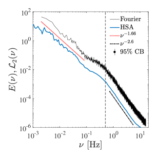
Figure 2: Comparison of Fourier power spectrum (thin line) with $\mathcal{L}_{2}(\nu)$ (thick line) for proton density data (interval A). Both methods show a power-law behavior in the inertial range and in the small-scale range, with a slope $\beta\approx 1.66$ and $\beta\approx 2.66$ respectively. The vertical dashed line represents the proton gyroscale. The curves have been vertically shifted for clarity.

In Figure 2, the classical power spectral density $E(\nu)$ evaluated through the Fourier transform is compared with the associated $\mathcal{L}_{2}(\nu)$, obtained through the HSA. Again, the power-law behavior is present in the same two ranges (i.e. $\mathcal{L}_{2}(\nu)\sim\nu^{-\beta}$), and the slope $\beta$ is compatible with the Fourier spectrum: for $\mathcal{L}_{2}$, power-law fits give $\beta=1.66\pm 0.05$ for the inertial range and $\beta=2.60\pm 0.01$ for the small-scale range. A better scaling of $\mathcal{L}_{2}$ can be observed at large scales, where the traditional Fourier spectral density shows a weak amplitude modulation, in the frequency range $\nu\in[10^{-2},10^{-1}]$ Hz, comparable with the typical observed size of the ramp-cliff structures (see Figure 7 top panel) (Huang et al., 2010; Carbone et al., 2016a). By analyzing the data, the ramp-cliff duration $T$ has been found in the range $T\in[35\pm 13,300\pm 39]$ sec, with an average duration of the order of $71.4$ sec for the ramps and $27.2$ sec for the cliffs.

Thanks to the local nature of EMD and HSA, these sources of modulation, as well as the possible effects of ramp-cliff structures, can be constrained, isolating the properties of the cascade from the possible effects of the larger scale forcing and residual structures (Huang et al., 2010). The scaling properties of the small-scale fluctuations can thus be studied independently of the effect of the intermittent structures arising in the inertial range. Similarly, the inertial range scaling can be studied independently of the effect of of the uncorrelated large-scale fluctuations, often observed as a $\nu^{-1}$ spectral range (Bruno & Carbone, 2013). Due to this local nature, HSA allows a better determination of the spectral scaling exponents by mitigating the effects of the instrumental noise and of the larger-scale energy inhomogeneity, both in the inertial range and in the small-scale range. An exhaustive comparison of the results obtained through HSA, detrended fluctuation analysis (DFA), structure functions (SF) and wavelet transforms (WT) has been performed in (Huang et al., 2011). It was found that both the DFA and WT methods underestimate the scaling exponents, while the SF method may be affected by the presence of ramp-cliff structures or large scale periodic forcing (Huang et al., 2010; Carbone et al., 2016a).

3 Intermittency Results

As described in Section 2, the generalized second-order Hilbert spectrum has two ranges of power-law scaling $\mathcal{L}_{2}\sim\nu^{-\beta}$. In the current Spektr-R density data $n_{p}(t)$, it is possible to extend the measurement of the scaling properties of $\mathcal{L}_{q}(\nu)$ up to the $5$-th order. Figure 3 shows $\mathcal{L}_{q}(\nu)$ for orders $q=1,\dots,5$, obtained from Eq. 5 using interval A. The resulting $\mathcal{L}_{q}(\nu)$ show clear scaling behavior $\mathcal{L}_{q}(\nu)\sim\nu^{-\beta_{q}}$ for all $q$, in the two frequency ranges where the spectra behave as power laws.

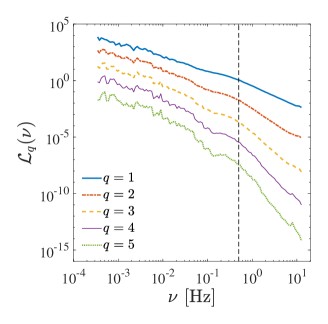
Figure 3: The Hilbert spectra $\mathcal{L}_{q}(\nu)$ for $q=1,\dots,5$, obtained for interval A. The generalized spectra have been shifted for clarity. The dashed line represents the proton gyroscale.

Classically, the spectral exponent $\beta$ is linked to the scaling exponent of the second order structure function $S(2)\equiv\langle|x(t+\tau)-x(t)|^{2}\rangle\sim\tau^{\zeta(2)}$ (for a generic field, of component $x(t)$) via the relation $E(\nu)\sim\nu^{-\beta}\to\beta=1+\zeta(2)$. Extending this relationship to any arbitrary order $q$, a family of generalized scaling exponents $\xi(q)$ can be introduced through the generalized Hilbert spectra (Huang et al., 2010; Carbone et al., 2016a) as $\xi(q)\equiv\beta_{q}-1$. The exponents $\xi(q)$ are the Hilbert analogous of the standard scaling exponents $\zeta(q)$ obtained through the structure functions or through the Extended Self-Similarity (ESS) (Benzi et al., 1993; Arneodo et al., 1996). Equation (5) therefore is an alternative to the structure function scaling exponents to quantitatively estimate the level of intermittency in the turbulent cascade (Frisch, 1995), with the advantage of constraining the effects of noise and large-scale structure. The scaling exponents $\xi(q)$ for the inertial range obtained from the generalized Hilbert spectra $\mathcal{L}_{q}(\nu)$ are shown in Figure 4. The range of $\nu$ selected in order to evaluate the scaling exponent $\xi(q)$ lies in the closed interval $\nu\in\left[10^{-3},9\times 10^{-2}\right]$ Hz. Intervals D and G were excluded from the analysis performed in the inertial range, as their limited size does not allow statistical convergence of the high order moments ($q>3$). The same figure shows a comparison of $\xi(q)$ with the classical exponents $\zeta(q)$ measured using Extended Self-Similarity (ESS) for the Eulerian velocity fluctuations in fully developed hydrodynamic turbulence experiments (Benzi et al., 1993; Arneodo et al., 1996). It is easily observed that the departure from the $K41$ scaling is captured in the solar wind density data, and that the exponents $\xi(q)$ are similar to the standard $\zeta(q)$ obtained in Navier-Stokes fully developed turbulence through the ESS. These are shown as reference, as neither structure functions nor the ESS analysis provided power-law scaling for the solar wind density in this range (Chen et al., 2014).

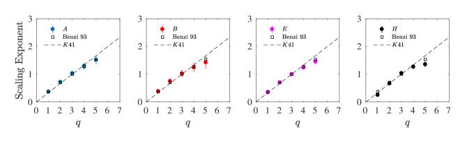
Figure 4: Scaling exponents $\xi(q)$ obtained through the HSA, in the inertial range, for solar wind density in the intervals A, B, E, H (solid symbols); exponents $\zeta(q)$ obtained from velocity fluctuations measured in the inertial range of hydrodynamic turbulence using ESS (open symbols) (Benzi et al., 1993; Arneodo et al., 1996), shown as reference; dashed line: theoretical expectation $q=1/3$, as estimated from dimensional analysis in the absence of intermittency (Kolmogorov, 1941).

The same analysis has been performed on the small-scale range, below the proton gyroscale, in the range $\nu\in\left[1.5,9.8\right]$ Hz. The scaling exponents $\xi(q)$ extracted from the generalized Hilbert spectra $\mathcal{L}_{q}(\nu)$ are shown in Figure 5. The results are different from the inertial range; in particular, monofractal behavior is found, with $\xi(q)$ presenting a linear scaling compatible with $\xi(q)\sim 4/5q$ for intervals A, B, C, D, G, H, and $\xi(q)\sim 3/5q$ for intervals E, F. As a comparison, in Figure 5, the scaling exponents $\zeta(q)$ obtained through the structure function (Chen et al., 2014) in a similar range of scales are reported (the ESS analysis performed in this range gives identical results that are not shown for clarity). The difference between the two exponent sets is evident.

The weak curvature of $\zeta(q)$ could be the remnant signature of the inertial range structure, which acts as forcing for the dynamics in this range. The EMD-HSA analysis helps to remove these large-scale effects  (Huang et al., 2010), to reveal the non-intermittent nature of the small-scale density fluctuations in the solar wind. This result is in contrast with the recent multifractal analysis of the same data (Sorriso-Valvo et al., 2017), where the traditional box-counting measure applied to a surrogate dissipation field suggested a high level of multifractality in the small-scale range. However, the HSA analysis reveals the monofractal nature of the fluctuations, suggesting that the apparent multifractal properties may be the result of residual larger scale structure (inertial range). A similar monofractal behavior has been found in Consolini et al. (2017) (with different Hurst numbers $\mathcal{H}$), where the linear scaling has been obtained by analyzing the high-resolution Cluster magnetic field dataset at kinetic scales, and for each magnetic field component.

In order to further check the absence of intermittency, we compare the scaling exponents obtained from $n_{p}(t)$ with the exponents obtained from the HSA applied to fractional Brownian motion (fBm), with characteristic Hurst number $\mathcal{H}=4/5$ and $\mathcal{H}=3/5$, respectively. The Hurst number $\mathcal{H}$ describes the long-term memory (persistence) of a process, or the influence “past” increments have on “future” ones. Values in the range $\mathcal{H}\in(0.5,1]$ indicate a persistent (long-term memory, correlated) process, while values $\mathcal{H}\in[0,0.5)$ are associated with anti-persistent (short-term memory, anti-correlated) processes. $\mathcal{H}=0.5$ indicates a completely uncorrelated process (e.g., a random walk). In the classical Kolmogorov theory, in the absence of intermittent corrections, $\zeta(q)=q\mathcal{H}$. By exploiting the relation $\xi(q)=\beta_{q}-1\propto\zeta(q)$ we expect $\xi(q)+1\equiv q\mathcal{H}+1$. The comparison between $\xi(q)$ and the scaling exponents for the fBm ($\mathcal{H}=4/5$) is given in Figure 6, which shows an excellent agreement supporting the absence of intermittency.

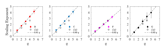
Figure 5: Scaling exponents $\xi(q)$ of the solar wind density, extracted from intervals B, C, F, G (full symbols) at small scale. The dashed lines represent the fitted linear scaling $\xi(q)\simeq 4/5q$ for intervals B, C, G, and $\xi(q)\simeq 3/5q$ for interval F. The open symbols represent the solar wind density scaling exponents $\zeta(q)$ evaluated through the standard Kolmogorov structure functions (Chen et al., 2014).

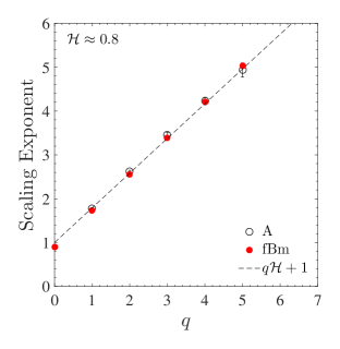
Figure 6: Scaling exponents $\xi(q)+1$ extracted from interval A (open symbols), and for fractional Brownian motion simulation with Hurst number $\mathcal{H}=4/5$. The dashed line represents the theoretical scaling $q\mathcal{H}+1$.

The local Hurst number has been also estimated using an alternative method. The evaluation of local Hurst exponent is a nontrivial issue, for which different approaches have been proposed in the past years. One of the most accurate, fast and simple methods for nonstandard, Gaussian, multi-fractional Brownian motion is the Detrending Moving Average (DMA) technique (Alessio et al., 2002; Carbone et al., 2004; Consolini et al., 2013). Despite its simplicity, this method, based on the analysis of the scaling features of the local standard deviation around a moving average, is more accurate than other methods. The DMA technique consists of evaluating the scaling features of the quantity:

$$\sigma_{\mathrm{DMA}}^{2}(n)={\frac{1}{N_{\mathrm{max}}-n}\sum_{j=n}^{N_{\mathrm{max}}}\left[f(t)-\bar{f}_{n}(t)\right]^{2}}\,,$$ (6)

where $\bar{f}_{n}(t)$ represents the average on a moving time window of length $n$, for different values of the time window in the interval $t_{w}\in[n,N_{\mathrm{max}}]$. By applying this procedure, the quantity $\sigma_{n}(t)$ is expected to behave as $\sigma_{n}(t)\sim n^{\mathcal{H}}$. In order to evaluate $\sigma_{n}(t)$ from the solar wind proton density time series, a moving window of approximately $N_{\mathrm{max}}=155$ s has been selected.

The detailed temporal evolution of the small-scale $\mathcal{H}_{l}(t)$ is shown in Figure 7. The top panel shows the density profile $n_{p}(t)$ for interval A, and the lower panel shows the temporal evolution of the local Hurst number. The results are in good agreement with the Hurst number extracted through the HSA, in particular a value $\mathcal{H}\approx 0.83\pm 0.03$ has been found. The maximum percentage error with respect to the empirical value $\mathcal{H}=0.8$ is of the order of $\Delta\mathcal{H}=7\%$. The results relative to the other intervals are reported in Table 2

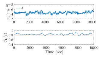
Figure 7: Top panel: the solar wind proton density for interval A. The presence of ramp-cliff structures is visible, for example for Time between 4000 and 5000 sec. Bottom panel: temporal evolution of the local Hurst number $\mathcal{H}_{l}(t)$ evaluated through the DMA method (bottom panel), for interval A. The horizontal dashed line represents the expected value $\mathcal{H}_{l}=4/5$.

An example of $\sigma_{\mathrm{DMA}}(n)$, obtained from interval A at $t=6$ s, is given in Figure 8. At small scales $n\in[0.1,0.6]$ s, $\sigma_{\mathrm{DMA}}(n)$ shows a good power-law scaling which provides $\mathcal{H}\approx 4/5$, in good agreement with HSA results. The small-scale power-law behaviour was robustly observed for all time windows $t_{w}$, in all intervals. A second power-law range is also always found in the intermediate range of scales $n\in[1,3]$ s, around the spectral break scale, where $\mathcal{L}_{2}(\nu)$ does not show power-law scaling.

Table 2: For all intervals (first column): the empirical estimate of the Hurst exponent $\mathcal{H}$ for the scaling exponents $\xi(q)$ extracted through HSA (second column); the average $\langle\mathcal{H}_{l}(t)\rangle$ (third column) and the standard deviation $\sigma_{\langle\mathcal{H}\rangle}$ (fourth column) of the Local Hurst number evaluated through the DMA method; and the maximum percentage error $\Delta\mathcal{H}\%$ with respect to the empirical value $\mathcal{H}$.

Interval	$\mathcal{H}$	$\langle\mathcal{H}_{l}(t)\rangle$	$\sigma_{\langle\mathcal{H}\rangle}$	$\Delta\mathcal{H}\%$
$A$	$0.8$	$0.84$	$0.03$	$7.0$
$B$	$0.8$	$0.79$	$0.05$	$5.2$
$C$	$0.8$	$0.77$	$0.06$	$7.4$
$D$	$0.8$	$0.85$	$0.05$	$7.4$
$E$	$0.6$	$0.57$	$0.09$	$12.0$
$F$	$0.6$	$0.61$	$0.09$	$12.0$
$G$	$0.8$	$0.72$	$0.06$	$9.8$
$H$	$0.8$	$0.82$	$0.07$	$5.4$

It is interesting to observe that in this range the typical exponent for random processes $\mathcal{H}_{l}\approx 1/2$ is found, exposing the uncorrelated nature of the phenomenon during the transition between the two ranges of scales. For example, some mechanisms could act to decorrelate the intermittent field at the end of the inertial range cascade, subsequently injecting energy inhomogeneously in the small-scale range. The possibility of understanding the nature of the transition region dynamics using HSA analysis is an important issue that will be studied in depth in a dedicated work. Finally, in the inertial range ($n>5$ s) there is no evidence of single power-law scaling, in agreement with the multifractal dynamics in this range.

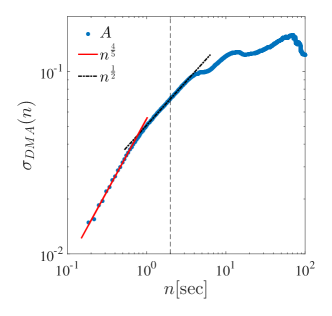
Figure 8: Local Hurst number evaluated through the DMA method. Full symbols: $\sigma_{DMA}(n)$ as a function of the window length $n$. Thick red line: range of scales $n$ used to retrieve the small scale Hurst number $\mathcal{H}_{l}$. The scaling is in good agreement with the Hurst number evaluated through the HSA. Dot-dashed line: the secondary range across the proton gyroscale. Vertical dashed line: the proton temporal gyroscale.

After averaging over all running windows, the mean Hurst exponents $\langle\mathcal{H}_{l}(t)\rangle$ are obtained for each interval. The results are compatible with the fit of the scaling exponents $\xi(q)$, as visible in Figure 9 where the two sets of values are plotted for the different intervals. Notice that for the HSA exponents the values are consistently closer to the mean values $\mathcal{H}=4/5$ (and $\mathcal{H}=3/5$ for intervals E and F). The small discrepancy between the two techniques could be attributed to the larger-scale structure, which introduces non-stationarity effects and artificial fluctuations in the scaling exponents, which may mimic multifractality (Sorriso-Valvo et al., 2017). Such effects are removed by HSA, so that the associated local Hurst $\mathcal{H}_{l}(t)$ values are less affected by the large-scale fluctuations.

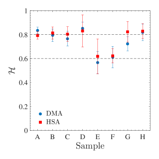
Figure 9: Hurst number $\mathcal{H}$, evaluated through HSA (red squares, the error bars representing the fit parameter uncertainty) and through DMA (blue circles, the error being the standard deviation $\sigma_{\langle\mathcal{H}\rangle}$ from Table 2). The horizontal dashed lines indicate the empirical values $\mathcal{H}=4/5$ and $\mathcal{H}=3/5$.

4 Conclusions

In an attempt to describe the statistical properties of small-scale turbulence in the solar wind, the Empirical Mode Decomposition and the associated arbitrary-order Hilbert Spectral Analysis techniques have been applied for the first time to high-frequency density measurements from the Spektr-R spacecraft. By constructing a family of generalized Hilbert spectra $\mathcal{L}_{q}(\nu)$, the analogous of the scaling exponents of the structure functions have been evaluated from the data. The dyadic filter nature of EMD limits the effects of the large-scale structure (Flandrin et al., 2004; Huang et al., 2010; Carbone et al., 2016a), allowing the identification of a scaling range corresponding to the typical inertial range of solar wind turbulence. Such a scaling range was not observed in this particular dataset using the traditional higher-order moments of the fluctuations. The exponents $\xi(q)$ estimated through HSA fully capture the anomalous scaling properties related to intermittency, exposing the multifractal nature of the inertial range turbulent cascade (Frisch, 1995). In particular, they are found to be in good agreement with the classical exponents observed in Eulerian velocity fluctuations in isotropic fluid turbulence (Benzi et al., 1993; Arneodo et al., 1996).

The high resolution of the Spektr-R density measurements also allows the scaling properties of fluctuations below the proton gyroscale to be investigated, where the presence of intermittency is still debated (Alexandrova et al., 2013; Chen et al., 2014; Sorriso-Valvo et al., 2017). In this range, the scaling exponents obtained through HSA show a linear dependence on the order $\xi(q)\sim q\mathcal{H}$. This suggests that the system loses its multi-scaling properties, and converges to a non-intermittent, mono-fractal behavior. Two values of the Hurst number $\mathcal{H}\approx 3/5,\;4/5$ have been found in the eight intervals under study, indicating a persistent process (long-term memory). The mono-fractal nature of the small-scale fluctuations has been confirmed through a comparison with the HSA analysis of fractional Brownian motion with the same Hurst number. Furthermore, the Hurst number has also been estimated for all intervals using the Detrending Moving Average method. The values obtained with DMA are in good agreement with the HSA results, supporting the validity of the results.

The origin of difference between the intermittency properties of the inertial and kinetic range turbulence in the solar wind, also suggested in some previous works (Kiyani et al., 2009; Chen et al., 2014), remains an important unanswered question. The results in this paper confirm this difference, providing a more accurate measure of the scaling exponents and placing a tighter constraint on the statistical properties of the density fluctuations. Possible reasons for the difference include the increasing importance of wave-particle interactions in the kinetic range, or an inherent difference in the form of the nonlinear interactions of the cascade. The current measurements provide an important constraint on future models of kinetic turbulence.

The results presented in this paper show that the scaling properties of solar wind fluctuations need a careful analysis, and that the larger scale fluctuations may affect the statistical properties of the scales under study. The HSA analysis seems to be able to reduce such effect, providing a more accurate measure of the scaling properties of the field.

References

- Alberti et al. (2017) Alberti, T., Consolini, G., Lepreti, F., et al. 2017, Journal of Geophysical Research: Space Physics, 122, 4266
- Alessio et al. (2002) Alessio, E., Carbone, A., Castelli, G., & Frappietro, V. 2002, The European Physical Journal B - Condensed Matter and Complex Systems, 27, 197
- Alexandrova et al. (2008) Alexandrova, O., Carbone, V., Veltri, P., & Sorriso-Valvo, L. 2008, The Astrophysical Journal, 674, 1153
- Alexandrova et al. (2013) Alexandrova, O., Chen, C. H. K., Sorriso-Valvo, L., Horbury, T. S., & Bale, S. D. 2013, Space Sci. Rev., 178, 101
- Arneodo et al. (1996) Arneodo, A., Baudet, C., Belin, F., et al. 1996, EPL (Europhysics Letters), 34
- Benzi et al. (1993) Benzi, R., Ciliberto, S., Tripiccione, R., et al. 1993, Phys. Rev. E, 48, R29
- Boldyrev (2006) Boldyrev, S. 2006, Phys. Rev. Lett., 96, 115002
- Bruno & Carbone (2013) Bruno, R., & Carbone, V. 2013, Living Reviews in Solar Physics, 10, 2. http://dx.doi.org/10.12942/lrsp-2013-2
- Bruno et al. (2014) Bruno, R., Telloni, D., Primavera, L., et al. 2014, The Astrophysical Journal, 786, 53
- Carbone et al. (2004) Carbone, A., Castelli, G., & Stanley, H. 2004, Physica A: Statistical Mechanics and its Applications, 344, 267
- Carbone et al. (2016a) Carbone, F., Gencarelli, C. N., & Hedgecock, I. M. 2016a, Phys. Rev. E, 94, 063101
- Carbone et al. (2016b) Carbone, F., Landis, M. S., Gencarelli, C. N., et al. 2016b, Geophysical Research Letters, 43, 7751, 2016GL069252
- Celani et al. (2000) Celani, A., Lanotte, A., Mazzino, A., & Vergassola, M. 2000, Phys. Rev. Lett., 84, 2385
- Chen (2016) Chen, C. H. K. 2016, Journal of Plasma Physics, 82, 535820602
- Chen et al. (2011) Chen, C. H. K., Bale, S. D., Salem, C., & Mozer, F. S. 2011, The Astrophysical Journal Letters, 737, L41
- Chen et al. (2014) Chen, C. H. K., Sorriso-Valvo, L., Šafránková, J., & Němeček, Z. 2014, The Astrophysical Journal Letters, 789, L8
- Cohen (1995) Cohen, L. 1995, Time-frequency analysis (Prentice Hall PTR Englewood Cliffs, N.J, 1995)
- Consolini et al. (2017) Consolini, G., Alberti, T., Yordanova, E., Marcucci, M. F., & Echim, M. 2017, Journal of Physics: Conference Series, 900, 012003
- Consolini et al. (2013) Consolini, G., De Marco, R., & De Michelis, P. 2013, Nonlinear Processes in Geophysics, 20, 455
- Cummings et al. (2004) Cummings, D. A., Irizarry, R. A., Huang, N. E., et al. 2004, Nature, 427, 344
- Flandrin (1999) Flandrin, P. 1999, Time-Frequency/Time-Scale Analysis, 1st edn., Wavelet Analysis and Its Applications 10 (Academic Press)
- Flandrin et al. (2004) Flandrin, P., Rilling, G., & Goncalves, P. 2004, IEEE Signal Processing Letters, 11, 112
- Frisch (1995) Frisch, U., ed. 1995, Turbulence: the legacy of A. N. Kolmogorov (Cambridge Univ. Press, Cambridge UK)
- Goldreich & Sridhar (1995) Goldreich, P., & Sridhar, S. 1995, ApJ, 438, 763
- He et al. (2015) He, J., Wang, L., Tu, C., Marsch, E., & Zong, Q. 2015, The Astrophysical Journal Letters, 800, L31
- Hnat et al. (2003) Hnat, B., Chapman, S. C., & Rowlands, G. 2003, Phys. Rev. E, 67, 056404
- Huang & Shen (2005) Huang, N. E., & Shen, S. S. P., eds. 2005, The Hilbert-Huang Transform and Its Applications (World Scientific, Singapore)
- Huang et al. (1999) Huang, N. E., Shen, Z., & Long, S. R. 1999, Annual Review of Fluid Mechanics, 31
- Huang et al. (1998) Huang, N. E., Shen, Z., Long, S. R., et al. 1998, Proceedings of the Royal Society of London A: Mathematical, Physical and Engineering Sciences, 454, 903
- Huang et al. (2011) Huang, Y. X., Schmitt, F. G., Hermand, J.-P., et al. 2011, Phys. Rev. E, 84, 016208
- Huang et al. (2010) Huang, Y. X., Schmitt, F. G., Lu, Z. M., et al. 2010, Phys. Rev. E, 82, 026319
- Huang et al. (2008) Huang, Y. X., Schmitt, F. G., Lu, Z. M., & Liu, Y. L. 2008, EPL (Europhysics Letters), 84, 40010
- Iroshnikov (1964) Iroshnikov, P. S. 1964, Soviet Astron., 7, 566
- Kiyani et al. (2009) Kiyani, K. H., Chapman, S. C., Khotyaintsev, Y. V., Dunlop, M. W., & Sahraoui, F. 2009, Phys. Rev. Lett., 103, 075006
- Kolmogorov (1941) Kolmogorov, A. N. 1941, C. R. Acad. Sci. U.R.S.S, 36, 301
- Kraichnan (1965) Kraichnan, R. H. 1965, Phys. Fluids, 8, 1385
- Leamon et al. (1998) Leamon, R. J., Smith, C. W., Ness, N. F., Matthaeus, W. H., & Wong, H. K. 1998, Journal of Geophysical Research: Space Physics, 103, 4775
- Liu et al. (2012) Liu, Q., Fujita, T., Watanabe, M., & Mitani, Y. 2012, IFAC Proceedings Volumes, 45, 144 , 8th Power Plant and Power System Control Symposium
- Marsch & Tu (1997) Marsch, E., & Tu, C.-Y. 1997, Nonlinear Processes in Geophysics, 4, 101
- Šafránková et al. (2013) Šafránková, J., Němeček, Z., Přech, L., et al. 2013, Space Science Reviews, 175, 165
- Salisbury & Wimbush (2002) Salisbury, J. I., & Wimbush, M. 2002, Nonlinear Processes in Geophysics, 9, 341
- Servidio et al. (2014) Servidio, S., Osman, K. T., Valentini, F., et al. 2014, The Astrophysical Journal Letters, 781, L27
- Servidio et al. (2012) Servidio, S., Valentini, F., Califano, F., & Veltri, P. 2012, Phys. Rev. Lett., 108, 045001
- Shraiman (2000) Shraiman, Boris I.; Siggia, E. D. 2000, Nature, 405, doi:10.1038/35015000
- Sorriso-Valvo et al. (2017) Sorriso-Valvo, L., Carbone, F., Leonardis, E., et al. 2017, Advances in Space Research, 59, 1642
- Sorriso-Valvo et al. (1999) Sorriso-Valvo, L., Carbone, V., Veltri, P., Consolini, G., & Bruno, R. 1999, Geophysical Research Letters, 26, 1801
- Sreenivasan (1991) Sreenivasan, K. R. 1991, Proceedings of the Royal Society of London A: Mathematical, Physical and Engineering Sciences, 434, 165
- Vecchio et al. (2014) Vecchio, A., Anzidei, M., & Carbone, V. 2014, Journal of Geodynamics, 79, 39
- Šafránková et al. (2015) Šafránková, J., Němeček, Z., Němec, F., et al. 2015, The Astrophysical Journal, 803, 107
- Šafránková et al. (2013) Šafránková, J., Němeček, Z. v., P řech, L., & Zastenker, G. N. 2013, Phys. Rev. Lett., 110, 025004
- Warhaft (2000) Warhaft, Z. 2000, Annual Review of Fluid Mechanics, 32, 203
- Wroblewski et al. (2007) Wroblewski, D. E., Coté, O. R., Hacker, J. M., & Dobosy, R. J. 2007, Journal of the Atmospheric Sciences, 64, 2521
- Wu & Huang (2004) Wu, Z., & Huang, N. E. 2004, Proceedings of the Royal Society of London A: Mathematical, Physical and Engineering Sciences, 460, 1597
- Yeung et al. (1995) Yeung, P. K., Brasseur, J. G., & Wang, Q. 1995, Journal of Fluid Mechanics, 283, 43–95