Reduced basis approaches for parametrized bifurcation problems held by non-linear Von Kármán equations

Abstract

This work focuses on the computationally efficient detection of the buckling phenomena and bifurcation analysis of the parametric Von Kármán plate equations based on reduced order methods and spectral analysis. The computational complexity - due to the fourth order derivative terms, the non-linearity and the parameter dependence - provides an interesting benchmark to test the importance of the reduction strategies, during the construction of the bifurcation diagram by varying the parameter(s). To this end, together the state equations, we carry out also an analysis of the linearized eigenvalue problem, that allows us to better understand the physical behaviour near the bifurcation points, where we lose the uniqueness of solution. We test this automatic methodology also in the two parameter case, understanding the evolution of the first buckling mode.

1 Introduction and motivation

In this work we are interested in the numerical approximation of parameter dependent non-linear structural problems governed by the Von Kármán plate equations [36]. The main issue, and so the most interesting feature, of this kind of model, is the bifurcation phenomenon that corresponds to the buckling behaviour of an elastic thin plate.

From the mathematical point of view, we dealt with a problem in which multiple solutions for the same value of the parameter can arise. This led us to the non-uniqueness of the solution that we investigated. Numerically speaking the model presents three main problems that we had to face with: (i) non-linearity (ii) parameter dependency (iii) high order derivative terms.

Thus we relied on the Reduced Basis (RB) method aiming at reducing the computational time in order to have a better understanding of the physical phenomena that we were modelling. In practice we wanted to find an efficient and rapid way to draw the bifurcation diagram and detect the buckling points, i.e. critical values of the parameter $\lambda$, which in our case controls the compression along the edges of the plate.

The RB method is one of the main Reduced Order Modelling (ROM) techniques and we applied it in conjunction with the Galerkin-Finite Element (FE) method [27, 20, 31, 21]. As the latter, the RB approach is a Galerkin projection over a finite dimensional subspace of the weak formulation of the model. Thus, we solve the FE problem, called high order formulation because of the huge number of degrees of freedom involved, then we construct a subspace as the span of some basis functions computed before, and finally we project again on this new smaller subspace. A recent review chapter focused on parametric elasticity problems solved by RB method is [22].

This technique allows us to efficiently study the entire behaviour of the plate under compression, but still involves a huge amount of computations in the offline high order phase. Thus, being inspired by the recent works in branching detection [19, 29], also in a more industrial framework [17], we supplemented the model with the eigenvalue analysis of the linearized equations.

Indeed, in the past, many authors established the connection between the buckling points and the eigenvalues behaviour, but the computational complexity of the problem was not affordable for that time [6, 8]. Hence we propose a new reduced order approach, in order to avoid the huge computational cost. Previous works on model order detection for non-linear elasticity could be found in [34, 37], as well as in preliminary works by Noor and Peters [25, 24, 26].

The structure of the work is the following. In Section $2$ we provide a brief description of the equations of plate $(2.1)$, that model the physical phenomena in connection with the mathematical formulation and boundary conditions, then we provide the weak formulation $(2.2)$ of the problem, necessary as the first step towards the numerical approximation. To end, we recall few definitions and theorems in bifurcation and non-linear analysis $(2.3)$ that justify the eigenproblem coupling.

In Section $3$ we deal with the numerical approximation of the problem, providing the pseudo-code used to construct the bifurcation diagram, based on Galerkin finite element $(3.1)$ and Newton method. The reduction strategy, or reduced basis method is reported in $(3.2)$ with its main features and its matrix formulation, compared with the finite element one. Finally, we show some preliminary results on the spectral analysis $(3.3)$, the eigenvalues approximation in two different settings, and a test to verify the order of convergence which is fundamental in view of the connection with the buckling points.

Section $4$ is dedicated to results and tests. Here we ensure the reliability of our high fidelity solver and most importantly we ran all the procedure to study the square and rectangular plate case, finding up to eight solutions for the same parameter value, multiple buckling points that validate the theoretical results, and provide a good accuracy for the reduced approximation, while saving significant computational time. Finally we show some preliminary results in the two-parameters test case, where the shape of the compression load is also parametrized, showing a 3-D bifurcation plot for the evolution of the first buckling mode, which is very complex and computationally very expansive. To the best of our knowledge the proposed approach combining reduced order methods and parametric bifurcation analysis is original, especially considering more then one parameter for non-linear Von Kármán equations. Some conclusions follow.

2 Parametrized formulation of Von Kármán equations

Starting from the very well known theory of continuum mechanics, Von Kármán in 1910 proposed a mathematical model in order to describe all the possible configurations that a plate under compression can take [36]. Buckling phenomenon is the mathematical way of explaining a well known physical event that very frequently happens in many contexts. As an example, an appropriate one since it is exactly what we are trying to model, if we pick a thin rectangular plate at rest, we can use our hands to compress it until we reach a critical point, i.e. when the plate takes a deformed configuration, or it buckles.

2.1 Equations of the plate

Let us consider an elastic and rectangular plate $\Omega=[0,L]\times[0,1]$ in its undeformed state, subject to a $\lambda$-parametrized external load acting on its edges, then the displacement from its flat state and the Airy stress potential, respectively $u$ and $\phi$, satisfy the Von Kármán equations

$$\begin{cases}\Delta^{2}u=\left[\lambda h+\phi,u\right]+f\ ,\quad&\text{in}\ \Omega\\ \Delta^{2}\phi=-\left[u,u\right]\ ,\quad&\text{in}\ \Omega\end{cases}$$ (1)

where $h$ and $f$ are some given functions, that we can set to specify the external forces acting on our plate, while $\Delta^{2}$ is the biharmonic operator in Cartesian coordinates and

$$[u,\phi]:=\frac{\partial\,^{2}u}{\partial\,x^{2}}\frac{\partial\,^{2}\phi}{\partial\,y^{2}}-2\frac{\partial\,^{2}u}{\partial x\partial y}\frac{\partial\,^{2}\phi}{\partial x\partial y}+\frac{\partial\,^{2}u}{\partial\,y^{2}}\frac{\partial\,^{2}\phi}{\partial\,x^{2}}\ ,$$

is the brackets of Monge-Ampére. Thus we aim to find the displacement and the coupled Airy stress potential that solve the system (1) which is of fourth order, due to the presence of the biharmonic operator, non-linear due to the product of second derivatives in the bracket, and parametric due to the buckling coefficient $\lambda$ varying in a proper range of real numbers. Moreover we are presenting, for the sake of simplicity, a non-dimensional model where all the physical quantities, except for the compression parameter $\lambda$, are set to unity.

In order to have a well posed system of partial differential equations we provide boundary conditions for both the unknowns that match the different physical setting. Among all the possible choices, we just focused on the so called simply supported boundary conditions

$$\begin{cases}u=\Delta u=0,\quad&\text{in}\ \partial\Omega\\ \phi=\Delta\phi=0,\quad&\text{in}\ \partial\Omega\end{cases}$$ (2)

which are physically complex to reproduce, but also the most used ones for the simulations because of their versatility and importance also in the weak formulation. So from now on, unless specified otherwise, we will consider the system (1) with simply supported boundary conditions (2). We remark that despite the simple boundary conditions chosen, the goal of this work is understanding the bifurcation behaviour for a complex system, regardless the numerical constraints that a conforming method for more involved boundary condition could impose.

Thanks to the BCs chosen we can split the system of two fourth order non-linear elliptic equations, into a system of four second order non-linear elliptic equations. In order to carry out this trick, given by Ciarlet-Raviart [16], we introduce two new unknowns, namely $U=\Delta u,\ \Phi=\Delta\phi$, so that we can rewrite the system (1) with homogeneous Dirichlet boundary conditions as

$$\begin{cases}\Delta U=\left[\lambda h+\phi,u\right]+f\ ,\quad&\text{in}\ \Omega\\ \Delta u=U\ ,\quad&\text{in}\ \Omega\\ \Delta\Phi=-\left[u,u\right]\ ,\quad&\text{in}\ \Omega\\ \Delta\phi=\Phi\ ,\quad&\text{in}\ \Omega\end{cases}\qquad\text{with}\qquad\begin{cases}u=0,\quad&\text{in}\ \partial\Omega\\ U=0,\quad&\text{in}\ \partial\Omega\\ \phi=0,\quad&\text{in}\ \partial\Omega\\ \Phi=0.\quad&\text{in}\ \partial\Omega\end{cases}$$ (3)

We know that (1) and (3) are equivalent [38] when the boundary is regular and the solution is smooth enough, so from now on we just consider the latter.

Finally, since we are interested in the behaviour of the plate under compression, we can set the external body force $f=0$ and model different kind of stresses at the boundaries through the function $h$. Indeed if we choose $h=-\frac{1}{2}y^{2}$, we obtain that $\left[\lambda h,u\right]=-\lambda u_{xx}$ where we are assuming that the compression is acting on the edges parallel to the $y$ direction (see Figure 1). Note also that if instead we choose $h=-\frac{1}{2}(x^{2}+y^{2})$ we would have the stress component given by $\left[\lambda h,u\right]=-\lambda\Delta u$, in which case the compression we are considering is on the whole boundary.

Figure 1: A rectangular bi-dimensional elastic plate compressed on its edges

2.2 Weak formulation

Starting from the considerations of the previous section we are now able to set our problem in a more abstract mathematical framework, which will be considered by us for the following numerical investigation. So let us consider $\lambda\in\mathcal{D}\subset\mathbb{R}$, where $\mathcal{D}$ is the parameter space, $\Omega\subset\mathbb{R}^{2}$ is the bi-dimensional domain, that we identify with the plate, whereas $V=V(\Omega)=\left(H^{1}_{0}(\Omega)\right)^{4}$ is the Hilbert space in which we will seek the solution and $V^{\prime}$ its dual space.

Furthermore we represent the non-linear PDE with the parametrized mapping $G:V\times\mathcal{D}\rightarrow V^{\prime}$, so that the Von Kármán system (3), in abstract form reads: given $\lambda\in\mathcal{D}$, find $X(\lambda)\doteq(u(\lambda),U(\lambda),\phi(\lambda),\Phi(\lambda))\in V$ such that

$$G(X(\lambda);\lambda)=0\ ,\quad\text{in}\ V^{\prime}.$$ (4)

We present the weak formulation where all the boundary terms vanish due to the simply supported boundary conditions (2). Then, we seek $X(\lambda)\in V$ such that

$$\begin{cases}(\nabla u,\nabla w)_{L^{2}(\Omega)}+(U,w)_{L^{2}(\Omega)}=0\ ,\quad&\forall\,w\in H_{0}^{1}(\Omega)\\ (\nabla U,\nabla v)_{L^{2}(\Omega)}+(\left[\lambda h+\phi,u\right],v)_{L^{2}(\Omega)}=0\ ,\quad&\forall\,v\in H_{0}^{1}(\Omega)\\ (\nabla\phi,\nabla\theta)_{L^{2}(\Omega)}+(\Phi,\theta)_{L^{2}(\Omega)}=0\ ,\quad&\forall\,\theta\in H_{0}^{1}(\Omega)\\ (\nabla\Phi,\nabla\psi)_{L^{2}(\Omega)}-(\left[u,u\right],\psi)_{L^{2}(\Omega)}=0\ ,\quad&\forall\,\psi\in H_{0}^{1}(\Omega)\end{cases}$$ (5)

in which we embed the simply supported boundary conditions in the choice of the space $H^{1}_{0}(\Omega)$, where the test functions $Y\doteq(w,v,\theta,\psi)$ reside. Moreover we denote with $(\cdot,\cdot)_{L^{2}(\Omega)}$ the usual inner product in the Hilbert space $L^{2}(\Omega)$.

Then coming back to the abstract form of our problem (4) the weak formulation reads: given $\lambda\in\mathcal{D}$, find $X(\lambda)\in V$ such that

$$g(X(\lambda),Y;\lambda)=0\ ,\quad\forall\ Y\in V,$$ (6)

where the parametrized variational form $g(\cdot,\cdot;\lambda):V\times V\rightarrow\mathbb{R}$ is defined as $g(Z,Y;\lambda)=\langle G(Z;\lambda),Y\rangle\ ,\ \forall\ Z,Y\in V,$ where we denoted the duality pairing between $V^{\prime}$ and $V$ with $\langle\cdot,\cdot\rangle$. In this case the parametrized variational form $g(\cdot,\cdot;\lambda)$ is defined as follows

$$g(X(\lambda),Y;\lambda)=\ a(u(\lambda),w)+b(U(\lambda),w)+a(U(\lambda),v)+\lambda c(h,u(\lambda),v)+c(\phi(\lambda),u(\lambda),v)+a(\phi(\lambda),\theta)+b(\Phi(\lambda),\theta)+a(\Phi(\lambda),\psi)-c(u(\lambda),u(\lambda),\psi)\ ,{\quad\forall\ Y\in V,\ \forall\lambda\in\mathcal{D},}$$ (7)

where the following bilinear and trilinear forms have been introduced

$$a(x,y)=\int_{\Omega}{\nabla x\cdot\nabla y\ d\Omega}\ ,\qquad b(x,y)=\int_{\Omega}{xy\ d\Omega}\ ,\qquad c(x,y,z)=\int_{\Omega}{\left[x,y\right]z\ d\Omega}\ .$$

The numerical treatment of the variational form including the bracket of Monge-Ampére obviously needs a non-linear method, to this end we compute the partial Fréchet derivative of $g(Z,\cdot;\lambda)$ with respect to $X$ at $Z\in V$.

Thus we assume the mapping $G$ to be continuously differentiable and denote by $D_{X}G(Z;\lambda):V\rightarrow V^{\prime}$ its partial Fréchet derivative at $(Z,\lambda)\in V\times\mathcal{D}$. In this way we can express the partial Fréchet derivative of $g(Z,\cdot;\lambda)$ at $Z\in V$ as

$$dg[Z](W,Y;\lambda)=\langle D_{X}G(Z;\lambda)W,Y\rangle,\quad\forall\ W,Y\in V.$$ (8)

These computations, for the non-linear system we are considering, show the explicit expression of the derivative of $g$ be of the form

$$dg[Z](X(\lambda),Y;\lambda)=\ a(u(\lambda),w)+b(U(\lambda),w)+a(U(\lambda),v)+\lambda c(h,u(\lambda),v)+c(\phi(\lambda),Z_{1},v)+c(Z_{3},u(\lambda),v)+a(\phi(\lambda),\theta)+b(\Phi(\lambda),\theta)+a(\Phi(\lambda),\psi)-c(u(\lambda),Z_{1},\psi)-c(Z_{1},u(\lambda),\psi)\ ,{\quad\forall\ Z,Y\in V,\ \forall\lambda\in\mathcal{D},}$$ (9)

where we denoted with $Z=(Z_{1},Z_{2},Z_{3},Z_{4})$ the components of the point in which we are computing the derivative.

2.3 Bifurcation and non-linear analysis

The focus of our work is the efficient detection of the possible multiple solutions of the equations (3). Following the work done in [2, 11, 9] we recall the mathematical definitions of bifurcation theory, which, as we will see, will serve us in developing a tool for the efficient detection of the buckling points.

Since the undeformed configuration is a trivial solution for every $\lambda\in\mathbb{R}$, i.e. $G(0,\lambda)=0$, we can denote with

$$\mathcal{S}=\{(X,\lambda)\in V\times\mathbb{R}:X\neq 0,\ G(X,\lambda)=0\}\ ,$$ (10)

the set of non-trivial solutions of (4), then we can finally define the bifurcation points.

Definition 1

We say that $\lambda^{*}\in\mathbb{R}$ is a bifurcation point for $G:V\times\mathcal{D}\rightarrow V^{\prime}$, from the trivial solution, if there is a sequence $(X_{n},\lambda_{n})\in V\times\mathbb{R}$ with $X_{n}\neq 0$ and $G(X_{n},\lambda_{n})=0$ such that

$$(X_{n},\lambda_{n})\rightarrow(0,\lambda^{*})\ .$$

In order to understand where are located these bifurcation points, we could numerically investigate the equations for each value of the parameter $\lambda$ observing when the buckling phenomena occur. Of course this way is computationally very expensive and we need a different tool for the detection.

To this end we have analyzed the path pursued in [8, 2, 6] where the link between the bifurcation points and the behaviour of the eigenvalues of the linearized problem is highlighted. If we linearize the equations (3) around the trivial solution the system we obtain is simply given by

$$\begin{cases}\Delta U=\lambda\left[h,u\right]\ ,\quad&\text{in}\ \Omega\\ \Delta u=U\ ,\quad&\text{in}\ \Omega\end{cases},\qquad\text{with}\qquad\begin{cases}u=0,\quad&\text{in}\ \partial\Omega\\ U=0,\quad&\text{in}\ \partial\Omega\,.\end{cases}$$ (11)

This connection is not surprising, in fact from ODE’s theory we know that the stability of the solutions is linked to eigenvalues that change sign, i.e. cross the imaginary axis varying $\lambda$. Now we briefly recall the main theorems [2], based on an application of the Implicit Function Theorem, that validate the numerical investigation we carried out.

Theorem 1

A necessary condition for $\lambda^{*}$ to be a bifurcation point for $G:V\times\mathcal{D}\rightarrow V^{\prime}$ is that the partial derivative $D_{X}G(0;\lambda^{*})$ is not invertible.

Theorem 2

Bifurcation points of Von Kármán equations (3) with respect to the trivial solution, i.e. $X=0$, can occur only at the eigenvalues of the linearized problem (11).

The former is a general result, while for Von Kármán equations we also know [8, 6] that every bifurcation point is an eigenvalue of the linearized problem. Moreover, if we assume that all the eigenvalues are real, positive and ordered in such a way that $0\leq\lambda_{1}\leq\lambda_{2}\leq\lambda_{3}\leq\ldots$, from [8] we can reverse the statement.

Theorem 3

From each eigenvalue of the system (11) at least one branch of non-trivial solution of (1) bifurcates. In particular from a simple eigenvalue one branch bifurcates and from a multiple eigenvalue at least two branches bifurcate. Furthermore if $\lambda_{1}$ is the smallest eigenvalue then for every value $\lambda\leq\lambda_{1}$ the unforced system has no non-trivial solutions.

3 Numerical approximation of the problem

As we said, in this application we have to face with different kinds of difficulties, such as: non-linearity, fourth order derivatives, and parameter dependence.

This led us to use a double approach, the full order and the reduced order one that we will present soon in detail. Let us present now, through a pseudo-code, how we addressed all these issues in order to obtain the bifurcation diagram.

Algorithm 1 A pseudo-code setting

1:while $\lambda<\lambda_{f}$ do$\triangleright$ External loop on compression parameter

2:     if $||u_{h}||_{\infty}<\delta$ then $\triangleright$ Pre-buckling initial guess

3:         $X_{h}(\lambda)=X_{h}^{(0)}$

4:     end if

5:     while $||\delta X_{h}||_{V}>\epsilon$ do$\triangleright$ Newton method

6:         $D_{X}G(X_{h}^{(i)}(\lambda);\lambda)\,\delta X_{h}=G(X_{h}^{(i)}(\lambda);\lambda)$$\triangleright$ Galerkin FE method

7:         $X_{h}^{(i+1)}(\lambda)=X_{h}^{(i)}(\lambda)-\delta X_{h}$

8:     end while

9:     $\lambda=\lambda+d\lambda$

10:end while

The Algorithm 1 is the implementation result of our approach to the difficulties previously mentioned. We denote by $X_{h}=(u_{h},U_{h},\phi_{h},\Phi_{h})$ the approximated solution and by $\mathcal{D}=[\lambda_{i},\lambda_{f}]$ the parameter domain and we start with a slightly modified continuation method [1], which in its basic formulation consists in a while loop over $\lambda\in\mathcal{D}$. So, at each new cycle, i.e. for every $\lambda$, we are changing the initial guess for the non-linear problem from a properly chosen guess (usually the solution of the linearized problem) to the solution of the last cycle, as soon as the solution of the latter turns out to be non-trivial. Thus we are able to detect the buckling by looking at the behaviour of the maximum norm of the displacement.

The second goal we had was to overcome the issue of the non-linearity. We choose the very well know Newton-Kantorovich method [15], where we use the norm of the increment $\delta X_{h}$ in the Hilbert space $V$ as stopping criterion.

Finally we note that in the line 6 we have to find the solution of a new, linear, weak formulation. To this end we applied the Galerkin-Finite Element method which appears to be a good candidate, also in view of the numerical extension towards the model order reduction. Since the fundamental importance of the last two methods, we briefly recall in the next section how we applied them to the Von Kármán equations.

3.1 Galerkin finite element method

As we already said, we decided to use the Galerkin finite element method to discretize the problem. This is a projection-like technique, where using the versatility of the weak formulation, we can set the model in a finite dimensional space [14, 30].

So we again consider the weak problem (6) and denote with $V_{h}$ a family of spaces, dependent from the $h$ parameter, such that $V_{h}\subset V$, $dim(V_{h})=N_{h}<\infty$ for all $h>0$. Then, given $\lambda\in\mathcal{D}$, we seek $X_{h}(\lambda)\in V_{h}$ that satisfies

$$g(X_{h}(\lambda),Y_{h};\lambda)=0\ ,\quad\forall\ Y_{h}\in V_{h}.$$ (12)

Obviously, because of the non-lineartity, we can not directly apply the finite element method to the equation (12). So the Newton method, which in this case is also known as Newton-Kantorovich [15, 31], reads as follows: once assigned an initial guess $X^{0}_{h}(\lambda)\in V_{h}$, for every $k=0,1,\dots$ we seek the variation $\delta X_{h}\in V_{h}$ such that

$$dg[X_{h}^{k}(\lambda)](\delta X_{h},Y_{h};\lambda)=g(X_{h}^{k}(\lambda),Y_{h};\lambda)\ ,\quad\forall\ Y_{h}\in V_{h},$$ (13)

and then we update the solution for the successive step as $X_{h}^{k+1}(\lambda)=X_{h}^{k}(\lambda)-\delta X_{h}$, until we reach the convergence with the stopping criteria we discussed before.

From the algebraic point of view we denote with $\{E^{j}\}_{j=1}^{N_{h}}$ a base for the space $V_{h}$ such that we can write every element $X_{h}(\lambda)\in V_{h}$ as

$$X_{h}(\lambda)=\sum_{j=1}^{N_{h}}X_{h}^{(j)}(\lambda)E^{j}\ ,$$ (14)

so that we obtain the solution vector $\vec{X}_{h}(\lambda)=\{X_{h}^{(j)}(\lambda)\}_{j=1}^{N_{h}}$. We then lead back to the study of the solution $\vec{X}_{h}(\lambda)\in\mathbb{R}^{N_{h}}$ of the system

$$g\left(\sum_{j=1}^{N_{h}}X_{h}^{(j)}(\lambda)E^{j},E^{i};\lambda\right)=0\ ,\quad\forall i=1,\dots,N_{h}$$ (15)

which, recalling the notations we introduced in Section $1.2$, corresponds to the solution of $G_{h}(\vec{X}_{h}(\lambda);\lambda)=0$, where the residual vector $G_{h}$ is defined as $(G_{h}(\vec{X}_{h}(\lambda);\lambda))_{i}=g(X_{h}(\lambda),E^{i};\lambda)$. Finally, the Newton method combined with the Galerkin finite element method, applied to our weak formulation reads: find $\delta\vec{X}_{h}\in\mathbb{R}^{N_{h}}$ such that

$$\mathbb{J}(\vec{X}_{h}^{k}(\lambda);\lambda)\delta\vec{X}_{h}=G_{h}(\vec{X}_{h}^{k}(\lambda);\lambda)\ ,$$ (16)

where we defined the Jacobian matrix in $\mathbb{R}^{N_{h}\times N_{h}}$ as

$$\mathbb{J}(\vec{X}_{h}^{k}(\lambda);\lambda))_{ij}=dg[X_{h}^{k}(\lambda)](E^{j},E^{i};\lambda),\quad\text{for all}\quad i,j=1,\dots,N_{h}\,.$$ (17)

Moreover we use standard Lagrange finite element so that $V_{h}=(\mathring{\mathbb{X}}_{h}^{r})^{4}$ where

$$\mathbb{X}_{h}^{r}=\{Y_{h}\in C^{0}(\bar{\Omega}):Y_{h}|_{K}\in\mathbb{P}_{r}\ ,\forall K\in\mathcal{T}_{h}\}$$ (18)

and

$$\mathring{\mathbb{X}}_{h}^{r}=\{Y_{h}\in\mathbb{X}_{h}^{r}:Y_{h}|_{\partial\Omega}=0\}$$ (19)

is the space of globally continuous functions that are polynomials of degree $r$ on the single element of the triangulation $\mathcal{T}_{h}$ of the domain, which vanish on the boundary.

To provide a clear matrix representation of the application of the Galerkin method, we present the projected weak formulation. In this case the Newton method (16) reads: given an initial guess $X_{h}^{0}=(u_{h}^{0},U_{h}^{0},\phi_{h}^{0},\Phi_{h}^{0})\in V_{h}$ for $k=0,1,\dots$ until convergence we seek $\delta X_{h}=(\delta u_{h},\delta U_{h},\delta\phi_{h},\delta\Phi_{h})\in V_{h}$ such that

$$\begin{cases}a(\delta{u_{h}},w_{h})+b(\delta U_{h},w_{h})=a(u_{h}^{k},w_{h})+b(U_{h}^{k},w_{h})\ ,&\forall\,w_{h}\in\mathring{\mathbb{X}}_{h}^{r}\\ \begin{aligned} a(\delta U_{h},v_{h})+c(\delta\phi_{h},u_{h}^{k},v_{h})+c(\phi_{h}^{k},\delta u_{h},v_{h})+\lambda c(h,\delta u_{h},v_{h})=\\ a(U_{h}^{k},v_{h})+c(\phi_{h}^{k},u_{h}^{k},v_{h})+\lambda c(h,u_{h}^{k},v_{h})\ ,\end{aligned}&\forall\,v_{h}\in\mathring{\mathbb{X}}_{h}^{r}\\ a(\delta{\phi_{h}},\theta_{h})+b(\delta\Phi_{h},\theta_{h})=a(\phi_{h}^{k},\theta_{h})+b(\Phi_{h}^{k},\theta_{h})\ ,&\forall\,\theta_{h}\in\mathring{\mathbb{X}}_{h}^{r}\\ a(\delta\Phi_{h},\psi_{h})-c(\delta u_{h},u_{h}^{k},\psi_{h})-c(u_{h}^{k},\delta u_{h},\psi_{h})=a(\Phi_{h}^{k},\psi_{h})-c(u_{h}^{k},u_{h}^{k},\psi_{h})\ ,&\forall\,\psi_{h}\in\mathring{\mathbb{X}}_{h}^{r}\end{cases}$$ (20)

and then set $X_{h}^{k+1}=X_{h}^{k}-\delta X_{h}$. We can finally present the matrix formulation that follows directly from (16) and (20)

$$\begin{pmatrix}\mathbb{A}_{h}&\mathbb{B}_{h}&0&0\\ \mathbb{C}^{2}_{h}+\lambda\mathbb{C}^{0}_{h}&\mathbb{A}_{h}&\mathbb{C}^{1}_{h}&0\\ 0&0&\mathbb{A}_{h}&\mathbb{B}_{h}\\ -\mathbb{C}^{1}_{h}-\mathbb{C}^{3}_{h}&0&0&\mathbb{A}_{h}\end{pmatrix}\begin{pmatrix}\delta u_{h}\\ \delta U_{h}\\ \delta\phi_{h}\\ \delta\Phi_{h}\end{pmatrix}=\begin{pmatrix}\mathbb{A}_{h}u_{h}^{k}+\mathbb{B}_{h}U_{h}^{k}\\ \mathbb{A}_{h}U_{h}^{k}+\mathbb{C}^{1}_{h}u_{h}^{k}+\lambda\mathbb{C}^{0}_{h}u_{h}^{k}\\ \mathbb{A}_{h}\phi_{h}^{k}+\mathbb{B}_{h}\Phi_{h}^{k}\\ \mathbb{A}_{h}\Phi_{h}^{k}-\mathbb{C}^{1}_{h}u_{h}^{k}\end{pmatrix}\ ,$$ (21)

where we denoted the matrices as follows

$$(\mathbb{A}_{h})_{ij}=a(E^{j},E^{i})\ ,\quad(\mathbb{B}_{h})_{ij}=b(E^{j},E^{i})\ ,\quad(\mathbb{C}^{0}_{h})_{ij}=c(h,E^{j},E^{i})\ ,$$

$$(\mathbb{C}^{1}_{h})_{ij}=c(E^{j},u_{h}^{k},E^{i})\ ,\quad(\mathbb{C}^{2}_{h})_{ij}=c(\phi_{h}^{k},E^{j},E^{i})\ ,\quad(\mathbb{C}^{3}_{h})_{ij}=c(u_{h}^{k},E^{j},E^{i})\ .$$

Note that because of the symmetry of the bracket of Monge-Ampére, we easily obtain that it holds $\mathbb{C}^{1}_{h}\equiv\mathbb{C}^{3}_{h}$.

3.2 Reduced Basis method

Dealing with the approximation of a parametrized problem could be very difficult, sometimes we must therefore rely on some techniques, by which we can reduce the computational cost. With this aim in the past years many authors, to mention few works [27, 20, 31, 7], developed and applied the reduced order methods (ROM), a collection of methodologies used to replace the original high dimension problem, called high fidelity approximation, with a reduced problem that is easy to manage.

One of these methodologies is the Reduced Basis method (RB), that consists in a projection of the high fidelity problem on a subspace of smaller dimension, constructed with some properly chosen basis functions.

At the beginning this method was used for non-linear structural problems [25, 26], but the computational complexity of this kind of equations was too big to provide a deep understanding of the bifurcation phenomena that we have analyzed.

As we have seen, the preliminary step is the projection of the weak formulation (6) in a discretized setting, which results in the Galerkin problem (12). Finding a numerical solution to this problem is very challenging because of the potential high number of degrees of freedom $N_{h}$.

Thus we aim at building a discrete manifold $V_{N}$ induced by properly chosen solution of (12) and then project over it. This is the description of the first step, namely the offline phase, in which we explore the parameter space $\mathcal{D}$ in order to construct a basis for the reduced space of dimension $N$. On the other side, the second step, called online phase, is the efficient and reliable part where the solutions are computed through the projection on $V_{N}$. This complexity reduction is based on two main key points: the assumption that it holds the affine decomposition and the fact that $N\ll N_{h}$.

As in the offline phase (12), given $\lambda\in\mathcal{D}$, we seek $X_{N}(\lambda)\in V_{N}$ that satisfies

$$g(X_{N}(\lambda),Y_{N};\lambda)=0\ ,\quad\forall\ Y_{N}\in V_{N}.$$ (22)

At this point we have again to face with the non-linearity, and so come back to the Newton-Kantorovich method obtaining: given an initial guess $X^{0}_{N}(\lambda)\in V_{N}$, for every $k=0,1,\dots$ we seek the variation $\delta X_{N}\in V_{h}$ such that

$$dg[X_{N}^{k}(\lambda)](\delta X_{N},Y_{N};\lambda)=g(X_{N}^{k}(\lambda),Y_{N};\lambda)\ ,\quad\forall\ Y_{N}\in V_{N},$$ (23)

and then we update the solution as $X_{N}^{k+1}(\lambda)=X_{N}^{k}(\lambda)-\delta X_{N}$ until convergence.

From the algebraic point of view and thus to do another step towards the reduced solution, we introduce the orthonormal base $\{\Sigma^{m}\}_{m=1}^{N}$ for the space $V_{N}$ such that we can write

$$X_{N}(\lambda)=\sum_{m=1}^{N}X_{N}^{(m)}(\lambda)\Sigma^{m}\ ,$$ (24)

and denote with $\vec{X}_{N}(\lambda)=\{X_{N}^{(m)}(\lambda)\}_{m=1}^{N}\in\mathbb{R}^{N}$ the reduced solution vector.

Choosing properly the test element $Y_{N}\in V_{N}$ as $Y_{N}=\Sigma^{n}$ for every $1\leq n\leq N$, we obtain the algebraic system in $\mathbb{R}^{N}$ given by

$$(G_{N}(\vec{X}_{N}(\lambda);\lambda))_{n}\doteq g\left(\sum_{m=1}^{N}X_{N}^{(m)}(\lambda)\Sigma^{m},\Sigma^{n};\lambda\right)=0\ ,\quad\forall n=1,\dots,N\ ,$$ (25)

where we denoted with $G_{N}(\vec{X}_{N}(\lambda);\lambda)$ the residual reduced vector and with $\mathbb{V}$ the transformation $N_{h}\times N$ matrix whose elements $(\mathbb{V})_{jm}=\Sigma^{m}_{(j)}$ are the nodal evaluation of the mth basis function at the jth node. Moreover, we note that (25) corresponds to the solution of

$$\mathbb{V}^{T}G_{h}(\mathbb{V}\vec{X}_{N}(\lambda);\lambda)=0\ .$$ (26)

Finally we can apply again the Newton method, which combined with the reduced basis method, provides the following formulation : find $\delta\vec{X}_{N}\in\mathbb{R}^{N}$ such that

$$\mathbb{J}_{N}(\vec{X}_{N}^{k}(\lambda);\lambda)\,\delta\vec{X}_{N}=G_{N}(\vec{X}_{N}^{k}(\lambda);\lambda)\ ,$$ (27)

where $\mathbb{J}_{N}$ is the reduced Jacobian $\mathbb{R}^{N\times N}$ matrix defined as

$$\mathbb{J}_{N}(\vec{X}_{N}^{k}(\lambda);\lambda)=\mathbb{V}^{T}\mathbb{J}(\mathbb{V}\vec{X}_{N}^{k}(\lambda);\lambda)\mathbb{V}\ .$$ (28)

Thus we want to construct the reduced problem through the projection on a subspace $V_{N}\subset V_{h}$ from a collection of the so called snapshots, i.e. the solutions of the full order problem for specific values of the parameter selected by a sampling technique. The most famous strategies to construct $V_{N}$ are the Proper orthogonal decomposition (POD) and the Greedy algorithm [20, 27, 31]. In this work we relied on the former, based on an ordered sampling of the interval $\mathcal{D}$, since its physical interpretation w.r.t the energy of the problem and because of the lack of a rigorous a posteriori error estimate for the latter.

Obviously POD increases the computational cost in the offline part, but simultaneously gives us a reliable representation of the reduced manifold and keep track of the energy information that we are discarding. Moreover, we can slightly modify it in order to consider multi parameter case, as the one in Section $4.3$, where the reduction shows its potentiality. Thus, once finished the offline phase, we can build up the projection space as $V_{N}=span\{\Sigma^{n},\ n=1,\cdots,N\}$ where $\{\Sigma^{n}\}_{n=1}^{N}$ is the basis functions set obtained through the Gram-Schmidt orthonormalization procedure.

Now we show how the reduced basis method reflects the projection properties of the Galerkin method also in the online phase. Indeed the weak formulation that we obtain from the application of the Newton method at the reduced level reads as (23), with the reduced Jacobian $\mathbb{J}_{N}(\vec{X}_{N}^{k}(\lambda);\lambda)\in\mathbb{R}^{N\times N}$ having the same structure of the finite element one

$$\mathbb{J}_{N}(\vec{X}_{N}^{k}(\lambda);\lambda)=\begin{pmatrix}\mathbb{A}_{N}&\mathbb{B}_{N}&0&0\\ \mathbb{C}^{2}_{N}+\lambda\mathbb{C}^{0}_{N}&\mathbb{A}_{N}&\mathbb{C}^{1}_{N}&0\\ 0&0&\mathbb{A}_{N}&\mathbb{B}_{N}\\ -\mathbb{C}^{1}_{N}-\mathbb{C}^{3}_{N}&0&0&\mathbb{A}_{N}\end{pmatrix}\ ,$$ (29)

where, if we introduce the transformation matrices with respect to the different components of the solution, $\mathbb{V}_{u}$ and $\mathbb{V}_{\phi}$, respectively for $u$ and $\phi$, we can define the reduced matrices in the following way:

$$\mathbb{C}^{0}_{N}=\mathbb{V}^{T}\mathbb{C}^{0}_{h}\mathbb{V}\ ,\quad\mathbb{C}^{1}_{N}=\sum_{n=1}^{\tilde{N}}u_{N}^{(n)}\mathbb{V}_{u}^{T}\mathbb{C}^{1}_{h}(\Sigma^{n})\mathbb{V}_{u}\ ,\quad\mathbb{C}^{2}_{N}=\sum_{n=1}^{\tilde{N}}\phi_{N}^{(n)}\mathbb{V}_{\phi}^{T}\mathbb{C}^{2}_{h}(\Sigma^{n})\mathbb{V}_{\phi}\ ,$$

$$\mathbb{C}^{3}_{N}=\sum_{n=1}^{\tilde{N}}\phi_{N}^{(n)}\mathbb{V}_{\phi}^{T}\mathbb{C}^{3}_{h}(\Sigma^{n})\mathbb{V}_{\phi}\ ,\quad\mathbb{A}_{N}=\mathbb{V}^{T}\mathbb{A}_{h}\mathbb{V}\ ,\quad\mathbb{B}_{N}=\mathbb{V}^{T}\mathbb{B}_{h}\mathbb{V}\ .$$

Moreover, we highlight that also the reduced residual vector has the same form of the high order one, indeed it reads

$$G_{N}(\vec{X}_{N}^{k}(\lambda);\lambda)=\begin{pmatrix}\mathbb{A}_{N}u_{N}^{k}+\mathbb{B}_{N}U_{N}^{k}\\ \mathbb{A}_{N}U_{N}^{k}+\mathbb{C}^{1}_{N}u_{N}^{k}+\lambda\mathbb{C}^{0}_{N}u_{N}^{k}\\ \mathbb{A}_{N}\phi_{N}^{k}+\mathbb{B}_{N}\Phi_{N}^{k}\\ \mathbb{A}_{N}\Phi_{N}^{k}-\mathbb{C}^{1}_{N}u_{N}^{k}\end{pmatrix}\ .$$ (30)

We have illustrated the online phase, that permits an efficient evaluation of the solution and possibly related outputs for every possible choice of a different parameter $\lambda\in\mathcal{D}$. The key point of this time saving is the so called affine decomposition. Indeed we want the computations to be independent form the, usually very high, number of degrees of freedom $N_{h}$ of the true discrete problem. In general the reduced matrices we have just presented are $\lambda$-dependent and an affine-recovery technique called Empirical Interpolation Method (EIM) is needed [5].

3.3 Spectral analysis

In the previous sections we discussed about the issue of the computational complexity of the problem itself, that we try to avoid using the ROM. It is clear that drawing the bifurcation diagram is yet a difficult task. Indeed how can we investigate the parameter space $\mathcal{D}$ without having any information on the position of these points?

Taking some inspiration from [29, 28], where the stability property is analyzed with the help of the spectral problem, supported by the theoretical results given in Section $1.3$, we tried in this way to locate more precisely the buckling points.

Thus we construct the eigenvalue problem for the linearized parametrized operator

$$\begin{cases}\Delta^{2}u+\lambda u_{xx}=\sigma_{\lambda}u\ ,\quad&\text{in}\ \Omega=[0,L]\times[0,1]\\ u=\Delta u=0\ ,\quad&\text{in}\ \partial\Omega\end{cases}$$ (31)

where we want to find, varying the buckling parameter, the couple $(u,\sigma_{\lambda})\in H^{1}_{0}(\Omega)\times\mathbb{R}$, whose components are respectively the eigenfunction and eigenvalue. We will restrict our simulations to the square plate with $L=1$ and the rectangular one with $L=2$.

We are interested in the behaviour of $\sigma_{\lambda}$ with respect to $\lambda$, in fact since the sign of the eigenvalues is strictly linked with the stability property of the solution, we aim at observing that the first eigenvalue crosses the y-axis when the plate is buckling. This is exactly what we found, indeed in Figure 2 for $L=1$ we can see the behaviour of the first four eigenvalues $\sigma_{\lambda}$ for $\lambda\in\left[30,40\right]$ and if we use a $\lambda$-step equal to one half the crossing happens for the value $\lambda=39.5$.

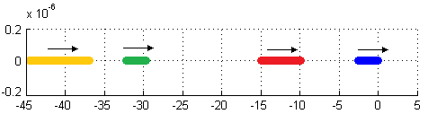
Figure 2: Behaviour of the first four eigenvalues for $\lambda\in[30,40]$.

This should tell us that from this point we have a change in stability properties and also the presence of a new solution branch. Indeed, as we will see, because of the symmetry, there will be at least two new branches for each simple eigenvalue. Going on with the simulations for greater values in the parameter space $\mathcal{D}$ we also observed the crossing of the successive eigenvalues.

Finally, if we solve the eigenvalue problem (31) for the case of $L=2$, we note that a simple eigenvalue of the square plate becomes a multiple eigenvalue with algebraic multiplicity equal to two (see Figure 3). This fact has a relevant consequence from the physical point of view as we will see in the bifurcation diagram later.

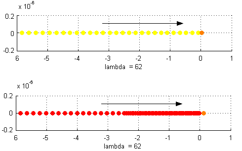
Figure 3: Double eigenvalue for the rectangular plate crossing for $\lambda=62$.

What we just showed is computationally heavy to perform, so to keep in mind the efficiency as key word of the whole analysis, we tried two different ways that validate the result and at the same time reduce the computational time.

Thus we consider the linear problem (11) but in its original form

$$\begin{cases}\Delta^{2}u+\lambda u_{xx}=0\ ,\quad&\text{in}\ \Omega=[0,L]\times[0,1]\\ u=\Delta u=0\ ,\quad&\text{in}\ \partial\Omega\end{cases}$$ (32)

that has non trivial solutions for $m,n=1,2,\dots$ given by

$$u_{m,n}=sin\left(\frac{m\pi x}{L}\right)sin\left(n\pi y\right)\quad\text{if and only if}\quad\lambda_{m,n}=\left(\frac{\pi}{L}\right)^{2}\left[m+\frac{n^{2}L^{2}}{m}\right]^{2},$$ (33)

where $u_{m,n}$ and $\lambda_{m,n}$ can be considered as the eigenfunctions and eigenvalues for this new generalized eigenvalue problem. Now we have a simpler problem, indeed since $\lambda$ is now the eigenvalue, there is no parametrization. This provide us also an explicit expression for the spectra, that we can use to validate the results.

Using the formula (33) we find the exact value for the eigenvalues of the problem (32), that turn out to be the buckling parameter, i.e. the bifurcation point

$$\begin{split}L=1:&\quad\lambda_{1,1}=4\pi^{2},\ \lambda_{2,1}=\frac{25}{4}\pi^{2},\ \lambda_{3,1}=\frac{100}{9}\pi^{2},\ \lambda_{4,1}=\frac{289}{16}\pi^{2},\\ L=2:&\quad\lambda_{2,1}=4\pi^{2},\ \lambda_{3,1}=\frac{169}{36}\pi^{2},\ \lambda_{1,1}=\lambda_{4,1}=\frac{25}{4}\pi^{2},\end{split}$$

indeed we obtain the value $\lambda_{1,1}\simeq 39.47$ predicted in Figure 2 for the square plate, while we note the presence of the double eigenvalue $\lambda_{1,1}=\lambda_{4,1}\simeq 61.68$ that confirms what we saw in Figure 3 for the rectangular one.

Finally, using the techniques in [4, 23], is an easy task to prove the following theorem that provides us a tool to better understand how good is our approximation.

Theorem 4

There exists a strictly positive constant $C$ such that

$$|\lambda-\lambda_{h}|\leq Ch^{2},$$

where $\lambda_{h}$ is an approximation, dependent on the sparsity of the grid, of the true eigenvalue $\lambda$.

The theorem above is crucial when we are dealing with problems for which we do not know an explicit expression of the eigenvalues. For the sake of completeness we provide in Table $1$ and Table $2$ the order of convergence results respectively for the square and rectangular plate, that agree with the theoretical ones.

L=1	h = 1.e-1	h = 6.e-2	h = 1.e-2	h = 6.e-3	Order	Exact
$\lambda_{1,1}$	39.91	39.59	39.48	39.47	1.98	39.47841
$\lambda_{2,1}$	63.70	62.20	61.70	61.69	1.99	61.68502
$\lambda_{3,1}$	116.63	111.54	109.73	109.68	1.97	109.66227

Table 1: Buckling coefficients for the square plate with the average order of convergence

L=2	h = 1.e-1	h = 6.e-2	h = 1.e-2	h = 6.e-3	Order	Exact
$\lambda_{2,1}$	40.74	39.76	39.48	39.48	2.05	39.47841
$\lambda_{3,1}$	49.15	46.97	46.35	46.33	2.34	46.33230
$\lambda_{1,1}$	62.08	61.79	61.68	61.68	1.98	61.68502
$\lambda_{4,1}$	67.44	63.02	61.73	61.69	2.05	61.68502

Table 2: Buckling coefficients for the rectangular plate with the average order of convergence

To conclude this section we briefly discuss also the second straightforward way to reduce the computational complexity of solving multiple times a full order eigenvalue problem. Coming back to the parametrized eigenproblem (31), we can apply again the Reduced Basis method, and thanks to the affine decomposition, we easily obtain in a more efficient way the same behaviour of the results discussed before, as we can see from Figures 4 and 5. We do not discuss further this last approach, in fact we can embed the computation for the eigenproblem (32) in the offline phase.

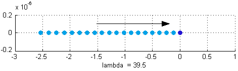
Figure 4: First eigenvalue $\lambda_{1,1}$ in the full order case.

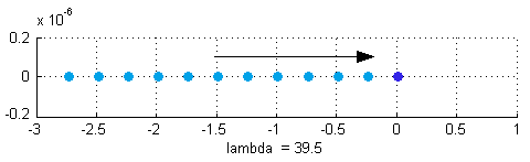
Figure 5: First eigenvalue $\lambda_{1,1}$ in the reduced order case.

4 Results and test problems

In this Section we will show how the buckling phenomena, i.e. the loss of uniqueness of the solution, appears in the equation through the bifurcation diagram, both in the square and rectangular plate cases.

Thus, in order to recap, let us consider the Von Kármán plate equations, with simply supported BCs, in the bi-dimensional domain $\Omega=[0,L]\times[0,1]$ given by

$$\begin{cases}\Delta^{2}u+\lambda u_{xx}=\left[\phi,u\right]\ ,\quad&\text{in}\ \Omega\\ \Delta^{2}\phi=-\left[u,u\right]\ ,\quad&\text{in}\ \Omega\\ u=\Delta u=0\ ,\quad&\text{in}\ \partial\Omega\\ \phi=\Delta\phi=0\ ,\quad&\text{in}\ \partial\Omega\end{cases}$$ (34)

and we are interested in the study of the solution while varying the buckling parameter $\lambda$, which describes the compression along the edges parallel to the $y$-axis.

This model was previously numerically investigated by many authors [10, 13, 33], but as we already said the biggest issue was the computational complexity, that we overcame by means of the Reduced Basis method. We performed all the simulations within FEniCS [3] for the full order case and RBniCS [32] for the reduced order one.

The investigation done with the eigenproblem give us the necessary information that the parameters responsible of the buckling live in the interval $\mathcal{D}=[35,65]$, which we chose as our parameter domain.

4.1 Square plate test case

We present the bifurcation diagram in Figure 6 for the square plate case $\Omega=[0,1]\times[0,1]$. The graph represents for every value of $\lambda\in\mathcal{D}$ on the $x$-axis, the correspondent value of the full order displacement $u$ in its point of maximum modulo. How we predicted previously, we can observe the buckling phenomena from the trivial solution. Moreover, we note that the first bifurcation happens for $\lambda$ value near $\lambda_{1,1}\simeq 39.47$.

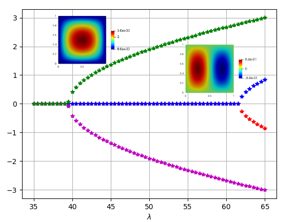
Figure 6: Bifurcation diagram for the square plate.

We did not stop at the first bifurcation, in fact choosing properly the initial guess we have been able to detect also the second bifurcation for the square plate. This result is confirming what we predicted, since for $\lambda$ near $\lambda_{2,1}=61.68$ we obtain other branches.

The physical symmetry issue is evident in both buckling points and the same holds for the rectangular plate. Indeed, once we chose a bifurcation point, a solution from the upper branch is the same solution of the other one, but reflected with respect to the plate plane. Thus, for the first bifurcation near $\lambda_{1,1}$, looking at the contour plot, we observe a one cell like displacement as in Figure 8. While if we look at the second branch, so the one near $\lambda_{2,1}$, we find a two cells like displacement as in Figure 8.

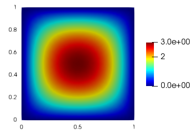
Figure 7: Full order one cell solution for the displacement $u$ with $\lambda=65$ (green branch).

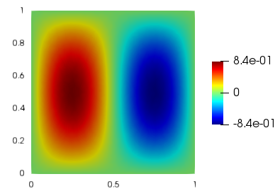
Figure 8: Full order two cells solution for the displacement $u$ with $\lambda=65$ (blue branch).

So for the square plate case we obtained four different solutions for each $\lambda\geq\lambda_{2,1}$.

Moreover, the RB method worked well with this problem. Indeed as we can see in Figure 9, the reduced basis solution approximates perfectly not only the behaviour but also the order of magnitude. The remarkable point is that in order to obtain the solution on the right in Figure 9 we just solved a linear system of dimension $5$ instead of the one given by the Galerkin full order method of order $8\cdot 10^{3}$.

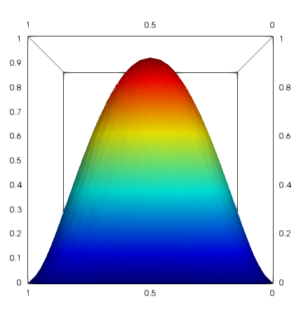
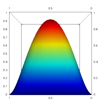
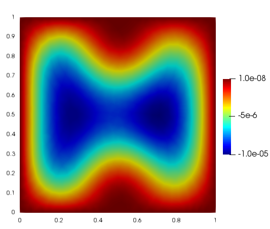
Figure 9: Comparison between the full order solution (on the left) and the reduced order one (on the right) for the displacement $u$ with $\lambda=46$, belonging to the green branch. Below the reduced basis error plot.

We just saw that the Reduced Basis method provides us a useful technique, always based on a full order method (in this case is the Galerkin-Finite Element), that allows us to obtain the same results, at the cost of a small error, but with a huge amount of time saving. To be more precise we present in Table $3$ a convergence results: the error between the truth approximation and the reduced one as a function of $N$. The error reported, $\mathcal{E}_{N}=\max_{\lambda\in\mathcal{D}}{||u_{h}(\lambda)-u_{N}(\lambda)||_{H_{0}^{1}(\Omega)}}$ is the maximum of the approximation error over a uniformly chosen test sample.

We highlight that we present here just the full order bifurcation diagrams since, also in view of Table $3$ and Figure 9, the reduced order one is exactly the same.

$N$	$\cal{E}_{N}$
1	6.61E+00
2	6.90E-01
3	7.81E-02
4	2.53E-02
5	1.88E-02
6	1.24E-02
7	9.02E-03
8	8.46E-03

Table 3: The reduced basis convergence with respect to the number of the basis N for the square plate case.

We remark that we did not implemented the Greedy algorithm here, because a suitable extension of Brezzi-Rappaz-Raviart (BRR) theory for the a posteriori error estimate would be needed [9, 35, 18, 12]. However, applying BRR theory at reduced level is not straightforward and we leave it for further future investigation.

Finally, as regards computational times, a RB evaluation $\lambda\rightarrow u_{N}(\lambda)$ requires just $t_{RB}=100$ ms for $N=8$; while the FE solution $\lambda\rightarrow u_{h}(\lambda)$ requires $t_{FE}=8.17$(s): thus our RB online evaluation is just $1.22\%$ of the FEM computational cost.

4.2 Rectangular plate test case

Now we analyze the case of the rectangular plate, where the domain is $\Omega=[0,2]\times[0,1]$. A huge amount of computations led us to the bifurcation diagram in Figure 10.

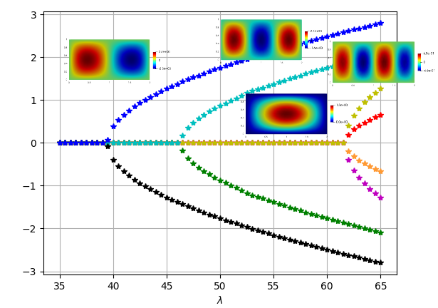
Figure 10: Bifurcation diagram for the rectangular plate.

Now we have a different situation, in fact, varying the length of the domain, we obtained a new bifurcation and also the third one changed its properties. Note that this sensitivity with respect to the dimension of the plate is the main reason why we did not treat also $L$ as a second geometrical parameter along with $\lambda$.

In this case, the solution start branching, as before, from the first ordered eigenvalue $\lambda_{2,1}\simeq 39.47$. Obviously the number of the cells in the contour plot that are formed strictly depends on the length of the domain, for example here the first bifurcation is linked with the two cell configuration as shown in Figure 14.

We observed also a new bifurcation for $\lambda$ value near $46.5$, that is the one with three cells corresponding to the eigenvalue $\lambda_{3,1}\simeq 46.33$, in Figure 14.

Finally, we comment the last, qualitatively different, buckling. As we note in Figure 10, as before, we have a buckling for the $\lambda$ value near to $61.68$ but this time the bifurcation is linked with two eigenvalues. In fact, for the rectangular plate we have a double eigenvalue $\lambda_{1,1}=\lambda_{4,1}$ that is the responsible of this double bifurcation. In practice what we obtained is a point from which start branching two sets of different solutions with one and four cells, respectively in Figure 14 and Figure 14.

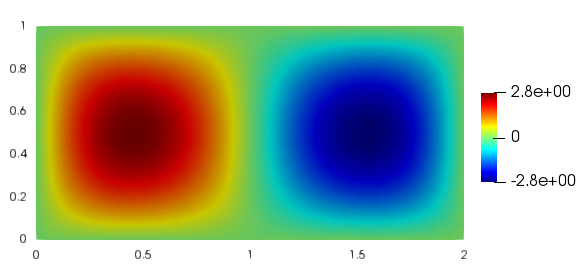
Figure 11: Full order two cells solution for the displacement $u$ with $\lambda=65$ (blue branch).

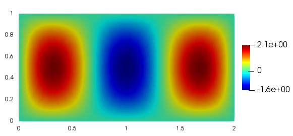
Figure 12: Full order three cells solution for the displacement $u$ with $\lambda=65$ (cyan branch).

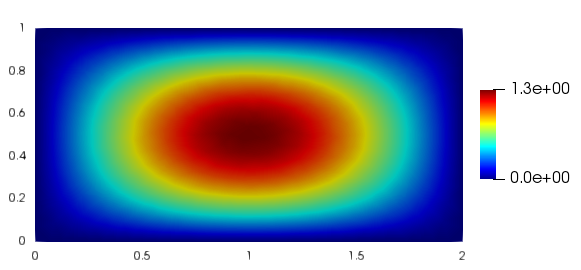
Figure 13: Full order one cell solution for the displacement $u$ with $\lambda=65$ (yellow branch).

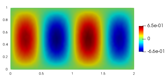
Figure 14: Full order four cells solution for the displacement $u$ with $\lambda=65$ (red branch).

Same conclusions regarding the convergence error $\mathcal{E}_{N}$ and computational savings can be established also in this case. Finally we show that, also for the rectangular plate, the RB method works well approximating efficiently the solution in Figure 15.

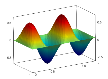
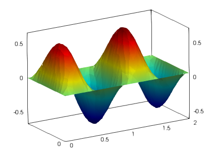
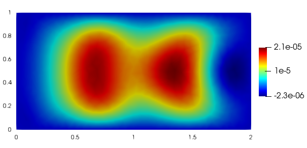
Figure 15: Comparison between the full order solution (on the left) and the reduced order one (on the right) for the displacement $u$ with $\lambda=65$, belonging to the red branch. Below the reduced basis error plot.

4.3 3-D bifurcation test case

In this last numerical result section we want to extend the previous analysis in the case of two parameters, thus obtaining a 3-D bifurcation plot. Considering again the same physical phenomenon, we aim at modelling a compression along the shorter sides of the plate, which is no more uniform on that boundaries. Interested in some practical applications of buckling plates in naval engineering, we parametrized the shape of the compression using a new parameter $\psi$. In fact, the shape of the compression is determined by the function $h$ appearing in (1) thus we can characterize the in-plane compression along $\partial\Omega$ generalizing the corresponding term $\lambda u_{xx}$ in (32) obtaining:

$$\begin{cases}\Delta^{2}u+\lambda\,\text{div}(\sigma\nabla u)=0\ ,\quad&\text{in}\ \Omega\\ u=\Delta u=0\ ,\quad&\text{on}\ \partial\Omega\end{cases}$$ (35)

where $\sigma:\Omega\rightarrow\mathbb{R}^{2\times 2}$, $\sigma\neq 0$ is the plane stress tensor field, which is assumed to satisfy the equilibrium equation:

$$\begin{cases}\sigma^{t}=\sigma\ ,\quad&\text{in}\ \Omega\\ \text{div}\,\sigma=0\ ,\quad&\text{in}\ \Omega\,.\end{cases}$$ (36)

The more general case can be studied, with the uni-axial non-uniform compression given by the stress tensor

$$\sigma(\psi)=\begin{bmatrix}\left(1-\psi\dfrac{y}{L}\right)&0\\ 0&0\end{bmatrix},$$

where $\psi\in[0,2]$ is the parameter that takes care of the linearly varying in-plane load. Moreover, we can recover the standard case analyzed before by choosing $\psi=0$.

Here we want to test the strategy developed in the previous sections in this more complex case, where two parameters are involved in the bifurcation phenomenon. Here we restrict ourself to the most physically relevant behaviour, i.e. the evolution with respect to $\psi$ of the first buckling, for the generalized system

$$\begin{cases}\Delta^{2}u+\lambda\,\text{div}(\sigma(\psi)\nabla u)=\left[\phi,u\right]\ ,\quad&\text{in}\ \Omega\\ \Delta^{2}\phi=-\left[u,u\right]\ ,\quad&\text{in}\ \Omega\\ u=\Delta u=0\ ,\quad&\text{in}\ \partial\Omega\\ \phi=\Delta\phi=0\ ,\quad&\text{in}\ \partial\Omega\ .\end{cases}$$ (37)

Now we can show some preliminary results on the behaviour of the first buckling for the system (37). First of all we can observe in the Figure 17 the 3-D bifurcation plot for the square plate, in which we are describing the first bifurcation point and the post-buckling behaviour, without loss of generality, for each uniformly sampled $\psi\in[0,2]$. For the sake of clearness we show also in Figure 17 the 2-D version of the 3-D plot just presented.

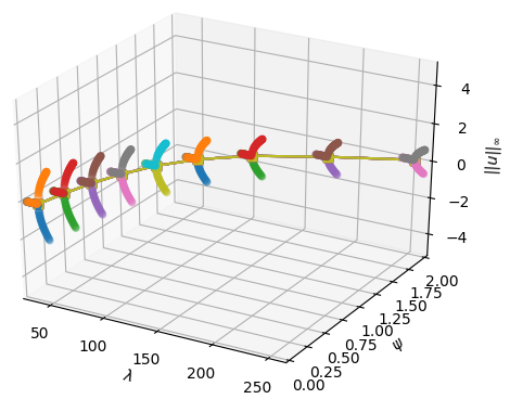
Figure 16: 3-D bifurcation diagram for the square plate.

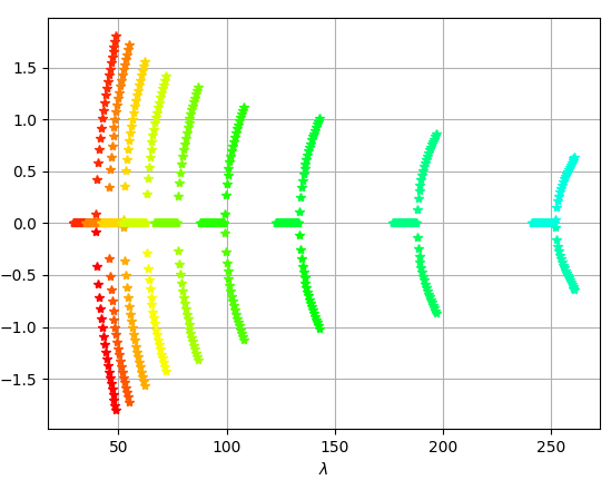
Figure 17: 2-D projected bifurcation diagram for the square plate.

As we can see, the methodology presented in the previous section was able to well detect in the reduced phase the first bifurcation points with respect to the new parameter $\psi$ just introduced. Moreover, we were able to capture correctly the post buckling behaviour, with results validated by the former analysis with $\psi=0$.

Finally we want to remark that here the necessity of the Reduced Order Models is still more evident. In fact, considering only the full order problem, we have to solve a huge linear system (as many times as the following nested iteration): for each Newton step, for each $\lambda$ in the parameter domain, for each (selected) $\psi$ and for each initial guess if one is interested on multiple branches.

5 Future perspectives and developments

In this work we have presented a methodology to properly detect a bifurcation phenomena at different levels, with the support of strong and consolidated theoretical results and the help of computational reduction strategies, allowing to predict efficiently the buckling. We showed the connection of these physical phenomena with the eigenvalue problem, which is fundamental in dealing with different geometry or more complex applications. Several numerical tests were performed confirming the strength of the reduced basis method and its reliability, also in non-linear context. The recovery of eight of the possible solutions shows that, approaching with complex non-linear problems, we need to rely on some backup tool in order to verify that the solution we found is the one we are interested in. Moreover, with this work we showed the consistency of the theoretical results with the numerical ones, but also the necessity to investigate the reduction strategies to apply this methodology on more complex, real applications. The extension of the results for the multi parameter application could be also more relevant since the increasing computational cost.

We plan to extend this work in different directions. The first one is towards the Brezzi-Rappaz-Raviart theory providing the model with an “a posteriori error estimate”. Furthermore, we want to apply this methodology to other kind of problems, such as in fluid structure interaction models, as well as in vibro-acoustics and fluid mechanics frameworks. From the continuum mechanics point of view, we are also interested in the study of different type of plate models, such as the Saint Venant-Kirchhoff, as well as the extension toward the three dimensional Von Kármán equations.

References

- [1] E. Allgower and K. Georg. Introduction to Numerical Continuation Methods. Society for Industrial and Applied Mathematics, 2003.
- [2] A. Ambrosetti and G. Prodi. A Primer of Nonlinear Analysis. Cambridge Studies in Advanced Mathematics. Cambridge University Press, 1995.
- [3] L. Anders, K. Mardal, G. N. Wells, et al. Automated Solution of Differential Equations by the Finite Element Method. Springer, 2012.
- [4] I. Babuška and J. Osborn. Eigenvalue problems. Handbook of numerical analysis, 2:641–787, 1991.
- [5] M. Barrault, N. C. Nguyen, Y. Maday, and A. T. Patera. An “empirical interpolation” method: Application to efficient reduced-basis discretization of partial differential equations. C. R. Acad. Sci. Paris, Série I., 339:667–672, 2004.
- [6] L. Bauer and E. L. Reiss. Nonlinear buckling of rectangular plates. Journal of the Society for Industrial and Applied Mathematics, 13(3):603–626, 1965.
- [7] P. Benner, M. Ohlberger, A. Patera, G. Rozza, and K. Urban, editors. Model Reduction of Parametrized Systems. MS&A Series Vol. 17. Springer International Publishing, 2017.
- [8] M. S. Berger. On Von Kármán’s equations and the buckling of a thin elastic plate, I the clamped plate. Communications on Pure and Applied Mathematics, 20(4):687–719, 1967.
- [9] F. Brezzi, J. Rappaz, and P. A. Raviart. Finite dimensional approximation of nonlinear problems. Numerische Mathematik, 36(1):1–25, 1980.
- [10] Brezzi, F. Finite element approximations of the von k rm n equations. RAIRO. Anal. num r., 12(4):303–312, 1978.
- [11] G. Caloz and J. Rappaz. Numerical analysis for nonlinear and bifurcation problems. Handbook of numerical analysis, 5:487–637, 1997.
- [12] C. Canuto, T. Tonn, and K. Urban. A posteriori error analysis of the reduced basis method for nonaffine parametrized nonlinear pdes. SIAM Journal on Numerical Analysis, 47(3):2001–2022, 2009.
- [13] C. S. Chien and M. S. Chen. Multiple bifurcation in the von Kármán equations. SIAM J. Sci. Comput., 18, 1997.
- [14] P. G. Ciarlet. The Finite Element Method for Elliptic Problems. Classics in Applied Mathematics. Society for Industrial and Applied Mathematics, 2002.
- [15] P. G. Ciarlet. Linear and Nonlinear Functional Analysis with Applications:. Other Titles in Applied Mathematics. Society for Industrial and Applied Mathematics, 2013.
- [16] P. G. Ciarlet and P. A. Raviart. A mixed finite element method for the biharmonic equation. In Proceedings of Symposium on Mathematical Aspects of Finite Elements in PDE, pages 125–145, 1974.
- [17] N. Gräbner, V. Mehrmann, S. Quraishi, C. Schröder, and U. von Wagner. Numerical methods for parametric model reduction in the simulation of disk brake squeal. ZAMM - Journal of Applied Mathematics and Mechanics / Zeitschrift f r Angewandte Mathematik und Mechanik, 96(12):1388–1405, 2016.
- [18] M. A. Grepl, Y. Maday, N. C. Nguyen, and A. T. Patera. Efficient reduced-basis treatment of nonaffine and nonlinear partial differential equations. ESAIM: Mathematical Modelling and Numerical Analysis, 41(3):575–605, 8 2007.
- [19] H. Herrero, Y. Maday, and F. Pla. RB (Reduced Basis) for RB (Rayleigh–Bénard). Computer Methods in Applied Mechanics and Engineering, 261:132–141, 2013.
- [20] J. S. Hesthaven, G. Rozza, and B. Stamm. Certified Reduced Basis Methods for Parametrized Partial Differential Equations. SpringerBriefs in Mathematics. Springer International Publishing, 2015.
- [21] D. B. P. Huynh, A. T. Patera, and G. Rozza. Reduced basis approximation and a posteriori error estimation for affinely parametrized elliptic coercive partial differential equations: Application to transport and continuum mechanics. Archives of Computational Methods in Engineering, 15:229–275, 2008.
- [22] D. B. P. Huynh, F. Pichi, and G. Rozza. Reduced Basis Approximation and A Posteriori Error Estimation: Applications to Elasticity Problems in Several Parametric Settings, pages 203–247. Springer International Publishing, Cham, 2018.
- [23] F. Millar and D. Mora. A finite element method for the buckling problem of simply supported kirchhoff plates. Journal of Computational and Applied Mathematics, 286:68 – 78, 2015.
- [24] A. K. Noor. On making large nonlinear problems small. Comp. Meth. Appl. Mech. Engrg., 34:955–985, 1982.
- [25] A. K. Noor and J. M. Peters. Reduced basis technique for nonlinear analysis of structures. AIAA Journal, 18(4):455–462, April 1980.
- [26] A. K. Noor and J. M. Peters. Multiple-parameter reduced basis technique for bifurcation and post-buckling analysis of composite plates. Int. J. Num. Meth. Engrg., 19:1783–1803, 1983.
- [27] A.T. Patera and G. Rozza. Reduced basis approximation and A posteriori error estimation for Parametrized Partial Differential Equation. MIT Pappalardo Monographs in Mechanical Engineering, Copyright MIT (2007-2010). http://augustine.mit.edu.
- [28] G. Pitton, A. Quaini, and G. Rozza. Computational reduction strategies for the detection of steady bifurcations in incompressible fluid-dynamics: Applications to coanda effect in cardiology. Journal of Computational Physics, 344:534 – 557, 2017.
- [29] G. Pitton and G. Rozza. On the application of reduced basis methods to bifurcation problems in incompressible fluid dynamics. Journal of Scientific Computing, 73(1):157–177, 2017.
- [30] A. Quarteroni. Numerical Models for Differential Problems. MS&A Series Vol. 16. Springer International Publishing, 2017.
- [31] A. Quarteroni, A. Manzoni, and F. Negri. Reduced Basis Methods for Partial Differential Equations: An Introduction. UNITEXT. Springer International Publishing, 2015.
- [32] RBniCS. http://mathlab.sissa.it/rbnics.
- [33] L. Reinhart. On the numerical analysis of the von karman equations: Mixed finite element approximation and continuation techniques. Numerische Mathematik, 39(3):371–404, Oct 1982.
- [34] K. Veroy. Reduced-Basis Methods Applied to Problems in Elasticity: Analysis and Applications. PhD thesis, Massachusetts Institute of Technology, 2003.
- [35] K. Veroy and A. T. Patera. Certified real-time solution of the parametrized steady incompressible navier stokes equations: rigorous reduced-basis a posteriori error bounds. International Journal for Numerical Methods in Fluids, 47(8-9):773–788, 2005.
- [36] T. Von Kármán. Festigkeitsprobleme im maschinenbau. Encyclop die der Mathematischen Wissenschaften, 4, 1910.
- [37] L. Zanon. Model Order Reduction for Nonlinear Elasticity: Applications of the Reduced Basis Method to Geometrical Nonlinearity and Finite Deformation. PhD thesis, RWTH Aachen University, 2017.
- [38] S. Zhang and Z. Zhang. Invalidity of decoupling a biharmonic equation to two poisson equations on non-convex polygons. Int. J. Numer. Anal. Model, 5(1):73–76, 2008.