Asymptotic and scattering behaviour for degenerate multi-solitons in the Hirota equation

Abstract:

We construct all higher order conserved charges from a general two-dimensional zero curvature condition using a Gardner transformation. Employing two of those charges in the definition of a Hamiltonian allows to view the Hirota equations as an integrable $\mathcal{PT}$-symmetric extension of the nonlinear Schrödinger equation. We construct new degenerate multi-soliton solutions from Hirota’s direct method as well as Darboux-Crum transformations based on Jordan states. We study the properties of these solutions, computing their asymptotic time-dependent displacements and also show that their scattering process has a distinct characteristic behaviour different from the nondegenerate counterparts allowing only for interactions of absorb-emit type.

1 Introduction

The Hirota equation [1] is a well known integrable higher order extension of the nonlinear Schrödinger equation (NLSE) [2]. The physical motivation for such an extension was to allow for a more precise description for the wave propagation of pulses in the picosecond regime [3], as the NLSE failed to provide full explanations of some experiments in the high-intensity and short pulse subpicosecond regime [4, 5]. Mathematically this equation is of special interest as it constitutes one of the very few examples for which such type of extensions preserve the integrability. Other known examples of integrable extensions of the NLSE are the NLSE of type I [6], the NLSE of type II [7], the Hirota-modified Korteweg-de Vries equation [8] and the Sasa-Satsuma equation [9].

Here we view the full Hirota equation as $\mathcal{PT}$-symmetrically extended version of NLSE. This simple symmetry property together with the integrability of the system allows for an easy explanation of why the physical quantities associated to the model are real despite the fact that they are computed from complex solutions. We extend here our previous argumentation [10, 11] applied only to the energy of the system to all charges.

Our main focus in this manuscript is the continuation of the study of multi-soliton solutions that have the same speed parameters [12, 13] leading to identical energies of the their one-soliton constituents in their multi-soliton solutions, hence they were referred to as degenerate multi-soliton solutions. Such type of solutions have been found previously for the NLSE in the context of the inverse scattering method [14, 15], where they were referred to as multiple pole solutions. This terminology is somewhat misleading as the poles are not actually in the solutions of the NLSE but in the kernels of the Gel’fand-Levitan-Marchenko equations, that is a specific quantity within the context of the inverse scattering method. In our previous analysis for the Korteweg de-Vries equation [12] and the sine-Gordon equation [13] we showed how to derive these type of solutions in a more transparent way by employing Hirota’s direct method, Darboux-Crum transformations or recursive equations derived from Bäcklund transformations. Here we follow a similar approach for the Hirota equation in the construction of the degenerate multi-soliton solutions.

Our manuscript is organized as follows: In section 2 we employ a Gardner transformation [16] to construct all charges related to a particular two dimensional form of the AKNS-equation. We use two of these charges to construct a Hamiltonian that allows to view the Hirota equations as a $\mathcal{PT}$-symmetrically extended version of NLSE. In section 3 we construct multi-soliton solutions by means of Hirota’s direct method and Darboux-Crum transformation based on Jordan states. In section 4 we study the properties of these solutions. In particular, we compute closed expressions for all higher order charges resulting from concrete multi-solitons solutions, we compute the time-dependent displacements for the one-soliton constituents in the multi-soliton solutions. We also show that unlike as in the degenerate case the scattering process for the degenerate solution only allows for an absorb-emit process. Our conclusions are stated in section 5.

2 The Hirota equation as a $\mathcal{PT}$-symmetrically extended NLSE

We consider here the full Hirota equation [1] in the form

$$\!iq_{t}\!=\!-\alpha\left[q_{xx}+2\left|q\right|^{2}q\right]\!-i\beta\!\left[q_{xxx}+6\left|q\right|^{2}q_{x}\right],$$ (1)

with real constants $\alpha$, $\beta$ and complex valued field $q=q(x,t)$ depending on the position $x$ and time $t$. This equation is known to unify the modified Korteweg-de Vries (mKdV) equation and the NLSE equation, which are obtained from it in the limits $\alpha\rightarrow 0$ and $\beta\rightarrow 0$, respectively. The equation (1) is symmetric with respect to the anti-linear map $\mathcal{PT}:x\rightarrow-x$, $t\rightarrow-t$, $i\rightarrow-i$, $q\rightarrow q$. The term proportional to $\beta$ can be viewed as a $\mathcal{PT}$-symmetric extension of the NLSE. Evidently there exist many such choices and so we briefly explain the origin of the particular form of this extension term that guaranteed the integrability of the model by constructing the Hamiltonian that corresponds to (1) and also all higher order conserved quantities.

We recall that equivalently to the AKNS equation [17], the Hirota equation results as a compatibility equation for the two linear first order differential equations

$$\Psi_{t}=V\Psi\text{\qquad and\qquad\ }\Psi_{x}=U\Psi,$$ (2)

with auxiliary function $\Psi$ and operators $U$, $V$ of the form

$$\Psi=\left(\begin{array}[]{c}\varphi\\ \phi\end{array}\right),\qquad U=\left(\begin{array}[]{cc}-i\lambda&q\\ r&i\lambda\end{array}\right),\qquad V=\left(\begin{array}[]{cc}A&B\\ C&-A\end{array}\right),$$ (3)

with complex valued scalar functions $r$, $q$, $A$, $B$ and $C$. From this starting point the conserved quantities for this system are easily derived from an analogue to the Gardner transform for the KdV field [18, 19, 16, 11]. Defining two new complex valued fields $T(x,t)$ and $\chi(x,t)$ in terms of the components of the auxiliary field $\Psi$ one trivially obtains a local conservation law

$$T:=\frac{\varphi_{x}}{\varphi},\qquad\chi:=-\frac{\varphi_{t}}{\varphi},\quad\Rightarrow~{}~{}~{}T_{t}+\chi_{x}=0.$$ (4)

From the two first rows in the equations (2) we then derive

$$T=q\frac{\phi}{\varphi}-i\lambda\text{,~{}~{}~{}~{}~{}~{}\ \ ~{}}\chi=-A-B\frac{\phi}{\varphi},$$ (5)

so that the local conservation law in (4) is expressed in terms of the as yet unknown quantities $A$, $B$ and $T$

$$T_{t}-\left(A+i\lambda B+\frac{B}{q}T\right)_{x}=0.$$ (6)

The missing function $T$ is then determined by the Ricatti equation

$$T_{x}=i\lambda\frac{q_{x}}{q}+rq-\lambda^{2}+\frac{q_{x}}{q}T-T^{2},$$ (7)

which in turn is obtained by differentiating $T$ in (4) with respect to $x$. The Gardner transformation [18, 19, 16, 11] consists now of expanding $T$ in terms of $\lambda$ and a new field $w$ as $T=-i\lambda[1-w/(2\lambda^{2})]$. This choice is motivated by balancing the first with the fourth and the third and the fifth term when $\lambda\rightarrow\infty$. The factor on the field $w$ is just convenience that renders the following calculations in a simple form. Substituting this expression for $T$ into the Ricatti equation (7) with a further choice $\lambda=i/(2\varepsilon)$, made once more for convenience, yields

$$w+\varepsilon\left(w_{x}-\frac{q_{x}}{q}w\right)+\varepsilon^{2}w^{2}-rq=0.$$ (8)

Up to this point our discussion is entirely generic and the functions $r(x,t)$ and $q(x,t)$ can in principle be any function. Fixing their mutual relation now to $r(x,t)=-q^{\ast}(x,t)$ and expanding the new auxiliary density field as

$$w(x,t)=\mathop{\displaystyle\sum}\limits_{n=0}^{\infty}\varepsilon^{n}w_{n}(x,t),$$ (9)

we can solve (8) for the functions $w_{n}$ in a recursive manner order by order in $\varepsilon$. Iterating these solutions yields

$$w_{n}=\frac{q_{x}}{q}w_{n-1}-(w_{n-1})_{x}-\sum\limits_{k=0}^{n-2}w_{k}w_{n-k-2},\qquad\text{for }n\geq 1.$$ (10)

We compute the first expressions to

$$w_{0} = -\left|q\right|^{2},$$ (11)

$$w_{1} = \frac{1}{2}\left|q\right|_{x}^{2}+\frac{1}{2}\left(qq_{x}^{\ast}-q^{\ast}q_{x}\right),$$ (12)

$$w_{2} = \left|q_{x}\right|^{2}-\left|q\right|^{4}-\frac{1}{2}\left(qq_{x}^{\ast}+q^{\ast}q_{x}\right)_{x}+\frac{1}{2}\left(q^{\ast}q_{xx}-qq_{xx}^{\ast}\right),$$ (13)

$$w_{3} = \left[\frac{5}{4}\left|q\right|^{4}+\frac{1}{2}\left(qq_{xx}^{\ast}+q^{\ast}q_{xx}-\left|q_{x}\right|^{2}\right)\right]_{x}+\frac{1}{2}\left(qq_{xx}^{\ast}-q^{\ast}q_{xx}\right)_{x}$$

$$+\frac{1}{2}\left(3q\left|q\right|^{2}q_{x}^{\ast}-3q^{\ast}\left|q\right|^{2}q_{x}+q_{x}^{\ast}q_{xx}-q_{x}q_{xx}^{\ast}\right).$$

When possible we have also extracted terms that can be written as derivatives, since they become surface terms in the expressions for the conserved quantities, and also those that give a zero contribution to the variation. We note that with regard to the aforementioned $\mathcal{PT}$-symmetry we have $\mathcal{PT}(w_{n})=(-1)^{n}w_{n}$. Since $T$ is a density of a local conservation law, also each function $w_{n}$ can be viewed as a density. We may then define a Hamiltonian density from the two conserved quantities $w_{2}$ and $w_{3}$ as

$$\mathcal{H}(q,q_{x},q_{xx}) \mathcal{=} \mathcal{\alpha}w_{2}+i\beta w_{3}$$ (15)

$$= \mathcal{\alpha}\left(\left|q_{x}\right|^{2}-\left|q\right|^{4}\right)-i\frac{\beta}{2}\left(q_{x}q_{xx}^{\ast}-q_{x}^{\ast}q_{xx}\right)-i\frac{3\beta}{4}\left[\left(q^{\ast}\right)^{2}\left(q^{2}\right)_{x}-q^{2}\left(q^{\ast}\right)_{x}^{2}\right],~{}~{}~{}~{}~{}~{}~{}$$ (16)

with some real constants $\alpha$, $\beta$, where we have dropped all surface terms in (16) and terms with zero variation, such as the last one in (13). We also included an $i$ in front of the $w_{3}$-term to ensure the overall $\mathcal{PT}$-symmetry of $\mathcal{H}$, which prompts us to view the Hirota equation as a $\mathcal{PT}$-symmetric extension of the NLSE. This form will ensure the reality of the total energy of the system, defined by $E(q):=\int\nolimits_{-\infty}^{\infty}$ $\mathcal{H}(q,q_{x},q_{xx})dx$ for a particular solution. It is clear from our analysis that the extension term needs to be of a rather special form as most terms, even when they respect the $\mathcal{PT}$-symmetry, will destroy the integrability of the model, see also [20] for other models.

It is now easy to verify that equation (1) and its conjugate result from varying the Hamiltonian $H=\int$ $\mathcal{H}dx$

$$\!~{}~{}~{}iq_{t}\!=\frac{\delta H}{\delta q^{\ast}}=\sum\nolimits_{n=0}^{\infty}(-1)^{n}\frac{d^{n}}{dx^{n}}\frac{\partial\mathcal{H}}{\partial q_{nx}^{\ast}},~{}~{}\ \ ~{}\!iq_{t}^{\ast}\!=-\frac{\delta H}{\delta q}=\sum\nolimits_{n=0}^{\infty}(-1)^{n}\frac{d^{n}}{dx^{n}}\frac{\partial\mathcal{H}}{\partial q_{nx}},$$ (17)

with Hamiltonian density (16). At this point we also determine the functions

$$A = i\alpha\left|q\right|^{2}-2i\alpha\lambda^{2}+\beta\left(qq_{x}^{\ast}-q^{\ast}q_{x}-4i\lambda^{3}+2i\lambda\left|q\right|^{2}\right),$$ (18)

$$B = i\alpha q_{x}+2\alpha\lambda q+\beta\left(2i\lambda q_{x}-2q\left|q\right|^{2}-q_{xx}+4\lambda^{2}q\right),$$ (19)

$$C = i\alpha q_{x}^{\ast}-2\alpha\lambda q^{\ast}+\beta\left(q_{xx}^{\ast}-2q^{\ast}\left|q\right|^{2}+2i\lambda q_{x}^{\ast}-4\lambda^{2}q^{\ast}\right),$$ (20)

as solutions to the auxiliary equation (2) up to the Hirota equation (1). They serve to compute the function $\chi$ occurring in the local conservation law (6).

3 Construction of degenerate multi-soliton solutions

3.1 Hirota’s direct method

Hirota’s direct method is one of the most transparent and straightforward techniques to find solutions to nonlinear differential equations. We briefly recall the main principle of this method and utilize it to solve Hirota’s equation (1) with a particular focus on how to obtain new degenerate solutions in this context. Factorizing the complex field in (1) as $q(x,t)=g(x,t)/f(x,t)$, with $g(x,t)\in\mathbb{C}$, $f(x,t)\in\mathbb{R}$, it is well known [1] that one can express Hirota’s equation (1) in bilinear form as

$$iD_{t}g\cdot f+\alpha D_{x}^{2}g\cdot f+i\beta D_{x}^{3}g\cdot f = 0,$$ (21)

$$D_{x}^{2}f\cdot f = 2\left|g\right|^{2},$$ (22)

with $D_{x}^{n}$, $D_{t}^{n}$ denoting Hirota derivatives [21] defined by an analogue to the Leibniz rule, albeit with alternating signs,

$$D_{x}^{n}f\cdot g=\sum\limits_{k=0}^{n}\left(\begin{array}[]{l}n\\ k\end{array}\right)(-1)^{k}\frac{\partial^{n-k}}{\partial x^{n-k}}f(x)\frac{\partial^{k}}{\partial x^{k}}g(x).$$ (23)

Exact multi-soliton solutions can be found in a recursive fashion by terminating the formal power series expansions

$$f(x,t)=\mathop{\displaystyle\sum}\limits_{k=0}^{\infty}\varepsilon^{2k}f_{2k}(x,t),\quad\text{and\quad}g(x,t)=\mathop{\displaystyle\sum}\limits_{k=1}^{\infty}\varepsilon^{2k-1}g_{2k-1}(x,t),$$ (24)

at a particular order in $\varepsilon$. The remarkable and well-known feature of this seemingly perturbative approach is that the solutions obtained in this manner are exact for any value of the expansion parameter $\varepsilon$, when the series are suitably terminated.

3.1.1 One-soliton solution

For $\varepsilon=1$ a one-soliton is obtained as

$$q_{1}^{\mu}(x,t)=\frac{g_{1}^{\mu}(x,t)}{1+f_{2}^{\mu}(x,t)},\quad\ \ \text{with~{}\ }g_{1}^{\mu}(x,t)=\tau_{\mu,c}\text{\quad and\quad}f_{2}^{\mu}(x,t)=\frac{\left|\tau_{\mu,c}\right|^{2}}{(\mu+\mu^{\ast})^{2}}.$$ (25)

The building blocks are the functions

$$\tau_{\mu,c}(x,t):=c\tilde{\tau}_{\mu}(x,t),\qquad\tilde{\tau}_{\mu}(x,t):=e^{\mu x+\mu^{2}(i\alpha-\beta\mu)t},$$ (26)

involving the complex constants $c$,$\mu\in\mathbb{C}$. More explicitly, for $c=1$ we have

$$q_{1}^{\mu}(x,t)=\frac{4\delta^{2}e^{x(\delta+i\xi)+it(\delta+i\xi)^{2}(\alpha+i\beta\delta-\beta\xi)}}{4\delta^{2}+e^{2\delta x-2\delta t\left[2\alpha\xi+\beta\left(\delta^{2}-3\xi^{2}\right)\right]}},~{}~{}\ \ \ ~{}\left|q_{1}^{\mu}(x,t)\right|=\frac{4\delta^{2}e^{\delta\left[x-t\left(2\alpha\xi+\beta\left(\delta^{2}-3\xi^{2}\right)\right)\right]}}{4\delta^{2}+e^{2\delta\left[x-t\left(2\alpha\xi+\beta\left(\delta^{2}-3\xi^{2}\right)\right)\right]}}.$$ (27)

with $\mu=\delta+i\xi$, $\delta$,$\xi\in\mathbb{R}$. Defining the real quantities

$$A(x,t) : =x\xi+t\left[\alpha(\delta^{2}-\xi^{2})+\beta\xi(\xi^{2}-3\delta^{2})\right],~{}~{}~{}$$ (28)

$$x_{\pm}^{\delta,\xi} : =t\left[2\alpha\xi+\beta(\delta^{2}-3\xi^{2})\right]\pm\frac{1}{\delta}\ln(2\delta),$$ (29)

we compute the maximum of the modulus for the one-soliton solution to

$$q_{1}^{\mu}(x+x_{+}^{\delta,\xi},t)=\delta\mathop{\mathrm{s}ech}(x\delta)e^{iA(x+x_{+}^{\delta,\xi},t)}~{}~{}~{}\ ~{}~{}\ \ \left|q_{1}^{\mu}(x_{+}^{\delta,\xi},t)\right|=\delta.$$ (30)

Thus while the real and imaginary parts of the one-soliton solution exhibit a breather like behaviour, the modulus is a proper solitary wave with a stable maximum at $\delta$. The solution $q_{1}^{\mu}$ becomes static in the limit to the NLSE $\beta\rightarrow 0$ for real $\mu$, i.e. $\xi=0$, and also in the limit to the mKdV equation $\alpha\rightarrow 0$ when $\delta^{2}=3\xi^{2}$.

3.1.2 Nondegenerate and degenerate two-soliton solution

At the next order in $\varepsilon$ of the expansions (24) we construct a general nondegenerate two-soliton solution as

$$q_{2}^{\mu,\nu}(x,t)=\frac{g_{1}^{\mu,\nu}(x,t)+g_{3}^{\mu,\nu}(x,t)}{1+f_{2}^{\mu,\nu}(x,t)+f_{4}^{\mu,\nu}(x,t)},\quad\ \$$ (31)

with functions

$$g_{1}^{\mu,\nu} = \tau_{\mu,c}+\tau_{\nu,\tilde{c}},$$ (32)

$$g_{3}^{\mu,\nu} = \frac{\left(\mu-\nu\right)^{2}}{\left(\mu+\mu^{\ast}\right)^{2}\left(\nu+\mu^{\ast}\right)^{2}}\tau_{\nu,\tilde{c}}\left|\tau_{\mu,c}\right|^{2}+\frac{\left(\mu-\nu\right)^{2}}{\left(\mu+\nu^{\ast}\right)^{2}\left(\nu+\nu^{\ast}\right)^{2}}\tau_{\mu,c}\left|\tau_{\nu,\tilde{c}}\right|^{2},$$ (33)

$$f_{2}^{\mu,\nu} = \frac{\left|\tau_{\mu,c}\right|^{2}}{\left(\mu+\mu^{\ast}\right)^{2}}+\frac{\tau_{\nu,\delta}\tau_{\mu,c}^{\ast}}{\left(\nu+\mu^{\ast}\right)^{2}}+\frac{\tau_{\mu,c}\tau_{\nu,\tilde{c}}^{\ast}}{\left(\mu+\nu^{\ast}\right)^{2}}+\frac{\left|\tau_{\nu,\tilde{c}}\right|^{2}}{\left(\nu+\nu^{\ast}\right)^{2}},$$ (34)

$$f_{4}^{\mu,\nu} = \frac{\left(\mu-\nu\right)^{2}\left(\mu^{\ast}-\nu^{\ast}\right)^{2}}{\left(\mu+\mu^{\ast}\right)^{2}\left(\nu+\mu^{\ast}\right)^{2}\left(\mu+\nu^{\ast}\right)^{2}\left(\nu+\nu^{\ast}\right)^{2}}\left|\tau_{\mu,c}\right|^{2}\left|\tau_{\nu,\tilde{c}}\right|^{2}.$$ (35)

We have set here also $\varepsilon=1$. As was noted previously in [12, 11, 13] the limit $\mu\rightarrow\nu$ to the degenerate case can not be carried out trivially for generic values of the constants $c$, $\tilde{c}$. However, we find that for the specific choice

$$c=\frac{\left(\mu+\mu^{\ast}\right)\left(\mu+\nu^{\ast}\right)}{\left(\mu-\nu\right)},~{}~{}~{}~{}~{}\tilde{c}=-\frac{\left(\nu+\nu^{\ast}\right)\left(\nu+\mu^{\ast}\right)}{\left(\mu-\nu\right)},$$ (36)

the limit is nonvanishing for all functions in (32)-(35). This choice is not unique, but the form of the denominators is essential to guarantee the limit to be nontrivial. With $c$ and $\tilde{c}$ as in (36) the limit $\mu\rightarrow\nu$ leads to the new degenerate two-soliton solution

$$q_{2}^{\mu,\mu}(x,t)=\frac{\left(\mu+\mu^{\ast}\right)\tilde{\tau}_{\mu}\left[(2+\hat{\tau}_{\mu})+(2-\hat{\tau}_{\mu})\left|\tilde{\tau}_{\mu}\right|^{2}\right]}{1+(2+\left|\hat{\tau}_{\mu}\right|^{2})\left|\tilde{\tau}_{\mu}\right|^{2}+\left|\tilde{\tau}_{\mu}\right|^{4}},$$ (37)

where we introduced the function

$$\hat{\tau}_{\mu}(x,t):=x+\mu t(2i\alpha-3\beta\mu)\left(\mu+\mu^{\ast}\right).$$ (38)

We observe the two different timescales in this solution entering through the functions $\hat{\tau}$ and $\tilde{\tau}$, in a linear and exponential manner, respectively, which is a typical feature of degenerate solutions.

3.2 Darboux-Crum transformations

It is well known that the AKNS equation [17] for many integrable systems can be converted into an eigenvalue equation involving a Hamiltonian of Dirac type. In our case we can read the second equation in (2) as $H\psi=-\lambda\psi$ with $H=-i\sigma_{3}\partial_{x}+V$, $\sigma_{3}$ denoting a standard Pauli matrix, $V_{12}=V_{21}^{\ast}=iq$ and $V_{11}=V_{22}=0$. Taking $H=H_{0}$, Darboux-Crum transformations [22, 23, 24, 25, 26, 27] for Dirac Hamiltonians [28, 29] consist of iterating the equations

$$L_{n}H_{n-1}=H_{n}L_{n}$$ (39)

with the help of some intertwining operators $L_{n}$ that we do not specify here any further. The new Hamiltonians $H_{n}$ satisfy the equations $H_{n}\Psi_{n}=-\mu_{n}\Psi_{n}$. Generalizing also the first equation in (2) by setting $\Psi\rightarrow\Psi_{n}$, the component equations become

$$\begin{array}[]{ll}\left(\varphi_{2j-1}\right)_{x}=\mu_{j}\varphi_{2j-1},&\left(\phi_{2j-1}\right)_{x}=-\mu_{j}\phi_{2j-1},\\ \left(\varphi_{2j-1}\right)_{t}=2\mu_{j}^{2}(i\alpha-2\beta\mu_{j})\varphi_{2j-1},{}{}{}&\left(\phi_{2j-1}\right)_{t}=-2\mu_{j}^{2}(i\alpha-2\beta\mu_{j})\phi_{2j-1},\\ \varphi_{2j}=-\phi_{2j-1}^{\ast},&\phi_{2j}=\varphi_{2j-1}^{\ast},\end{array}~{}~{}~{}\text{for }j=1,\ldots,n,$$ (40)

as explained in more detail in [30]. The solutions to (40)

$$\varphi_{2j-1}=c_{2j-1}e^{\mu_{j}x+2t\mu_{j}^{2}(i\alpha-2\beta\mu_{j})}=\phi_{2j}^{\ast},~{}~{}~{}\phi_{2j-1}=\tilde{c}_{2j-1}e^{-\mu_{j}x-2t\mu_{j}^{2}(i\alpha-2\beta\mu_{j})}=-\varphi_{2j}^{\ast},$$ (41)

are the basic building blocks for the construction of a $n$-soliton solution. They can be expressed in a very compact form as

$$q_{n}=2\frac{\det D_{n}}{\det W_{n}}\,,$$ (42)

with $W_{n}$ and $D_{n}$ denoting $2n\times 2n$-matrices. The matrix $W_{n}$ consists of $n$ columns containing $\varphi_{i}$ and its derivatives $\varphi_{i}^{(n)}:=\partial^{n}\varphi_{i}/\partial x^{n}$ for $i=1,...,2n$ and $n$ columns containing $\phi_{i}$ and its derivatives $\phi_{i}^{(n)}:=\partial^{n}\phi_{i}/\partial x^{n}$

$$W_{n}=\left(\begin{array}[]{cccccccc}\varphi_{1}^{(n-1)}&\varphi_{1}^{(n-2)}&\ldots&\varphi_{1}&\phi_{1}^{(n-1)}&\ldots&\phi_{1}^{\,\prime}&\phi_{1}\\ \varphi_{2}^{(n-1)}&\varphi_{2}^{(n-2)}&\ldots&\varphi_{2}&\phi_{2}^{(n-1)}&\ldots&\phi_{2}^{\,\prime}&\phi_{2}\\ \vdots&\vdots&\ddots&\vdots&\vdots&\ddots&\vdots&\vdots\\ \varphi_{2n}^{(n-1)}&\varphi_{2n}^{(n-2)}&\ldots&\varphi_{2n}&\phi_{2n}^{(n-1)}&\ldots&\phi_{2n}^{\,\prime}&\phi_{2n}\end{array}\right).$$ (43)

The matrix $D_{n}$ is made up of $n-1$ columns containing $\varphi_{i}$ and its derivatives and $n+1$ columns containing $\phi_{i}$ and its derivatives

$$D_{n}=\left(\begin{array}[]{cccccccc}\phi_{1}^{(n-2)}&\phi_{1}^{(n-3)}&\ldots&\phi_{1}&\varphi_{1}^{(n)}&\ldots&\varphi_{1}^{\,\prime}&\varphi_{1}\\ \phi_{2}^{(n-2)}&\phi_{2}^{(n-3)}&\ldots&\phi_{2}&\varphi_{2}^{(n)}&\ldots&\varphi_{2}^{\,\prime}&\varphi_{2}\\ \vdots&\vdots&\ddots&\vdots&\vdots&\ddots&\vdots&\vdots\\ \phi_{2n}^{(n-2)}&\phi_{2n}^{(n-3)}&\ldots&\phi_{2n}&\varphi_{2n}^{(n)}&\ldots&\varphi_{2n}^{\,\prime}&\varphi_{2n}\end{array}\right).$$ (44)

For specific choices of the constants $c_{i}$ and $\tilde{c}_{i}$ involved, the solutions computed from (42) match exactly with the one and two-soliton solutions derived from Hirota’s direct method. Taking for the solutions $q_{1}$ in (42) the constants as $\mu_{1}=(\delta+i\xi)/2$, $c_{1}=\tilde{c}_{1}=-(2\delta)^{-1}$, we obtain (27) and taking $c_{1}=\tilde{c}_{1}=(\mu_{1}-\mu_{2})^{-1}$, $c_{2}=\tilde{c}_{2}=1$ in the solution $q_{2}$ in (42), we get (31) with (36) and the identification $\mu_{1}=\mu$, $\mu_{2}=\nu$.

The degenerate solutions can be obtained in principle by taking the limits $\mu_{1}\rightarrow\mu_{2}\rightarrow\ldots\rightarrow\mu_{n}\rightarrow\mu$, which, however, only leads to nontrivial solutions for very specific choices of the constants $c_{i}$ and $\tilde{c}_{i}$. This is to be expected given the discussion in the precious section. Here we will not specify those constants, but follow a slightly different approach. As pointed out in [30], the nontrivial multi-soliton solutions can be obtained in an alternative and easier fashion in a closed compact form by replacing in (43) and (44) the standard solutions (41) of (40) with Jordan states

$$\varphi_{2j-1} \rightarrow \partial_{\mu}^{j-1}\varphi_{1}\text{,~{}~{}~{}}\phi_{2j-1}\rightarrow\partial_{\mu}^{j-1}\phi_{1}\text{,~{}~{}~{}}$$ (45)

$$\varphi_{2j} \rightarrow \partial_{\mu}^{j-1}\varphi_{2}\text{,~{}~{}~{}}\phi_{2j}\rightarrow\partial_{\mu}^{j-1}\phi_{2}\text{,~{}~{}~{} }$$ (46)

for $j=1,\ldots,n$. These states are essentially solutions to the eigenvalue equation for powers of the Hamitonian operator, see e.g. [12] for more details. Explicitly, the first examples for the matrices $\tilde{D}_{n}$ and $\tilde{W}_{n}$ related to the degenerate solutions are

$$\tilde{D}_{1}=\left(\begin{array}[]{cc}\varphi_{1}^{\prime}&\varphi_{1}\\ \varphi_{2}^{\prime}&\varphi_{2}\end{array}\right),~{}~{}~{}\tilde{W}_{1}=\left(\begin{array}[]{cc}\varphi_{1}&\phi_{1}\\ \varphi_{2}&\phi_{2}\end{array}\right),$$ (47)

$$\tilde{D}_{2}=\left(\begin{array}[]{cccc}\phi_{1}&\varphi_{1}^{\prime\prime}&\varphi_{1}^{\prime}&\varphi_{1}\\ \phi_{2}&\varphi_{2}^{\prime\prime}&\varphi_{2}^{\prime}&\varphi_{2}\\ \phi_{1}^{\prime}&\varphi_{1}^{\prime\prime\prime}&\varphi_{1}^{\prime\prime}&\varphi_{1}^{\prime}\\ \phi_{2}^{\prime}&\varphi_{2}^{\prime\prime\prime}&\varphi_{2}^{\prime\prime}&\varphi_{2}^{\prime}\end{array}\right),~{}~{}~{}\tilde{W}_{2}=\left(\begin{array}[]{cccc}\varphi_{1}^{\prime}&\varphi_{1}&\phi_{1}^{\prime}&\phi_{1}\\ \varphi_{2}^{\prime}&\varphi_{2}&\phi_{2}^{\prime}&\phi_{2}\\ \varphi_{1}^{\prime\prime}&\varphi_{1}^{\prime}&\phi_{1}^{\prime\prime}&\phi_{1}^{\prime}\\ \varphi_{2}^{\prime\prime}&\varphi_{2}^{\prime}&\phi_{2}^{\prime\prime}&\phi_{2}^{\prime}\end{array}\right),$$ (48)

$$\tilde{D}_{3}=\left(\begin{array}[]{cccccc}\phi_{1}^{\prime}&\phi_{1}&\varphi_{1}^{\prime\prime\prime}&\varphi_{1}^{\prime\prime}&\varphi_{1}^{\prime}&\varphi_{1}\\ \phi_{2}^{\prime}&\phi_{2}&\varphi_{2}^{\prime\prime\prime}&\varphi_{2}^{\prime\prime}&\varphi_{2}^{\prime}&\varphi_{2}\\ \phi_{1}^{\prime\prime}&\phi_{1}^{\prime}&\varphi_{1}^{iv}&\varphi_{1}^{\prime\prime\prime}&\varphi_{1}^{\prime\prime}&\varphi_{1}^{\prime}\\ \phi_{2}^{\prime\prime}&\phi_{2}^{\prime}&\varphi_{2}^{iv}&\varphi_{2}^{\prime\prime\prime}&\varphi_{2}^{\prime\prime}&\varphi_{2}^{\prime}\\ \phi_{1}^{\prime\prime\prime}&\phi_{1}^{\prime\prime}&\varphi_{1}^{v}&\varphi_{1}^{iv}&\varphi_{1}^{\prime\prime\prime}&\varphi_{1}^{\prime\prime}\\ \phi_{2}^{\prime\prime\prime}&\phi_{2}^{\prime\prime}&\varphi_{2}^{v}&\varphi_{2}^{iv}&\varphi_{2}^{\prime\prime\prime}&\varphi_{2}^{\prime\prime}\end{array}\right),~{}~{}~{}\tilde{W}_{3}=\left(\begin{array}[]{cccccc}\varphi_{1}^{\prime\prime}&\varphi_{1}^{\prime}&\varphi_{1}&\phi_{1}^{\prime\prime}&\phi_{1}^{\prime}&\phi_{1}\\ \varphi_{2}^{\prime\prime}&\varphi_{2}^{\prime}&\varphi_{2}&\phi_{2}^{\prime\prime}&\phi_{2}^{\prime}&\phi_{2}\\ \varphi_{1}^{\prime\prime\prime}&\varphi_{1}^{\prime\prime}&\varphi_{1}^{\prime}&\phi_{1}^{\prime\prime\prime}&\phi_{1}^{\prime\prime}&\phi_{1}^{\prime}\\ \varphi_{2}^{\prime\prime\prime}&\varphi_{2}^{\prime\prime}&\varphi_{2}^{\prime}&\phi_{2}^{\prime\prime\prime}&\phi_{2}^{\prime\prime}&\phi_{2}^{\prime}\\ \varphi_{1}^{iv}&\varphi_{1}^{\prime\prime\prime}&\varphi_{1}^{\prime\prime}&\phi_{1}^{iv}&\phi_{1}^{\prime\prime\prime}&\phi_{1}^{\prime\prime}\\ \varphi_{2}^{iv}&\varphi_{2}^{\prime\prime\prime}&\varphi_{2}^{\prime\prime}&\phi_{2}^{iv}&\phi_{2}^{\prime\prime\prime}&\phi_{2}^{\prime\prime}\end{array}\right),$$ (49)

with $\varphi_{1}=ce^{\mu x+2t\mu^{2}(i\alpha-2\beta\mu)}=\phi_{2}^{\ast}$, $\phi_{1}=\tilde{c}_{1}e^{-\mu x-2t\mu^{2}(i\alpha-2\beta\mu)}=-\varphi_{2}^{\ast}$. The degenerate $n$-soliton solutions are then computed as

$$q_{n}^{n\mu}(x,t)=2\frac{\det\tilde{D}_{n}}{\det\tilde{W}_{n}},$$ (50)

with only one spectral parameter $\mu$ left.

4 Properties of degenerate multi-soliton solutions

4.1 Real charges from complex solutions

Let us now verify that all the charges resulting from the densities in (10) are real. Defining the charges as the integrals of the charge densities

$$Q_{n}=\mathop{\displaystyle\int}\nolimits_{-\infty}^{\infty}w_{n}dx$$ (51)

we expect from the $\mathcal{PT}$-symmetry behaviour $\mathcal{PT}(w_{n})=(-1)^{n}w_{n}$ that $Q_{2n}\in\mathbb{R}$ and $Q_{2n+1}\in i\mathbb{R}$. Taking now $q_{1}$ to be in the form (30) and shifting $x\rightarrow x+x^{+}$ in (51), we find from (10) that the only contribution to the integral comes from the iteration of the first term, that is

$$Q_{n}=\mathop{\displaystyle\int}\nolimits_{-\infty}^{\infty}\left(\frac{q_{x}}{q}\right)^{n}w_{0}dx.$$ (52)

It is clear that the second term in (10), $(w_{n-1})_{x}$, does not contribute to the integral as it is a surface term. Less obvious is the cancellation of the remaining terms, which can however be verified easily. For the one-soliton solution (30) the charges (52) become

$$Q_{n} = -\delta^{2}\mathop{\displaystyle\int}\nolimits_{-\infty}^{\infty}\left[i\xi-\delta\tanh(x\delta)\right]^{n}\mathop{\mathrm{s}ech}^{2}(x\delta)dx$$ (53)

$$= -\left|\delta\right|\mathop{\displaystyle\int}\nolimits_{-1}^{1}\left(i\xi-\delta u\right)^{n}du$$ (54)

$$= -\left|\delta\right|\mathop{\displaystyle\sum}\nolimits_{k=0}^{n}\frac{n!}{(k+1)!(n-k)!}\delta^{k}(i\xi)^{n-k}\left[1+(-1)^{k}\right].$$ (55)

Since only the terms with even $k$ contribute to the sum in (55), it is evident from this expression that $Q_{2n}\in\mathbb{R}$ and $Q_{2n+1}\in i\mathbb{R}$.

Of special interest is the energy of the system resulting from the Hamiltonian (15). For the one-soliton solution (30) we obtain

$$E(q_{1}^{\mu})=\mathcal{\alpha}Q_{2}+i\beta Q_{3}=2\left|\delta\right|\left[\alpha\left(\xi^{2}-\frac{\delta^{2}}{3}\right)+\beta\xi\left(\delta^{2}-\xi^{2}\right)\right].$$ (56)

As expected, due to the $\mathcal{PT}$-symmetry the energy is real despite being computed from a complex field.

The energy of the two-soliton solution (37) is computed to

$$E(q_{2}^{\mu,\mu})=2E(q_{1}^{\mu}).$$ (57)

The doubling of the energy for the degenerate solution in (37) when compared to the one-soliton solution is of course what we expect from the fact that the model is integrable and the computation constitutes therefore an indirect consistency check. We expect (57) to generalize to $E(q_{3}^{n\mu})=nE(q_{1}^{\mu})\,$, which we verified numerically for $n=3$ using the solution (50).

4.2 Asymptotic behaviour

Next we compute the asymptotic displacement in the scattering process in a similar fashion as discussed in more detail in [12, 11, 13]. The analysis relies on computing the asymptotic limits of the multi-soliton solutions and comparing the results with the tracked one-soliton solution. As a distinct point we track the maxima of the one-soliton solution (25) within the two-soliton solution. Similarly as the one-soliton, the real and imaginary parts of the two-soliton solution depend on the function $A(x,t)$, as defined in (28), occurring in the argument of the $\sin$ and $\cos$ functions. This makes it is impossible to track a distinct point with constant amplitude. However, as different values for $A$ only produce an internal oscillation we can fix $A$ to any constant value without affecting the overall speed.

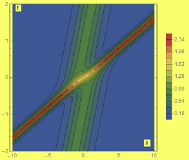
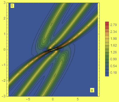
We start with the calculation for the degenerate two-soliton solution and illustrate the above behaviour in figure 1 for a concrete choice of $A$.

Figure 1: Real part of the degenerate two-soliton solution (37) for the Hirota equations (1) at small values of times for $\alpha=1$, $\beta=2$, $\delta=3/2$, $\xi=1$ with generic $A(x,t)$ in the left panel and fixed $A=\pi/3$ in the right panel.

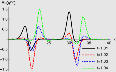
The functions with constant values of $A$ can be seen as enveloping functions similar to those employed for the computation of displacements in breather functions, see e.g. [13]. Thus with $A(x,t)=A$ taken to be constant we calculate the four limits

$$\lim_{t\rightarrow\pm\infty}\!q_{2}^{\mu,\mu}(x_{+}^{\delta,\xi}+\Delta(t),t) = \pm\frac{\beta\delta^{2}\cos A-\delta(\alpha-3\beta\xi)\sin A}{\sqrt{\beta^{2}\delta^{2}+(\alpha-3\beta\xi)^{2}}}\pm i\frac{\delta(\alpha-3\beta\xi)\cos A+\beta\delta^{2}\sin A}{\sqrt{\beta^{2}\delta^{2}+(\alpha-3\beta\xi)^{2}}}$$

$$\lim_{t\rightarrow\pm\infty}\!q_{2}^{\mu,\mu}(x_{-}^{\delta,\xi}-\Delta(t),t) = \mp\frac{\beta\delta^{2}\cos A+\delta(\alpha-3\beta\xi)\sin A}{\sqrt{\beta^{2}\delta^{2}+(\alpha-3\beta\xi)^{2}}}\pm i\frac{\delta(\alpha-3\beta\xi)\cos A-\beta\delta^{2}\sin A}{\sqrt{\beta^{2}\delta^{2}+(\alpha-3\beta\xi)^{2}}}$$

with time-dependent displacement

$$\Delta(t)=\frac{1}{\delta}\ln\left[2\delta\left|t\right|\sqrt{\beta^{2}\delta^{2}+(\alpha-3\beta\xi)^{2}}\right].$$ (58)

Using the limits form above we obtain the same asymptotic value in all four cases for the displaced modulus of the two-soliton solution

$$\lim_{t\rightarrow\pm\infty}\left|q_{2}^{\mu,\mu}(x_{\pm}^{\delta,\xi}\pm\Delta(t),t)\right|=\delta.$$ (59)

In the limit to the NLSE, i.e. $\beta\rightarrow 0$, our expression for $\Delta(t)$ agrees precisely with the result obtained in [14].

We have here two options to interpret these calculations: As the compound two-soliton structure is entirely identical in the two limits $t\rightarrow\pm\infty$ and its individual one-soliton constituents are indistinguishable we may conclude that there is no overall displacement for the individual one-soliton constituents. Alternatively we may assume that the two one-soliton constituents have exchanged their position and thus the overall time-dependent displacement is $2/\delta\ln(2\delta)+2\Delta(t)$.

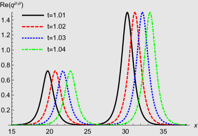
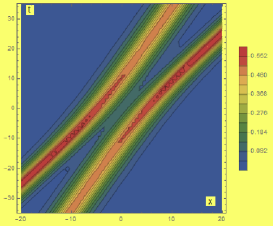
For comparison we compute next the displacement for the nondegenerate two-soliton solution (31) with $c=\tilde{c}=1$ and parameterization $\mu=\delta+i\xi$, $\nu=\rho+i\sigma$ where $\delta$,$\xi$,$\rho$,$\sigma\in\mathbb{R}$. For definiteness we take $x_{+}^{\delta,\xi}>x_{+}^{\rho,\sigma}$ and calculate the asymptotic limits

$$\lim_{t\rightarrow+\infty}\left|q_{2}^{\mu,\nu}(x_{+}^{\delta,\xi}+\frac{1}{\delta}\tilde{\Delta},t)\right| = \lim_{t\rightarrow-\infty}\left|q_{2}^{\mu,\nu}(x_{+}^{\delta,\xi},t)\right|=\delta,$$ (60)

$$\lim_{t\rightarrow+\infty}\left|q_{2}^{\mu,\nu}(x_{+}^{\rho,\sigma},t)\right| = \lim_{t\rightarrow-\infty}\left|q_{2}^{\mu,\nu}(x_{+}^{\delta,\xi}+\frac{1}{\rho}\tilde{\Delta},t)\right|=\rho,$$ (61)

with constant

$$\tilde{\Delta}=\ln\left[\frac{(\delta+\rho)^{2}+(\xi-\sigma)^{2}}{(\delta-\rho)^{2}+(\xi-\sigma)^{2}}\right].$$ (62)

Thus, while the faster one-soliton constituent with amplitude $\delta$ is advanced by the amount $\tilde{\Delta}/\delta$, the slower one-soliton constituent with amplitude $\rho$ is regressed by the amount $\tilde{\Delta}/\rho$. We compare the two-soliton solution with the two one-soliton solutions in figure 2.

Figure 2: Nondegenerate two-soliton solution compared to two one-soliton solutions for large values of $|t|$ for $\alpha=1.1$, $\beta=0.9$, $\delta=0.8$, $\xi=0.4$, $\rho=0.5$, $\sigma=0.6$ in the left panel. Degenerate two-soliton solution compared to two one-soliton solutions for large values of $|t|$ for $\alpha=1.5$, $\beta=2.3$, $\delta=0.25$, $\xi=0.6$ in the right panel.

We also observe that while the time-dependent displacement $\Delta(t)$ in (58) for the degenerate solution depends explicitly on the parameters $\alpha$ and $\beta$, the constant $\tilde{\Delta}$ in (62) is the same for all values of $\alpha$ and $\beta$. In particular it is the same in the Hirota equation, the NLSE and the mKdV equation. The values for $\alpha$ and $\beta$ only enter through $x_{+}^{\rho,\sigma}$ in the tracking process.

4.3 Scattering behaviour

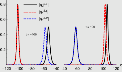
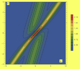
Besides having a distinct asymptotic behaviour, the degenerate multi-solitons also display very particular features during the actual scattering event near $x=t=0$ when compared to the nondegenerate solutions. For the nondegenerate two-soliton solution three distinct types of scattering processes at the origin have been identified. Using the terminology of [8] they are merge-split denoting the process of two solitons merging into one soliton and subsequently separating while each one-soliton maintains the direction and momentum of its trajectory, bounce-exchange referring to two-solitons bouncing off each other while exchanging their momenta and absorb-emit characterizing the process of one soliton absorbing the other at its front tail and emitting it at its back tail, see figure 3.

Figure 3: Different types of nondegenerate two-soliton scattering processes for the solution (31). Left panel: merge-split scattering with $\alpha=1.1$, $\beta=0.9$, $\rho=2.5$, $\xi=0.4$, $\delta=-0.8$, $\sigma=0.6$. Middle panel: bounce-exchange scattering with $\alpha=1.1$, $\beta=0.9$, $\rho=-0.6$, $\xi=0.1$, $\delta=0.5$, $\sigma=0.2$. Right panel: absorb-emit scattering with $\alpha=1.1$, $\beta=0.9$, $\rho=-1.5$, $\xi=0.4$, $\delta=-0.8$, $\sigma=0.6$.

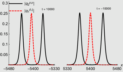
For the degenerate multi-soliton solutions the merge-split and bounce-exchange scattering is not possible and only the absorb-emit scattering process occurs as seen in figure 4.

Figure 4: Absorb-emit scattering processes for degenerate two-solitons (37) with $\alpha=1.1$, $\beta=0.9$, $\delta=0.8$, $\xi=0.1$ (left panel) and three-solitons (50) with $\alpha=1.1$, $\beta=0.9$, $\delta=0.8$, $\xi=0.4$ (right panel).

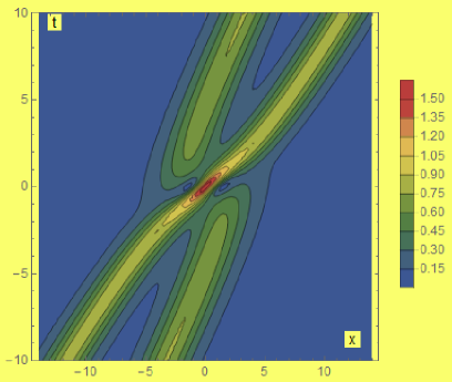
This feature is easy to understand when considering the behaviour of the solution at $x=t=0$. As was argued in [8] the different behaviour can classified by their behaviour as being either convex downward or concave upward at $x=t=0$ together with occurrence of additional local maxima. For the degenerate two-soliton solution we find $\left.\partial\left|q_{2}^{\mu,\mu}(x,t)\right|/\partial x\right|_{x=0,t=0}=0$ and $\left.\partial^{2}\left|q_{2}^{\mu,\mu}(x,t)\right|/\partial x^{2}\right|_{x=0,t=0}=-10\left|\delta\right|^{3}$, which means this solution is always concave at $x=t=0$. In addition, we find that $\mathop{\mathrm{R}e}\left.q_{2}^{\mu,\mu}(x,t)\right|_{x=0,t=0}$ and $\mathop{\mathrm{I}m}\left.q_{2}^{\mu,\mu}(x,t)\right|_{x=0,t=0}$ are always concave and convex at $x=t=0$, respectively. Hence, we always have the emergence of additional local maxima, such that the behaviour must be of the absorb-emit type. In figure 4 we display this scattering behaviour for the degenerate two and three-soliton solutions in which the distinct features of the absorb-emit behaviour are clearly identifiable.

We observe that the dependence on the parameters $\alpha~{}$and $\beta$ of the degenerate and nondegenerate solution is now reversed when compared to the asymptotic analysis. While the type of scattering in the nondegenerate case is highly sensitive with regard to $\alpha~{}$and $\beta$, it is entirely independent of these parameters in the degenerate case.

5 Conclusions

We constructed all charges resulting from the AKNS equation (2) and (3) by means of a Gardner transformation. Two of the charges were used to define a Hamiltonian whose functional variation led to the Hirota equation. The behaviour of these charges under $\mathcal{PT}$-symmetry suggests to view the Hirota system as an integrable extended version of NLSE. This point of view allows for an easy generalization of previous arguments [10, 11] that guarantee the reality of the energy to all higher order charges. We computed a closed analytic expression for all charges involving a particular one-soliton solution.

Explicit multi-soliton solutions from Hirota’s direct method as well as the Darboux-Crum transformations were derived and we showed how to construct degenerate solutions in both schemes. As observed previously, the application of Hirota’s direct method relies on choosing the arbitrary constants in the solutions in a very particular way. When using Darboux-Crum transformations the degenerate solutions are obtained by replacing standard solutions in the underlying auxiliary eigenvalue problem by Jordan states.

From the asymptotic behaviour of the degenerate two-soliton solution we computed the new expression for the time-dependent displacement. As the degenerate one-soliton constituents in the multi-soliton solutions are asymptotically indistinguishable one can not decide whether the two one-solitons have actually exchanged their position and therefore the time-dependent displacement can be interpreted as an advance or delay or whether the two one-solitons have only approached each other and then separated again. The analysis of the actual scattering event allows for both views. It would be very interesting to investigate the statistical behaviour of a degenerate soliton gas along the lines of, for instance [31, 32, 33, 34], which should certainly exhibit different characteristics as the underlying statistical distributions would be based on indistinguishable rather than distinguishable particles.

We showed that degenerate two-solitons may only scatter via an absorb-emit process, that is by one soliton absorbing the other at its front tail and subsequently emitting it at the back tail. Since the model is integrable all multi-particle/soliton scattering processes may be understood as consecutive two particle/soliton scattering events, so that the two-soliton scattering behaviour extends to the multi-soliton scattering as we demonstrated.

Acknowledgments: JC is supported by a City, University of London Research Fellowship and would like to thank Vincent Caudrelier, Alexander Mikhailov and Simon Ruijsenaars for discussions and references on the NLSE. We would also like to thank Francisco Correa for discussions.

References

- [1] R. Hirota, Exact envelope-soliton solutions of a nonlinear wave equation, J. Math. Phys. 14(7), 805–809 (1973).
- [2] A. Shabat and V. Zakharov, Exact theory of two-dimensional self-focusing and one-dimensional self-modulation of waves in nonlinear media, Sov. Phys. JETP 34(1), 62–69 (1972).
- [3] L. F. Mollenauer, R. H. Stolen, and J. P. Gordon, Experimental observation of picosecond pulse narrowing and solitons in optical fibers, Phys. Rev. Lett. 45(13), 1095 (1980).
- [4] F. M. Mitschke and L. F. Mollenauer, Discovery of the soliton self-frequency shift, Optics Letters 11(10), 659–661 (1986).
- [5] J. P. Gordon, Theory of the soliton self-frequency shift, Optics letters 11(10), 662–664 (1986).
- [6] D. Anderson and M. Lisak, Nonlinear asymmetric self-phase modulation and self-steepening of pulses in long optical waveguides, Phys. Rev. A 27(3), 1393 (1983).
- [7] H. Chen, Y. Lee, and C. Liu, Integrability of nonlinear Hamiltonian systems by inverse scattering method, Physica Scripta 20(3-4), 490 (1979).
- [8] S. Anco, N. T. Ngatat, and M. Willoughby, Interaction properties of complex modified Korteweg–de Vries (mKdV) solitons, Physica D: Nonlinear Phenomena 240(17), 1378–1394 (2011).
- [9] N. Sasa and J. Satsuma, New-type of soliton solutions for a higher-order nonlinear Schrödinger equation, J. Phys. Soc. Japan 60(2), 409–417 (1991).
- [10] J. Cen and A. Fring, Complex solitons with real energies, J. Phys. A: Math. Theor. 49(36), 365202 (2016).
- [11] J. Cen, F. Correa, and A. Fring, Time-delay and reality conditions for complex solitons, J. of Math. Phys. 58(3), 032901 (2017).
- [12] F. Correa and A. Fring, Regularized degenerate multi-solitons, Journal of High Energy Physics 2016(9), 8 (2016).
- [13] J. Cen, F. Correa, and A. Fring, Degenerate multi-solitons in the sine-Gordon equation, J. Phys. A: Math. Theor. 50, 435201 (2017).
- [14] E. Olmedilla, Multiple pole solutions of the non-linear Schrödinger equation, Physica D: Nonlinear Phenomena 25(1-3), 330–346 (1987).
- [15] C. Schiebold, Asymptotics for the multiple pole solutions of the nonlinear Schrödinger equation, Nonlinearity 30(7), 2930 (2017).
- [16] B. A. Kupershmidt, On the nature of the Gardner transformation, Journal of Mathematical Physics 22(3), 449–451 (1981).
- [17] M. J. Ablowitz, D. J. Kaup, A. C. Newell, and H. Segur, Nonlinear-evolution equations of physical significance, Phys. Rev. Lett. 31(2), 125 (1973).
- [18] R. M. Miura, C. S. Gardner, and M. D. Kruskal, Korteweg-de Vries equation and generalizations. II. Existence of conservation laws and constants of motion, Journal of Mathematical physics 9(8), 1204–1209 (1968).
- [19] R. M. Miura, The Korteweg-de Vries Equation: A Survey of Results, SIAM Review 18, 412–459 (1976).
- [20] A. Fring, PT-symmetric deformations of integrable models, Phil. Trans. Royal Soc. London A: Math., Phys. and Eng. Sci. 371(1989), 20120046 (2013).
- [21] R. Hirota, The direct method in soliton theory, volume 155, Cambridge University Press, 2004.
- [22] G. Darboux, On a proposition relative to linear equations, physics/9908003, Comptes Rendus Acad. Sci. Paris 94, 1456–59 (1882).
- [23] M. M. Crum, Associated Sturm-Liouville systems, The Quarterly Journal of Mathematics 6(1), 121–127 (1955).
- [24] V. B. Matveev and M. A. Salle, Darboux transformation and solitons, (Springer, Berlin) (1991).
- [25] F. Correa and M. S. Plyushchay, Hidden supersymmetry in quantum bosonic systems, Annals of Physics 322(10), 2493–2500 (2007).
- [26] F. Correa, V. Jakubskỳ, L.-M. Nieto, and M. S. Plyushchay, Self-isospectrality, special supersymmetry, and their effect on the band structure, Phys. Rev. Lett. 101(3), 030403 (2008).
- [27] J. Mateos-Guilarte and M. S. Plyushchay, Perfectly invisible PT-symmetric zero-gap systems, conformal field theoretical kinks, and exotic nonlinear supersymmetry, arXiv1710.00356 (2017).
- [28] L. M. Nieto, A. A. Pecheritsin, and B. F. Samsonov, Intertwining technique for the one-dimensional stationary Dirac equation, Annals. of Phys. 305(2), 151–189 (2003).
- [29] F. Correa and V. Jakubskỳ, Confluent Crum-Darboux transformations in Dirac Hamiltonians with PT-symmetric Bragg gratings, Phys. Rev. A 95(3), 033807 (2017).
- [30] J. Cen, F. Correa, and A. Fring, Integrable nonlocal Hirota equations, arXiv:1710.11560 (2017).
- [31] N. Gupta and B. Sutherland, Investigation of a class of one-dimensional nonlinear fields, Phys. Rev. A 14(5), 1790 (1976).
- [32] F. Mertens and H. Büttner, The soliton-gas analogy for the Toda lattice, Phys. Lett. A 84(6), 335–337 (1981).
- [33] K. Sasaki, Soliton-breather approach to classical sine-Gordon thermodynamics, Phys. Rev. B 33(4), 2214 (1986).
- [34] E. G. Shurgalina and E. N. Pelinovsky, Nonlinear dynamics of a soliton gas: Modified Korteweg–de Vries equation framework, Phys. Lett. A 380(24), 2049–2053 (2016).